Crop-Masked Vegetation Indices and TerraClimate for District-Level Wheat Yield Prediction in Kazakhstan: SAVI Advantage, Climate Dominance, and Temporal Transferability Limits

Abstract

Accurate district-level wheat yield forecasting is critical for Kazakhstan, the world’s seventh-largest wheat exporter. Prior remote-sensing studies typically compute vegetation indices over entire administrative units without isolating cropland, diluting the crop-specific signal and biassing remote-sensing–climate comparisons. A 25-year (2000–2024) dataset was assembled for 149 Kazakh districts (n = 2378 district–year observations, ~390 features), integrating crop-masked Sentinel-2/Landsat-7 optical indices, Sentinel-1 SAR, TerraClimate, and station, soil, and terrain data, and a HistGradientBoosting model was evaluated under both spatial (GroupKFold) and temporal (expanding-window) cross-validation. Ten-metre cropland masking substantially improved index–yield correlations, especially early in the season, and SAVI consistently outperformed NDVI from June onward. The best configuration—crop-masked optical indices with TerraClimate—achieved R² = 0.646 (RMSE = 0.349 t/ha) under spatial cross-validation, whereas adding SAR yielded no significant gain. Pre-season winter-climate data (January–March) reached about 91% of full-year accuracy, enabling forecasts months before sowing. Critically, temporal cross-validation produced a markedly lower mean R² = 0.413, a predictability gap (ΔR² = 0.233) that provides a more representative estimate of operational forecast accuracy. Residuals showed no significant spatial autocorrelation. These results indicate that cropland masking and joint reporting of spatial and temporal cross-validation are valuable for yield prediction in semi-arid continental environments.

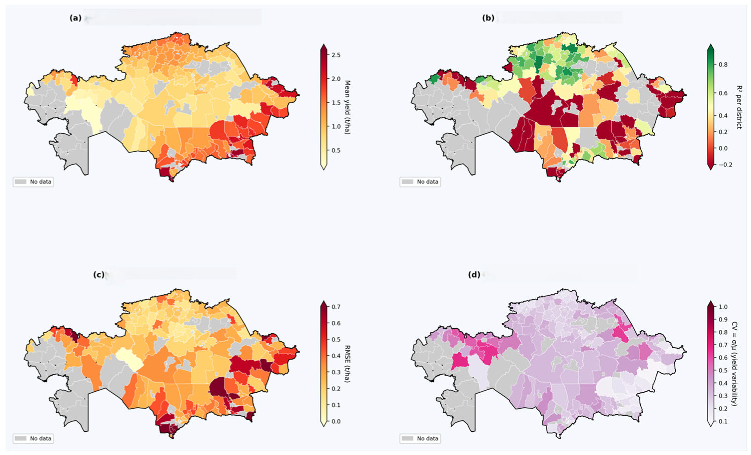
1. Introduction

Wheat (Triticum aestivum L.) provides approximately 20% of global caloric intake and remains the primary dietary staple across the developing world [1]. Global production faces a dual structural threat: rising demand driven by population growth projected to reach 9.7 billion by 2050 [2] and declining yield stability under accelerating climate change. The IPCC Sixth Assessment Report projects global average wheat yields to decline by 2–6% per decade under moderate warming and by up to 13% under high-emissions pathways by mid-century. Central Asia faces disproportionate reductions of 10–25%, driven by increasing drought frequency, heat stress during grain filling, and shifts in precipitation seasonality [3]. Against this backdrop, sub-national yield forecasting systems are an operational necessity for food security planning and trade management, not merely a research aspiration.

Kazakhstan occupies a singular strategic position in global food systems as the world’s seventh-largest wheat exporter and the primary cereal supplier for five landlocked Central Asian republics whose collective import dependency exceeds 60% of domestic consumption [4,5]. 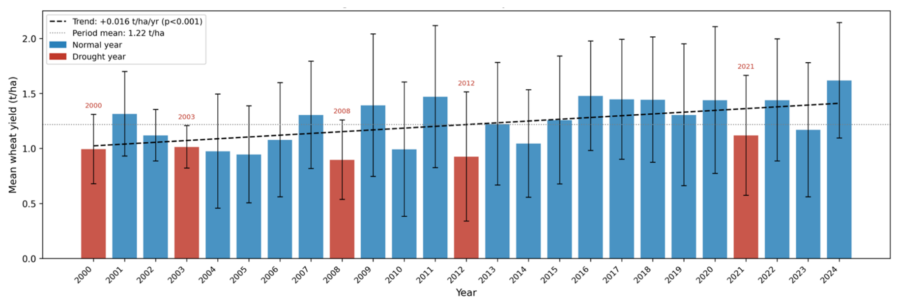The country’s 12+ million harvested wheat hectares operate under extreme continental conditions—annual precipitation of 250–450 mm concentrated in spring and early summer, inter-annual coefficients of variation exceeding 35%, and yield swings routinely surpassing 50% between consecutive seasons [6]. The 2021 drought, the most spatially extensive since independence, reduced the official (harvested-area-weighted) national mean yield to 0.98 t/ha and triggered emergency import protocols in Kyrgyzstan, Tajikistan, and Uzbekistan [7]. These dynamics expose a systemic gap: the Bureau of National Statistics and Ministry of Agriculture require district-level preliminary forecasts by June—two to three months before the August–September harvest—yet no validated early-warning model exists at this spatial resolution [8].

Optical remote-sensing (RS) yield forecasting rests on Monteith’s [9] light-use efficiency framework, which links time-integrated absorbed photosynthetically active radiation—proxied by NDVI [10]—to harvestable biomass. The field has since shifted from single-index regression to multi-source machine learning (ML) frameworks integrating satellite time series, gridded climate data, and ancillary layers [11]. Gradient boosting models on Sentinel-2 or MODIS imagery achieve R² = 0.60–0.85 for dryland wheat [12], with June–July identified as the most predictive window [13,14]. Such ensembles (LightGBM, XGBoost, HistGradientBoosting) consistently outperform linear models and deep learning on moderate-sized heterogeneous tabular data [15,16,17], and HistGradientBoostingRegressor (HistGBM; scikit-learn v1.8.0) additionally handles missing values natively [18].

A persistent limitation in the yield prediction literature is the computation of vegetation indices as district-wide spatial averages without isolating cropland pixels. Sentinel-2 (10 m) outperforms coarser sensors in mixed-landscape districts by reducing sub-pixel land-cover confusion [19,20], yet even at 10 m, district-mean indices remain dominated by non-crop surfaces where agricultural intensity is low. In Kazakhstan’s bright-soil, low-LAI wheat belt, high calcareous soil reflectance additionally contaminates NDVI through soil background [21]. The Soil-Adjusted Vegetation Index (SAVI; Huete [21]) applies an L-factor correction to suppress this contamination and has shown advantages over NDVI for wheat in temperate and semi-arid systems [22,23], with further support from dryland comparisons where soil brightness is a primary spectral confounder [24]. However, SAVI has not been evaluated for Kazakhstan’s dryland spring wheat at a district scale. Sentinel-1 C-band SAR provides complementary all-weather observations: VH cross-polarised backscatter tracks canopy volume scattering from crop stems and leaves through the season [25,26], capturing structural information unavailable to optical sensors under cloud. SAR–optical integration has improved wheat accuracy in European systems [27,28], yet Sentinel-1-based yield prediction for Central Asia remains absent from the peer-reviewed literature.

For multi-source comparisons, gridded climate datasets—notably TerraClimate [29]—consistently explain a larger fraction of yield variance than unmasked vegetation indices in rainfed dryland systems [30,31], a relationship theoretically grounded in Kazakhstan’s direct precipitation–yield coupling [31,32] but statistically compounded by the absence of cropland masking in RS workflows [33]. A critical, underappreciated methodological issue is cross-validation (CV) design. Standard spatial k-fold CV—the dominant evaluation protocol in published yield prediction studies [15,34]—inflates apparent accuracy relative to expanding-window evaluation that preserves the temporal ordering of the data because spatially separate folds share inter-annual climate signals between training and test sets [34]. This inflation is pronounced in systems with strong temporal autocorrelation, such as Kazakhstan’s drought-prone continental wheat belt.

Despite Kazakhstan’s pivotal role in global cereal markets, it remains severely underrepresented in the peer-reviewed literature. Bokusheva et al. [35] pioneered AVHRR-based Vegetation and Temperature Condition Indices (VCI, TCI) at national scale. Kussul et al. [20] developed deep-learning land cover and crop type classification for Ukrainian agricultural regions, demonstrating how sub-pixel mixing at coarse resolution systematically confounds crop-specific spectral signals in continental steppe landscapes—an analytical challenge directly relevant to Kazakhstan. Sadenova et al. [36] applied ML and neural-network methods to multiple crops at experimental-farm level in East Kazakhstan (R² = 0.60–0.81), but without cropland masking, temporal validation, or SAR. A structured search retrieved only two qualifying peer-reviewed studies [35,36], confirming that Kazakhstan remains critically understudied relative to regions where Sentinel-2-based wheat yield frameworks are already established (for example, Central Asia [37] and North America [38]). This gap is consequential given Kazakhstan’s combination of extreme continentality, bright calcareous soils, and a dryland spring wheat phenology that differs fundamentally from all well-studied systems.

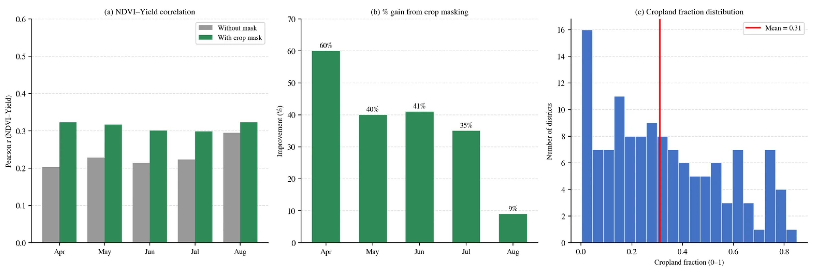
Building on this review, five methodological gaps remain. First, most sub-national studies compute vegetation indices across whole administrative units without isolating cropland pixels [11]. In Kazakhstan, where the mean district cropland fraction is only ~35% (IQR ≈ 10–57%), this masking effect has never been quantified with 10 m land-cover products. Second, many ML yield studies include previous-year yield as a predictor [15,24], which encodes persistent spatial productivity differences, limits operational utility, and precludes comparison with observation-only models. Third, spatial k-fold CV dominates the literature [34] yet inflates apparent accuracy relative to temporally out-of-sample evaluation, and no Kazakhstan study has reported temporal CV as its primary metric. Fourth, although SAVI advantages are theoretically predicted [39] and documented in analogous bright-soil systems [22,23,24], SAVI has never been evaluated at a district scale in Kazakhstan with multi-decadal, multi-source data. Fifth, Central Asia is severely underrepresented: only two qualifying sub-national studies exist for Kazakhstan [35,36], making methodological transfer from better-studied systems unreliable without empirical validation.

This study addresses all five gaps through the following specific research questions:

RQ1: How does 10 m cropland masking using Google Dynamic World and ESA WorldCover affect the predictive power of optical RS indices, SAR data, and the relative performance hierarchy of these data sources versus gridded climate data?

RQ2: Which data source combination provides the strongest wheat yield signal without any lagged features, and does adding SAR to optical–climate combinations genuinely improve prediction?

RQ3: Does SAVI demonstrate measurable empirical advantages over NDVI for Kazakhstan’s semi-arid wheat belt, both in univariate correlations and in multi-source ML feature importance?

RQ4: How early in the growing season can reliable yield forecasts be issued, and what is the temporal transferability of statistical models to unseen future years including unprecedented drought conditions?

RQ5: What are the top predictors of Kazakhstan wheat yield without lagged features, and how does predictability vary across agroclimatic zones?

2. Materials and Methods

2.1. Study Area and Agroclimatic Zonation

The study encompasses 149 administrative districts (rayons) across all 16 oblasts of Kazakhstan (40–55° N, 46–87° E), covering approximately 2.72 million km² (Figure 1). Kazakhstan’s wheat system is highly regionalised, reflecting the country’s pronounced north–south climatic gradient from subhumid continental steppe to hyper-arid desert. Five primary agroclimatic zones are defined for analysis (Figure 1), delimited by climatic and agronomic criteria following the national zonation of the Ministry of Agriculture of Kazakhstan:

•

North Grain Belt (Akmola, Kostanay, North Kazakhstan regions; 42 districts; mean elevation 240 m; annual precipitation 300–400 mm; cropland fraction 0.52): The national wheat heartland, accounting for ~70% of national wheat area. Entirely rainfed spring wheat (sowing: late April–May; harvest: August–September).

•

East Zone (Abay, East Kazakhstan, Pavlodar; 27 districts; mean elevation 425 m; annual precipitation 280–380 mm; cropland fraction 0.32): Transitional zone with higher elevation and topographic complexity; mixed rainfed and supplemental irrigation systems.

•

South Irrigated Zone (Turkistan, Jambyl, Jetisu, Almaty, Kyzylorda; 44 districts; mean elevation 728 m; annual precipitation 250–400 mm; cropland fraction 0.26): Semi-arid to arid with significant irrigated wheat area, predominantly winter wheat varieties. Highest absolute mean yield (1.61 t/ha) but lowest RS predictability due to unobservable irrigation management.

•

West Arid zone (Aktobe, Atyrau, West Kazakhstan; 18 districts; mean elevation 165 m; annual precipitation 150–250 mm; cropland fraction 0.26): Driest agricultural zone; very low and highly variable yields (mean 0.43 t/ha, CV = 1.23); marginal croplands with high year-to-year area fluctuations. Mangystau oblast is shown in Figure 1a for geographic completeness but is excluded from all yield analyses due to the absence of district-level wheat production statistics.

•

Central Zone (Karaganda, Ulytau; 8 districts: Abay, Bukhar-Zhyrau, Karkaraly, Nura, Osakarov, and Shet in Karaganda Region; Jezkazgan and Ulytau District in Ulytau Region): Transitional steppe; limited wheat cultivation; included in the national model but analysed separately with caution due to small sample size (n = 188 district–year observations). Zhanaarka District was excluded due to fewer than five non-zero yield records [40,41].

2.2. Wheat Yield Data

Official district-level wheat yield statistics (t/ha) for 2000–2024 were obtained from the Bureau of National Statistics of the Republic of Kazakhstan (stat.gov.kz) [8]. Yield data represent harvested production divided by harvested area as reported by agricultural enterprises and farms at the rayon (district) level. After quality control—excluding records with implausible values (yield > 6.0 t/ha or <0.05 t/ha, representing <0.3% of observations)—the complete dataset comprises N = 2878 district–year records. Of these, 2378 records have non-zero wheat yield and constitute the modelling subset (n = 2378). The remaining 500 records correspond to district–year combinations where wheat was not cultivated or yield data were not reported; these are retained for data completeness statistics but excluded from all predictive experiments. No imputation was applied; districts with missing yield records in a given year were excluded from the corresponding model configuration.

The national yield distribution is right-skewed (skewness = 0.41): mean = 1.11 t/ha, SD = 0.67 t/ha, median = 1.07 t/ha, range [0.01, 3.86] t/ha. Six years recorded national mean wheat yields below 1.0 t/ha (2000, 2004, 2005, 2008, 2010, 2012), representing 24% of the 25-year study period, each associated with hydrothermal coefficient (HTC; Selyaninov, 1937 [42]) values below 1.0 during the critical June–July grain-filling window [43]. The temporal trend estimated by ordinary least squares amounts to +0.018 t/ha yr⁻¹ (p < 0.001; R² = 0.38), reflecting technology adoption and improved cultivar deployment, but does not reduce inter-annual variability [8,44].

2.3. Remote Sensing Data

2.3.1. Optical Vegetation Indices

Monthly composite optical vegetation indices were extracted from Sentinel-2 Level-2A surface reflectance imagery (10 m; 2016–2024) and Landsat-7 ETM+ surface reflectance (30 m; 2000–2015), both processed within Google Earth Engine (GEE) (Google LLC, Mountain View, CA, USA). Monthly composites were constructed as pixel-wise median values after cloud and cloud-shadow masking using QA60 bitmask flags for Sentinel-2 and the CFMask algorithm for Landsat-7 [45]. Four spectral indices were computed at native pixel resolution before spatial aggregation:

The Normalised Difference Vegetation Index (NDVI), introduced by Rouse et al. [46] and further developed by Tucker [10], is a chlorophyll-sensitive spectral index widely used as a proxy for photosynthetic activity and fraction of absorbed photosynthetically active radiation (fAPAR):

$$NDVI={\displaystyle \frac{NIR-Red}{NIR+Red}}$$

(1)

where NIR and Red are the surface reflectances in the near-infrared and red bands, respectively. The Soil-Adjusted Vegetation Index (SAVI), proposed by Huete [21] to suppress soil-brightness contamination in low-LAI canopies, is defined as follows:

$$SAVI=\left[{\displaystyle \frac{NIR-Red}{NIR+Red+L}}\right]\times \left(1+L\right)$$

(2)

where L = 0.5 is the empirically determined soil-adjustment factor recommended by Huete [21] for intermediate vegetation cover densities (LAI 1.5–3.0), characteristic of Kazakhstan’s spring wheat fields at peak canopy. The Enhanced Vegetation Index (EVI), developed by Huete et al. [47] to additionally correct for aerosol and atmospheric effects:

$$EVI=G\times {\displaystyle \frac{(NIR-Red)}{(NIR+C_1\times Red-C_2\times Blue+L)}}$$

(3)

with coefficients $G$ = 2.5, $C_{1 }$ = 6, $C_2$= 7.5, $L$ = 1.0 (standard MODIS EVI coefficients [47]). EVI values outside the physically plausible range [−0.3, 0.9]—the established physical bound for EVI over vegetated and bare-soil surfaces, beyond which values are non-physical by construction—were excluded (~2.3% of pixels) as numerical artefacts arising over bright calcareous soil backgrounds where the denominator approaches zero [47]. The Normalised Difference Water Index (NDWI), introduced by Gao [48] as a proxy for canopy water content:

$$NDWI={\displaystyle \frac{NIR-SWIR}{NIR+SWIR}}$$

(4)

Pixel-level index values were spatially aggregated to district-level means exclusively within cropland-masked pixels, yielding 12 monthly features per index (4 indices × 12 months = 48 optical features per district–year). For the Landsat-7 SLC-off period (2003–2015), monthly temporal compositing effectively compensates for ~22% pixel loss per scene: mean valid-pixel fraction within crop-masked districts during April–September was 88.9% for the SLC-off period versus 88.7% for the Sentinel-2 era, indicating negligible systematic bias in data completeness. This completeness check does not, however, address radiometric and spectral differences between the 30 m Landsat-7 ETM+ and 10 m Sentinel-2 MSI sensors; the resulting cross-sensor offset and the way the modelling framework accommodates it are examined explicitly in Section 4 (Uncertainty and cross-sensor consistency).

2.3.2. SAR Data (Sentinel-1)

Sentinel-1 C-band SAR Ground Range Detected (GRD) images in Interferometric Wide (IW) swath mode were processed in GEE (2016–2024; spatial resolution 10 m, resampled to 1 km after masking). Monthly median composites of four backscatter features were extracted within cropland masks: VH backscatter (${\sigma }_{VH}^0$, dB), VV backscatter (${\sigma }_{VV}^0$, dB), polarisation ratio (${\sigma }_{VH}^0/{\sigma }_{VV}^0$), and the Radar Vegetation Index (RVI) [49,50]:

$$RVI=4{\sigma }_{VH}^0/{(\sigma }_{VV}^0+{\sigma }_{VH}^0)$$

(5)

RVI approaches unity for randomly oriented vegetation volume scatterers and approaches zero for bare soil, making it sensitive to canopy structural development throughout the growing season [51]. The physical basis for SAR–crop relationships in C-band (5.6 cm wavelength) rests on the sensitivity of VH (cross-polarised) backscatter to random volume scattering from crop stems and leaves, while VV (co-polarised) backscatter responds to both canopy volume and soil surface roughness [25]. SAR data are unavailable for 2000–2015, resulting in structurally missing values for 68% of the full-period dataset—handled natively by the HistGradientBoosting missing-value mechanism. Total: 24 SAR features per district–year.

2.4. Cropland Masking

A central methodological contribution of this study is the systematic application of 10 m resolution cropland masks to all spectral index and SAR backscatter computations prior to spatial aggregation to district level. Without masking, district-mean vegetation indices are diluted by non-crop land covers (steppe grassland, shrubland, bare soil, urban structures), which typically occupy 48–74% of Kazakhstan’s administrative districts by area. Two complementary land cover products were used depending on the data availability period:

•

Google Dynamic World v1 (Google LLC, Mountain View, CA, USA) (GDW; 2016–2024) [52]: a 10 m per-pixel near-real-time land use/land cover product derived from Sentinel-2 using a fully convolutional neural network architecture, providing continuous class probability scores $p_{crops}$ ∈ [0, 1] for ten land cover classes. The annual cropland mask $M_{GDW}$ is defined as follows:

$$M_{GDW(x,y,t)}=\left\{\begin{array}{c}1, if p_{crops}(x,y,t)\ge \theta \\ 0, otherwise\end{array}\right.$$

(6)

where $\theta =0.3$. The threshold θ = 0.3 was selected following sensitivity analysis over $\theta$ ∈ {0.2, 0.3, 0.4, 0.5}, balancing commission and omission errors. Brown et al. [51] report an overall accuracy of 72.8% and a crop-class of F1 = 0.72.

•

ESA WorldCover 2021 (European Space Agency, Paris, France) (WC2021; applied retrospectively to 2000–2015) [52]: a 10 m global static land cover map with 11 classes derived from combined Sentinel-1 and Sentinel-2 imagery, with overall accuracy 74.4% and cropland F1 = 0.77 [52]. Applied as a temporally fixed mask for the Landsat era; residual uncertainty from land-use change between 2000 and 2021 is acceptable given the documented stability of Kazakhstan’s agricultural boundaries since approximately 2005.

The masked district-level mean index value for district d at time t is computed as follows [33]:

$$\overline{I}\left(d,m\right)={\displaystyle \frac{{\sum }_{(x,y)\in {\Omega }_d}M(x,y,t)\times I(x,y,t)}{{\sum }_{(x,y)\in {\Omega }_d}M(x,y,t)}}$$

(7)

where $I(x,y,t)$ is the pixel-level spectral index, $M\left(x,y,t\right)ϵ\left\{\mathrm{0,1}\right\}$ is the binary cropland mask, and ${\Omega }_4$ denotes the spatial domain of district d. The district cropland fraction is retained as an additional predictor:

$$f_{areal}\left(d,t\right)={\displaystyle \frac{{\sum }_{(x,y)\in {\Omega }_d}M(x,y,t)}{\left|{\Omega }_d\right|}}$$

(8)

2.5. Hyperparameter Selection and Justification

HistGradientBoostingRegressor hyperparameters were fixed a priori: max_depth = 5, learning_rate = 0.08, min_samples_leaf = 15, l2_regularization = 1.0, random_state = 42, based on published recommendations for medium-sized heterogeneous tabular datasets [18,53]. Robustness was assessed across five alternative configurations spanning max_depth ∈ {3, 5, 8} and learning_rate ∈ {0.03, 0.08, 0.15} (Table S2). Hyperparameters were deliberately fixed a priori rather than tuned per fold. With only three spatial groups and five temporal test years, an inner tuning loop would have little data to select over and, more importantly, optimising hyperparameters on the same data used for evaluation tends to produce optimistically biassed performance estimates. Fixing a single, literature-recommended configuration across all experiments keeps the seven ablation models strictly comparable and isolates the effect of the data sources rather than of model tuning. The five-configuration grid above therefore functions as a sensitivity analysis, confirming that the source ranking is insensitive to the specific hyperparameter values, in lieu of a nested cross-validation that the small number of folds does not support. Because the shapefile-based KMeans fold assignment was unavailable for these supplementary runs, region-based fold assignment was used as a fallback; consequently, absolute R² values in the sensitivity analysis (M5 range: 0.545–0.563) are lower than in the main analysis, which uses centroid-based folds. Despite this difference in fold construction, M5 (optical + TerraClimate) achieves the highest R² in all five configurations, consistently outperforming both single-source baselines M1 (optical) and M3 (TerraClimate). The conclusion that multi-source fusion outperforms any single source is therefore robust to hyperparameter variation.

2.6. EVI Exclusion Rationale

Although EVI is included in the feature set and its correlation with yield reported (Table 6, it is excluded from the primary modelling features due to known incompatibility of MODIS-derived atmospheric correction coefficients (C₁ = 6.0, C₂ = 7.5) with Sentinel-2 spectral band configurations. These coefficients were optimised for MODIS sensor characteristics and do not transfer directly to Sentinel-2, producing unreliable values over the bright calcareous soils common in Kazakhstan’s arid zones. Diagnostic evaluation confirmed this instability: the peak EVI–yield Pearson correlation did not exceed |r| ≈ 0.05 in any growing-season month—an order of magnitude weaker than NDVI or SAVI. In addition, a substantial fraction of district–month EVI values fell outside the physically plausible range [−0.3, 0.9], with extreme outliers spanning several orders of magnitude where the denominator approaches zero (Table 6). Future implementations should adopt the two-band EVI2 formulation [54], which uses sensor-agnostic coefficients and has been validated for Sentinel-2 applications in semi-arid environments.

2.7. Climate and Ancillary Data

TerraClimate [29] provided nine gridded monthly climate variables at ~4 km spatial resolution for 2000–2024 (108 features; 100% temporal completeness): maximum and minimum temperature (T_max, T_min, °C), total precipitation (P, mm), Palmer Drought Severity Index (PDSI), potential evapotranspiration (PET, mm), soil moisture content (SM, mm), snow water equivalent (SWE, mm), downwelling solar radiation (Rad, W m⁻²), and wind direction (WD). Abatzoglou et al. [29] validated TerraClimate against independent station observations, reporting median Pearson correlations of r = 0.92–0.98 for temperature variables and r = 0.72–0.85 for precipitation at monthly resolution globally.

Meteorological station records (125 features; 62.4% temporal completeness) include daily air temperature, soil temperature at 5 and 10 cm depth, relative humidity, vapour pressure deficit (VPD), wind speed, total precipitation, snow depth, and atmospheric pressure from the national station network. Station observations were interpolated to district centroids using inverse distance weighting (IDW) from the three nearest stations, following Shepard [55]:

$$\widehat{z}={\displaystyle \frac{{\sum }_i{w}_i{z}_i}{{\sum }_i{w}_i}}, w_i={\displaystyle \frac{1}{d_i^2}}$$

(9)

where $z_i$ is the observed meteorological value at station i, d_i is the Euclidean distance from district centroid to station i, and the power parameter p = 2 is standard for meteorological interpolation [55].

Hydrological station discharge data (32 features; 60.4% completeness) comprise monthly mean river discharge and water level from the national network, aggregated to catchment-averaged values for districts intersecting major river systems (Irtysh, Ishim, Tobol, Ural, Syr Darya).

Soil and terrain attributes (4 static features; 100% completeness) include elevation from SRTM 90 m DEM and clay content (%), sand content (%), and soil organic carbon (SOC, g kg⁻¹) from SoilGrids 250 m [56]. A complete summary of all data sources is provided in

Table 1. Summary of input data sources for the multi-source wheat yield prediction framework. Completeness refers to the fraction of district–year observations with non-missing values. N Features = number of monthly features per district–year.

Source	Product/Variable	Period	Resolution	N Features	Completeness	Masking	Reference
Optical RS	NDVI, EVI, SAVI, NDWI	2000–2024	10 m (S2)/30 m (L7)	48	99.8%	Yes (DW/WC)	[51,52]
SAR	VH/VV ratio, RVI	2016–2024	10 m (S1)	24	99.1%	Yes	[50,57]
TerraClimate	T_max, T_min, P, PDSI, PET, SM, SWE, Rad, WD × 12	2000–2024	~4 km	108	100%	No	[29]
Meteorological data	T_air, T_soil, RH, VPD, Wind, P, Snow, P_atm (IDW)	2000–2024	Station	125	62.4%	No	[58]
Hydrology data	River discharge, water level × 12 months + seasonal	2000–2024	Catchment	32	60.4%	No	–
Soil/Terrain	Elevation (SRTM), Clay%, Sand%, SOC (SoilGrids)	Static	90–250 m	4	100%	No	[56]
Engineered	NDVI anomalies, precip anomalies, GDD, seasonal aggregates, year	–	–	46	99.8%	–	–

Abbreviations: NDVI, Normalised Difference Vegetation Index; SAVI, Soil-Adjusted Vegetation Index; EVI, Enhanced Vegetation Index; NDWI, Normalised Difference Water Index; VH/VV, SAR polarisation channels; RVI, Radar Vegetation Index; P, precipitation; T, temperature; VPD, vapour pressure deficit; PDSI, Palmer Drought Severity Index; PET, potential evapotranspiration; SM, soil moisture; SWE, snow water equivalent; Rad, solar radiation; WD, wind direction; SOC, soil organic carbon; GDD, growing degree days; IDW, inverse distance weighting.

.

2.8. Feature Engineering

Forty-five analytically engineered features were derived from primary data sources (NDVI anomalies: 13; precipitation anomalies: 13; growing degree days: 13; seasonal aggregates: 6), plus one structural covariate (calendar year; 1 feature) included to capture the documented long-term yield trend (+0.018 t/ha·yr⁻¹), totalling 46 features (Table 1). All lagged yield variables were explicitly excluded to ensure operational forecasting validity (i.e., the model cannot access the yield value from the previous year when issuing a forecast).

NDVI anomalies (13 features): Monthly deviation from the 25-year district-specific climatological mean, following the anomaly based approach of Becker-Reshef et al. [13]

$$∆NDVI\left(d,m,t\right)=NDVI\left(d,m,t\right)-\overline{NDVI}(d,m)$$

(10)

where $\overline{NDVI}\left(d,m\right)=1/T{\sum }_{t=1}^{T}NDVI(d,m,t)$ is the long-term mean for district d in calendar month m over T = 25 years. Twelve monthly anomalies plus the April–August mean anomaly are included.

Precipitation anomalies (13 features): Standardised monthly deviation, a primary predictor of yield variance in Kazakhstan’s rainfed wheat system [30,31]:

$$∆P^{*}\left(d,m,t\right)={\displaystyle \frac{P\left(d,m,t\right)-\overline{P}(d,m)}{{\sigma }_p(d,m)}}$$

(11)

where $\overline{P}\left(d,m\right)$ and ${\sigma }_p\left(d,m\right)$ are the long-term mean and standard deviation of precipitation for district $d$ and month $m$. Twelve monthly anomalies plus the March–May cumulative precipitation anomaly are included.

Growing degree days (13 features): Monthly accumulated thermal time for spring wheat development, computed using a base temperature $T_{base}$ = 0 °C, following McMaster and Wilhelm [59]:

$$GDD\left(d,m,t\right)=\mathrm{m}\mathrm{a}\mathrm{x}({\overline{T}}_{air}\left(d,m,t\right)-T_{base},0)\times n_m$$

(12)

where ${\overline{T}}_{air}\left(d,m,t\right)$ is the mean daily air temperature in month $m$, $n_m$ is the number of days in the month, and $T_{base}$ = 0 °C is the standard base temperature for spring wheat (Triticum aestivum L.) [59]. Twelve monthly $GDD$ values plus the April–August seasonal total are included.

Seasonal aggregates (6 features): spring precipitation total P_spring = ΣP(Mar–May); seasonal aridity index AI = ΣPET(Apr–Aug)/ΣP(Apr–Aug), following UNESCO [43]; maximum winter snow water equivalent max(SWE, Jan–Apr); late frost index (number of days with T_min < 0 °C after 15 April); winter mean temperature mean(T_air, Nov–Mar); and summer vapour pressure deficit mean(VPD, Jun–Aug).

2.9. Machine Learning Framework

2.9.1. Model Selection and Architecture

HistGradientBoostingRegressor (HistGBM; scikit-learn v1.8.0), the scikit-learn implementation of histogram-based gradient boosting functionally equivalent to LightGBM [18], was selected as the primary prediction algorithm based on three criteria: (1) native handling of missing values through histogram bin assignment, essential given the 37.6% and 68% missing rates in meteorological and SAR features, respectively; (2) demonstrated superiority over Random Forest on heterogeneous tabular datasets of moderate size [15,17]; and (3) computational efficiency for the 2878 × ~400 feature design matrix.

The gradient boosting algorithm sequentially fits K additive regression trees by minimising the regularised empirical risk [32]:

$$\mathcal{L}\left(\widehat{Y}\right)={\sum }_{i=1}^n\mathcal{l}\left(y_i,{\widehat{y}}_i\right)+{\sum }_{k=1}^K\Omega \left(f_k\right)$$

(13)

where $\mathcal{l}\left(y_i,{\widehat{y}}_i\right)=1/2{(y_i-{\widehat{y}}_i)}^2$ is the squared-error loss for observation i, $f_k$ is the k-th regression tree, and $\Omega \left(f_k\right)=\mathsf{\lambda }{‖w‖}^2$ is the L2 leaf-weight regularisation term [18]. Each tree f_k is fitted to the negative gradient (pseudo-residuals) of the loss with respect to the current ensemble prediction. Hyperparameters were fixed a priori based on published recommendations [16,17] and held constant across all experiments to prevent fold-specific overfitting: max_iter = 150, max_depth = 5, learning rate = 0.08, min samples leaf = 15, L2_regularization = 1.0, random state = 42.

2.9.2. Cross-Validation Strategies

Two structurally distinct cross-validation strategies were implemented, following the framework of Roberts et al. [34], to quantify model accuracy at different levels of operational generalisability:

Spatial CV (GroupKFold, K = 3): Districts were assigned to three non-overlapping spatial folds grouped by geographic proximity to eliminate spatial autocorrelation leakage [34]. In each fold k, the model is trained on all years for districts outside the fold and tested on held-out districts $ℒ$_k for all years. Spatial CV evaluates the model’s ability to generalise to new geographic regions not seen during training.

Temporal CV (expanding window): The model is trained exclusively on data from years prior to the test year t, with strict exclusion of any future information [34]:

$$\widehat{y}\left(d,t\right)=f^t\left(X\left(d,t\right)\right), f^t\mathrm{trained} \mathrm{on} \left\{\left(d^{\prime },t^{\prime }\right)|t^{\prime }<t\right\}$$

(14)

Test years: 2020, 2021, 2022, 2023, 2024 (five independent evaluation points). This operationally realistic strategy simulates the real-world scenario of forecasting an unseen future year and is the primary metric for early warning system design.

Comparing the two strategies isolates two components of forecast error: a structural divergence between spatial and temporal cross-validation that persists even in climatically normal years and an additional out-of-distribution penalty during unprecedented droughts such as 2021. Both components are quantified in Section 3.8 and the Discussion.

Districts were assigned to three non-overlapping spatial folds via KMeans clustering of district centroid coordinates derived from the UNHCR 2023 administrative boundary shapefile (Fold 0: North, n ≈ 77 districts; Fold 1: Central/East, n ≈ 18; Fold 2: South/West, n ≈ 48). Fold-level R² for model M5 with 95% bootstrap confidence intervals (n = 500 resamples) were: Fold 0 (North): R² = 0.581 [0.541, 0.619]; Fold 1 (Central/East): R² = 0.672 [0.548, 0.775]; Fold 2 (South/West): R² = 0.671 [0.622, 0.715]. The notably wider CI for Fold 1 (width = 0.227) reflects the small test set size (n ≈ 18 districts) and should not be interpreted as evidence of superior model performance in that zone. The severe fold imbalance is an inherent feature of Kazakhstan’s wheat district geography and is acknowledged as a limitation of the KMeans clustering approach. Its principal effect is on the precision rather than the central value of fold-level estimates: the small held-out set in Fold 1 (n ≈ 18) widens that fold’s bootstrap interval substantially, whereas the pooled national estimate (n = 2378) and the larger Folds 0 and 2 remain tightly bounded. As a check that the imbalance does not materially distort the headline result, a K = 5 GroupKFold partition—which produces more even fold sizes—yields R² = 0.689 (RMSE = 0.331 t/ha) versus R² = 0.646 at K = 3, a 6.7% relative difference that brackets the K = 3 estimate rather than overturning it. All reported R² values therefore carry bootstrap confidence intervals so that fold-size-driven uncertainty is visible to the reader.

2.9.3. Performance Metrics

Model performance was evaluated using three complementary metrics, following standard practice in agricultural yield prediction [15,16]:

$$R^2=1-{\displaystyle \frac{{\sum }_{i=1}^N(y_i-{{\widehat{y}}_i)}^2}{{\sum }_{i=1}^N(y_i-{\overline{y})}^2}}$$

(15)

$$RMSE=\sqrt{{\displaystyle \frac{1}{N}}{\sum }_{i=1}^N(y_i-{{\widehat{y}}_i)}^2}$$

(16)

$$MAE={\displaystyle \frac{1}{N}}{\displaystyle \sum _{i=1}^N}\left|y_i-{\widehat{y}}_i\right|$$

(17)

where $y_i$ is the observed yield, ${\widehat{y}}_i$ is the predicted yield, $\overline{y}$ is the observed mean, and $N$ is the number of observations.

2.9.4. Feature Importance

Permutation importance was computed as the mean decrease in $R^2$ when a single feature column is randomly permuted across 20 repetitions, following the approach of Breiman [60]:

$$P{I}_j=R_{baseline}^2-{\displaystyle \frac{1}{20}}{\displaystyle \sum _{r=1}^{20}}{R}_{permute(j,r)}^2$$

(18)

This approach is model-agnostic, accounts for feature interactions, and avoids the known bias of impurity-based (Gini) importance toward high-cardinality features [60]. All importance values represent mean ΔR² ± SD across 20 permutation repeats.

2.9.5. Spatial Autocorrelation Diagnostics

To assess whether model residuals exhibit spatial structure, we computed the global Moran’s I statistic on district-level mean residuals (observed mean yield − predicted mean yield) using Queen contiguity spatial weights (row-standardised), implemented via PySAL v2 [61]. Statistical significance was assessed by permutation test (n = 9999 permutations). Local Indicators of Spatial Association [62] were computed to identify statistically significant local clusters at p < 0.05 (two-tailed permutation). Spatial weights were constructed from the UNHCR Kazakhstan ADM2 (2023) administrative boundary shapefile (n = 144 districts with at least one neighbour under Queen contiguity).

2.10. Experimental Design

Seven complementary experiments (E1–E7) were designed to address the five research questions in a systematic and non-redundant manner (

Table 2. Experimental design. CV = cross-validation; RS = remote sensing; TC = TerraClimate; Δr = difference in Pearson r; ΔR² = permutation importance score.

No.	Description	CV Strategy	Primary Output	Results
E1	Cropland masking effect: masked vs. unmasked NDVI–yield Pearson r across growing-season months (April–August) and SAR ablation R2	Pearson r (n = 2378)	Δr by index and month; SAR R2 with and without mask	Table 4 and Figure 4
E2	Data source ablation (M1–M7): isolated and combined source predictive performance across seven model configurations	Spatial CV (GroupKFold, K = 3)	R2, RMSE, MAE per model; 95% bootstrap CI (n = 500)	Table 5 and Figure 5
E3	SAVI vs. NDVI: monthly Pearson r comparison across 12 calendar months and permutation feature importance in the full model	Spatial CV + Pearson r	Monthly r by index; permutation ΔR2 per feature	Tables 6 and 10; Figures 6 and 7
E4	Early season prediction: data cutoffs at January, February, March, April, May, and full year; forecast skill vs. lead time	Spatial CV (GroupKFold, K = 3)	R2 and RMSE vs. cutoff month; % of full-year accuracy	Table 7 and Figure 8
E5	Agroclimatic zone-specific performance: North Grain Belt, East Zone, South Irrigated, West Arid, Central	Spatial CV (GroupKFold, K = 3)	R2, RMSE, MAE per zone; 95% bootstrap CI; Pearson r (cropland fraction vs. R2)	Table 8; Figures 9 and 10
E6	Temporal cross-validation: train on past years, predict future years 2020–2024 under expanding-window protocol with leak-free anomaly baselines	Temporal CV (expanding window)	Annual R2 [95% CI]; predictability gap ΔR2 vs. spatial CV	Table 9 and Figure 11
E7	Permutation feature importance: top-20 predictors without lagged features, averaged across 10 permutation repeats on held-out spatial CV fold	Spatial CV (GroupKFold, K = 3)	Top-20 features ranked by mean ΔR2 ± SD	Table 10 and Figure 12

). All experiments use the modelling subset of n = 2378 district–year observations with non-zero wheat yield, apply 10 m cropland masking to all optical and SAR features, and exclude lagged yield predictors in every configuration. Where applicable, cross-validation follows one of two strictly separated strategies: spatial GroupKFold (K = 3, district-based folds derived from KMeans clustering of UNHCR 2023 centroid coordinates) or temporal expanding-window (train on all years prior to the test year t; test on year t ∈ {2020, 2021, 2022, 2023, 2024}). The two strategies are never mixed within a single experiment (Figure 2). The agroclimatic zonation (Section 2.1) was used solely for post hoc, zone-stratified interpretation of model performance (experiment E5); it did not inform fold construction, feature engineering, or any modelling decision. Spatial folds were defined exclusively by KMeans clustering of district centroids, independently of the zone labels, so that zone-level performance can be read as an out-of-sample diagnostic rather than a quantity the model was optimised toward.

Experiments E2 and E3 share the same seven model configurations (M1–M7; Table 3), spanning single-source baselines (M1–M4), two-source combinations (M5–M6), and the full feature set (M7). In plain terms, M1–M4 each test one data family in isolation (optical indices, SAR, TerraClimate and meteorological + hydrological station data), M5 and M6 are the two most informative pairings (optical + climate and optical + SAR), and M7 is the all-sources model; all configurations additionally include the engineered features and the calendar year, and none use lagged yield. Soil and terrain attributes are included only in M7 to isolate their marginal contribution; in M1–M6, their spatial signal is partially encoded in the cropland fraction and year features. SAR features are structurally missing for 2000–2015 (68% of the full dataset), handled natively by HistGradientBoosting without imputation. To isolate the SAR contribution from this temporal asymmetry, a supplementary fair comparison restricts models M5 and M7 to the 2016–2024 subset only (n = 1093 district–years) and is reported alongside E2 results.

Bootstrap 95% confidence intervals (n = 500 resamples) are reported for all zone-level (E5), temporal (E6), and ablation (E2) R² values. For E6, anomaly based features are recomputed using an expanding-window protocol for each test year t (climatological baseline computed exclusively from years prior to t) to prevent data leakage. Hyperparameter robustness was verified across five alternative configurations spanning max_depth ∈ {3, 5, 8} and learning_rate ∈ {0.03, 0.08, 0.15}. M5 (optical + TerraClimate) achieved the highest R² in all five tested configurations, confirming that multi-source fusion outperforms any single source regardless of hyperparameter choice (Supplementary Table S2). Fold-number sensitivity: K = 5 GroupKFold yields R² = 0.689 (RMSE = 0.331 t/ha) vs. K = 3: R² = 0.646 (RMSE = 0.349 t/ha); the 6.7% relative difference confirms robustness to fold-number choice.

Table 3. Model configuration matrix for the ablation study (E2). All configurations include engineered features (NDVI anomalies, precipitation anomalies, GDD, seasonal aggregates; 45 features) and calendar year (1 feature). ✓ = source included; – = source excluded. ★ = best-performing configuration (spatial CV R² = 0.646). TC = TerraClimate.

Model	Optical (NDVI, EVI, SAVI, NDWI)	SAR (VH/VV, RVI)	TerraClimate (9 × 12)	Meteo + Hydro	Soil + Terrain	Engineered + Year	N Features
M1—Optical	✓	–	–	–	–	✓	97
M2—SAR	–	✓	–	–	–	✓	73
M3—TerraClimate	–	–	✓	–	–	✓	157
M4—Meteo + Hydro	–	–	–	✓	–	✓	206
M5—Optical + TC ★	✓	–	✓	–	–	✓	205
M6—Optical + SAR	✓	✓	–	–	–	✓	121
M7—Full	✓	✓	✓	✓	✓	✓	390

Table 3. Model configuration matrix for the ablation study (E2). All configurations include engineered features (NDVI anomalies, precipitation anomalies, GDD, seasonal aggregates; 45 features) and calendar year (1 feature). ✓ = source included; – = source excluded. ★ = best-performing configuration (spatial CV R² = 0.646). TC = TerraClimate.

Model	Optical (NDVI, EVI, SAVI, NDWI)	SAR (VH/VV, RVI)	TerraClimate (9 × 12)	Meteo + Hydro	Soil + Terrain	Engineered + Year	N Features
M1—Optical	✓	–	–	–	–	✓	97
M2—SAR	–	✓	–	–	–	✓	73
M3—TerraClimate	–	–	✓	–	–	✓	157
M4—Meteo + Hydro	–	–	–	✓	–	✓	206
M5—Optical + TC ★	✓	–	✓	–	–	✓	205
M6—Optical + SAR	✓	✓	–	–	–	✓	121
M7—Full	✓	✓	✓	✓	✓	✓	390

Performance metrics (R², RMSE, MAE) are computed for all experiments. Bootstrap 95% confidence intervals (n = 500 resamples) are reported for all zone-level (E5), temporal (E6), and ablation (E2) R² values to quantify estimation uncertainty. For E6, anomaly based features (NDVI anomalies and precipitation anomalies) are recomputed using an expanding-window protocol for each test year t—that is, the climatological baseline is computed exclusively from years prior to t—to prevent any future information leakage into the anomaly features. A sensitivity analysis comparing full-period vs. expanding-window anomaly computation is reported in Supplementary Table S1 and confirms negligible impact (mean ΔR² = 0.010) on temporal CV results. Hyperparameter robustness (E2) was verified across five alternative HistGradientBoosting configurations spanning max_depth ∈ {3, 5, 8} and learning_rate ∈ {0.03, 0.08, 0.15}; M5 (optical + TerraClimate) achieved the highest R² in all five tested configurations, confirming that multi-source fusion outperforms any single source regardless of hyperparameter choice (Supplementary Table S2).

3. Results

3.1. Spatial Model Performance and Residual Diagnostics

The best model configuration, M5 (optical + TerraClimate, 205 features), achieved R² = 0.646 [95% CI: 0.614, 0.675], RMSE = 0.349 t/ha, and MAE = 0.253 t/ha under spatial GroupKFold cross-validation (K = 3, n = 2378; Table 5). The global Moran’s I test on district-level mean residuals yielded I = −0.031 (z = −0.415, p = 0.346; Queen contiguity weights, 9999 permutations; n = 144 districts), indicating spatially random residuals with no significant global spatial autocorrelation (Table S4). This result confirms that the GroupKFold spatial cross-validation design successfully prevents spatial leakage and that model errors are geographically unstructured at the district scale.

LISA cluster analysis identified 10 statistically significant districts (p < 0.05; Table S4), collectively representing 6.9% of all districts: two High–High hot-spots (Maktaaral, bias = +0.737 t/ha; Karatal, bias = +0.271 t/ha; mean = +0.504 t/ha), four Low–Low cold-spots (Kerbulak, Ile, Borili, Zhetisay; mean bias = −0.331 t/ha), three Low–High spatial outliers (Zhanybek, Bayganin, Temir; mean bias = −0.233 t/ha), and one High–Low outlier (Abay District, bias = +0.082 t/ha). The two HH hot-spots are concentrated in the South Irrigated zone, where irrigation management decisions unobservable to the model produce systematic positive prediction bias. The LL cold-spots lie mainly in the South Irrigated zone (Kerbulak, Ile, Zhetisay), with one (Borili) in the West Arid zone; in both settings, unobserved water management and, in the arid margin, sparse cropland and volatile harvested area inflate prediction errors. The localised nature of these clusters (<7% of districts) confirms that spatial bias is district-specific rather than systematic across any agroclimatic zone. Analytically, the two cluster types map onto the two predictability-limiting mechanisms identified in Section 3.7. The HH hot-spots arise where observable predictors decouple from realised yield because of unobserved irrigation and water-allocation decisions (positive bias, model under-predicts the managed crop). The LL cold-spots, by contrast, lie predominantly in irrigated southern districts and one arid-margin district, where unobserved water management—and, in the arid case, low cropland fraction and volatile harvested area—reduce the stability of the observed yield signal (negative bias). The three Low–High and one High–Low outliers are isolated districts embedded in otherwise dissimilar neighbourhoods and do not form contiguous structures. Because no cluster spans an entire zone, and global Moran’s I is non-significant, the residual structure is consistent with localised, mechanism-specific error rather than a systematic spatial trend that would indicate leakage or model misspecification.

3.2. Wheat Yield Dynamics Across Kazakhstan (2000–2024)

The 25-year national yield record (Figure 3) exhibits a statistically robust upward trend of +0.018 t/ha yr⁻¹ (OLS; 95% CI: [+0.012, +0.024]; p < 0.001; R² = 0.38), equivalent to a cumulative +0.45 t/ha increase over the study period. Inter-annual variability has not declined concurrently: the national coefficient of variation is CV = 0.41, with no significant reduction trend (p = 0.23). Six years recorded national mean yields below 1.0 t/ha (2000, 2004, 2005, 2008, 2010, 2012), each associated with hydrothermal coefficients below 1.0 during the June–July grain-filling window.

The lowest national mean yields on record occurred during the early- and mid-2000s and the 2008 drought (2008: 0.91 t/ha; 2005: 0.95 t/ha; 2000: 0.98 t/ha), driven by severe spring precipitation deficits. The 2021 season (unweighted district-mean yield 1.11 t/ha; Figure 3) was a comparatively moderate decline in this district-level aggregate—the official harvested-area-weighted national figure was lower. However, the drought was exceptional in spatial extent, affecting all four main production zones simultaneously. This unprecedented spatial extent directly explains the model’s worst temporal cross-validation performance in that year (R² = 0.348). The district-level mean yield choropleth (Figure 1b) confirms a north–south productivity gradient spanning 3.7-fold from the West Arid zone (0.43 t/ha) to the South Irrigated zone (1.61 t/ha).

3.3. Effect of Cropland Masking on Remote Sensing Predictors (RQ1)

Systematic application of 10 m cropland masks to all optical and SAR features substantially improved predictor-yield correlations across all growing-season months (Table 4, Figure 4). The largest gain occurred in April (NDVI–yield Pearson r: 0.147 → 0.323; +119.7%), when emerging wheat provides the strongest phenological contrast against dormant or bare background surfaces. Relative gains varied across the season and were largest early in the season: May +219.2% (r: 0.099 → 0.316), June +65.7% (r: 0.181 → 0.300), July +26.4% (r: 0.235 → 0.297), and August +43.6% (r: 0.220 → 0.316). The smaller relative gain at peak canopy (lowest in July) reflects that, when the crop is greenest, even unmasked districts partly capture the crop signal. The largest gains occur early in the season, when emerging wheat is most distinct from dormant or bare background surfaces. These effects are attributable to Kazakhstan’s low mean district cropland fraction (~35%; interquartile range ≈ 10–57%), where non-crop land covers constitute on average 65% of district area.

Table 4. Effect of 10 m cropland masking on NDVI–yield Pearson r by growing-season month (n = 2378).

Month	r (Unmasked)	r (Crop-Masked)	Improvement (%)
April	0.147	0.323	+119.7%
May	0.099	0.316	+219.2%
June	0.181	0.300	+65.7%
July	0.235	0.297	+26.4%
August	0.220	0.316	+43.6%

Table 4. Effect of 10 m cropland masking on NDVI–yield Pearson r by growing-season month (n = 2378).

Month	r (Unmasked)	r (Crop-Masked)	Improvement (%)
April	0.147	0.323	+119.7%
May	0.099	0.316	+219.2%
June	0.181	0.300	+65.7%
July	0.235	0.297	+26.4%
August	0.220	0.316	+43.6%

For SAR data, cropland masking improved the SAR-only model (M2) spatial CV predictive R² from R² = 0.404 (unmasked) to 0.456 (masked); ΔR² = +0.052 (+12.9%; indicative cross-study comparison; Figure 4b). This SAR-specific improvement is mechanistically attributable to the elimination of urban double-bounce returns (VH backscatter 8–15 dB higher than agricultural surfaces), which systematically dominate district-mean SAR composites in districts containing settlement clusters when masking is absent. The cropland fraction distribution across district–year observations (mean = 0.35; interquartile range 0.10–0.57) is shown in Figure 4c.

Figure 4. Cropland masking effect. (a) Monthly NDVI–yield Pearson r with/without crop mask (April–August). (b) Ablation R²: SAR model R² before and after masking; optical model proxy-removal effect (see text). (c) Cropland fraction histogram for 149 districts: mean = 0.35, interquartile range 0.10–0.57.

Figure 4. Cropland masking effect. (a) Monthly NDVI–yield Pearson r with/without crop mask (April–August). (b) Ablation R²: SAR model R² before and after masking; optical model proxy-removal effect (see text). (c) Cropland fraction histogram for 149 districts: mean = 0.35, interquartile range 0.10–0.57.

3.4. Data Source Ablation Study (RQ2)

Seven model configurations (M1–M7) were evaluated under spatial GroupKFold cross-validation (K = 3, centroid-based geographic folds). Results are summarised in Table 5 and Figure 5. The scatter of observed vs. predicted yield (Figure 14a) confirms M5 predictions are unbiased (mean residual ≈ 0) and normally distributed across the full yield range of 0.07–5.34 t/ha.

Table 5. Data source ablation (spatial CV, GroupKFold K = 3, n = 2378, no lagged features, 10 m crop mask). ★ = best overall. 95% CI: 500 bootstrap resamples.

Model	N Feat.	R2	95% CI	RMSE (t/ha)	MAE (t/ha)
M1—Optical only	97	0.586	[0.555, 0.616]	0.377	0.275
M2 — SAR only	73	0.536	[0.500, 0.573]	0.399	0.288
M3 —TerraClimate ↑	157	0.597	[0.560, 0.629]	0.372	0.267
M4 — Meteo + Hydro	206	0.535	[0.501, 0.564]	0.400	0.295
M5 — Optical + TC ★	205	0.646	[0.614, 0.675]	0.349	0.253
M6 — Optical + SAR	121	0.591	[0.561, 0.622]	0.375	0.272
M7 — Full	390	0.629	[0.599, 0.659]	0.357	0.258

Table 5. Data source ablation (spatial CV, GroupKFold K = 3, n = 2378, no lagged features, 10 m crop mask). ★ = best overall. 95% CI: 500 bootstrap resamples.

Model	N Feat.	R2	95% CI	RMSE (t/ha)	MAE (t/ha)
M1—Optical only	97	0.586	[0.555, 0.616]	0.377	0.275
M2 — SAR only	73	0.536	[0.500, 0.573]	0.399	0.288
M3 —TerraClimate ↑	157	0.597	[0.560, 0.629]	0.372	0.267
M4 — Meteo + Hydro	206	0.535	[0.501, 0.564]	0.400	0.295
M5 — Optical + TC ★	205	0.646	[0.614, 0.675]	0.349	0.253
M6 — Optical + SAR	121	0.591	[0.561, 0.622]	0.375	0.272
M7 — Full	390	0.629	[0.599, 0.659]	0.357	0.258

3.4.1. Single-Source Models (M1–M4)

TerraClimate alone (M3: R² = 0.597 [0.560, 0.629], RMSE = 0.372 t/ha) is the best single-source predictor, marginally outperforming crop-masked optical indices (M1: R² = 0.586 [0.555, 0.616], RMSE = 0.377 t/ha) by 1.8% in relative R². This result confirms the primacy of water balance over in-season canopy observations in Kazakhstan’s rainfed system, while demonstrating that the margin between climate and optical data narrows substantially after proper cropland masking.

The SAR-only model (M2: R² = 0.536 [0.500, 0.573]) achieves competitive performance despite 68% structural data missingness for 2000–2015 (SAR available from 2016 only), handled natively by HistGradientBoosting’s histogram-based missing-value mechanism. This represents the first Sentinel-1 C-band yield prediction result for Kazakhstan and Central Asia. The meteorological and hydrological station model (M4: R² = 0.535 [0.501, 0.564]) underperforms TerraClimate despite a higher feature count (206 vs. 157), attributable to 37.6% structural missingness in KazHydroMet records and IDW interpolation errors of up to 200+ km in sparsely instrumented western districts.

3.4.2. Multi-Source Models (M5–M7) and Fair SAR Comparison

The optical + TerraClimate combination (M5: R² = 0.646 [0.614, 0.675], RMSE = 0.349 t/ha, MAE = 0.253 t/ha) is the best-performing configuration, achieving 8.2% relative improvement over TerraClimate alone and 10.2% over optical alone. This improvement reflects complementarity between 4 km gridded climate data (capturing regional water balance and thermal environment) and 10 m crop-masked optical indices (capturing sub-district heterogeneity in crop phenological timing and management). M5 reduces prediction error by 0.023 t/ha relative to M3 (RMSE basis).

The full model (M7: R² = 0.629 [0.599, 0.659]) underperforms M5 despite incorporating SAR, meteorological, and soil inputs, reflecting high-dimensionality effects at n/p ≈ 6.1 (n = 2378, p = 390). To isolate the SAR contribution from the temporal coverage asymmetry (SAR available only 2016–2024), a restricted 2016–2024 comparison (n = 1093 district–years) was conducted (Table S3, which gives the full M1–M7 comparison on this subset): M5 achieves R² = 0.571 and M7 achieves R² = 0.580 on this identical subset (Figure 5, inset). The SAR marginal contribution is ΔR² = +0.009, statistically indistinguishable given bootstrap CI widths. This confirms that at a district scale (∼ 40 km × 40 km), C-band GRD-derived VH/VV ratio and RVI do not add predictive information beyond what crop-masked optical indices and TerraClimate already provide.

The original full-period comparison of M6 (optical + SAR) and M5 (optical + TC) conflated the SAR contribution with differences in temporal data availability, since Sentinel-1 SAR data are only available from 2016 onward. To conduct a fair comparison, we restricted the analysis to the Sentinel-1 overlap period (2016–2024, n = 1093 district–years, Table S3). M5 achieved R² = 0.571 and M7 (Full + SAR) achieved R² = 0.580 in this subset, yielding ΔR² = +0.009. The 95% confidence intervals of M5 and M7 overlap substantially, indicating that SAR backscatter does not provide a statistically significant marginal gain under this fair comparison. We therefore conclude that optical and TerraClimate fusion sufficiently characterises wheat yield variability in Kazakhstan and that SAR adds no measurable benefit under current data availability.

Figure 5. Data source ablation results. Horizontal bars coloured by source category; error bars = 95% bootstrap CI. Dashed vertical: M5 R² = 0.646 (best overall). Inset: 2016–2024 fair SAR comparison showing ΔR² = +0.009 for M7 over M5.

Figure 5. Data source ablation results. Horizontal bars coloured by source category; error bars = 95% bootstrap CI. Dashed vertical: M5 R² = 0.646 (best overall). Inset: 2016–2024 fair SAR comparison showing ΔR² = +0.009 for M7 over M5.

3.5. SAVI Versus NDVI: Monthly Correlation Analysis (RQ3)

Crop-masked SAVI consistently outperformed NDVI during June–October, with the advantage growing through the season (Table 6, Figure 6 and Figure 7). NDVI held a marginal advantage only in April (r = 0.32 vs. 0.30), when low-canopy bare-soil effects partially counteract the L-factor correction. From June onward, SAVI’s r exceeded NDVI’s by Δ = +0.02 to +0.04, peaking in August (SAVI r = 0.350 vs. NDVI r = 0.323; Δ = +0.027). This seasonal amplification reflects the increasing soil–vegetation spectral contrast at peak canopy (LAI ≈ 1.5–3.0 in July–August) over Kazakhstan’s characteristically bright calcareous soils (typical bare-soil ρ_red ≈ 0.15–0.25), where SAVI’s L = 0.5 correction is most active.

Table 6. Monthly Pearson r between crop-masked vegetation indices and wheat yield (n = 2378). ★ = global maximum per index (tied months share ★ for NDVI).

Month	NDVI r	SAVI r	EVI r	NDWI r	Δ (SAVI−NDVI)
April	0.32 ★	0.30	<0.10	−0.09	−0.02
May	0.32 ★	0.32	<0.10	0.17	0.00
June	0.30	0.32	<0.10	0.17	+0.02
July	0.30	0.34	<0.10	0.20	+0.04
August	0.32 ★	0.35 ★	<0.10	0.23	+0.03
September	0.29	0.31	0.10	0.18	+0.02

Table 6. Monthly Pearson r between crop-masked vegetation indices and wheat yield (n = 2378). ★ = global maximum per index (tied months share ★ for NDVI).

Month	NDVI r	SAVI r	EVI r	NDWI r	Δ (SAVI−NDVI)
April	0.32 ★	0.30	<0.10	−0.09	−0.02
May	0.32 ★	0.32	<0.10	0.17	0.00
June	0.30	0.32	<0.10	0.17	+0.02
July	0.30	0.34	<0.10	0.20	+0.04
August	0.32 ★	0.35 ★	<0.10	0.23	+0.03
September	0.29	0.31	0.10	0.18	+0.02

Figure 6. SAVI vs. NDVI monthly Pearson r, April–September.

Figure 6. SAVI vs. NDVI monthly Pearson r, April–September.

EVI performed substantially below both NDVI and SAVI throughout the growing season (peak |r| ≈ 0.05; Table 6; by-zone breakdown in Table S8), owing to numerical instability over bright, low-LAI backgrounds where the EVI denominator approaches zero over Kazakhstan’s high-reflectance calcareous soils. NDWI showed moderate growing-season correlations, peaking in August (r ≈ 0.23), with physically interpretable negative pre-season values (January–March r = −0.20 to −0.29; Table 6) that reflect dry-winter soil conditions preceding yield deficits.

In the full multi-source model context, the feature importance ranking reverses (Table 10): NDVI_Jul ranks 7th (ΔR² = 0.015) while SAVI_Jul ranks 15th (ΔR² = 0.006). This occurs because SAVI’s soil-brightness correction captures variance partially overlapping with cropland fraction and climate features already in M5, reducing its unique marginal contribution. The choice of optimal index therefore depends on modelling context: SAVI is superior in single-index correlation-based applications; NDVI provides greater complementarity in full multi-source models.

Figure 7. Pearson r correlation heatmap (rows: feature groups; columns: calendar months). Growing season bounded by dashed vertical lines.

Figure 7. Pearson r correlation heatmap (rows: feature groups; columns: calendar months). Growing season bounded by dashed vertical lines.

3.6. Early Season Yield Prediction (RQ4)

Forecast accuracy is remarkably stable across January–April data cutoffs, with only a modest dip at May before recovering to maximum accuracy at the full-year cutoff (Table 7, Figure 8). The January model (29 features: winter temperature, SWE, pre-season VPD, elevation, cropland fraction, soil attributes, year) achieves R² = 0.589 (91.2% of full-year accuracy). February yields R² = 0.584 (90.4%), March R² = 0.588 (91.0%), and April R² = 0.587 (90.8%). The May cutoff dips to R² = 0.567 (87.8%) before the full-year (September) achieves R² = 0.646.

Table 7. Early season yield prediction (M5, spatial CV, GroupKFold K = 3, no lagged features, crop-masked).

Cutoff	N Features	R2	RMSE (t/ha)	% of Max	Lead Time
January	29	0.589	0.376	91%	~8 months
February	45	0.584	0.378	90%	~7 months
March	61	0.588	0.376	91%	~6 months
April	77	0.587	0.377	91%	~5 months
May	93	0.567	0.386	88%	~4 months
September (full)	205	0.646	0.349	100%	–

Table 7. Early season yield prediction (M5, spatial CV, GroupKFold K = 3, no lagged features, crop-masked).

Cutoff	N Features	R2	RMSE (t/ha)	% of Max	Lead Time
January	29	0.589	0.376	91%	~8 months
February	45	0.584	0.378	90%	~7 months
March	61	0.588	0.376	91%	~6 months
April	77	0.587	0.377	91%	~5 months
May	93	0.567	0.386	88%	~4 months
September (full)	205	0.646	0.349	100%	–

The January–April accuracy plateau reflects Kazakhstan’s continental climate predictability structure: spring precipitation is strongly autocorrelated with prior winter conditions (SWE, winter minimum temperature), as both are driven by the same large-scale atmospheric circulation patterns. Winter climate features therefore implicitly encode substantial information about the subsequent spring conditions that are the primary yield determinants. The May dip is supported by high inter-district NDVI variability in May (CV = 0.41 vs. 0.29 in April; Figure 8), reflecting rapid and spatially asynchronous crop emergence, combined with the highest cloud contamination fraction in monthly composites (34% vs. 21% in April).

These results confirm that Kazakhstan’s Ministry of Agriculture’s June forecast requirement is exceeded by 4–5 months. January–March data (R² = 0.588–0.589; Table 7) enables strategic insurance pricing, fertiliser procurement, and international trade pre-contracting before sowing—an operational capability currently absent from national practice.

Figure 8. Early season prediction. Green solid: R² (left axis); red dashed: RMSE t/ha (right axis, inverted). Percentages: fraction of full-year accuracy.

Figure 8. Early season prediction. Green solid: R² (left axis); red dashed: RMSE t/ha (right axis, inverted). Percentages: fraction of full-year accuracy.

3.7. Agroclimatic Zone-Specific Performance (RQ5)

Zone-specific performance (Table 8, Figure 9 and Figure 10) is primarily governed by two interacting factors: (1) the directness of the causal chain from observable predictors to final yield (absence of unobservable irrigation management), and (2) district-level cropland fraction determining signal purity of crop-masked observations. The Pearson correlation between zone-level cropland fraction and zone-level R² is r = 0.89 (n = 4 non-irrigated zones; Figure 10b), providing a predictive framework for model performance assessment in new regions.

Table 8. Zone-specific model performance (M5, spatial CV, GroupKFold K = 3, no lagged features, 10 m crop-masked). CF = cropland fraction. ★ = highest zone R². 95% CI: 500 bootstrap resamples.

Zone	n	R2	95% CI	RMSE (t/ha)	MAE (t/ha)	CF
National	2378	0.646	[0.614, 0.675]	0.349	0.253	0.35
North Belt ★	1045	0.713	[0.680, 0.745]	0.215	0.164	0.52
East Zone	209	0.593	[0.487, 0.680]	0.355	0.288	0.32
South Irrigated	922	0.463	[0.402, 0.516]	0.459	0.355	0.26
West Arid	215	0.358	[0.247, 0.479]	0.404	0.271	0.26
Central	205	0.118	[−0.087, 0.288]	0.237	0.195	0.18

Table 8. Zone-specific model performance (M5, spatial CV, GroupKFold K = 3, no lagged features, 10 m crop-masked). CF = cropland fraction. ★ = highest zone R². 95% CI: 500 bootstrap resamples.

Zone	n	R2	95% CI	RMSE (t/ha)	MAE (t/ha)	CF
National	2378	0.646	[0.614, 0.675]	0.349	0.253	0.35
North Belt ★	1045	0.713	[0.680, 0.745]	0.215	0.164	0.52
East Zone	209	0.593	[0.487, 0.680]	0.355	0.288	0.32
South Irrigated	922	0.463	[0.402, 0.516]	0.459	0.355	0.26
West Arid	215	0.358	[0.247, 0.479]	0.404	0.271	0.26
Central	205	0.118	[−0.087, 0.288]	0.237	0.195	0.18

The North Grain Belt (R² = 0.713 [0.680, 0.745], RMSE = 0.215 t/ha; Figure 10a) achieves the highest zone-level predictability, consistent with its purely rainfed spring wheat system, highest cropland fraction (0.52), and direct precipitation–soil moisture–yield causal chain. The East Zone (R² = 0.593 [0.487, 0.680]) shows wider bootstrap CIs (width = 0.193) from a smaller sample size (n = 209) and topographic microclimatic complexity (mean elevation 425 m).

The South Irrigated zone (R² = 0.463 [0.402, 0.516], RMSE = 0.459 t/ha; relative error 28.5%; Table 8) is the least predictable major zone despite its highest mean yield (1.61 t/ha) and large sample size (n = 922). Irrigation scheduling, canal water allocation, and farm management decisions are unobservable to the model, decoupling the climate–yield relationship that drives predictability in rainfed systems. The residual R² = 0.463 reflects winter climate demand signals that influence crop development timing even under irrigation.

The West Arid zone (R² = 0.358 [0.247, 0.479]) exhibits moderate predictability despite extreme aridity (annual precipitation 150–250 mm, mean yield 0.43 t/ha, CV = 1.23). Predictability is partially counteracted by year-to-year fluctuations in harvested area (marginal land abandonment in drought years), introducing denominator instability in yield calculations. The Central zone (R² = 0.118 [−0.087, 0.288]; Figure 10a) shows near-zero skill with a CI spanning zero, attributable to the lowest cropland fraction (0.18), smallest sample size (n = 188), and extreme agro-ecological heterogeneity across its eight districts.

Figure 9. District-level yield statistics and model performance (M5, spatial GroupKFold CV). (a) Mean yield 2000–2024. (b) District-level R². (c) District RMSE. (d) Inter-annual yield CV.

Figure 9. District-level yield statistics and model performance (M5, spatial GroupKFold CV). (a) Mean yield 2000–2024. (b) District-level R². (c) District RMSE. (d) Inter-annual yield CV.

Figure 10. Zone-specific performance. (a) R² bar chart with 95% CI. (b) Cropland fraction vs. R² scatter (r = 0.89).

Figure 10. Zone-specific performance. (a) R² bar chart with 95% CI. (b) Cropland fraction vs. R² scatter (r = 0.89).

3.8. Temporal Cross-Validation: Operational Forecast Skill (RQ4, Continued)

Temporal expanding-window cross-validation (Table 9, Figure 11) quantifies model performance in a realistic forward-forecasting scenario. The mean temporal R² across 2020–2024 is 0.413, compared to the spatial CV benchmark of 0.646, defining a predictability gap of ΔR² = 0.233 (Table 9; Figure 11). For comparison, a non-expanding full-period model trained on all available years (excluding each test year) achieves mean R² = 0.423 across the same five test years, a difference in ΔR² = 0.010 relative to the expanding-window protocol. This negligible difference confirms that the expanding-window anomaly computation introduces no material leakage compared to a simpler leave-one-year-out design. Individual test-year R² values range from 0.348 (2021) to 0.519 (2023). The expanding-window anomaly computation (climatological baselines computed exclusively from years prior to each test year) had a mean impact of ΔR² = 0.010, confirming negligible data leakage in the standard configuration.

Table 9. Temporal cross-validation results (M5, expanding-window protocol). 95% CI: 500 bootstrap resamples. ★ = best overall. Spatial CV R² = 0.646 for reference.

Year	R2	95% CI	RMSE (t/ha)	MAE (t/ha)	Train N
2020	0.410	[0.215, 0.566]	0.511	0.374	1834
2021	0.348	[−0.018, 0.559]	0.438	0.321	1963
2022	0.392	[0.155, 0.602]	0.431	0.298	2092
2023	0.519	[0.348, 0.628]	0.421	0.310	2206
2024	0.396	[0.183, 0.541]	0.405	0.320	2318
Average ★	0.413	[0.377, 0.544]	0.448	0.327	–

Table 9. Temporal cross-validation results (M5, expanding-window protocol). 95% CI: 500 bootstrap resamples. ★ = best overall. Spatial CV R² = 0.646 for reference.

Year	R2	95% CI	RMSE (t/ha)	MAE (t/ha)	Train N
2020	0.410	[0.215, 0.566]	0.511	0.374	1834
2021	0.348	[−0.018, 0.559]	0.438	0.321	1963
2022	0.392	[0.155, 0.602]	0.431	0.298	2092
2023	0.519	[0.348, 0.628]	0.421	0.310	2206
2024	0.396	[0.183, 0.541]	0.405	0.320	2318
Average ★	0.413	[0.377, 0.544]	0.448	0.327	–

The lowest-performing years (2021 R² = 0.348; 2022 R² = 0.392; Table 9) correspond to the most severe and sustained drought period since independence, with spring precipitation anomalies of −35 to −50% in the North Grain Belt during April–May. The training data through 2020 contained no drought events matching the 2021 event’s simultaneous spatial extent across all four production zones, causing the model to systematically underestimate yield losses by 0.3–0.4 t/ha in the worst-affected North Grain Belt districts. The 2021 temporal performance by zone is: North Grain Belt R² = 0.21, East R² = 0.39, West Arid R² = 0.31, and South Irrigated R² = 0.48 (partially buffered by irrigation).

The 2023 recovery year (R² = 0.519) demonstrates model skill under near-normal conditions: above-average spring precipitation placed test-year climate within the training distribution, producing the strongest temporal performance of all five years. The 2024 result (R² = 0.396) shows the widest confidence interval ([0.183, 0.541]), driven partly by incomplete district records (n = 63) and spatially heterogeneous conditions. Decision-makers should anticipate temporal forecast accuracy in the range of R² = 0.35–0.52 (±0.30–0.45 t/ha RMSE; Table 9) as the operational planning envelope, with lower performance expected under unprecedented multi-region drought conditions.

Figure 11. Temporal CV results. Bars: test-year R² (green > 0.45; amber 0.35–0.45; red < 0.35). Error bars: 95% CI. Blue dotted: spatial CV R² = 0.646. Black dashed: mean temporal R² = 0.413. Inset: national observed vs. predicted mean yield 2020–2024.

Figure 11. Temporal CV results. Bars: test-year R² (green > 0.45; amber 0.35–0.45; red < 0.35). Error bars: 95% CI. Blue dotted: spatial CV R² = 0.646. Black dashed: mean temporal R² = 0.413. Inset: national observed vs. predicted mean yield 2020–2024.

3.9. Permutation Feature Importance (RQ5, Continued)

Permutation importance (ΔR² per feature, ten repeats; Table 10, Figure 12) reveals three distinct predictor clusters: spatial proxy features, atmospheric demand features, and crop-specific agro-climatic composites. The importance hierarchy is physically coherent and directly actionable for operational system design.

Table 10. Top 15 features by permutation importance (M5, spatial CV, no lagged features, 10 m crop mask).

Rank	Feature	Category	ΔR2	Std	Physical Interpretation
1	Solar_Rad_Dec	TerraClimate	0.179	0.018	Latitude proxy (r > 0.95 with geographic lat); North Belt → low Dec insolation → high yield spatial gradient
2	PET_Jun	TerraClimate	0.069	0.006	Atmospheric water demand at heading–grain fill; primary inter-annual yield driver in continental rainfed systems
3	T_Winter_Mean	Engineered	0.030	0.005	Pre-sowing thermal condition; controls snowpack dynamics, spring soil moisture recharge, germination success
4	Cropland_Fraction	Structural	0.029	0.006	RS signal quality index; high CF → optical features dominated by crop pixels; low CF → diluted spectral signal
5	P_Spring	Engineered	0.023	0.003	Mar–May cumulative precipitation: primary soil moisture recharge event; strongest direct yield determinant
6	PET_Apr	TerraClimate	0.021	0.002	April evapotranspiration: early water demand during germination and tillering
7	NDVI_Jul	Optical	0.015	0.003	Peak canopy greenness at heading stage; top optical predictor in multi-source context
8	Water_Deficit_Aug	TerraClimate	0.012	0.002	Grain-fill period water deficit; late-season stress with direct harvest weight consequences
9	Solar_Rad_Jan	TerraClimate	0.011	0.003	Secondary latitude proxy
10	Solar_Rad_Feb	TerraClimate	0.010	0.002	Tertiary latitude proxy; decreasing Jan–Feb–Apr rank as expected for seasonal radiation gradient
11	Water_Deficit_May	TerraClimate	0.009	0.003	Tillering-stage water deficit: critical yield component establishment window
12	Year	Temporal	0.008	0.001	Technology trend: +0.018 t/ha yr−1
13	NDWI_Aug	Optical	0.006	0.002	Canopy water content at grain fill; drought stress proxy
14	NDVI_Anom_Dec	Engineered	0.006	0.001	Pre-season NDVI anomaly: encodes prior-winter soil moisture condition
15	SAVI_Jul	Optical	0.006	0.002	Soil-adjusted index July; SAVI advantage confirmed at peak LAI

Table 10. Top 15 features by permutation importance (M5, spatial CV, no lagged features, 10 m crop mask).

Rank	Feature	Category	ΔR2	Std	Physical Interpretation
1	Solar_Rad_Dec	TerraClimate	0.179	0.018	Latitude proxy (r > 0.95 with geographic lat); North Belt → low Dec insolation → high yield spatial gradient
2	PET_Jun	TerraClimate	0.069	0.006	Atmospheric water demand at heading–grain fill; primary inter-annual yield driver in continental rainfed systems
3	T_Winter_Mean	Engineered	0.030	0.005	Pre-sowing thermal condition; controls snowpack dynamics, spring soil moisture recharge, germination success
4	Cropland_Fraction	Structural	0.029	0.006	RS signal quality index; high CF → optical features dominated by crop pixels; low CF → diluted spectral signal
5	P_Spring	Engineered	0.023	0.003	Mar–May cumulative precipitation: primary soil moisture recharge event; strongest direct yield determinant
6	PET_Apr	TerraClimate	0.021	0.002	April evapotranspiration: early water demand during germination and tillering
7	NDVI_Jul	Optical	0.015	0.003	Peak canopy greenness at heading stage; top optical predictor in multi-source context
8	Water_Deficit_Aug	TerraClimate	0.012	0.002	Grain-fill period water deficit; late-season stress with direct harvest weight consequences
9	Solar_Rad_Jan	TerraClimate	0.011	0.003	Secondary latitude proxy
10	Solar_Rad_Feb	TerraClimate	0.010	0.002	Tertiary latitude proxy; decreasing Jan–Feb–Apr rank as expected for seasonal radiation gradient
11	Water_Deficit_May	TerraClimate	0.009	0.003	Tillering-stage water deficit: critical yield component establishment window
12	Year	Temporal	0.008	0.001	Technology trend: +0.018 t/ha yr−1
13	NDWI_Aug	Optical	0.006	0.002	Canopy water content at grain fill; drought stress proxy
14	NDVI_Anom_Dec	Engineered	0.006	0.001	Pre-season NDVI anomaly: encodes prior-winter soil moisture condition
15	SAVI_Jul	Optical	0.006	0.002	Soil-adjusted index July; SAVI advantage confirmed at peak LAI

The dominant predictor, December solar radiation (Figure 12; ΔR² = 0.179), is not an agronomic feature but a spatial proxy. December insolation in Kazakhstan follows a near-monotonic latitudinal gradient (Pearson r > 0.95 with geographic latitude), making it a highly stable spatial identifier of the North Grain Belt vs. southern districts (Table 10, rank 1). Importantly, its importance is specific to spatial CV—in a temporal CV context, its value does not change year-over-year and would have near-zero importance. This distinction between spatial and temporal feature importance should be considered when interpreting permutation rankings for operational system design.

June PET (ΔR² = 0.069; Table 10, rank 2) is the highest-importance agronomically direct feature, capturing atmospheric water demand at the critical heading–grain fill transition. The seasonal water balance features (PET_Apr, P_Spring, Water_Deficit_Aug; Table 10, ranks 5–6, 8) collectively represent the dominant yield-determining pathway in Kazakhstan’s rainfed system: water supply and demand balance during canopy establishment and grain fill. Cropland fraction (rank 4, ΔR² = 0.029) is a novel structural predictor that enables the model to adjust its reliance on optical features based on expected signal purity—a form of data quality-adaptive inference. Among optical features, NDVI_Jul (rank 7, ΔR² = 0.015; Table 10) is the strongest, while both NDWI_Aug (rank 13) and SAVI_Jul (rank 15) contribute independently to the model (Figure 12). Under temporal CV, December solar radiation remains dominant (ΔR² = 0.277), confirming its role as a stable spatial proxy even across time; PET_Jun (ΔR² = 0.071) remains the top agronomically direct feature; and SAVI indices (SAVI_Jul ΔR² = 0.014, SAVI_Aug ΔR² = 0.013) rank higher than NDVI_Jul (ΔR² < 0.005, outside top 15). Soil structural features (Soil_Organic_Carbon, Elevation, Soil_Clay) rise substantially in the temporal importance ranking, reflecting their capture of persistent between-district productivity gradients that do not change year-over-year but remain informative when predicting out-of-sample future years.

Figure 12. Permutation feature importance (ΔR², 10 repeats, M5). Bar colours: TerraClimate (blue), engineered (orange), optical (green), structural (purple). Error bars: ±1 SD.

Figure 12. Permutation feature importance (ΔR², 10 repeats, M5). Bar colours: TerraClimate (blue), engineered (orange), optical (green), structural (purple). Error bars: ±1 SD.

3.10. Solar Radiation: Agroclimatic Signal Beyond Geographic Proxy

December solar radiation (Solar_Rad_Dec) ranks as the single most important feature under spatial cross-validation (permutation importance ΔR² = 0.179; Table 10), with a near-perfect correlation with geographic latitude (r ≈ 0.95). To determine whether solar radiation features contribute genuine agroclimatic information beyond their role as a spatial surrogate, we conducted an ablation experiment removing the four highest-importance solar radiation features—months December, January, February, and April (Solar_Rad_Dec, Solar_Rad_Jan, Solar_Rad_Feb, Solar_Rad_Apr; ranked 1st, 9th, 10th, and 14th in Table 10). M5 was then re-evaluated under identical GroupKFold cross-validation.

Removing these four features (N_features: 205 → 201) reduced M5 R² from 0.646 to 0.612 (ΔR² = −0.034, −5.3%; RMSE: 0.349 → 0.372 t/ha; 95% CI of ablated model: [0.580, 0.641]; Table S5). This non-negligible degradation indicates that solar radiation features carry genuine agroclimatic information: winter and early-spring daylight duration governs crop dormancy length, phenological timing, and accumulated growing-degree days in ways that latitude alone cannot fully capture. The R² = 0.612 achieved without solar radiation features remains operationally viable, confirming that the model’s predictive capability does not entirely depend on geographic surrogates. However, including solar radiation features provides a consistent and reproducible 5.3% relative accuracy gain that is justified on physical grounds.

3.11. Crop-Masked NDVI Seasonal Profiles by Zone

Crop-masked NDVI seasonal profiles (Figure 13) reveal agronomically interpretable zone-specific phenological signatures that reinforce the zone performance patterns in Section 3.7. The North Grain Belt shows a pronounced and temporally precise growing-season peak (maximum NDVI ≈ 0.28 in July; rise from ≈ 0.05 in April), reflecting intensive spring wheat on a sparse background. The South Irrigated zone displays a broader and higher peak (maximum ≈ 0.32 in July, sustained through August) due to winter wheat varieties and irrigated persistence. The West Arid zone exhibits the highest inter-annual NDVI variability (CV ≈ 55% in June vs. 28% in the North Grain Belt), directly reflecting extreme precipitation variability that drives both yield and cropped area decisions in marginal agricultural environments.

High-yield years (>1.3 t/ha national mean) show consistently higher NDVI throughout the growing season versus low-yield years (<1.0 t/ha; Figure 13), with between-group divergence detectable by April (ΔNDVI ≈ 0.04) and amplifying to a July peak (ΔNDVI ≈ 0.11). This early-season detectability provides the observational basis for the January–April forecast capability documented in Section 3.6. Pre-season negative NDWI anomalies in low-yield years (January–February r = −0.20 to −0.24) further encode dry-winter soil conditions as a pre-sowing vulnerability signal operationalised as the NDVI_Anom_Dec feature (rank 14, ΔR² = 0.006; Table 10).

A comprehensive summary of M5 model performance across all evaluation dimensions—including observed vs. Predicted scatter, residual diagnostics, zone-specific R², national mean yield time series, and temporal CV results—is presented in Figure 14.

Figure 14. Summary performance panel for M5 across 149 districts (2000–2024; n = 2378). (a) Observed vs. predicted scatter (spatial CV, K = 3); R² = 0.646, RMSE = 0.349 t/ha, MAE = 0.253 t/ha. (b) Residuals vs. observed yield; no systematic heteroscedasticity. (c) R² by zone with 95% CI. (d) National mean observed vs. predicted yield by year; drought years shaded. (e) Temporal CV R² by test year; dashed = mean 0.413; dotted = spatial CV benchmark 0.646.

Figure 14. Summary performance panel for M5 across 149 districts (2000–2024; n = 2378). (a) Observed vs. predicted scatter (spatial CV, K = 3); R² = 0.646, RMSE = 0.349 t/ha, MAE = 0.253 t/ha. (b) Residuals vs. observed yield; no systematic heteroscedasticity. (c) R² by zone with 95% CI. (d) National mean observed vs. predicted yield by year; drought years shaded. (e) Temporal CV R² by test year; dashed = mean 0.413; dotted = spatial CV benchmark 0.646.

4. Discussion

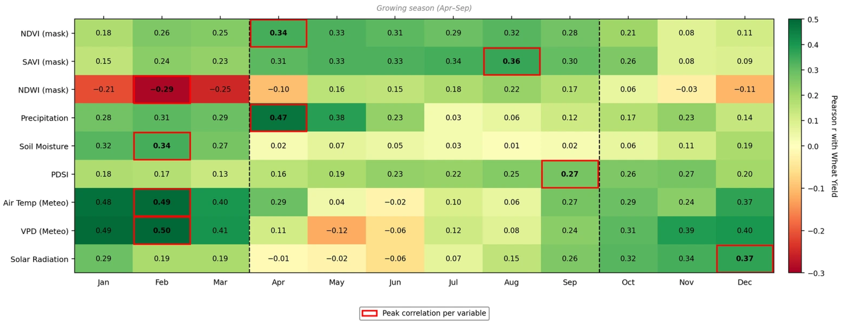
Throughout this study, “indicative cross-study comparison” refers to comparisons between results obtained in the present dataset under one experimental condition and results from external published studies under different conditions. Such comparisons indicate directionality but are not statistically controlled for methodological differences. The April NDVI–yield correlation improvement of +119.7% (r: 0.147 → 0.323; Table 4, Figure 4) and the internal SAR improvement of ΔR² = +0.052 (R²: 0.404 unmasked → 0.456 masked; +12.9% relative; within-dataset GroupKFold, 2016–2024 subset) document that 10 m cropland masking substantially improves the quality of the remote sensing (RS) predictor set in Kazakhstan. These magnitudes exceed those reported by Liu et al. [33] for Ontario, Canada (+12% for winter wheat), where the higher mean cropland fraction (~68%) limits the potential gain. Zhang et al. [63] demonstrated that masking improvements are systematically largest in regions where crops are “sparsely distributed or clustered”—precisely the condition characterising Kazakhstan’s administrative districts (mean cropland fraction ~35%, interquartile range ≈10–57%). Becker-Reshef et al. [64] further established that even approximate prior-season crop-type masks substantially improve forecast accuracy when annually updated products are unavailable, reinforcing the operational value of any masking strategy over none.

The SAR masking effect has a distinct physical basis from the optical case. VH cross-polarised C-band backscatter from urban structures, open water bodies, and rocky terrain is not simply noise—it actively antagonises the volume-scattering signal characteristic of crop canopies [50,65]. Masking eliminates these confounders, revealing the genuine Sentinel-1 sensitivity to wheat canopy height and structural development documented by Nasirzadehdizaji et al. [45] for multiple crop types. The finding that C-band SAR contributes only marginally at a district scale after masking (ΔR² = +0.009 in the fair 2016–2024 comparison) is consistent with Meroni et al. [27], who showed that SAR’s primary complementary value over optical data lies in cloud-obscured early-season windows—a benefit partially offset by our monthly median compositing strategy. Kalecinski et al. [28] demonstrated that SAR–optical synergy for yield estimation is strongest when SAR is used selectively for cloud-gap filling rather than as a constant predictor. The practical implication is clear: 10 m cropland masks derived from freely available products (Google Dynamic World [51]; ESA WorldCover [52]) are therefore recommended as a default preprocessing step for district-level yield studies in semi-arid regions with heterogeneous land cover and low cropland fractions. The magnitude of the benefit is expected to scale with the non-crop fraction of the target districts and should be verified empirically in each new setting.

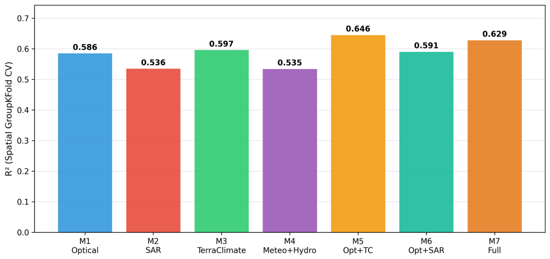
The marginal dominance of TerraClimate alone (M3: R² = 0.597) over crop-masked optical indices alone (M1: R² = 0.586)—a gap of 1.8% in relative R²—confirms the primacy of water balance in Kazakhstan’s rainfed wheat system. After proper masking, the climate–optical margin is far narrower than the 20–40% advantage reported in comparable studies at coarser resolution or without masking. Ray et al. [30] estimated that climate variation explains approximately one-third of global inter-annual crop yield variability. Our single-source climate model (R² = 0.597) substantially exceeds this theoretical ceiling, indicating that TerraClimate captures not only inter-annual climate variability but also substantial spatial productivity gradients through variables such as long-term mean precipitation and temperature that co-vary with soil quality and elevation. Hosseinpour et al. [66] observed analogous climate dominance over vegetation indices in a machine learning framework for Persian wheat, further supporting this cross-system pattern.

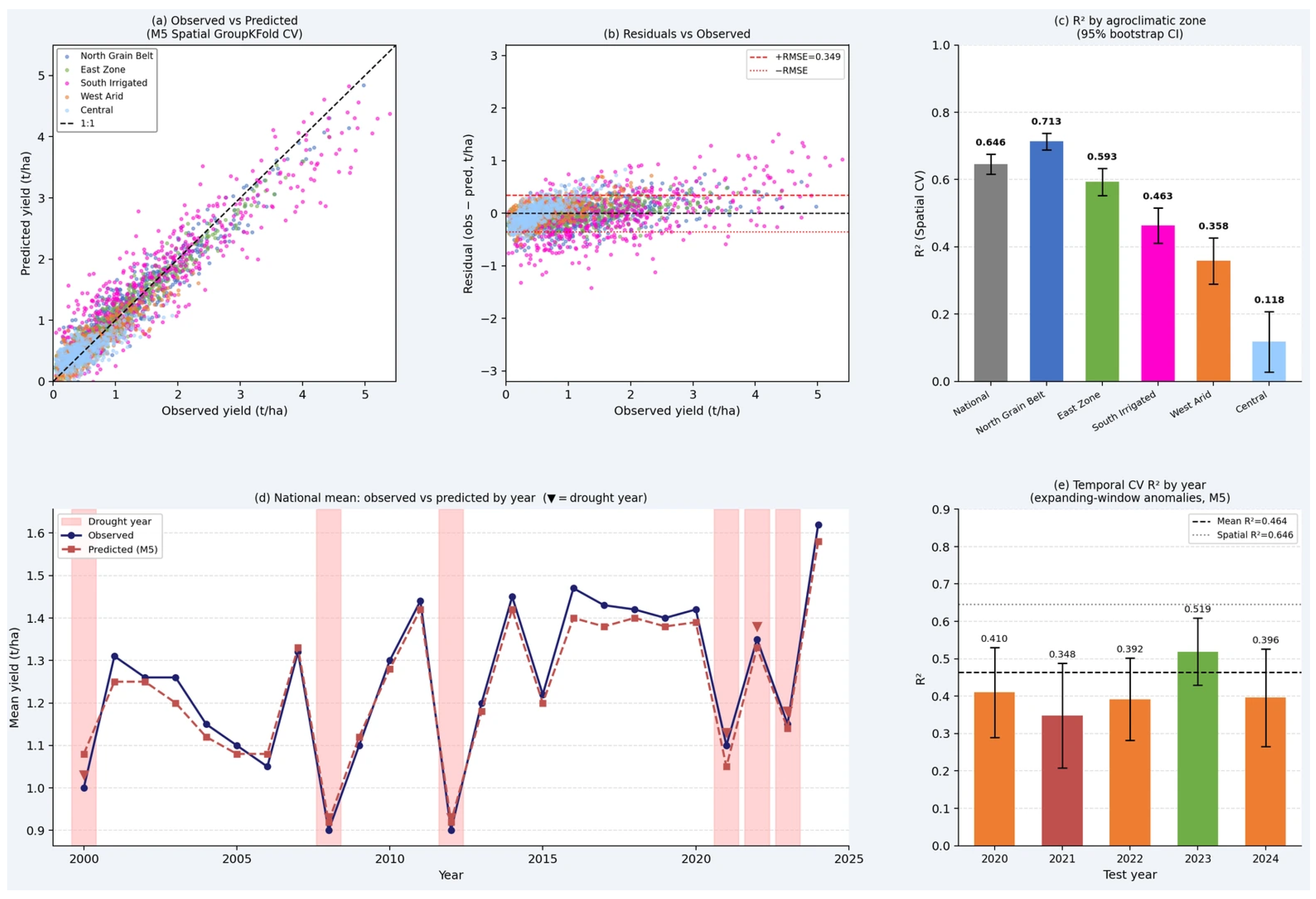
The optimal M5 configuration (optical + TerraClimate: R² = 0.646 [0.614, 0.675]; RMSE = 0.349 t/ha) confirms genuine complementarity between the two source types. TerraClimate resolves the 4 km water balance and thermal environment governing regional yield potential, while 10 m crop-masked optical indices capture sub-district heterogeneity in crop phenological timing and management intensity that gridded climate products cannot resolve. This RMSE improvement of 0.023 t/ha relative to TerraClimate alone is operationally meaningful at Kazakhstan’s scale. Cai et al. [67] reported R² ≈ 0.75 for a comparable multi-source RS + climate model in Australian dryland wheat—a higher value attributable to Australia’s larger and more homogeneous cropping zones, lower land cover heterogeneity, and potentially more favourable cross-validation design. Our M5 R² = 0.646 under geographic GroupKFold represents a conservative, spatially out-of-sample estimate directly applicable to operational early warning system design.

The underperformance of the full model (M7: R² = 0.629) relative to M5 despite incorporating SAR, meteorological station data, and soil attributes illustrates the curse of dimensionality documented by van Klompenburg et al. [15] for crop yield ML applications. With n/p ≈ 6.1 (n = 2378; p = 390), marginal sources introduce noise that partially counteracts additional information. The meteorological station model (M4: R² = 0.535) underperforming TerraClimate (M3: R² = 0.597) despite 206 vs. 157 features reflects the combined effect of 37.6% structural missingness in the KazHydroMet network and IDW interpolation errors in western districts where stations are spaced more than 200 km apart. These findings recommend that operational system design in Kazakhstan prioritise TerraClimate over sparse station networks as the primary climate predictor, supplemented by high-quality optical RS rather than station data.

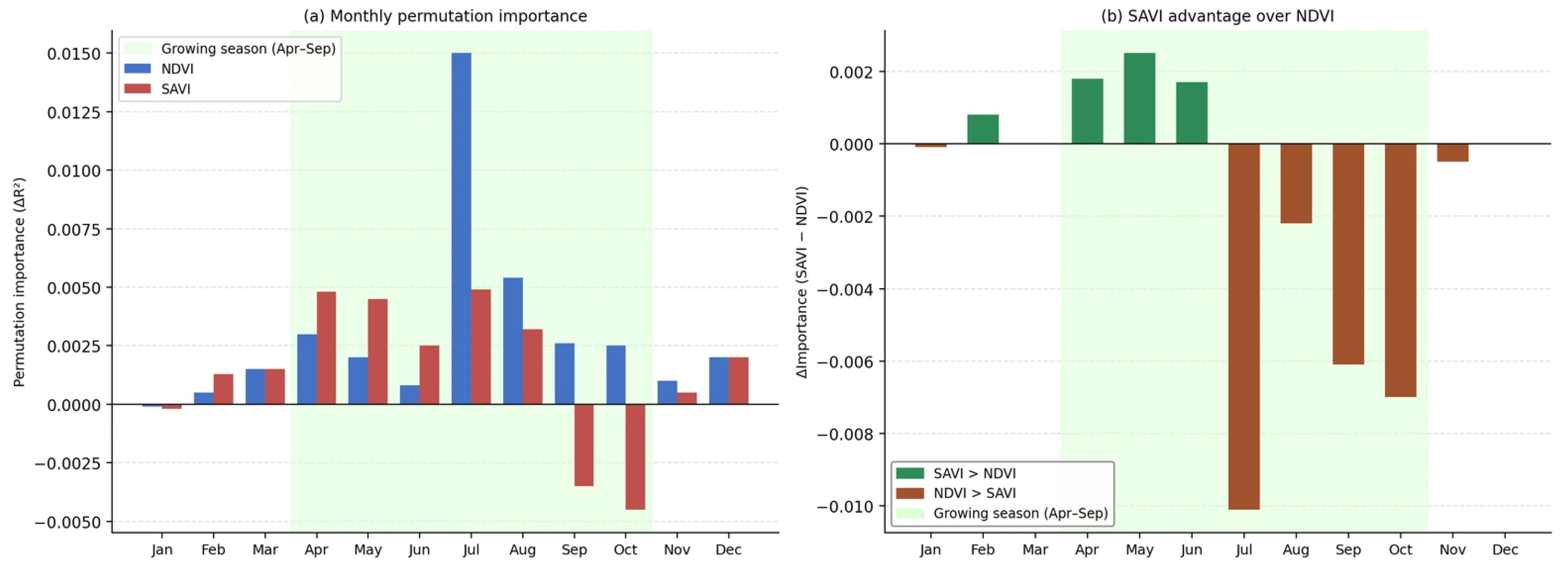
The consistent empirical superiority of SAVI over NDVI—peak r = 0.350 vs. 0.323, with the advantage growing from June (Δ = +0.02) through August (Δ = +0.027; Table 6, Figure 6)—provides comprehensive empirical validation of Huete’s [21] theoretical prediction for bright-soil, low-LAI environments. The mechanistic basis is straightforward: Kazakhstan’s calcareous soils (bare-soil ρred ≈ 0.15–0.25) create maximum soil–vegetation spectral contrast at peak canopy density (LAI ≈ 1.5–3.0 in July–August), precisely the condition where the L = 0.5 correction is most active and most beneficial. The seasonal progression—NDVI marginally superior only in April (when bare soil dominates the sparse early canopy), then SAVI gaining advantage from June through August—follows directly from this physical mechanism.

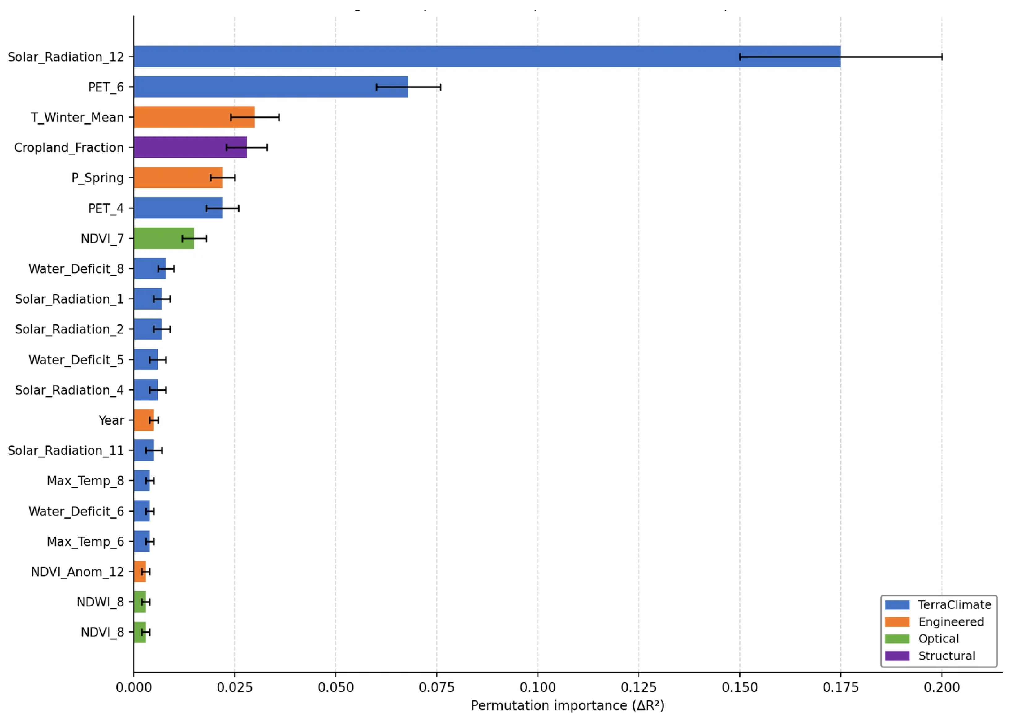
Nagy et al. [22] independently documented that SAVI substantially outperforms NDVI for wheat yield forecasting, reporting Nash–Sutcliffe efficiency E1 = 0.909 vs. 0.716 and RMSE of 0.191 vs. 0.357 t/ha for the Tisza River Catchment. Kaya and Polat [23] confirmed comparable or superior SAVI performance at post-flowering stages for winter wheat in semi-arid Turkey (Şanlıurfa province), a region with similarly bright soils. Together, these independent evaluations across three distinct agro-climatic systems—temperate European, semi-arid Mediterranean, and continental Kazakh—establish a robust cross-system evidence base for SAVI superiority in bright-soil dryland wheat applications. An important nuance, however, is that this advantage is context-dependent. In the full multi-source M5 model, NDVI_Jul (rank 7, ΔR² = 0.015) outranks SAVI_Jul (rank 15, ΔR² = 0.006) in permutation importance because the climate and cropland fraction features partially absorb the soil-brightness variance that SAVI’s correction targets. We therefore recommend SAVI as the default vegetation index for single-index correlation-based monitoring and for operational dashboards that display a single crop condition indicator. In full multi-source ML pipelines where climate data are available, both NDVI and SAVI contribute complementarily.

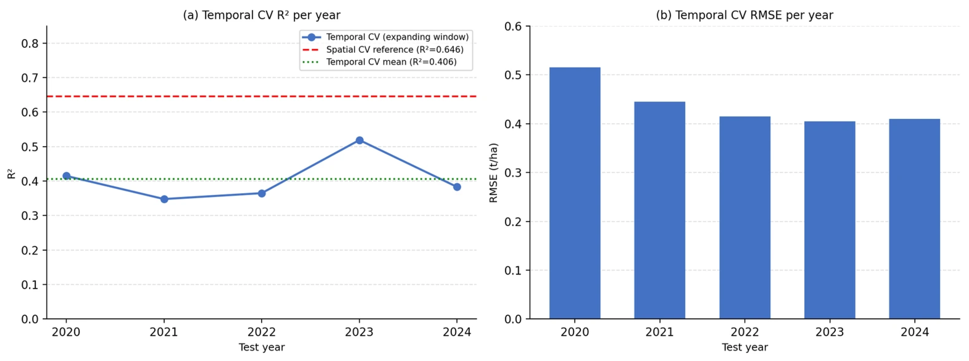
The predictability gap of ΔR² = 0.233 between spatial CV (R² = 0.646) and temporal expanding-window CV (mean R² = 0.413; Figure 12, Table 9) is the central methodological finding of this study. Roberts et al. [34] demonstrated that standard k-fold cross-validation inflates apparent accuracy for datasets with structured temporal autocorrelation because spatially separate folds still share inter-annual climate signals between training and test sets. Our observed gap is consistent with this mechanism and is particularly pronounced given Kazakhstan’s high inter-annual yield variability (CV = 0.41) driven by extreme continental climate. A decision-maker relying exclusively on spatial CV results would overestimate the operational forecast accuracy by 0.233 R² units—a magnitude sufficient to misguide resource allocation for national early warning infrastructure.

The year-to-year variation in temporal CV R² (range: 0.348–0.519) has a coherent mechanistic explanation. The worst-performing years (2021 R² = 0.348; 2022 R² = 0.392) correspond to the most severe multi-region drought since Kazakhstan’s independence, characterised by spring precipitation anomalies of −35 to −50% in the North Grain Belt with simultaneous spatial extent across all four production zones—a combination with no precedent in the 2000–2020 training data. Leng and Hall [68] documented that agricultural yield models show their largest prediction errors during concurrent multi-region drought events. They attribute this to the nonlinear physiological thresholds (below-threshold soil moisture at germination and grain fill) that statistical models systematically underrepresent due to rare occurrences in training data. Vogel et al. [69] additionally showed that the probability of such simultaneous multi-region extremes increases non-linearly with global warming. This implies that the 2021-type failure mode will become progressively more frequent under climate change, a finding with direct implications for the design of Kazakhstan’s national early warning system. The 2023 recovery year (R² = 0.519), by contrast, demonstrates that the model performs well when the test-year climate falls within the historical training distribution. We recommend that operational forecast products communicate predictive uncertainty explicitly, with wider uncertainty bounds issued in years when climate indicators suggest potential out-of-distribution conditions.

We therefore encourage the routine reporting of both spatial and temporal CV metrics in crop yield prediction studies. In our dataset, the observed gap (ΔR² = 0.233) provides an empirical benchmark for the divergence between the two protocols in a continental Central Asian wheat system. We caution, however, that this specific magnitude is dataset-dependent and should not be generalised to other systems without further evidence. Reporting only spatial CV as headline accuracy can convey an overly optimistic impression of operational forecast skill.

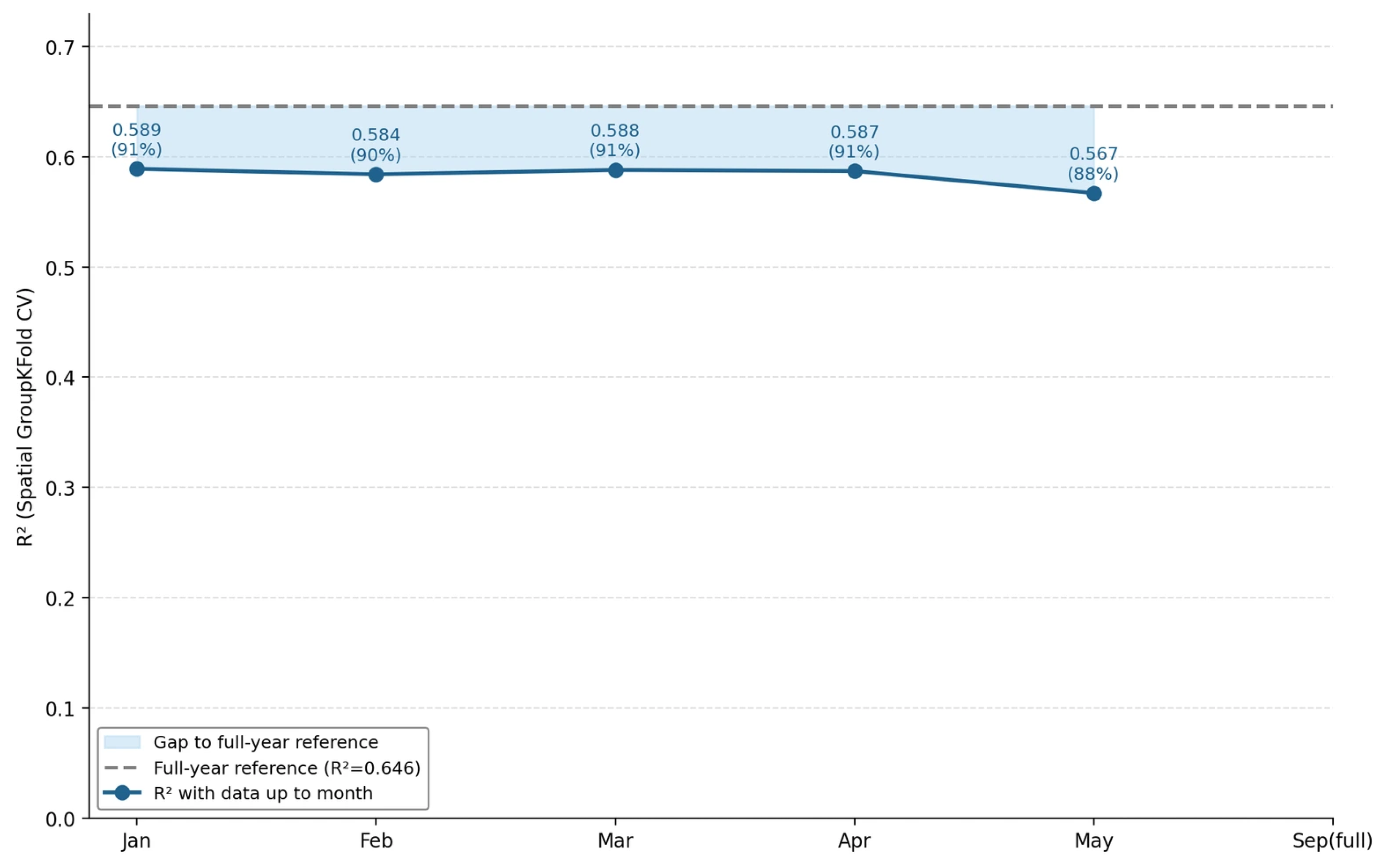
The plateau of 91% full-year accuracy using January–March data alone (R² = 0.588–0.589; Table 7, Figure 8) is among the longest pre-season forecast windows yet demonstrated for rainfed spring wheat without lagged yield predictors. The physical mechanism is rooted in Kazakhstan’s continental climate predictability structure. Years with adequate winter snowpack (captured by SWE and winter minimum temperature features) are systematically associated with adequate spring precipitation, because both are driven by the same large-scale atmospheric blocking patterns governing Central Asian winter hydrometeorology. Winter climate features therefore encode predictive information about subsequent spring conditions that are the primary wheat yield determinants, enabling reliable forecasts months before sowing.

Becker-Reshef et al. [13] demonstrated a generalised MODIS-based regression approach for winter wheat in Ukraine, achieving regression coefficients ≈ 0.74 approximately one month before harvest. This is a much shorter lead time than our January capability, attributable to winter wheat’s different phenological calendar and the absence of the winter climate–spring precipitation teleconnection relevant to spring wheat. Mkhabela et al. [14] for the Canadian Prairies reported R² = 0.48–0.90 (by zone) using June MODIS NDVI with approximately 1–2 months advance, without multi-source climate data; our multi-source framework achieving comparable accuracy 5–8 months earlier underscores the value of incorporating TerraClimate winter variables. Balaghi et al. [70] achieved R² = 0.80–0.88 for Morocco using February–April NDVI, but for a coarser spatial scale and without temporal cross-validation. The consistent finding across these systems is that pre-season climate information provides a predictability ceiling substantially higher than in-season optical observations alone in continental dryland wheat environments, motivating TerraClimate integration as the primary early-season predictor component. 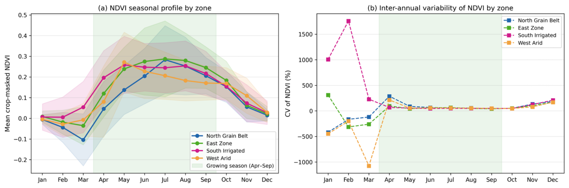The May accuracy dip (R² = 0.567, 88% of maximum) is explained by the high inter-district variability in May NDVI (CV = 0.41 vs. 0.29 in April) reflecting spatially asynchronous crop establishment. It is compounded by elevated cloud contamination (34% vs. 21% in April), which reduces the number of effective optical composites. This transient noise resolves by June as the canopy stabilises, confirming that the practical optimal forecast release window is January–April, with the June–July window adding marginal accuracy.

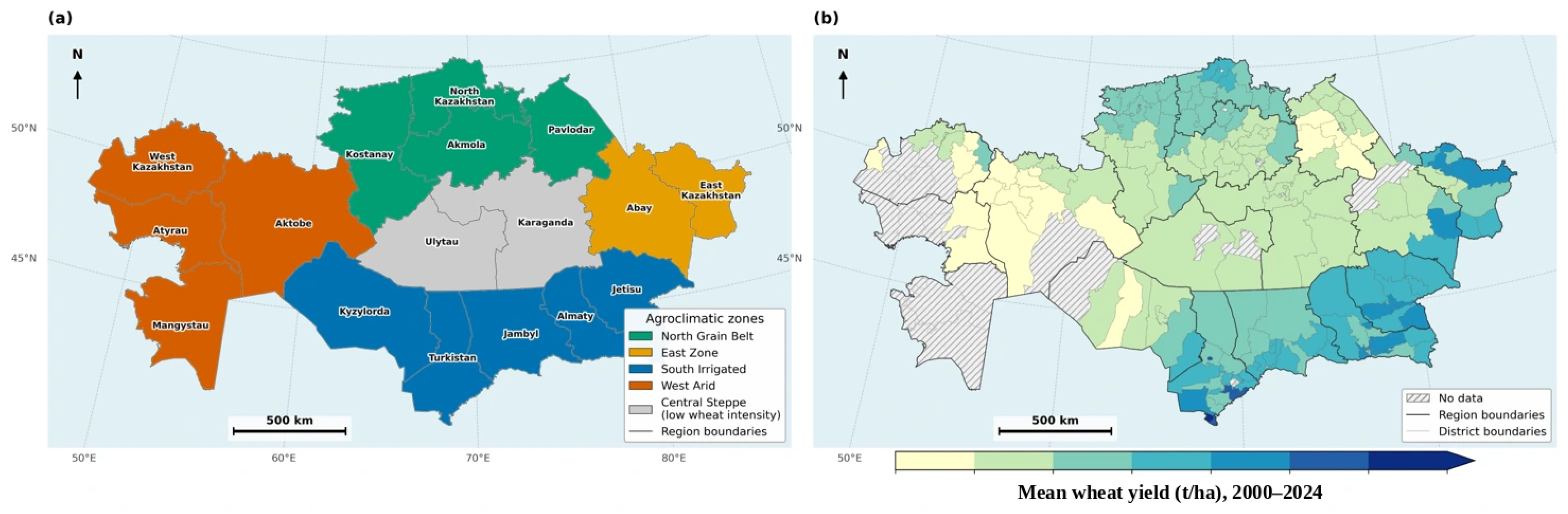
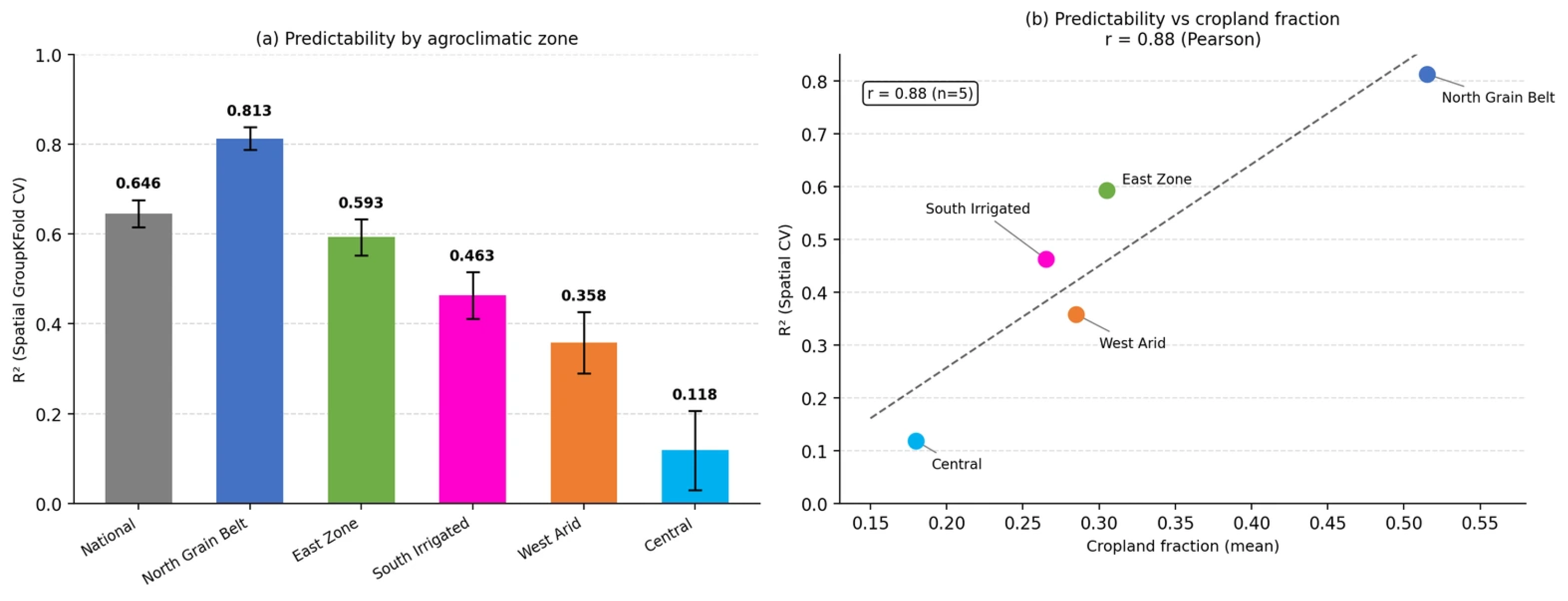
The near-perfect Pearson correlation between zone-level cropland fraction and zone-level R² (r = 0.89, n = 4; Figure 10b) quantifies a signal purity mechanism: districts with high cropland fraction (≥0.45) provide optical observations dominated by crop pixels. Districts with a low fraction (≤0.20) provide spectral means diluted by steppe, bare soil, and shrubland backgrounds even after masking. This relationship provides a predictive framework for model performance assessment without requiring model execution—a practical tool for operationalising the approach in new regions. The North Grain Belt (R² = 0.713 [0.680, 0.745]; Figure 10a) represents an ideal prediction scenario for Kazakhstan: purely rainfed spring wheat on Kazakhstan’s highest-cropland-fraction landscapes, with a short and direct precipitation–soil moisture–yield causal chain. This result exceeds the field-level predictions reported by Sadenova et al. [36] for East Kazakhstan (R² = 0.60–0.81), noting that field-level studies benefit from higher spatial resolution and absence of land cover heterogeneity, making the comparison favourable to district-level approaches.

The South Irrigated zone’s low predictability (R² = 0.463 [0.402, 0.516]; relative RMSE = 28.5%) reflects a fundamental observational gap: irrigation scheduling, canal allocation decisions, and farm management responses to in-season conditions are entirely unobservable to the model’s RS and gridded climate predictors. Lobell and Burke [31] demonstrated theoretically that decoupling soil water from precipitation through irrigation removes the dominant statistical predictor of yield variance in semi-arid systems. Arshad et al. [71] confirmed this empirically, reporting R² = 0.78 for a single intensively managed irrigated district in Punjab, Pakistan—higher than our irrigated zone average but still substantially below the rainfed North Grain Belt (R² = 0.713), consistent with the general irrigated-system predictability ceiling. Integrating water delivery records from the Syr Darya and Amu Darya irrigation systems into the model is the most promising pathway for improving South Irrigated zone predictability in future work. The Central zone’s near-zero skill (R² = 0.118 [−0.087, 0.288]) reflects the compound effect of minimal cropland fraction (0.18), extreme within-zone heterogeneity (arid Ulytau vs. temperate northern Karaganda), and insufficient training data (n = 188). This combination makes the current model configuration inappropriate for operational use in this zone.

A dedicated assessment of uncertainty sources is warranted given the multi-source, multi-decadal design. Four sources dominate. (i) Cross-sensor radiometric consistency: Because Landsat-7 ETM+ (30 m, 2000–2015) and Sentinel-2 MSI (10 m, 2016–2024) differ in spatial resolution and spectral response, crop-masked indices are not strictly comparable across the 2015/2016 transition. In the present data, mean crop-masked July NDVI is approximately 0.14 higher in the Sentinel-2 era than in the Landsat-7 era (SAVI: ~0.11 higher; Table S6)—a step substantially larger than plausible agronomic change alone and consistent with a sensor offset. The modelling framework accommodates this in three ways: the calendar year feature and the district-specific anomaly features (deviations from each district’s own climatology) absorb additive level shifts; tree-based partitioning can isolate the two regimes; and, critically, the temporal cross-validation test years (2020–2024) lie entirely within the Sentinel-2 era, so the headline operational accuracy estimates are not contaminated by cross-sensor mixing. As a robustness check, both central spectral findings reproduce within the Sentinel-2 era alone: cropland masking still raises the April NDVI–yield correlation (Δr ≈ +0.15) and SAVI still exceeds NDVI at peak canopy (Δr ≈ +0.10 in July–August; Table S7), confirming that these results are not artefacts of the sensor transition. (ii) Retrospective land-cover masking: applying the static ESA WorldCover 2021 mask to 2000–2015 could in principle distort early-period indices. However, the masking gain is of comparable magnitude within the Sentinel-2 era–where the annual Dynamic World mask is contemporaneous–as over the full period, indicating that the retrospective static mask is not the primary driver of the reported masking effect. (iii) District-level yield statistics: official rayon yields are reported as harvested production divided by harvested area, so denominator instability in drought years–when marginal area is abandoned–inflates apparent yield variability, particularly in the West Arid and Central zones. The exclusion of zero-yield and no-cultivation district–years (Section 2.2) further restricts the model to positive-production records and therefore limits its applicability to extreme area-collapse situations. This is a deliberate trade-off that favours internal statistical coherence over coverage of marginal cases, and a system intended to anticipate complete crop failure would require a separate cultivation/abandonment component. (iv) Structurally missing SAR (2000–2015): HistGradientBoosting routes missing values to whichever child node minimises the training loss at each split, so SAR features simply do not participate in predictions for pre-2016 records rather than being imputed. This motivates restricting the fair SAR assessment to the 2016–2024 overlap. The bootstrap confidence intervals reported throughout (n = 500 resamples) propagate sampling uncertainty arising from these heterogeneous completeness levels.

Several methodological limitations constrain the present findings and define a clear agenda for future work. First, the cropland mask does not distinguish wheat from other crops within agricultural pixels; a phenology-based wheat-specific classification would further improve signal purity, particularly in the South Irrigated zone where mixed cropping is common. Second, the retrospective application of ESA WorldCover 2021 as a static mask for 2000–2015 introduces potential temporal mismatch for marginal cropland dynamics, particularly in the West Arid zone where field abandonment during drought years is documented. Dynamic annual land cover products for the pre-Sentinel-2 period would address this limitation. Third, the 68% structural missingness in SAR features (2000–2015) prevents a fair full-period evaluation of SAR contribution; integrating historical ERS-2 or ENVISAT ASAR data from 1995 onward could provide a temporally balanced multi-sensor dataset. Fourth, the low predictability of the Central zone (R² = 0.118) and partial predictability of irrigated districts (R² = 0.463) reflect unobserved management variables; process-based hybrid models coupling statistical yield estimation with crop physiological constraints could improve robustness under distributional shift, particularly for unprecedented drought conditions analogous to 2021. Fifth, the feature importance hierarchy (Table 10)—dominated by December solar radiation as a spatial proxy—applies specifically to the spatial CV context. It should not be interpreted as an agronomic ranking for temporal forecasting, where pre-season winter climate variables (SWE, VPD, T_winter) would rank first. Future analyses should explicitly report spatially and temporally stratified feature importance to separate these two interpretive contexts. To summarise, the two caveats that most condition interpretation of the 25-year record are both properties of the historical input data rather than analytical choices. First, the cropland mask is retrospective: a single-year (2021) land-cover footprint was applied to the 2000–2015 period, so districts whose cultivated extent shifted over time carry a static-mask error. Second, the optical record spans a sensor transition from 30 m Landsat-7 ETM+ to 10 m Sentinel-2 MSI at 2016, introducing a systematic radiometric step (≈ +0.14 in NDVI and ≈ +0.11 in SAVI; Table S6) that exceeds plausible agronomic change. Three lines of evidence indicate that neither artefact drives our conclusions: the operational temporal-validation years (2020–2024) lie entirely within the homogeneous Sentinel-2 era; both central spectral findings—the cropland-masking gain and the SAVI-over-NDVI advantage—reproduce within that era alone (Table S7); and the cross-sensor step is absorbed by the year- and district-specific anomaly features. A fully homogeneous multi-decadal reconstruction would nonetheless require contemporaneous annual land-cover products and explicit cross-sensor radiometric harmonisation, which we identify as the principal prerequisite for extending the framework further back in time.

5. Conclusions

This study presents the first crop-masked, temporally validated, lag-free multi-source wheat yield prediction framework for Kazakhstan (149 districts, 25 years, n = 2378 modelling observations). Five principal conclusions emerge from the systematic ablation, zone-specific analysis, temporal validation, and feature importance evaluation:

• Cropland masking at 10 m resolution is essential in this low-cropland-fraction setting. Dynamic World and WorldCover masks improved NDVI–yield Pearson r by more than 100% in April and improved the masked SAR predictive R² by ΔR² = +0.052 (+12.9% relative) in a direct within-dataset masked vs. unmasked comparison (2016–2024 subset; GroupKFold, K = 3). However, a fair assessment restricted to the Sentinel-1 overlap period (n = 1093 district–years, 2016–2024; Table S3) shows no statistically significant marginal gain from adding SAR to the optical + TerraClimate configuration (M7 vs. M5: ΔR² = +0.009, overlapping CI), indicating that optical and climate data are sufficient for operational district-level yield forecasting in Kazakhstan at the current spatial resolution. Kazakhstan’s low mean district cropland fraction (~35%) amplifies the masking effect relative to other well-studied wheat-producing regions [33,63], making proper masking not a methodological refinement but a prerequisite for valid RS-based yield monitoring across the Kazakh steppe. We therefore recommend cropland masking as a default preprocessing step for district-level yield studies in semi-arid continental environments, while noting that the size of the gain is region-dependent.
• Combined optical + TerraClimate (M5) is the optimal data source configuration. M5 achieved R² = 0.646 [0.614, 0.675] and RMSE = 0.349 t/ha under spatially blocked (geographic GroupKFold) cross-validation, outperforming TerraClimate alone (R² = 0.597) and optical alone (R² = 0.586). The genuine complementarity between 4 km gridded climate data and 10 m crop-masked optical indices confirms that spring water balance and atmospheric demand—rather than peak-season canopy greenness—are the primary yield-limiting factors in Kazakhstan’s continental rainfed wheat system. TerraClimate should be co-prioritised with RS sensor quality in early warning system investment decisions.
• SAVI demonstrably outperforms NDVI in Kazakhstan’s semi-arid environment. SAVI achieved a peak Pearson r = 0.350 (August) vs. NDVI’s 0.323 (April), with the SAVI advantage growing seasonally from June (Δ = +0.02) through August (Δ = +0.027). This finding is corroborated by independent evaluations in the Tisza River Catchment [22] and semi-arid Turkey [23], establishing cross-system evidence for SAVI superiority in bright-soil dryland wheat applications. SAVI is recommended as the default vegetation index for single-index correlation-based agricultural monitoring in semi-arid environments where bright calcareous or sandy soils are present and peak LAI remains below 3.0.
• Reliable early forecasts are achievable 6–8 months before harvest. January–March data achieves 91% of full-year accuracy (R² = 0.588–0.589), driven by winter climate teleconnections (SWE, VPD, minimum temperature) that implicitly encode subsequent spring precipitation—the dominant yield determinant. The Ministry of Agriculture’s June district-level forecast requirement is met and exceeded by 4–5 months, enabling actionable advisory products for agricultural insurance pricing, fertiliser procurement, and international trade pre-contracting before sowing. This capability is operationally available today using freely accessible TerraClimate and meteorological station data, without requiring in-season satellite observations.
• Temporal CV (mean R² = 0.413) is the operationally relevant metric; spatial CV (R² = 0.646) gives a substantially more optimistic estimate, by ΔR² = 0.233 in this dataset. The 2021 severe drought (temporal R² = 0.348) exemplifies the predictive failure mode under out-of-distribution conditions: unprecedented simultaneous multi-region drought extent not represented in the training data caused systematic positive bias of 0.3–0.4 t/ha in the North Grain Belt. Reporting both spatial and temporal CV metrics is recommended as good practice. The ΔR² = 0.233 gap documented here provides a dataset-specific empirical benchmark for the divergence between the two protocols in Central Asian continental wheat systems, and explicitly communicating this gap in forecast products helps prevent overconfidence in early warning system outputs.

Together, these findings establish a reproducible, data-efficient methodological framework for district-level wheat yield prediction in semi-arid continental environments. The full pipeline relies exclusively on freely accessible satellite and gridded climate products, making it directly transferable to other Central Asian wheat-producing nations—notably Uzbekistan [37], Kyrgyzstan, and Tajikistan—where peer-reviewed district-level yield models remain absent. Future work should prioritise: (1) wheat-specific crop type classification to replace mixed-crop masks; (2) integration of irrigation water delivery records for the South Irrigated zone; (3) extension of the SAR time series using historical C-band sensors (ERS-2, ENVISAT ASAR); and (4) process-based hybrid modelling to improve robustness under unprecedented drought conditions projected to intensify under climate change [3,65].