Abstract
Hydroponic systems can drain nutrient-rich waste into the environment. Increasing irrigation efficiency would decrease effluent and improve cost efficiency for growers. However, current methods accessible to small- and mid-sized growers to determine moisture content in growth media are often imprecise. Simplified transpiration models could inform irrigation needs. This study aimed to improve transpiration estimates using vapor pressure deficit (VPD) and solar radiation. We compared our model to an existing transpiration model. Three years of transpiration and environmental data from tomato production were used to calibrate (year 2) and validate (years 1 and 3) the model. Randomly chosen subsets from all years of data were also used. The new model (TVPD) predicted the observed values more closely than the previous model (PG) in year 1 (TVPD: RMSE = 0.1570 mm, r2 = 0.95; PG: RMSE = 0.5594 to 0.6875 mm, r2 = 0.27 to 0.78) but not in year 3 (TVPD: RMSE = 0.5430 mm, r2 = 0.44; PG: RMSE = 0.1873 to 0.2065 mm, r2 = 0.95). TVPD calibrated using random subsets of the combined data improved consistency and predictive capacity (RMSE = 0.2387 to 0.2419 mm, r2 = 0.87 to 0.91). TVPD is a simpler alternative to complex models and to those focusing on solar radiation alone. TVPD is less reliable under low solar radiation (year 3); however, reliability could be improved by calibration across a broader environmental range. TVPD also allows for exploration of the relative influences of low VPD and high solar radiation on evapotranspiration found in greenhouse settings.
1. Introduction
Food producers need to feed a growing population while decreasing agricultural pollution. Food production must increase by approximately 60% by 2050 to feed a projected 9 billion global population [1,2]. At current production levels, agriculture is responsible for 70% of freshwater usage, releases nearly a third of all greenhouse gases, and is a primary pollution source for streams, lakes, and wetlands [3,4]. Steps are needed to reach food production goals while lowering negative environmental impacts. Better water management could be a key to the needed improvements.
A 2022 review of studies concerning soil moisture sensor controllers reported water savings of between 20 and 92% over production without such sensors [5]. However, in systems where drip irrigation is used, sensor data can be difficult to interpret because of uneven watering throughout the soil or growing media [6,7]. Measurement variability can also be a problem with sensors. For example, Nolz and Kammerer [8] reported that an average of multiple sensor readings was −57 kPa, while the known matric potential was −100 kPa, and there was great variation between sensors at known matric potentials of −200 and −300 kPa. These problems can be compounded when using drip irrigation in growing media, such as coco coir, where the ratio of dust to chips in the coco coir can impact sensor readings [9].
Water usage in agricultural systems is driven by evaporation from the growing media and transpiration of water vapor through the stomatal pores of the leaf. Together, these are termed “evapotranspiration”, and both correlate strongly with environmental variables that drive water vapor flux or contribute to the opening and closing of the stomata. As such, a model relating evapotranspiration to measurable environmental factors could provide more accurate and timely water use predictions. When paired with known irrigation volumes, predicted evapotranspiration values could be used to calculate water remaining in or drained from the system and, thus, irrigation needs [10].
There are several existing models designed to produce transpiration predictions, but many of these are complex or lack accuracy [10,11], impacting their application by growers. Three transpiration models, Penman–Monteith (PM), Priestley–Taylor (PT), and Shuttleworth–Wallace (SW), were compared by Shao et al. [11], who reported strong coefficients of determination for each (r2 = 0.96 to 0.98 for PM, r2 = 0.97 to 0.98 for SW, and r2 = 0.91 to 0.98 for PT). These models are highly accurate in the conditions tested, but they are complex, and such complexity could deter small producers. For instance, the main PM equation requires the latent heat of vaporization, the slope of the curve of the saturation vapor pressure versus temperature, the canopy-intercepted net radiation, the air density, the specific heat at constant pressure, the saturation vapor pressure, the actual vapor pressure, the psychrometric constant, the aerodynamic resistance, and the canopy resistance to estimate evapotranspiration [11]. Many of the components of the main equation are themselves calculated variables requiring both fixed parameters and measured values within a series of seven additional equations that would be difficult for small to medium-sized growers to gather. The canopy-intercepted net radiation is calculated using an equation requiring net radiation at the canopy level and net radiation at the growing media substrate. The latter is calculated using a second equation, which requires net radiation at canopy level, an extinction coefficient, and the leaf area index. The aerodynamic and canopy resistance equations require the height of wind measurements, the crop height, the zero plane displacement height, the crop roughness, the wind speed, the minimal stomatal resistance, the sunlit leaf area index, and an environmental stress function, which itself uses three equations to calculate the required environmental factors. SW is more complex than PM, with as many as eighteen equations, while PT is less complex with two equations. Regardless, numerous plant and environmental variables must be input, decreasing the applicability to small and mid-sized growers.
Instead of using PM to calculate evapotranspiration directly, PM can also be used to calculate a reference evapotranspiration (ETo), which is then multiplied by a crop coefficient (Kc) to arrive at a crop evapotranspiration (ETc) prediction [12,13]. The reference crop used to calculate the baseline ETc is defined as a crop of green grass with a height of 0.12 m, so the Kc value aggregates the crop’s physical and physiological differences from this reference crop, negating the need for separate physical and physiological inputs [13]. Kc values are published for various crops and stages [12], and their use could simplify the inputs needed for predictive models.
As noted above, PM is complex, but other models, such as PrHo, a simple transpiration model developed by Fernández et al. in 2001 as cited in Gallardo et al. [10] for predicting ETo, also multiply a crop coefficient by ETo to predict ETc [12,13]. Gallardo et al. [10] used PrHo, along with known levels of irrigation, to predict transpiration and the volume of solution drained from the system. PrHo requires only solar radiation and Julian day to predict transpiration by using a regression formula, offering a method that may be more attainable for small to medium-sized growers. The calculated drainage volume was the difference between irrigation volume, which was measured, and transpiration volume, which was simulated. However, so far, PrHo is less accurate than the complex evapotranspiration models PM, SW, and PT. PrHo produced strong ETc predictions (r2 = 0.78 to 0.9); however, root mean square error (RMSE) values were up to 25% of measured daily transpiration, and drainage was only moderately predicted (r2 = 0.27 to 0.47) [10]. Predictions of both ETc and drainage need improvement for a simpler model to be viable. A similar model, also requiring leaf area index (LAI), was used by Baille et al. [14]; however, we focus on the version used by Gallardo et al. [10] as it does not require this term. Here, we aim to improve on PrHo to develop a simple model accessible to small and medium-sized growers.
Transpiration is driven by leaf area and stomatal conductance, which can be difficult to measure and understand by small producers [15,16]. Measuring these factors directly requires equipment and technological expertise that can cost several thousand dollars (Meter Group, Licor). However, stomatal conductance is influenced by vapor pressure deficit (VPD) when soil moisture is not limiting [17,18]. Additionally, tomato plants are regularly pruned in greenhouse settings, causing leaf area to remain relatively consistent during the mature-fruiting stage. Thus, VPD should be a primary factor impacting transpiration. Vapor pressure deficit is calculated as the difference between the saturation vapor pressure of the air (equivalent to 100% relative humidity) and the actual vapor pressure and represents the atmospheric demand or capacity to draw water from the leaves, soil, or open water [19]. High VPD represents high evaporative demand. Transpiration increases with VPD until, in some plants, a VPD breakpoint is reached, at which point transpiration decreases due to lowered stomatal conductance [19,20,21]. The components of VPD, temperature and humidity, can be easily measured and are measurements regularly taken in greenhouses of all sizes.
Additionally, solar radiation was shown to contribute to 38 to 81 percent of transpiration, with much of the variation influenced by VPD [22]. Solar radiation has been used in several models as a transpiration driver, including TOMGRO-PrHo, a model that incorporates PrHo with a model to predict tomato growth [10,11,13]. Transpiration rate was shown very early by Martin [22] to increase with increasing average solar radiation. Thus, solar radiation combined with VPD could improve transpiration models and ultimately drainage predictions.
This study’s aim was to analyze the transpiration predictions of a model that relies on VPD and solar radiation to calculate ETo for tomatoes grown in controlled environments, such as greenhouses, with application for both hydroponic and soil-grown systems. We hypothesize that this model will produce more accurate predictions than a model using Julian day and solar radiation and that these predictions will be on par with more complex transpiration models. To do so, we modified the transpiration module used in PrHo by Gallardo et al. [10]. Ultimately, a controlled-environment grower could use sensors for temperature, humidity, and solar radiation to provide the necessary information to predict transpiration. With a known irrigation volume, hydroponic producers could also predict drainage. These predictions could be used to inform irrigation needs.
2. Materials and Methods
2.1. Model Description
2.1.1. Overview
To develop the model of transpiration based on VPD, hereafter referred to as TVPD, we isolated and modified the equations involved in calculating drainage from the equations involved in estimating NO3− concentration in the TOMGRO-PrHo model [10]. The original Gallardo et al. set of equations, derived from the PrHo portion, is, hereafter, referred to as PG. PG was based on the Julian day and solar radiation. We calibrated TVPD and PG using a single year of data extracted from the three years of data from Shao et al. [11]—this calibrated version of PG is referred to as PGc (Table 1). We then compared the capacity of TVPD, PGc, and PG using the original coefficients [10], referred to as PGg (Table 1), to predict the observed data from Shao et al. [11].

Table 1.
Model information.
2.1.2. Calculating Transpiration
Here, as in Gallardo et al. [10], crop evapotranspiration (ETc) was calculated, following Allen et al. [12], by multiplying a crop coefficient (Kc) by a reference evapotranspiration (ETo) as follows:
where Kc incorporates crop characteristics, while ETo incorporates environmental conditions.
ETc = ETo × Kc.
Growing season Kc values are published for several crops [12] and vary for initial, mid, and season end. The Kc for fall–winter tomato crops, used here and in Gallardo et al. [10], was 1.4 from the point when the canopy reached full cover, considered mid-season [12], until 31 December. To account for low-temperature influence on transpiration, Kc was calculated from 1 January to the end of February as follows [10]:
where Kc(t) is the Kc for the day in question, and Kc(t−1) is the Kc for the previous day. JD is the Julian day, sometimes called day of the year (DDA), corresponding to 1 on 1 January and 365 on 31 December. Kc decreases after 1 January (JD = 1) at a rate of 0.007 per day until the end of February (JD = 59). While calculations for Kc before full cover are available [10], only the maximum Kc at full cover and calculation of Kc after 1 January (Equation (2)) were used, as the transpiration data [11] decreases from the date of first recording on 1 November to the end of the dataset, suggesting that full cover had already been reached. Thus, we assumed full cover was reached by at least 1 November and used 1.4 as Kc from that point until 1 January, when Kc decreases (Equation (2)).
Kc(t) = Kc(t−1) − 0.007 for 1 < JD < 59
2.1.3. Detail of the PG Module
While Equations (1) and (2) above were used with both PG and TVPD, differences between the models exist in the calculation of ETo, as can be seen in Equations (3) through (5). Using an equation developed for Mediterranean greenhouses, Gallardo et al. [10] calculated ETo in the following way:
where a1, a2, b1, and b2 are empirical coefficients and JD is the Julian day. Gallardo et al. [10] used JD as a proxy for seasonal temperature evolution [23], and the relationship between solar radiation and ETo was modified linearly by JD. Go is outside daily solar radiation (mm d−1), and t is greenhouse transmissivity (%) [23,24]. Go was calculated as daily solar radiation (MJ m−2 d−1) divided by the latent heat of water (2.45 MJ m−2 d−1 mm−1), also called the latent heat of vaporization, and was used to translate solar radiation energy units to depths of water [10,13].
Here, we assumed that solar radiation measured inside the greenhouse [11] is equivalent to daily solar radiation multiplied by greenhouse transmissivity (t) because greenhouse transmissivity can be accounted for by taking the solar radiation data inside the greenhouse as opposed to taking the data outside and adjusting it by t [10]. Therefore, t is not used. Thus, for PGg and PGc, the equation becomes the following:
where GI (mm d−1), being inside daily solar radiation divided by the latent heat of water, replaces Go in the original equation.
2.1.4. Detail of the TVPD Module
Rather than being conditionally reliant on JD, TVPD is conditionally reliant on VPD (kPa) in calculating ETo (Table 1). Solar radiation (MJ m−2 d−1), which is RN in TVPD as opposed to Go or GI in PG, is used as an additive, in its influence on ETo, to that of VPD (Table 1). The equation becomes the following:
where c1 and c2 are empirical coefficients from calibration to minimize the root mean square error (RMSE) between observed evapotranspiration and predicted ETc. RN is the daily solar radiation inside the greenhouse (MJ m−2 d−1), PW is the pressure of water (0.00980665 kPa/mm), and LHW is the latent heat of water (2.45 MJ m−2 d−1 mm−1).
We used VPD and RN because we found both factors to be strongly correlated with evapotranspiration (Figure 1 and Figure 2) and because other studies have found similar correlations and/or used such relationships in models [19,20,21,25,26]. RN divided by LHW in Equation (5) is equivalent to GI in Equation (4).
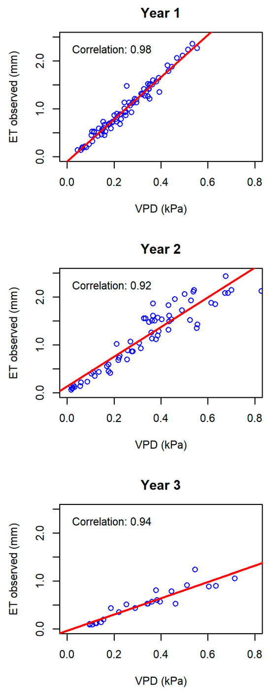
Figure 1.
Strong correlation exists between vapor pressure deficit (VPD) and evapotranspiration (ET) across the three years of data extracted from Shao et al. [11]. Blue dots indicate observed daily data points. The red line shows the fitted linear regression.
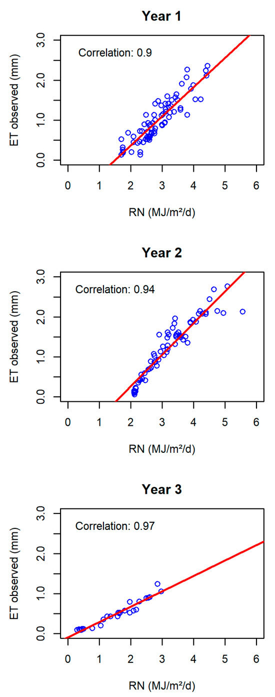
Figure 2.
Strong correlation exists between solar radiation (RN) and evapotranspiration (ET) across the three years of data extracted from Shao et al. [11]. Blue dots indicate observed daily data points. The red line shows the fitted linear regression.
2.1.5. Estimating Drainage from Transpiration Predictions
After calculating ETo using PGg (Equation (4)), PGc (Equation (4)), and TVPD (Equation (5)), ETo was multiplied by Kc (Equation (1)) to arrive at ETc [10,12]. Drainage was calculated, similarly to Gallardo et al. [10], as follows:
where DR is the predicted daily drainage (mm d−1), and IR is the daily measured irrigation (mm d−1). To overcome inconsistencies in irrigation systems, IR needs to exceed ETc by at least 20% [27]. A flowchart depicting the parameters and variables as inputs for each equation in TVPD and PG in relation to ETc and DR is depicted in Figure 3.
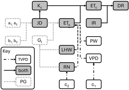
Figure 3.
The PrHo (PG) transpiration component of Gallardo et al. [10] was modified to incorporate vapor pressure deficit (VPD). This modified model was termed TVPD. For PG and TVPD, Crop Evapotranspiration (ETc) is set by the crop coefficient (Kc) and reference evapotranspiration (ETo) (Equation (1)); Kc in turn, for this model, is a conditional value set at 1.4 from mid-season until Julian day (JD) is 365 and adjusted downward daily when JD is between 1 and 59 (Equation (2)); drainage (DR) is the difference between daily irrigation (IR) and ETc (Equation (6)). For PG, ETo is modified by JD and inside daily solar radiation (GI), which is sum daily inside solar radiation (RN) divided by latent heat of water (LHW) (Equation (4)). The empirical coefficients, a1 and a2 or b1 and b2, are also used in PG (Equation (4)). For TVPD, ETo is modified by vapor pressure deficit (VPD) and the pressure of water (PW) (PW is the pressure of water in kPa/mm), along with RN and LHW (Equation (5)). The empirical coefficients, c1 and c2, are also used in TVPD.
2.1.6. Modeling Tools
Stella Professional modeling software (v3.4.1, isee systems, Lebanon, NH, USA) was used to compile and run PG and TVPD (Section S6: Figures S2 and S3, Section S1: Tables S1 and S2). All model files, parameters, and data used are freely available on Open Science Framework (OSF; https://osf.io/2g9zu/).
2.1.7. Calibration and Evaluation
The 2019 crop of Shao et al. [11], year 2 of a 3-year study, was used to calibrate PGc and TVPD. Daily transpiration, solar radiation, and VPD values were recorded, making it useful for this comparison. Briefly, tomatoes were grown in a sunken solar greenhouse at the Dacaozhuang National Breeding Experimental Station in Hebei Province, China, in a temperate continental, monsoon-influenced climate. The greenhouse floor was 1 m lower than the surrounding ground level, thus sunken, and the back wall, which faced north, was 5 m thick at the bottom, tapering to 1.2 m at the top. Transplants were planted in double rows on soil ridges covered with plastic at a density of approximately 3.5 plants per square meter, drip irrigated, and pruned. Sap flow gauges (Flow32-1K, Campbell Scientific, Logan, UT, USA) measured ETc, as has been conducted by other researchers [11,28,29]. All crops were fall–winter crops [11]. Despite having only 66 days of data, compared to 77 days for 2018 (year 1), the 2019 crop included a wider VPD range (0.02 to 0.89 kPa) and was, therefore, used for calibration. The VPD range for year 1 was 0.04 to 0.55 kPa and 0.10 to 0.71 kPa for year 3. Data for year 2 began on 1 November.
We justified this use of data from soil production for the calibration and testing of models related to hydroponic production for several reasons. First, these data were for soil production in a greenhouse with plastic-covered rows [11], which would have similarities to hydroponic systems in which plants are grown in plastic bags containing coco coir. For both, evaporation from the growing media would be limited. Second, other researchers have used models developed from data from soil production for hydroponic modeling [10,23,26,30]. The Penman–Monteith equation has regularly been used in both soil and hydroponic studies, though originally developed for soil [31,32]. Third, although it has been shown that plants grown in soil transpire at greater levels than those grown in hydroponics [33], we found a strong correlation (r = 0.99, Section S7: Figure S4) between accumulated transpiration from soil and hydroponic lettuce production using data extracted from Wang et al. [34]. While Wang et al. also found more transpiration from soil than from hydroponics, they noted that accumulated transpiration increased with time, along with plant growth, and this was shown in their study for both soil and hydroponic systems. As in Gallardo et al. [10], the calibration process, along with the use of the Kc [12,13], allows these models to be used on data from both soil and hydroponic production systems.
Calibration of PGg was conducted by Gallardo et al. [10] based on conditions in their study. They grew tomatoes (cv. ‘Tyrmex’) hydroponically using 15 L rockwool slabs and drip irrigation in a multi-span greenhouse in a Mediterranean environment in El Ejido, Spain.
Calibration of PGc and TVPD was performed using R Statistical Computing Software (v4.3.1; R Core Team 2023, Section S2) using the optim function (stats package, R Core Team 2023), which was set to minimize the RMSE between measured [11] and predicted ETc (Table 2). Predicted ETc was calculated using PGg (Equation (4)), PGc (Equation (4)), and TVPD (Equation (5)) and Equation (1). As others have found evapotranspiration to increase with VPD until a breakpoint, at which stomatal conductance decreases [19,20,21], potential breakpoints were explored using the segmented function [35] in R Statistical Computing Software and were analyzed for significance using the Davies’ test [36].
Table 2.
Equation coefficients.
The 2018 (year 1, beginning 1 November) and 2020 (year 3, beginning 14 November) fall–winter crops [11] were used for evaluating PGg, PGc, and TVPD by comparing predicted and measured transpiration using R (v4.3.1; R Core Team 2023, Section S3). For evaluation, we considered the RMSE, the coefficient of determination (r2), and bias, as well as the difference between the slope and intercept of the regressions between measured and predicted ETc relative to the 1:1 line, which were evaluated for significance with the Wald test (p < 0.05) [37]. For the evaluation of TVPD with the combined dataset, we also used K-fold cross-validation.
All data were extracted from Shao et al. [11] using PlotDigitizer (PlotDigitizer, 2023, https://plotdigitizer.com, accessed on 31 December 2024). PlotDigitizer has been shown to have a 99.1% reliability for Windows and a 99.05% reliability for macOS [38].
3. Results
3.1. Results of Calibration
TVPD Adjusted for Evapotranspiration and VPD Breakpoint
To calibrate Equation (5) using year 2 data [11], we first explored the relationships between observed evapotranspiration and VPD using both a linear and a quadratic relationship. We noted an approximately linear relationship until VPD was about 0.55 kPa (Section S4: Figure S1), after which the evapotranspiration increase rate slowed, similar to previous observations, although at a lower VPD value [39,40,41]. This lower VPD breakpoint is possible because of the high-humidity greenhouse environment and the averaging of VPD across a 24 h period. Based on this behavior, we used the segmented package [35] in R Statistical Computing Software to establish a significant VPD breakpoint, as shown in Figure 4, at 0.5 kPa (p < 0.001). The segmented package estimates breakpoints by analyzing the difference between the slopes of the regression lines on either side of the potential breakpoint, with a breakpoint existing if the absolute value of this slope difference is greater than 0 [42]. With the inclusion of the breakpoint, TVPD became conditional. The reference evapotranspiration (ETo), thus, becomes the following:
where c1 and c2 remain empirical coefficients, as in Equation (5), for minimizing, via calibration, the RMSE between observed evapotranspiration and predicted ETc when VPD < 0.5 kPa, and d1 and d2 are the corresponding empirical coefficients when VPD ≥ 0.5 kPa. As transpiration also increases with solar radiation, we explored solar radiation breakpoints instead (Section S5: Tables S3 and S4) but concluded that doing so did little to improve model predictions. Equation (7) was subsequently used for TVPD.
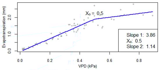
Figure 4.
A breakpoint in the data used for model calibration (year 2 of the Shao et al. [11] dataset), between VPD and evapotranspiration existed at Xo = 0.5.
3.2. Evaluation of PGg
We first evaluated PGg, which is the original PrHo model using the original parameters [10], against the three years of data extracted from Shao et al. [11]. The predicted ETc was closest to measured evapotranspiration in year 3, with an RMSE of 0.1873 mm, compared to 0.5594 mm for year 1 and 0.7455 mm for year 2 (Table 3, Figure 5). The r2 values ranged from 0.76 in year 2 to 0.95 in year 3. All regression line slopes and intercepts were significantly different from the 1:1 line (p < 0.05) (Table 3). The regression lines and bias (Table 3, Figure 5) analysis revealed mostly underprediction that increased with evapotranspiration values. In sum, PGg consistently underpredicted and had the least RMSE and greatest r2 for year 3 (Table 3, Figure 5).
Table 3.
Comparison statistics for the models over 3 years.
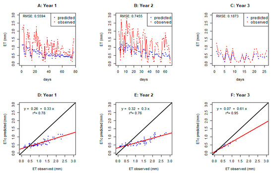
Figure 5.
PGg-predicted ETc (blue) and observed evapotranspiration (ET, red) values (mm) across the days of each year (A–C). PGg-predicted ETc and observed evapotranspiration (ET) values (mm) with the regression line (red) and the 1:1 line (black) for each year (D–F).
3.3. Evaluation of PGc
Next, we compared the performance of PGc, which is PrHo [10] calibrated using year 2 data [11]. Predicted ETc was closer to observed evapotranspiration in year 3 than in year 1 (RMSE = 0.2065 and 0.6875 mm, respectively) (Figure 6, Table 3). When compared against the calibration data from year 2, the model displayed an intermediate fit (RMSE = 0.3781 mm). Across years, the direction of bias changed. In year 1, PGc severely underpredicted evapotranspiration after day 65 but was impacted by outliers, as can be seen in Figure 6 and from the RMSE (0.6875 mm) being much greater than the mean absolute error (MAE, 0.3950 mm). For year 2, the optimized PGc tended to underpredict at low ET and overpredict at high ET, likely resulting from calibration based on minimizing RMSE. This can be seen in supplementary Section S8, Figure S5. In year 3, PGc consistently overpredicted ETc (Figure 6, Table 3). Regression line slopes and intercepts were significantly different from the 1:1 line for years 2 and 3 (p < 0.05) but not for year 1 (Table 3). The r2 values ranged from 0.27 in year 1 to 0.95 in year 3. Overall, compared to the original parameter set in PGg, optimizing the coefficients for PGc led to less accurate predictions except for the year on which the optimization was based.
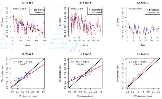
Figure 6.
PGc-predicted ETc (blue) and observed evapotranspiration (ET, red) values (mm) across the days of each year (A–C). PGc-predicted ETc and observed evapotranspiration (ET) values (mm) with the regression line (red) and the 1:1 line (black) for each year (D–F).
3.4. Evaluation of TVPD
Finally, we evaluated TVPD, the PrHo [10] modified by replacing JD with VPD. The ETc predictions by TVPD were closer to the observed evapotranspiration in year 1 than year 3 (RMSE of 0.1570 mm and 0.5430 mm, respectively) (Figure 7, Table 3). The RMSE for year 1 was also lower than for both PGg and PGc. When compared against the year 2 calibration data, TVPD again displayed an intermediate fit between years 1 and 3, although the RMSE for year 2 (RMSE = 0.1937 mm) was lower than for PGg (RMSE = 0.7455 mm) and PGc (RMSE = 0.3781 mm). In years 1 and 2, TVPD predictions track closely with measured values, having a bias of −0.0789 mm and 0.0078, respectively. In year 3, TVPD consistently overpredicts evapotranspiration, having a bias of 0.4428 (Figure 7, Table 3). The r2 values range from 0.44 in year 3 to 0.95 in year 1. The slope of the regression line in year 3 was not significantly different from that of the 1:1 line, but all other regression line slopes and intercepts were significantly different from the 1:1 line (p < 0.05) (Table 3). In sum, TVPD predictions tracked closely with measured evapotranspiration for year 1 but produced relatively large overpredictions for year 3.
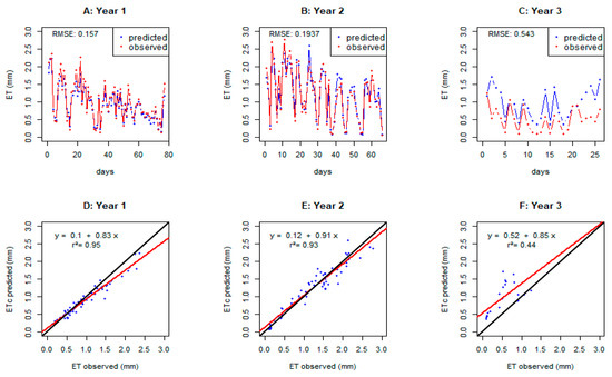
Figure 7.
TVPD-predicted ETc (blue) and observed (red) evapotranspiration (ET) values (mm) across the days of each year (A–C). TVPD-predicted ETc and observed evapotranspiration (ET) values (mm) with the regression line (red) and the 1:1 line (black) for each year (D–F).
3.5. Comparisons Among PGg, PGc, and TVPD
TVPD showed the lowest RMSE and the strongest correlation between predicted and observed evapotranspiration for years 1 and 2 (Table 3). However, the model showing the lowest RMSE for year 3 was PGg. All three models displayed some bias in the predicted results across years. Except for year 1, when all models underpredicted (PGg: −0.4155 mm, PGc: −0.1148, TVPD: −0.0789 mm), there were differences in the direction of bias across models. PGg underpredicted years 2 and 3 evapotranspiration (year 2 bias = −0.5419, year 3 bias = −0.1297), while PGc and TVPD overpredicted evapotranspiration for years 2 and 3 (PGc: year 2 bias = 0.0671, year 3 bias = 0.1837; TVPD: year 2 bias = 0.0078, year 3 bias = 0.4428). The model for which the regression line between measured and predicted values was not significantly different from the 1:1 line was PGc in year 1 (p < 0.05). However, PGc in year 1 displayed the lowest r2 of all models across all years. These PGc predictions for year 2 would likely have been improved using a larger calibration set or by the use of random subsets of the combined data, as we did for TVPD.
3.6. TVPD with No VPD Breakpoint
While the 0.5 VPD breakpoint seemed to improve the TVPD predictions relative to the PG models and provided capacity to incorporate an oft-observed stomatal response [39,40,41], there could be value in a simpler model for greenhouse settings in which the mean VPD can be low, as in the Shao et al. [11] data. Thus, we also considered TVPD with no VPD breakpoint, termed TVPD2. The results were mixed. For instance, in years 1 and 2, the RMSEs for TVPD with the breakpoint, termed TVPD1, are lower than for TVPD2, but the opposite is true for year 3 (Table 3). The r2 value for TVPD1 is greater for year 2, but lower for years 1 and 3 (Table 3). Both TVPD1 and TVPD2 underpredict in year 1 and overpredict in years 2 and 3. Bias analysis reveals similar values regardless of breakpoint use (Table 3).
3.7. Selecting a New Training Dataset
As each model showed different behaviors over each year of the dataset, we asked whether model prediction could be improved by using a subset of data pulled from across years rather than a single year. We combined the data from all three years and randomly pulled 84 days of data for calibration of TVPD1 (breakpoint, Equation (7)), leaving the remaining 85 days for evaluation. We performed this three times, using three different data randomizations. The data for each randomization were evenly selected across years, and each year’s evaluation data were approximately evenly spread along the regression line (Figure 8). Compared to our original calibration strategy, RMSE and r2 ranged between those observed for years 1 and 2 and year 3. However, both RMSE and r2 were consistent across the three calibrations, unlike with the other models and other calibration strategies. RMSE ranged from 0.2387 to 0.2419 across the calibrations (Table 4), much lower than the 0.5430 for year 3 using the original calibration strategy (Table 3). Values for r2 ranged from 0.88 to 0.91 across the three calibrations, higher than the 0.44 for year 3 using the original calibration strategy (Table 3 and Table 4). Bias analysis showed that TVPD1 using a randomized data subset for calibration consistently overpredicted for the data subset (Table 4). However, as with RMSE and r2, bias was minimal and consistent across the three calibrations, ranging from 0.0174 to 0.0530. Bias was also smaller than had been previously observed for TVPD with and without the breakpoint when compared against the evaluation sets of year 1 and year 3 (Table 3 and Table 4). The regression line was consistently different from the 1:1 line across all three randomizations, as was true in almost all years of PGg and in PGc, TVPD1, and TVPD2 calibrated using year 2. In sum, using a random subset of data spanning different years improved the consistency of model prediction. The model was also calibrated and evaluated on the combined dataset using 5-fold cross-validation, with 80% of the data being used for calibration and 20% being used for evaluation at each iteration. This resulted in less variance in the metrics (mean RMSE = 0.3024 (±0.0615) mm; mean r2 = 0.82 (±0.13); mean bias = 0.0625 (±0.0622) mm).
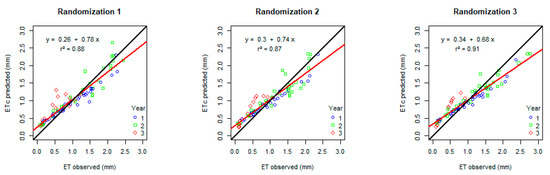
Figure 8.
Regression plots for each of the three randomizations with regression lines (red), 1:1 lines (black), and datapoints for year 1 (blue), year 2 (green), and year 3 (red).
Table 4.
Comparison Statistics for TVPD for 3 Randomly Chosen Data Subsets from All 3 Years.
3.8. Consideration of Drainage
As the purpose of our model was to improve volume drainage estimates, we next compared drainage estimates across PGg, PGc, TVPD, and with drainage estimated from Shao et al. [11]. Gallardo et al. [10] analyzed drainage from their rockwool-based, drip hydroponics system, but Shao et al. [11] used soil production with drip irrigation, providing no drainage data. For each system, drainage (DR) would simply be the difference between evapotranspiration and daily irrigation (IR) (Equation (6)), assuming, as was conducted by Gallardo et al. [10] and Shao et al. [11], that the plastic covering would cause evaporation from the growing medium to be negligible. This assumption is consistent with the observation of pepper grown in a glasshouse with and without plastic mulch [43]. Treatments with plastic mulch lost 0 mm of water to soil evaporation, while bare soil treatments lost between 18 and 255 mm to evaporation. Considering evaporation from plastic-covered soil as negligible, drainage would then be dependent on the factors that influence evapotranspiration predicted using Equations (4) and (7). In open hydroponic systems, a nutrient solution is applied at a rate that is at least 20% greater than needed, with the excess nutrient solution becoming drainage [27]. As Shao et al. [11] did not measure drainage directly, we used a value for IR that was 20% greater than the maximum observed evapotranspiration for year 1, providing an IR of approximately 2.8 mm per day. Using this IR rate, we then used each model to predict drainage for year 1 by subtracting predicted ETc from IR (Equation (6)). These values were compared to the drainage calculated from the observed transpiration values from Shao et al. [11] (Figure 9). For TVPD1, drainage values were predicted using two parameter sets: those calibrated using year 2 data from Shao et al. [11] and those calibrated using the first random set of points from the combined data. PGg and PGc used the parameters from Gallardo et al. [10] or from year 2 of Shao et al. [11], per our original design.
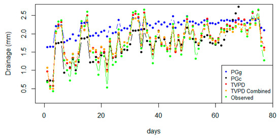
Figure 9.
Values of estimated drainage (mm) for year 1 for PGg (blue), PGc (black), TVPD1 (red), and observed (green), as well as for TVPD1 with parameters from the first randomization of the combined data (orange). These values are based on predicted ETc being subtracted from an IR of 2.8 mm. In the case of observed drainage, the observed evapotranspiration values from Shao et al. [11] were subtracted from an IR of 2.8 mm.
The RMSE values ranged from 0.1570 mm for TVPD1 to 0.6875 mm for PGc (Table 5). Values for r2 remained the same as for ETc (Table 3, Table 4 and Table 5), which is expected as the data points were simply shifted by subtracting ETc from the constant IR. Based on bias (Table 5), the models calibrated using year 2 data overpredicted but underpredicted when calibrated with the combined data. All slopes and intercepts were significantly different from those of the 1:1 line except for the slope for PGc (Table 5). The latter is due to the predictions for PGc being scattered, as can be seen in the low r2, providing a larger confidence interval for the slope, which the Wald test could not distinguish from 1. TVPD1 consistently displayed lower RMSE and bias, and higher r2 regardless of calibration method, than the PG models (Table 5). A sensitivity analysis revealed that varying the drainage fraction between 10% and 30% only changed the regression line intercept, with RMSE, bias, r2, and regression line slope remaining the same at any given drainage fraction, thus illustrating the need for a future study to directly measure drainage for comparison with predicted drainage.
Table 5.
Comparison statistics for the models for predicted drainage for year 1.
4. Discussion
We developed a transpiration model (TVPD) based on VPD and solar radiation and compared it with a model based on Julian day and solar radiation (PG). The purpose of model development was to work toward a model that could predict transpiration accurately enough to estimate drainage volumes in hydroponic systems to optimize irrigation and increase water and nutrient use efficiency. The model could be used initially as a method to predict evapotranspiration and to determine irrigation needs in both hydroponic- and soil-based controlled-environment production systems.
4.1. TVPD Model Comparison with and Without a VPD Breakpoint
We presented TVPD with and without a VPD breakpoint, which simulated the influence of decreased stomatal conductance on evapotranspiration at high VPD. The results were mixed, perhaps indicating that TVPD could improve predictions in some years or environments with very low RN, such as year 3, if the breakpoint was not used. VPD is low in humid greenhouses, perhaps leading to the effective breakpoint existing at a relatively low VPD, while a greater VPD breakpoint may be useful to simulate outdoor settings where VPD may be high. Regardless, breakpoints in previous studies were observed at higher VPD values than in the dataset used here [11]. VPD breakpoints ranged from 1.58 kPa to 2.29 kPa for maize, peanut, soybean, and cotton, although some varieties had no breakpoint [39,40,41]. For tomatoes, leaf transpiration and stomatal conductance have been shown to increase with VPD until approximately 3 kPa and 2.9 kPa, respectively, after which both begin to decrease [16]. Thus, TVPD should be tested with and without the breakpoint against other data sets from tomato crops, as well as with those from other crop species.
There is limited information concerning the response of evapotranspiration to VPD in tomatoes; however, the VPD observed by Shao et al. [11] was low relative to other studies. VPD values of 0.95 kPa, 1.6 kPa, or 2 kPa were considered low [44,45,46], compared to the 0.30 kPa mean VPD observed by Shao et al. [11]. This may be a product of how VPD was calculated, as Leonardi et al. [45] presented a VPD mean from the dryest six hours of the day, while Shao et al. [11] presented a 24 h mean. When an hourly VPD for six chosen days was presented by Shao et al. [11], the maximum VPD was between 0.5 kPa and 3.5 kPa. Thus, the observed evapotranspiration reported by Shao et al. [11] may have been influenced by VPD values that correlate with but are higher than the aggregate values reported.
The low VPD breakpoint, here, may also result from the interaction between solar radiation and VPD that can occur in greenhouse settings. Some modelers have highlighted the difficulty in reconciling the low VPD and high light intensity often observed in greenhouses [47]. As solar radiation also correlates with evapotranspiration, this suggests that an observed VPD breakpoint at a low VPD could be a product unique to greenhouses. A future study could compare VPD breakpoints in low and high VPD environments.
As TVPD incorporates both VPD and solar radiation (RN), we can explore this relationship. Comparing the modeled coefficients, which weight the relative influences of VPD and RN on reference evapotranspiration (ETo), we note that ETo is influenced more by VPD than RN until VPD values rise to at least 0.5 kPa, at which point the relationship flips (Table 2). Because the relationship in TVPD between VPD and RN is additive, the individual influence of each on ETo can be determined by dividing the coefficients by the associated constants (PW or LHW). After doing so, the weights applied to the VPD and RN components shift from 2.6327 and 0.0016 at VPD values less than 0.5 kPa to 0.8672 and 0.4619 on average at VPD values greater than 0.5 kPa, respectively. When these weights are applied to the mean VPD or RN from year 2 compiled from days on which VPD was below 0.5 kPa, the VPD component contributed 0.6772 mm (99%) to ETo, and the RN component contributed only 0.0045 mm (1%). On days when VPD was 0.5 kPa or greater, the VPD component contributed 0.5456 mm (21%), while the RN component contributed 2.0091 mm (79%) to ETo. Thus, RN might take over as the dominant factor driving ETo beyond a threshold. However, considering the high relative influence and weighting of VPD on ETo at low VPD, VPD appears to be an important component to include in a model of transpiration.
4.2. TVPD Model Performance
TVPD, as calibrated and evaluated with year 2 of the three years of annual data, performed inconsistently across years, with ETc predictions closer to observed evapotranspiration in years 1 and 2 as opposed to year 3. TVPD also outperformed PGg and PGc in years 1 and 2. However, both PG variants outperformed TVPD for year 3. Comparing TVPD with the more complex models used by Shao et al. [11] revealed that for years 1 and 2, TVPD had r2 values that fell within the range of the models of Shao et al. [11] (year 1 r2 for PM: 0.98, PT: 0.98, SW: 0.97 vs. TVPD: 0.95; year 2 r2 for PM: 0.96, PT: 0.91, SW: 0.97 vs. TVPD: 0.93). In year 3, however, the complex models used by Shao et al. [11] had greater r2 values than TVPD (r2 for PM: 0.96, PT: 0.93, SW: 0.98 vs. TVPD: 0.44). We consider four possible differences that could have contributed to the year 3 results of TVPD.
4.2.1. Differences in Year 3 ETc Values
First, year 3 has overall lower observed evapotranspiration values than year 1 or 2 (means: year 3 = 0.5046 mm, year 1 = 1.3685 mm, year 2 = 1.5989 mm; means for years 1 and 2 calculated for the first 26 days for consistency with shorter data collection period in year 3 [11]). This difference might suggest that TVPD overpredicts when evapotranspiration is low. However, when considering just the 31 lowest evapotranspiration values from year 1 (mean = 0.4965), which have a mean similar to the 26 values observed in year 3 (means = 0.5048), the RMSE and bias for the year 1 points are low while the r2 value is high, suggesting that the model performs well (year 1: RMSE = 0.0790 mm, bias = 0.0083 mm, r2 = 0.83; year 3: RMSE = 0.5430 mm, bias = 0.4428 mm, r2 = 0.44). Therefore, it is unlikely that there is a general tendency by TVPD to over-predict at low evapotranspiration.
4.2.2. Differences in Year 3 RN Values
Second, the mean RN for year 3 (1.54 MJ m−2 d−1) was less than half of that for the same days in year 1 (3.25 MJ m−2 d−1) and year 2 (3.67 MJ m−2 d−1) [11]. This might suggest a weakness in TVPD predictions at low RN levels. Comparison with days on which low RN values were observed during years 1 and 2 could not be made because there was no RN value in years 1 and 2 as small as the year 3 mean. This seems to indicate that year 3 was an abnormal year for RN. However, both PG and the complex models used by Shao et al. [11] predicted year 3 ETc with lower RMSE values and greater r2 values than TVPD. It is possible that not enough weight is given to RN by TVPD, particularly in situations where both RN and VPD are low (before the VPD breakpoint). For instance, the mean VPD (0.32 kPa) for year 3 of the Shao et al. [11] data was similar to the mean VPD for all years (0.30 kPa). If the difference was not in VPD, it is likely with RN. Secondly, when TVPD was used with no breakpoint, which gave greater weight to RN at low VPD values, r2 values for year 3 improved from 0.44 to 0.90, although RMSE values remained mostly unchanged (Table 3). Finally, as discussed in greater detail below, TVPD produced smaller RMSE values and greater r2 values when calibrated with data drawn from across the three years than when year 3 was predicted using annual data. This improvement in predictions is likely because the lower RN values from year 3 were included in the calibration data of the combined dataset but not in the year 2 calibration data. The inclusion of year 3 data in calibration led to a more balanced weighting of the RN and VPD components of TVPD at VPD values below 0.5 kPa.
4.2.3. Differences in Year 3 Fertilization
Third, fertilization amounts increased from year 1 to year 3, with N fertilization increasing from 182 kg ha−1 in year 1 to 262 kg ha−1 in year 3 and phosphorus pentoxide (P2O5) fertilization increasing from 137 kg ha−1 in year 1 to 262 kg ha−1 in year 3 [11]. These nutrient increases could have produced a more saline environment in year 3, which could decrease transpiration, as shown by Maeda et al. [48] concerning two tomato cultivars subjected to salinities of 1.2 dS m−1 and 6.0 dS m−1. At 45 DAT, they reported that ‘CF Momotaro York’ had transpiration rates of 4.5 and 3.8 mmol H2O m−2 s−1 at low and high salinity, respectively, while ‘Endeavour’ had transpiration rates of 5.7 and 4.3 mmol H2O m−2 s−1 at those salinity levels.
4.2.4. Differences in Year 3 Windspeed
Fourth, the windspeed inside the greenhouse was 0.22 m s−1 in year 1, 0.29 m s−1 in year 2, and only 0.13 m s−1 in year 3; windspeed is a factor used by many transpiration models [11,49]. Shao et al. [11] reported r2 values of greater than 0.90 for year 3 for all models analyzed and all three considered windspeed, among many other factors. While a purpose of the TVPD model is to accurately predict transpiration while requiring few inputs, a future study might consider adding windspeed as a factor for TVPD. However, adding this additional factor may not be necessary if windspeed is consistent from year to year, such as in the relatively stable microclimates produced by greenhouses where TVPD seems best suited, or if calibration data are drawn from multiple years across varying conditions.
4.3. TVPD Calibrated with Annual and Combined Datasets
The differences noted between year 3 and years 1 and 2 are likely due to the inability of TVPD, as calibrated with only year 2 data, to provide enough weighting to the RN component on days when both VPD and RN are low. PGg and PGc only consider solar radiation and Julian day but produced lower RMSE and higher r2 values for year 3 than TVPD, supporting this assertion. When year 3 data were randomly included in the calibration data, predictions improved. This suggests that TVPD predictions could be improved by the selection of more and varied calibration data.
4.4. Possible Limitations
One possible limitation of this study is that the transpiration data from Gallardo et al. [10] came from a drip hydroponics system using rockwool slabs, while the Shao et al. [11] data came from a soil production system with drip irrigation. In Shao et al. [11], the ridges on which the soil was grown were covered in plastic. We assumed that, as in the plastic-covered rockwool slabs of Gallardo et al. [10], the evaporation from the soil or growing media was negligible, and evapotranspiration from soil was strongly correlated with the same measure in a hydroponic system [34]. It is also the case that other researchers have used models developed for soil production for hydroponic production modeling [10,23,26,30]. In the future, TVPD should be evaluated in different types of growing systems and in different seasons, as well as across latitudes and altitudes.
A possible limitation of TVPD is that it requires, as do other simple transpiration models, calibration [10]. However, the need for calibration is a result of the tradeoff with complexity. TVPD can be calibrated and used in a similar production setting while requiring only two inputs, but models requiring no calibration, such as PM, need multiple inputs and employ several equations [11]. It is possible that coefficients could be calibrated for regions, production systems, and crops, allowing controlled-environment growers who produce similar crops, in similar production systems, and in similar climates to use the model without further calibration. It is also the case that breakpoints in VPD vary across plant species and cultivars and within the same species in different environments, so our specific breakpoint of 0.5 kPa may not generalize to all species and conditions and may, along with the coefficients, need calibration [16,39,40,41].
5. Conclusions
Our results suggest that TVPD could be a viable model for use in modeling transpiration and/or drainage from tomato plants grown in plastic-covered soil or plastic-wrapped substrate and using drip irrigation methods. Although the models analyzed by Shao et al. [11] had greater r2 values than TVPD in every case except one, those models required many more inputs, and thus more sensors and higher costs, than required by TVPD. It is possible to calibrate models on a single year or season of data or multiple years or seasons, which is then applied to a different season. While TVPD was limited in its predictive range when calibrated on single-year data, the model predictions improved when the calibration dataset spanned points from multiple years. As each production year can be different, even in a greenhouse setting, the use of a wide range of solar radiation and VPD data in the calibration process could be beneficial. In the future, TVPD could be immediately applied by growers by being calibrated with data from multiple seasons from other sites using similar production methods. Growers’ data could be fed back into the model each year to improve calibration over time.
Using TVPD alone, the resulting transpiration and drainage predictions could be used to inform irrigation needs in greenhouse production of tomatoes using a plastic-wrapped medium for hydroponics or plastic-covered soil. If TVPD is coupled with a nutrient model, the predicted nutrient concentration of solutions after they have passed through the system could be used to inform nutrient replenishment in closed or semi-closed hydroponic systems, as well as in open hydroponic systems.
Supplementary Materials
The following supporting information can be downloaded at: https://www.mdpi.com/article/10.3390/agronomy15092134/s1, Section S1: Table S1: Equations, Values, Parameters, and Descriptions for PG (Stella); Table S2: Equations, Values, Parameters, and Descriptions for TVPD (Stella); Section S2: R Code for Calibrating TVPD; Section S3: R Code for Evaluating TVPD; Section S4: Figure S1: Relationship between year 2 observed evapotranspiration and vapor pressure deficit (VPD), as reported in Shao et al. [11]. The red curve is the polynomial regression, the black line is the linear regression, and the blue vertical line is at 0.55 kPa. Section S5: Table S3: Comparison Statistics for TVPD with Solar Radiation Breakpoints Over Three Random Subsets of Shao et al. [11] Data; Table S4: Comparison Statistics for TVPD with Solar Radiation Breakpoints Over 3 Years of Shao et al. [11] Data; Section S6: Figure S2: The PrHo transpiration component of Gallardo et al. [10], termed PG here, was replicated for this study. In this transpiration model, “daily irrigation (IR)” flows into “drainage (DR)” at a specified “irrigation rate,” and DR is adjusted by the outflow of “evapotranspiration ETc” (Equation (6)). The rate of ETc is set by “Kc” and “reference evapotranspiration (ETo)” (Equation (1)). Kc, in turn, for this model, is set at 1.4 and adjusted downward daily by “Kc decrease” when “Julian day (JD)” is between 1 and 59 (Equation (2)). ETo is modified by both JD and “inside daily solar radiation (GI),” which is “sum daily inside solar radiation” divided by “latent heat of water (LHW)” (Equation (4)). This model was made using Stella Professional (v3.4.1, isee systems, Lebanon, NH). The bold numbers in parentheses above correspond to the equations given in the model description. Figure S3: The PrHo transpiration component of Gallardo et al. [10] was modified to incorporate vapor pressure deficit (VPD). This modified model was termed TVPD. In this evapotranspiration model, “daily irrigation (IR)” flows into “drainage (DR)” at a specified “irrigation rate,” and DR is adjusted by the outflow of “crop evapotranspiration ETc” (Equation (6)). The rate of ETc is set by the “crop coefficient (Kc)” and “reference evapotranspiration (ETo)” (Equation (1)). Kc, in turn, for this model, is set at 1.4 and adjusted downward daily by “Kc Decrease” when “Julian day (JD)” is between 1 and 59 (Equation (2)). ETo is modified by both “VPD/PW,” which is VPD divided by “pressure of water (PW)” (PW is the pressure of water in kPa/mm), and “(RN/LHW,” which is “sum daily inside solar radiation (RN)” divided by the “latent heat of water (LHW)” (Equation (5)). This model was made using Stella Professional (v3.4.1, isee systems, Lebanon, NH). The bold numbers in parentheses above correspond to the equations given in the model description. Labels in red represent changes to the PG model (Figure S2). Section S7: Figure S4: In data extracted from Wang et al. [34], water consumption by lettuce in soil and in hydroponics was strongly correlated. The soil treatment received 113 mm of water, and the hydroponic treatment had nutrient solution recirculating continuously for 11 h day−1. Section S8: Figure S5: Residuals for PGc, year 2, showing mostly underprediction below an observed ET of approximately 1.2 mm and mostly overprediction at greater observed ET.
Author Contributions
R.J.D. contributed to study conception and design, data collection, analysis and interpretation of results, and manuscript preparation. H.K.-S. advised on study design, analysis, and interpretation of results; contributed to manuscript preparation. All authors have read and agreed to the published version of the manuscript.
Funding
This material is based upon work supported by the National Science Foundation under Grant No. 2152218. Any opinions, findings, and conclusions or recommendations expressed in this material are those of the author(s) and do not necessarily reflect the views of the National Science Foundation.
Data Availability Statement
All data and codes used in the production of this work are freely available at Open Science Framework and can be accessed by the following link: https://osf.io/2g9zu/.
Acknowledgments
We acknowledge the use of ChatGPT for guidance and troubleshooting in writing R code for graphs used in this study. OpenAI (2024). ChatGPT (Version 4) [Large language model]. Retrieved from https://chat.openai.com.
Conflicts of Interest
The authors declare no conflicts of interest.
Abbreviations
The following abbreviations are used in this manuscript:
| VPD | Vapor pressure deficit |
| PM | Penman–Monteith model to predict transpiration |
| PT | Priestley–Taylor model to predict transpiration |
| SW | Shuttleworth–Wallace |
| TVPD | Transpiration model based on VPD and solar radiation |
| TVPD1 | TVPD with a VPD breakpoint |
| TVPD2 | TVPD without a VPD breakpoint |
| PGg | Model from and using parameters from Gallardo et al. [10] |
| PGc | Model from Gallardo et al. [10] recalibrated for Shao et al. [11] data |
| ETc | Calculated evapotranspiration (ETo * Kc) |
| ETo | Evapotranspiration calculated using environmental factors |
| Kc | Crop coefficient |
| JD | Julian day |
| Go | Outside solar radiation |
| t | Transmissivity |
| GI | Inside daily solar radiation |
References
- Adam, D. How far will global population rise? Researchers can’t agree. Nature 2021, 597, 462–465. [Google Scholar] [CrossRef]
- van Dijk, M.; Morley, T.; Rau, M.L.; Saghai, Y. A meta-analysis of projected global food demand and population at risk of hunger for the period. Nat. Food 2021, 2, 494–501. [Google Scholar] [CrossRef]
- International Atomic Energy Agency [IAEA]. Greenhouse Gas Reduction. Available online: https://www.iaea.org/topics/greenhouse-gas-reduction (accessed on 23 August 2023).
- Mateo-Sagasta, J.; Zadeh, S.M.; Turral, H.; Burke, J. CGIAR Research Program on Water, Land and Ecosystems (WLE). In Water Pollution from Agriculture: A Global Review—Executive Summary; FAO: Rome, Italy; International Water Management Institute (IWMI): Colombo, Sri Lanka, 2017. [Google Scholar]
- Touil, S.; Richa, A.; Fizir, M.; Argente García, J.E.; Skarmeta Gómez, A.F. A review on smart irrigation management strategies and their effect on water savings and crop yield. Irrig. Drain. 2022, 71, 1396–1416. [Google Scholar] [CrossRef]
- Amiri, Z.; Gheysari, M.; Mosaddeghi, M.R.; Amiri, S.; Tabatabaei, M.S. An attempt to find a suitable place for soil moisture sensor in a drip irrigation system. Inf. Process. Agric. 2022, 9, 254–265. [Google Scholar] [CrossRef]
- Millán, S.; Casadesús, J.; Campillo, C.; Moñino, M.J.; Prieto, M.H. Using Soil moisture sensors for automated irrigation scheduling in a plum crop. Water 2019, 11, 2061. [Google Scholar] [CrossRef]
- Nolz, R.; Kammerer, G. Evaluating a sensor setup with respect to near-surface soil water monitoring and determination of in-situ water retention functions. J. Hydrol. 2017, 549, 301–312. [Google Scholar] [CrossRef]
- Park, S.T.; Jung, G.H.; Yoo, H.J.; Choi, E.-Y.; Choi, K.-Y.; Lee, Y.-B. Measuring water content characteristics by using frequency domain reflectometry sensor in coconut coir substrate. J. Bio-Environ. Control 2014, 23, 158–166. [Google Scholar] [CrossRef]
- Gallardo, M.; Thompson, R.B.; Rodríguez, J.S.; Rodríguez, F.; Fernández, M.D.; Sánchez, J.A.; Magán, J.J. Simulation of transpiration, drainage, N uptake, nitrate leaching, and N uptake concentration in tomato grown in open substrate. Agric. Water Manag. 2009, 96, 1773–1784. [Google Scholar] [CrossRef]
- Shao, M.; Liu, H.; Yang, L. Estimating tomato transpiration cultivated in a sunken solar greenhouse with the Penman-Monteith, Shuttleworth-Wallace and Priestley-Taylor models in the North China Plain. Agronomy 2022, 12, 2382. [Google Scholar] [CrossRef]
- Allen, R.G.; Pereira, L.; Raes, D.; Smith, M. Crop Evapotranspiration: Guidelines for Computing Crop Water Requirements; Food and Agriculture Organization of the United Nations: Rome, Italy, 2000; ISBN 978-92-5-104219-9. [Google Scholar]
- Allen, R.G.; Pereira, L.; Raes, D.; Smith, M. FAO Penman-Monteith Equation. Available online: https://www.fao.org/3/X0490E/x0490e06.htm (accessed on 30 October 2023).
- Baille, M.; Baille, A.; Laury, J.C. A simplified model for predicting evapotranspiration rate of nine ornamental species vs. climate factors and leaf area. Sci. Hortic. 1994, 59, 217–232. [Google Scholar] [CrossRef]
- Bourbia, I.; Brodribb, T.J. Stomatal response to VPD is not triggered by changes in soil–leaf hydraulic conductance in arabidopsis or callitris. New Phytol. 2024, 242, 444–452. [Google Scholar] [CrossRef] [PubMed]
- Patanè, C. Leaf area index, leaf transpiration and stomatal conductance as affected by soil water deficit and vpd in processing tomato in semi arid Mediterranean climate. J. Agron. Crop Sci. 2011, 197, 165–176. [Google Scholar] [CrossRef]
- Jalakas, P.; Takahashi, Y.; Waadt, R.; Schroeder, J.I.; Merilo, E. Molecular mechanisms of stomatal closure in response to rising vapour pressure deficit. New Phytol. 2021, 232, 468–475. [Google Scholar] [CrossRef] [PubMed]
- Zhang, J.; Guan, K.; Peng, B.; Pan, M.; Zhou, W.; Jiang, C.; Kimm, H.; Franz, T.E.; Grant, R.F.; Yang, Y.; et al. Sustainable irrigation based on co-regulation of soil water supply and atmospheric evaporative demand. Nat. Commun. 2021, 12, 5549. [Google Scholar] [CrossRef]
- Grossiord, C.; Buckley, T.N.; Cernusak, L.A.; Novick, K.A.; Poulter, B.; Siegwolf, R.T.W.; Sperry, J.S.; McDowell, N.G. Plant responses to rising vapor pressure deficit. New Phytol. 2020, 226, 1550–1566. [Google Scholar] [CrossRef]
- Amitrano, C.; Rouphael, Y.; Pannico, A.; De Pascale, S.; De Micco, V. Reducing the evaporative demand improves photosynthesis and water use efficiency of indoor cultivated lettuce. Agronomy 2021, 11, 1396. [Google Scholar] [CrossRef]
- Medina, S.; Vicente, R.; Nieto-Taladriz, M.T.; Aparicio, N.; Chairi, F.; Vergara-Diaz, O.; Araus, J.L. The plant-transpiration response to vapor pressure deficit (vpd) in durum wheat is associated with differential yield performance and specific expression of genes involved in primary metabolism and water transport. Front. Plant Sci. 2019, 9, 1994. [Google Scholar] [CrossRef]
- Martin, E.V. Effect of solar radiation on transpiration of helianthus annuus. Plant Physiol. 1935, 10, 341. [Google Scholar] [CrossRef]
- Bonachela, S.; González, A.M.; Fernández, M.D. Irrigation scheduling of plastic greenhouse vegetable crops based on historical weather data. Irrig. Sci. 2006, 25, 53–62. [Google Scholar] [CrossRef]
- Linares Ojeda, R.d.M. Anejo 8. Necesidades Hídricas del Cultivo. In Proyecto de una Explotación Agrícola en el T.M. de Berja (Almería). Bachelor’s Thesis, Universidad de Almería, Repositorio de la Universidad de Almería, Almería, Spain, 2012. [Google Scholar]
- Ghimire, C.P.; van Meerveld, H.I.; Zwartendijk, B.W.; Bruijnzeel, L.A.; Ravelona, M.; Lahitiana, J.; Lubczynski, M.W. Vapour pressure deficit and solar radiation are the major drivers of transpiration in montane tropical secondary forests in eastern Madagascar. Agric. For. Meteorol. 2022, 326, 109159. [Google Scholar] [CrossRef]
- Orgaz, F.; Fernández, M.; Bonachela, S.; Gallardo, M.; Fereres, E. Evapotranspiration of horticultural crops in an unheated plastic greenhouse. Agric. Water Manag. 2005, 72, 81–96. [Google Scholar] [CrossRef]
- Kalozoumis, P.; Vourdas, C.; Ntatsi, G.; Savvas, D. Can biostimulants increase resilience of hydroponically-grown tomato to combined water and nutrient stress? Horticulturae 2021, 7, 297. [Google Scholar] [CrossRef]
- Li, X.; Zhai, J.; Sun, M.; Liu, K.; Zhao, Y.; Cao, Y.; Wang, Y. Characteristics of changes in sap flow-based transpiration of poplars, locust trees, and willows and their response to environmental impact factors. Forests 2024, 15, 90. [Google Scholar] [CrossRef]
- Navarro, A.; Scotto di Covella, F.; Cacini, S.; Sodini, M.; Traversari, S.; Venezia, A.; Massa, D. Testing sap-flow sensors to predict irrigation of soilless tomato fertigated with saline water. In Proceedings of the XXXI International Horticultural Congress (IHC2022): International Symposium on Innovative Technologies and Production 1377, Angers, France, 14–20 August 2022; pp. 639–646. [Google Scholar]
- Fernández, M.D.; Bonachela, S.; Orgaz, F.; Thompson, R.; López, J.C.; Granados, M.R.; Gallardo, M.; Fereres, E. Measurement and estimation of plastic greenhouse reference evapotranspiration in a Mediterranean climate. Irrig. Sci. 2010, 28, 497–509. [Google Scholar] [CrossRef]
- Muharomah, R.; Setiawan, B.I.; Purwanto, M.Y.J.; Liyantono, L. Temporal crop coefficients and water productivity of lettuce (lactuca sativa L.) hydroponics in planthouse. Agric. Eng. Int. CIGR J. 2020, 22, 22–29. [Google Scholar]
- Rho, H.; Su, J.; Sim, H.S.; Moon, Y.H.; Woo, U.J.; Kim, S.K. Development of a cucumber transpiration model based on a simplified Penman-Monteith model in a semi-closed greenhouse. HortScience 2023, 58, 1208–1216. [Google Scholar] [CrossRef]
- Verdoliva, S.G.; Gwyn-Jones, D.; Detheridge, A.; Robson, P. Controlled comparisons between soil and hydroponic systems reveal increased water use efficiency and higher lycopene and β-carotene contents in hydroponically grown tomatoes. Sci. Hortic. 2021, 279, 109896. [Google Scholar] [CrossRef]
- Wang, L.; Ning, S.; Zheng, W.; Guo, J.; Li, Y.; Li, Y.; Chen, X.; Ben-Gal, A.; Wei, X. Performance analysis of two typical greenhouse lettuce production systems: Commercial hydroponic production and traditional soil cultivation. Front. Plant Sci. 2023, 14, 1165856. [Google Scholar] [CrossRef]
- Muggeo, V. Interval Estimation for the Breakpoint in Segmented Regression: A smoothed score-based approach. Aust. N. Z. J. Stat. 2017, 59, 311–322. [Google Scholar] [CrossRef]
- Davies, R.B. Hypothesis testing when a nuisance parameter is present only under the alternative. Biometrika 1987, 74, 33–43. [Google Scholar]
- Wald, A.; Wolfowitz, J. An exact test for randomness in the non-parametric case based on serial correlation. Ann. Math. Stat. 1943, 14, 378–388. [Google Scholar] [CrossRef]
- Aydin, O.; Yassikaya, M.Y. Validity and reliability analysis of the PlotDigitizer software program for data extraction from single-case graphs. Perspect. Behav. Sci. 2021, 45, 239–257. [Google Scholar] [CrossRef] [PubMed]
- Broughton, K.J.; Conaty, W.C. Understanding and exploiting transpiration response to vapor pressure deficit for water limited environments. Front. Plant Sci. 2022, 13, 893994. [Google Scholar] [CrossRef]
- Devi, M.J.; Reddy, V.R. Transpiration response of cotton to vapor pressure deficit and its relationship with stomatal traits. Front. Plant Sci. 2018, 9, 1572. [Google Scholar] [CrossRef]
- Sinclair, T.R.; Devi, J.; Shekoofa, A.; Choudhary, S.; Sadok, W.; Vadez, V.; Riar, M.; Rufty, T. Limited-transpiration response to high vapor pressure deficit in crop species. Plant Sci. 2017, 260, 109–118. [Google Scholar] [CrossRef]
- Muggeo, V. Estimating regression models with unknown break-points. Stat. Med. 2003, 22, 3055–3071. [Google Scholar] [CrossRef]
- Abu-Awwad, A.M. Effect of mulch and irrigation water amounts on soil evaporation and transpiration. J. Agron. Crop Sci. 1998, 181, 55–59. [Google Scholar] [CrossRef]
- Jiao, X.-C.; Song, X.-M.; Zhang, D.-L.; Du, Q.-J.; Li, J.-M. Coordination between vapor pressure deficit and CO2 on the regulation of photosynthesis and productivity in greenhouse tomato production. Sci. Rep. 2019, 9, 8700. [Google Scholar] [CrossRef]
- Leonardi, C.; Guichard, S.; Bertin, N. High vapour pressure deficit influences growth, transpiration and quality of tomato fruits. Sci. Hortic. 2000, 84, 285–296. [Google Scholar] [CrossRef]
- Yu, X.; Niu, L.; Zhang, Y.; Xu, Z.; Zhang, J.; Zhang, S.; Li, J. Vapour pressure deficit affects crop water productivity, yield, and quality in tomatoes. Agric. Water Manag. 2024, 299, 108879. [Google Scholar] [CrossRef]
- Choi, Y.B.; Shin, J.H. Development of a transpiration model for precise irrigation control in tomato cultivation. Sci. Hortic. 2020, 267, 109358. [Google Scholar] [CrossRef]
- Maeda, K.; Johkan, M.; Tsukagoshi, S.; Maruo, T. Effect of salinity on photosynthesis and distribution of photosynthates in the Japanese tomato ‘CF Momotaro York’and the Dutch tomato ‘Endeavour’ with low node-order pinching and a high-density planting system. Hortic. J. 2020, 89, 454–459. [Google Scholar] [CrossRef]
- Katsoulas, N.; Stanghellini, C. Modelling crop transpiration in greenhouses: Different models for different applications. Agronomy 2019, 9, 392. [Google Scholar] [CrossRef]
Disclaimer/Publisher’s Note: The statements, opinions and data contained in all publications are solely those of the individual author(s) and contributor(s) and not of MDPI and/or the editor(s). MDPI and/or the editor(s) disclaim responsibility for any injury to people or property resulting from any ideas, methods, instructions or products referred to in the content. |
© 2025 by the authors. Licensee MDPI, Basel, Switzerland. This article is an open access article distributed under the terms and conditions of the Creative Commons Attribution (CC BY) license (https://creativecommons.org/licenses/by/4.0/).