How Weed Flora Evolves in Cereal Fields in Relation to the Agricultural Environment and Farming Practices in Different Sub-Regions of Eastern Hungary

Abstract

This study explores the relationship between abiotic factors, farming practices, and weed growth in winter wheat fields in Eastern Hungary. It examines the order of weed dominance and the influence of soil, environmental, and agricultural variables on weed composition and diversity before herbicide application. The research was conducted across four sub-regions in the Great Hungarian Plain, each with distinct soil, hydrological, and geographical conditions. Between 2018 and 2021, 103 fields were surveyed and weed species cover was recorded using EPPO-based identification and quadrat sampling. Soil properties, environmental conditions, and farming practices were documented through soil analysis, geographical data, and farmer interviews. Statistical analyses were preformed including ANCOVA, redundancy analysis, and Shannon diversity index calculations. The results show that common weed species include Veronica hederifolia, Stellaria media, and Apera spica-venti, with winter annuals dominating. Soil compaction and salinity affected weed diversity, while increased copper and zinc concentrations had minor effects on weed coverage. Farming practices, particularly tillage systems and fertilizer use, had a significant effect on species richness and diversity. Different regional and annual weed distributions were observed, with correlation between certain tillage systems and specific weed species. The results emphasize the need for climate-conscious farming practices, and we recommend prioritising shallow cultivation and deep loosening over ploughing in order to manage weed populations effectively. These insights contribute to sustainable weed management strategies in cereal production.

1. Introduction

Among cereals, maize and rice are the most widely cultivated, with wheat being the third most produced. Its importance is further highlighted by the fact that, after rice, it is the second most important food crop in human nutrition. According to FAOSTAT data [1], although the area of wheat cultivation has not significantly changed over recent decades, the harvested quantity has steadily increased. This, of course, is due to the increasing efficiency of farming technologies, which have required, and continue to require, intensive and ongoing agroecological research. Our research examines how weed flora and farming practices evolve in cereal fields in relation to spatial conditions in different sub-regions of Eastern Hungary.

The aim of this study was to understand and explore the effects of abiotic factors on the spread of weeds. We sought to find answers to how we can better manage the issue of weed infestation by understanding and uncovering the significance of various factors involved. Our study aimed to examine the weed composition in selected regions and assess the influence of soil, environmental, and agricultural factors on weed vegetation in cereal fields, prior to the scheduled herbicide applications in spring (19 March—8 May).

For winter wheat, which is among the most important grains, the most harmful weed species are those with life cycles similar to that of wheat, with vegetation starting in the autumn of the sowing year. Their optimal germination temperature is 10–14 °C. Winter annual weeds that germinate in the autumn and overwinter appear in the form of seedlings or rosettes (e.g., Capsella bursa-pastoris) during winter. Their life cycle is short, ending in late spring. Their damage potential is relatively low, due to their small biomass production and short life cycle. Such weed species also include Veronica spp., Lamium spp., and S. media. Although Veronica spp. have a low damage potential, they are resistant to several herbicides [2], which increases their harmfulness if they become dominant in the field. Early-germinating summer annual weeds that germinate both in autumn and spring are known as typical cereal weeds. They germinate at low temperatures, with an optimal germination temperature of 4–8 °C. During winter, they exist in the form of seedlings or seeds, and produce seeds by the time of harvest. They have a longer life cycle (Papaver rhoeas, Anthemis spp., Consolida spp.) and produce greater biomass, causing the most significant yield losses in winter wheat. Among these weeds are hard-to-control, hazardous species such as Galium aparine, A. spica-venti, and Alopecurus myosuroides. Early-summer annual weed species that germinate in spring (with an optimal germination temperature of 8–14 °C) and late-summer annual weeds that emerge in spring (with an optimal germination temperature of 18–30 °C) can also cause damage, such as Descurainia sophia and Chenopodium album. During this period, the natural senescence of winter wheat leads to a reduction in the assimilating leaf area, allowing more light to reach the lower parts of the field, which favours the development of late-emerging weed species. These weeds are typically present in wheat at the 6–8 leaf stage, but they can become more vigorous on stubble, due to more favourable living conditions [3].

Among the perennial dicotyledonous weed species that primarily reproduce vegetatively, Cirsium arvense is a significant weed, often causing localized damage by forming root colonies. Convolvulus arvensis frequently climbs onto winter wheat with its shoots. In cases of severe infestation, both weed species can hinder harvesting operations.

The changes in weed vegetation appearing in winter wheat fields can be effectively monitored based on the results of national weed surveys. In Hungary, a total of six national weed surveys have been conducted since the mid-1950s, with the aim of gaining a more detailed understanding and scientific analysis of the country’s arable weed flora. According to the most recent (sixth) national arable weed survey (2018–2019), the most significant early-spring germinating weed species in winter wheat, in order of importance, are S. media, A. spica-venti, V. hederifolia, and P. rhoeas. Special attention should be given to the remarkable spread of A. myosuroides, a particularly dangerous weed species in Western and Northern Europe due to resistance issues [4].

In spring, after the soil warms up, late-summer weed species such as Ambrosia artemisiifolia, Tripleurospermum inodorum, and Fallopia convolvulus are already causing significant weed infestations nationwide. Additionally, based on the results of surveys conducted in winter wheat fields, there is a noticeable increase in the presence of volunteer sunflower (Helianthus annuus), which can be explained by the significant expansion of sunflower cultivation areas in Hungary in recent years. As a result, volunteer sunflower is becoming an increasingly serious problem in winter wheat crops. Perennial weeds are also significant at the national level. The monocotyledonous weed Elymus repens and the dicotyledonous weeds C. arvensis and C. arvense are currently listed among the ten most important weed species. Recently, the invasion of the spreading root perennial common milkweed (Asclepias syriaca) through seed dispersal has also been observed in wheat fields [5].

Studies on the composition of weeds support the idea that environmental gradients play a key role in the composition of weed vegetation [6,7]. The number of abiotic factors affecting weed flora and its composition is quite high, making it difficult to estimate the relative importance of each factor [8].

On the other hand, farming practices such as crop types (e.g., autumn- and spring-sown crops) [9], crop rotation [10], and tillage systems [11] also play a key role in explaining changes in the species composition of weeds across large areas, which encompass a wide spectrum of soil types.

Crop rotation can reduce weed problems because the cultivation of crops with different sowing and ripening times, varying competitiveness, and different soil preparation requirements can interrupt the germination, growth, and reproduction of weed species for at least a few years [12].

Monocultures contain significantly more specialists than crop rotations, suggesting that crop rotation increases the overall species richness, rather than the pool of species specialized to individual crop types grown in the rotation [13].

The effect of the preceding crop on the weed composition of winter wheat is only apparent when herbicide use is reduced. At the same time, a significant interaction between the preceding crop and the weed density in winter wheat has been observed [14].

Andersson and Milberg [6] compared three different crop rotations. None of them had significant weed problems, and there were no clear differences in the weed flora. They concluded that when herbicides are used, the order of sowing seems less important for weed control. If a reduction or complete elimination of herbicide use is necessary, the precise composition of the crop rotation becomes much more important [15,16].

In Sussex (England), a negative correlation was observed between the abundance of broad-leaved weeds and the use of herbicides targeting dicotyledons, as well as between grass weeds and the application of broad-spectrum herbicides [17].

The impact of geographic location on the composition of weed flora is supported by several studies. Andersson and Milberg [18] studied the composition and density of weed species in Sweden. The collected data were analyzed, and the importance of the following five factors was estimated: geographic location, cultivated crop species, crop rotation, and the amount of nitrogen applied. Their results showed that geographic location has a greater impact on weed infestation than the specific crop grown on the field. This strong effect was attributed to edaphic factors. The geographical distribution of weeds is significantly influenced by atmospheric temperature, as it alters the proliferation and competitive behaviour of weeds within the crop stand [19,20].

Different weed species have varying nutrient requirements and have adapted to different nutrient availability levels, resulting in different levels of adaptability between species [21]. Similarly to cultivated crops, weed species also vary in their sensitivity to soil properties and nutrient supplementation. These factors influence the survival and spread of weeds, and highlight that weed vegetation is field-specific. Furthermore, the changes in soil properties within a field are one of the factors influencing weed infestation [22]. In soils with a high organic matter content, there is greater potential for weed species abundance and coverage compared to in soils with a low organic matter content [23].

Many weed species are more competitive than our crops because they absorb nutrients (N, P, K, Ca, and Mg) at higher concentrations. For example, species such as C. album, S. media, and T. inodorum respond intensively to high fertilizer levels, organic matter, phosphorus, potassium, and other elements [24]. In terms of the nutrients found in soil, the most limiting factor is the amount of available nitrogen, which primarily supports the growth of vegetative organs [25]. Indicator weed species that signal high concentrations of available nitrogen, according to the scales of Ellenberg [26] and Borhidi [27], include Amaranthus retroflexus, G. aparine, and Rubus caesius. These species have adapted well to intensively farmed, over-fertilized agricultural areas.

Korres et al. [28] investigated the relationship between soil physical properties and the presence of the most common weeds found in arable land. The following seven factors, in order of importance, were found to be related to the occurrence of the examined species: soil density, silt content, soil moisture content, hydraulic conductivity, wilting point, plant-available water content, and clay content. Korres et al. [28] and Kone et al. [29] found a correlation between soil nutrient content—especially phosphorus, potassium, and calcium—and the presence of broadleaf weeds. Plants generally do not prefer acidic soils with low pH values, but certain weeds may gain an advantage over crops under such conditions. Therefore, we can improve the competitiveness of our crops by adding lime [30] and/or using organic and mineral fertilization [31].

Soil salinity plays a crucial role in every stage of plant development, from germination to seed maturation [32], and it also affects water and nutrient uptake. Nutrient uptake disorders can occur, and the accumulation of certain elements, such as sodium and chloride, can be toxic to plants [33]. The genetic flexibility of weeds and their ability to adapt to unfavourable environmental conditions is high, and they generally show greater salt tolerance than cultivated plants [34].

Weed species respond quite differently to various tillage systems. As a result, the number of some species increases under reduced tillage, while the occurrence of others decreases [35]. Reduced tillage particularly favours the spread of perennial species, such as Epilobium ciliatum, Poa trivialis, C. arvense, Taraxacum officinale, Equisetum arvense, and E. repens [36]. In general, in reduced tillage systems (e.g., no-till), the soil seed bank tends to layer closer to the soil surface, while intensive tillage ensures a more uniform distribution of weed seeds throughout the depth of cultivation [37].

Several studies have demonstrated the impact of field size on weed infestation. As field size increases, a decrease in the diversity of weed flora is observed [38,39]. In smaller fields, certain farming practices may be less effective, and some weed control technologies may not be accessible to small-scale farmers, or their expertise may be insufficient at times [40].

Climate change has a significant impact on agriculture through the influence of weather factors, since they affect plant development [41]. Climate factors—primarily precipitation and temperature—play a crucial role, and these factors can vary significantly from year to year [42]. Sudden changes in weather conditions cause stress to our cultivated plants, which react sensitively and are less competitive against weeds [43]. An examination of climatic conditions in Hungary shows that these factors are significant, and among them, temperature, as a temperature-related factor, has a greater impact on weed infestation than the amount of precipitation [44,45]. The species diversity of weed flora is also related to the altitude above sea level of the site [46]. In Central Europe, the number of weed species is typically higher in higher-altitude fields. However, when studying the impact of altitude, other factors that are closely linked to climatic factors must also be considered [7]. Additionally, as the altitude increases, the number of intensively cultivated areas decreases, leading to an increase in the species diversity of the weed vegetation [47].

During our work, we have tried to find the answers to the following questions: (1) Which weed species are the most common in the winter wheat fields we studied in Eastern Hungary? (2) What are the average cover values and constancy of these weed species in the study areas? (3) How do soil, environmental, and farming variables affect the weed coverage, species richness, diversity, and weed composition of winter wheat fields?

2. Materials and Methods

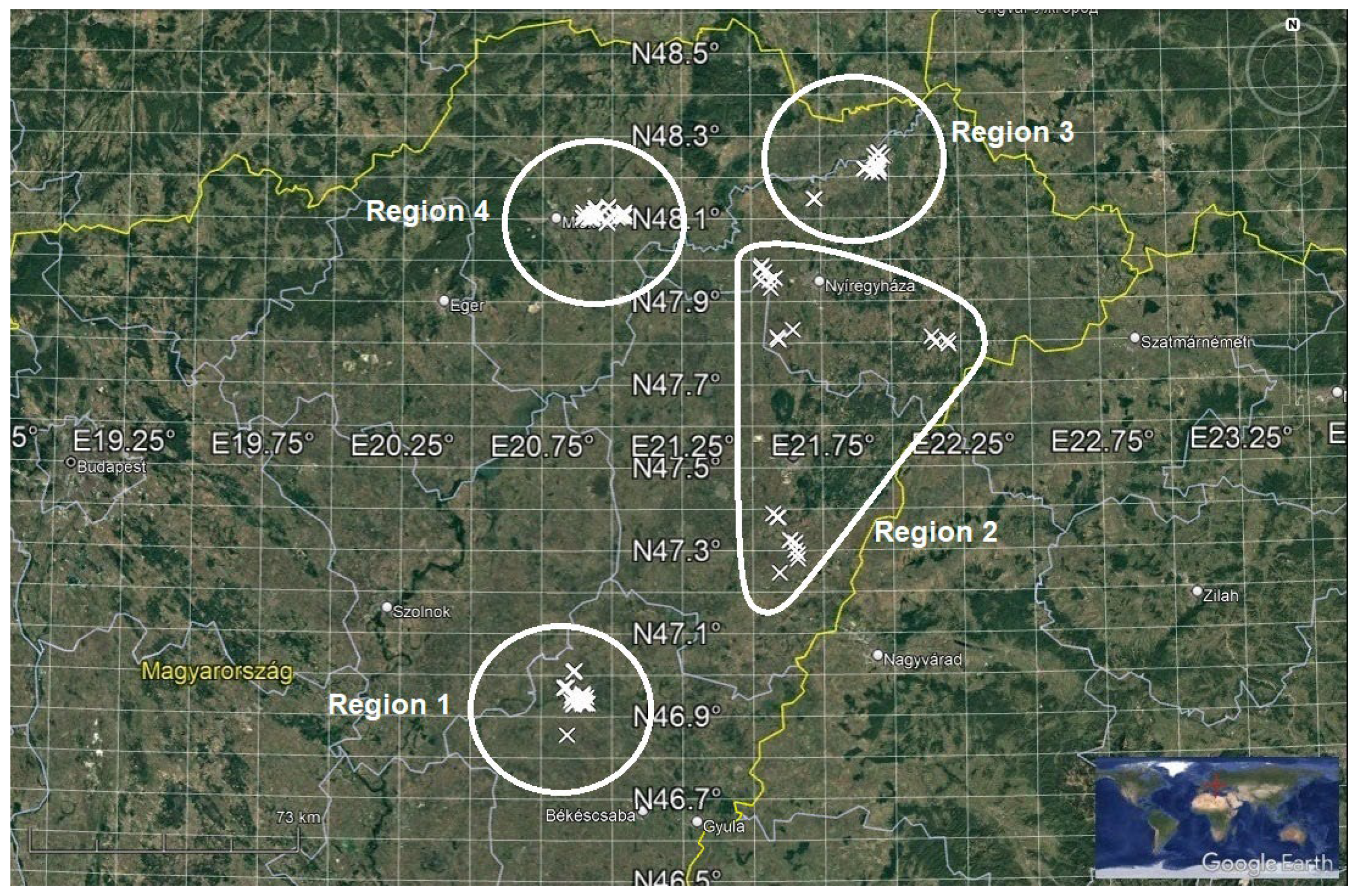
2.1. Description of the Regions Concerned

All the regions studied are characterized by a high proportion of cereal crops. The regions were selected based on soil, hydrological, and geographical (ASL) criteria, and fields with typical crop rotation, tillage, and nutrient replenishment systems were examined within each region. The location of fields surveyed in the regions is shown in Figure A1.

Region 1: This region is called the Körös Plain, and belongs to the Great Hungarian Plain macroregion, with a moderately continental climate, high groundwater levels, and a drained floodplain. It is an agricultural landscape characterized by meadow and, in some areas, saline, alluvial meadow soils. The climate is warm and dry. The region is a perfectly flat plain, with its character defined by large parcels of arable land and the woody and shrub-lined borders that divide them. The area has significantly deviated from its original natural conditions and falls into the polyhemerobic category. Due to extensive water management measures, both soil and topographical conditions have changed, and the area of natural vegetation is very limited, below 20%. The Shannon diversity index, indicating landscape usage diversity, is low, at 1.06 (compared to the national average of 1.41). The area is highly vulnerable due to natural factors, facing serious flood and waterlogging risks, as well as drought events. With the anticipated impacts of climate change, the vulnerability of current land use is expected to increase, with a high likelihood of transformation [48].

Region 2: In this region, we have grouped five micro-landscape units of similar character: Szoboszlói-Hajdúság, Hajdúhát, Löszös-Nyírség, Nagykállói-Nyírség, and Nyírbátori-Kisvárdai Nyírség. Each of them is part of the Great Hungarian Plain macroregion and is located in the Danube–Tisza Basin. They feature a moderately continental climate with gently rolling plains. The dominant soil types are loess, chernozem, humus-rich sandy soil, and drifting sand soil. The original natural conditions have been moderately altered by human activity. Intensive arable farming has further disturbed the soils, with deflation and soil compaction being characteristic. As a result, water management and oxygen supply have deteriorated. Natural vegetation is only present in 10–20% of the landscape. The Shannon index ranges between 0.61 and 1.72. The vulnerability to natural hazards is generally at a moderate level, with moderate exposure to wind erosion and drought. The risk of inland flooding is high. Due to climate change, the current land use structure may undergo moderate changes [48].

Region 3: This region includes the Rétköz microregion, which belongs to the Great Hungarian Plain macroregion as well, where the landscape is a perfect plain. The climate is dry and warm. The area is a former watercourse, slightly fragmented and poorly drained, with a reclaimed floodplain where agricultural land use dominates on meadow and floodplain soils. The natural characteristics of the landscape have primarily been influenced by water management works. The construction of dikes and canals has altered the topography, and the physical and chemical properties of the soils have been moderately modified. Natural vegetation is found in only 10–15% of the area. The Shannon diversity index, which expresses the variety of land use, is only 1.15 (compared to the national average of 1.41). The vulnerability to natural hazards is significant, as the microregion may be severely affected by floods and inland water damage. Due to climate change, it is expected that the current land use will become more vulnerable and undergo restructuring [48].

Region 4: This region includes Harangod and Sajó-Hernád sík microregions, which also belong to the Great Plain, being part of the peripheral area of the Northern Great Hungarian Plain, and extend deep into the Northern Central Mountains. A rolling plain alternates with a slight hilly influence. Its climate is moderately warm and dry. It is a loess-covered foothill area with a cone-shaped landscape, where arable land is typical, featuring moderately deep groundwater levels, with soils such as chernozem, brown forest soil, and meadow chernozem. The natural conditions have been strongly modified by human activity, resulting in a heterogeneous, mosaic-type landscape. The topography and water network have been extensively altered and regulated, with changes evident in all soil properties. Today, natural vegetation covers only 20% of the microregion. The Shannon diversity index is between 0.66 and 1.38. Due to predicted climate change, the extent and likelihood of reorganizing current land use may be moderate [48].

Meteorological data for the years and regions studied were also recorded (

Table 1. Yearly precipitation and average temperature data of surveyed regions [49].

Year A	Region 1 B		Region 2 C		Region 3 D		Region 4 E
	Rainfall (mm)	Avg. Temp. (°C)	Rainfall F (mm)	Avg. Temp. (°C)	Rainfall G (mm)	Avg. Temp. (°C)	Rainfall (mm)	Avg. Temp. (°C)
2018	737.5	11.9	643.4	10.6	699.3	10.9	618.6	10.7
2019	527.3	12.4	433.3	11.4	432.3	11.6	401.0	11.5
2020	589.8	12.3	623.4	11.0	540.9	11.5	572.4	11.2
2021	664.8	11.5	710.6	10.3	768.3	10.5	638.0	10.4
2018–2021 on average	629.9	12.0	602.7	10.8	610.2	11.1	557.5	11.0

^A Each year refers to the period between May of the previous year and April of the current year. ^B Location of data origin: Gyomaendrőd (46.9392° N, 20.8464° E). ^C Locations of data origin: Hajdúszoboszló (47.4328° N, 21.4061° E, rainfall data only), Nyírlugos (47.6961° N, 22.0569° E), and Tiszalök Arborétum (48.0256° N, 21.3044° E, rainfall data only). ^D Locations of data origin: Nagyhalász-Mága (48.0597° N, 21.7492° E, only rainfall data) and Tuzsér (48.3461° N, 22.1142° E). ^E Location of data origin: Hernádkak-Belegrád (48.0958° N, 20.9475° E). ^F Average of weather stations in Hajdószoboszló, Nyírlugos, and Tiszalök Arborétum; ^G Average of weather stations in Nagyhalász-Mága and Tuzsér.

). The distribution of precipitation varied by region, but followed a similar trend by seasons. The rainiest years were 2018 and 2021, while 2020 had average rainfall and 2019 was typically dry. The annual average temperature varied between 10.3 °C and 12.4 °C across years and regions. In all regions, the drier years corresponded to higher average temperatures. For both precipitation and average temperature, we found greater variability between years than between regions [49].

The regions share similar specificities with regard to cereal crops as the leading crops and a large intensification of production, including the use of herbicides and the unification of farming practices.

2.2. Methodology of Data Collection

In order to determine the typical weed composition in the study regions and to assess the impact of soil, environmental, and farming variables on weed vegetation, we examined a total of 103 winter wheat fields between 2018 and 2021 in four sub-regions of Eastern Hungary (between 46.858889 and 48.263222° N, 20.835611 and 22.212083° E). The scientific names of species or genera (in cases where identification at the species level was not possible, e.g., Consolida spp.) were based on the EPPO database [50]. In cases where several taxa (species) were subordinate to one species (sensu lato), the name of the polytypic species was used, e.g., V. hederifolia.

To determine weed composition, all the appearing species and their cover values, i.e., the percentage of the soil surface covered by aboveground parts of weeds [51], were recorded in eight [52] randomly placed 1 m × 1 m quadrats inside each field, ignoring a 10-metre distance from the field edges. All subsequent analyses were performed using field-level averages for all species.

Soil variables, as the most related part of the environment (referred to as ‘soil variables’ in this article), other environmental variables (referred to ‘environmental variables’), and farming variables (collectively termed ‘explanatory variables’) were recorded from soil analyses, GPS databases, or interviews with farmers for all the fields surveyed.

The dates of weed surveying (19 March–8 May) were related to the timing of chemical weed control, as species data were recorded on days 1–8 before herbicide applications, in order to show the most complete weed infestation of fields. Based on this connection, the ‘date of weed survey’ was classified as a farming variable. The dominant use of herbicides containing ALS inhibitor (HRAC group 2) and synthetic auxin (HRAC group 4) active ingredients in previous years was not included in the analysis.

The field size was also recorded, assuming that changes in the edge-to-area ratio could affect weed vegetation and management options.

The preceding crops (or vegetation) were recorded in the 3 preceding years and divided into four groups: ‘untillaged’ in the case of alfalfa or fallow; ‘spring row crops’, such as maize, sunflower, oilseed pumpkin, and watermelon; ‘cereal crops’ in the case of winter wheat, spelt wheat, triticale, and canary grass; and ‘other dense crops’ in the case of spring pea, winter pea, and winter oilseed rape. The calculation of the proportion of preceding crop groups was based on the last three years, using the following formula: (pre-crop 1 × 0.6) + (pre-crop 2 × 0.3) + (pre-crop 3 × 0.1).

The type and depth of tillage immediately preceding the assessment year were also recorded. Four types of tillage systems were used in the studied fields, including ‘disc harrowing’ at a depth of 12–16 cm, ‘shallow cultivation’ by tine cultivators at a depth of 10–25 cm, ‘ploughing’ at a depth of 20–30 cm, and ‘deep loosening’ at a depth of 30–40 cm. Both the tillage system, as a categorical variable, and the depth of tillage, as a numeric variable, were included in the analyses. Additionally, the amounts of active ingredients—N, P, and K fertilizers—applied during the growing season prior to the weed vegetation survey were also considered in the analyses (

Table 2. Ranges and units of explanatory (soil, environmental, and farming) variables.

Variable (Unit)	Range/Recorded or Calculated Values
Soil variables
Soil texture (KArany)	25–67
Soil pH (KCl)	3.65–7.20
Soil properties
Salt (m/m %)	0.01–1.13
Humus (m/m %)	0.70–3.90
N (mg kg−1)	1.0–213
P2O5 (mg kg−1)	31–931
K2O (mg kg−1)	59–604
CaCO3 (m/m %)	0.04–2.74
Na (mg kg−1)	2.5–157
Mg (mg kg−1)	27–1192
S (mg kg−1)	0.5–67.3
Cu (mg kg−1)	0.5–12.5
Mn (mg kg−1)	9–525
Zn (mg kg−1)	0.4–9.1
Environmental variables
Altitude (m, AMSL)	78–180
Latitude (° N)	46.858889–48.263222
Longitude (° E)	20.835611–22.212083
Region A	Region 1, Region 2, Region 3, Region 4
Year	2018–2021
Farming variables
Date of weed survey (Julian day)	78–128
Field size (ha)	1.5–77
Preceding crops B
Untillaged C	0–1.0
Spring row crops D	0–1.0
Cereal crops E	0–0.6
Other dense crops F	0–0.6
Tillage system	Disc harrowing, shallow cultivation, ploughing, deep loosening
Tillage depth (cm)	10–40
Amount of nitrogen fertilizer (kg a.i. ha−1)	36–168
Amount of phosphorus fertilizer (kg a.i. ha−1)	43–96
Amount of potassium fertilizer (kg a.i. ha−1)	48–110

^A The regions are described in the text. ^B The calculation based on the last three preceding crops: (pre-crop 1 × 0.6) + (pre-crop 2 × 0.3) + (pre-crop 3 × 0.1). ^C Alfalfa, fallow. ^D Maize, sunflower, oilseed pumpkin, watermelon. ^E Winter wheat, spelt wheat, triticale, canary grass. ^F Spring pea, winter pea, winter oilseed rape.

).

2.3. Data Preparation

Before the start of the analysis, the cover values of each species were aggregated within the eight plots of each field to calculate the average weed composition of each field. These field averages were subjected to a Hellinger transformation [53], and these transformed data were the basis of statistical processing.

To illustrate the overall importance of each species, both the mean cover value (without data transformation) and the constancy (field-level frequency of appearance) of each species were calculated for the fields studied.

To explore the relationship between explanatory variables, the intercorrelations were tested by the calculation of generalized variance inflation factors (GVIFs) and variance inflation factors (VIFs = GVIF ^1/(2⋅df)). In this case, we identified a close connection between regions and geographical parameters (all of altitude, latitude, and longitude), and between the tillage methods and the depth of tillage, but all measured variables were included in the statistical models to identify which of the members of the associated variable pairs had a stronger effect. In addition to this, there was also a correlation between region and soil variables (due to the fact that the delimitation of the region boundaries is partly based on soil parameters), but in these cases, the VIF values were always below 5 [54].

The Shannon diversity index was then calculated based on the distribution of (non-transformed) cover values of weed species in each field, using the following formula:

$$H’=-{\displaystyle \sum }_{i=1}^R{p}_i\ln p_i$$

where R is the number of species in each field, and p_i is the proportion of the cover values of individuals of the ith species in that field [55].

2.4. The Process of Statistical Analysis

In the first step of the statistical processing, Analyses of Covariance (ANCOVAs) were used to investigate which explanatory (soil, environmental, farming) variables significantly influenced the total weed coverage, the species richness, and the values of the calculated Shannon diversity indices, separately [56]. In cases where ANCOVAs showed a significant effect (p < 0.05), the direction and magnitude of the effect of numeric variables were tested by Pearson correlation [57]. For the assessment of correlations, absolute values of Pearson correlation coefficients between 0 and 0.19 were regarded as very weak, 0.2–0.39 as weak, 0.40–0.59 as moderate, 0.6–0.79 as strong, and 0.8–1 as very strong correlation. In the case of significant factor variables identified by ANCOVA, the differences between categories were tested with Tukey’s post hoc test [58].

In the next step, in order to describe the effect of explanatory variables on weed composition, a redundancy analysis (RDA) was carried out, using the soil, environmental, and farming variables together [RDA ref]. The set of explanatory variables was reduced by backward stepwise selection [59] using a type I error threshold of p < 0.05, resulting in a reduced model with nine variables. This step (RDA) also focused on estimating the gross and net effects of each significant explanatory variable [7], and a common ranking of ‘importance’ among all explanatory variables in this reduced model was established, based on the adjusted R² values of the net effects in the partial RDA models. To analyze the relationships between significant variables and weed species, for each partial RDA model, we identified the 10 species with the largest explained variation (fit) on the constrained axes.

All the statistical analyses were performed at the 95% significance level in the R Environment (R Development Core Team, version 4.4.2), with the use of the vegan (version: 2.6–8), permute (ver.: 0.9–7), lattice (ver.: 0.22–6), and car (ver.: 3.1–3) add-on packages.

3. Results

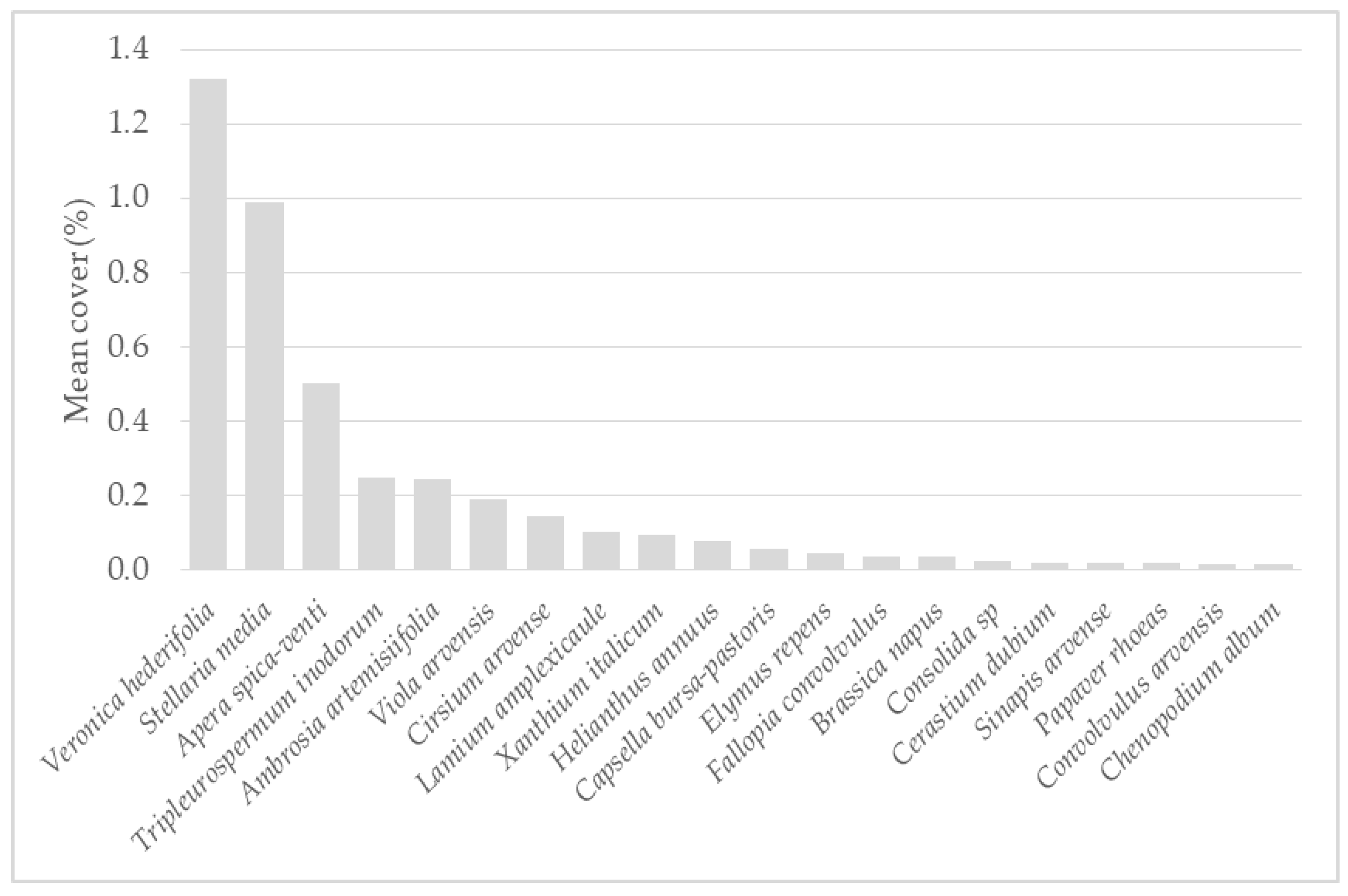
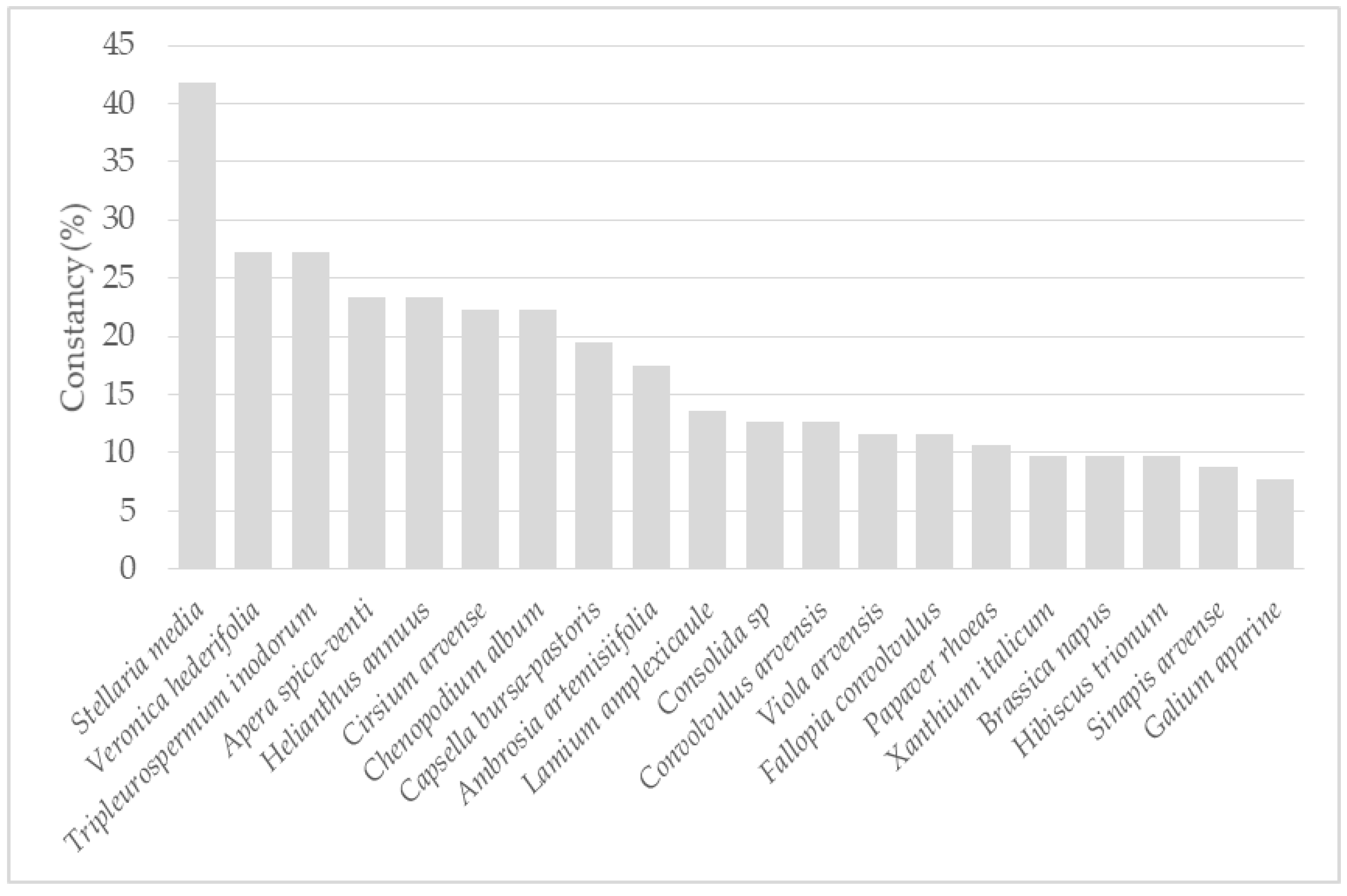
3.1. Weed Vegetation in the Regions Studied

It is visible in Figure 1 that the three most important weed species were V. hederifolia, S. media, and A. spica-venti. These three species had the highest mean cover, ranging from 0.5% to 1.3%. As observed, the most common species were winter annuals, although summer annuals were also present in the fields (e.g., T. inodorum). We also found rhizomatous perennial weeds, such as C. arvense. Furthermore, we also surveyed H. annuus and Brassica napus, as well as a negligible amount of Medicago sativa and Pisum sativum volunteers in the cereal fields. The list, taxonomic classification, predominant photosynthetic pathway, and regional distribution of all species occurring in the study area and period are given in

Table A1. The scientific name, taxonomic classification, predominant photosynthetic pathway, and regional distribution of all species occurring in the study.

Scientific Name A	Taxonomy A		Predominant Photosynthetic Pathway C	Regional Occurrence D
	Family	Class B		Region 1	Region 2	Region 3	Region 4
Amarathus retroflexus	Amaranthaceae	D	C4	x		x
Ambrosia artemisiifolia	Asteraceae	D	C3	x	x	x
Anthemis austriaca	Asteraceae	D	C3				x
Apera spica-venti	Poaceae	M	C3	x	x	x	x
Avena fatua	Poaceae	M	C3	x
Brassica napus	Brassicaceae	D	C3		x	x	x
Bromus sterilis	Poaceae	M	C3			x
Cannabis sativa	Cannabinaceae	D	C3		x	x	x
Capsella bursa-pastoris	Brassicaceae	D	C3	x	x	x	x
Cardaria draba	Brassicaceae	D	C3	x	x		x
Centaurea cyanus	Asteraceae	D	C3	x	x
Cerastium dubium	Caryophyllaceae	D	C3	x			x
Chenopodium album	Amaranthaceae	D	C3	x	x	x	x
Chenopodium hybridum	Amaranthaceae	D	C3	x			x
Chenopodium polyspermum	Amaranthaceae	D	C3	x
Cichorium intybus	Asteraceae	D	C3			x
Cirsium arvense	Asteraceae	D	C3	x	x	x	x
Consolida sp.	Ranunculaceae	D	C3	x	x	x	x
Convolvulus arvensis	Convolvulaceae	D	C3	x			x
Datura stramonium	Solanaceae	D	C3		x	x	x
Daucus carota	Apiaceae	D	C3			x
Descurainia sophia	Brassicaceae	D	C3	x	x	x	x
Elymus repens	Poaceae	M	C3			x
Fallopia convolvulus	Polygonaceae	D	C3	x	x	x	x
Fumaria schleicheri	Papaveraceae	D	C3		x
Galium aparine	Rubiaceae	D	C3	x		x	x
Helianthus annuus	Asteraceae	D	C3	x		x	x
Heliotropium europaeum	Boraginaceae	D	C3	x
Hibiscus trionum	Malvaceae	D	C3	x			x
Lactuca serriola	Asteraceae	D	C3			x
Lamium amplexicaule	Lamiaceae	D	C3	x	x	x	x
Lamium purpureum	Lamiaceae	D	C3	x		x	x
Lycopus exaltatus	Lamiaceae	D	C3		x
Medicago sativa	Fabaceae	D	C3			x
Myosurus minimus	Ranunculaceae	D	C3	x
Papaver rhoeas	Papaveraceae	D	C3	x	x	x	x
Phragmites australis	Poaceae	M	C3		x
Pisum sativum	Fabaceae	D	C3				x
Plantago lanceolata	Plantaginaceae	D	C3				x
Polygonum aviculare	Polygonaceae	D	C3	x		x
Prunus spinosa	Rosaceae	D	C3	x
Ranunculus repens	Ranunculaceae	D	C3	x		x
Raphanus raphanistrum	Brassicaceae	D	C3		x
Sinapis arvense	Brassicaceae	D	C3	x	x
Sonchus asper	Asteraceae	D	C3	x			x
Stachys annua	Lamiaceae	D	C3	x
Stellaria media	Caryophyllaceae	D	C3	x	x	x	x
Taraxacum officinale	Asteraceae	D	C3				x
Tripleurospermum inodorum	Asteraceae	D	C3	x	x	x	x
Veronica hederifolia	Scrophulariaceae	D	C3	x	x	x
Veronica polita	Scrophulariaceae	D	C3			x	x
Vicia villosa	Fabaceae	D	C3		x
Viola arvensis	Violaceae	D	C3	x		x	x
Xanthium italicum	Asteraceae	D	C3	x

^A Source: [50]. ^B M: monocotyledon, D: dicotyledon. ^C Source: [90,91,92]. ^D Region 1: Körös Plain microregion; Region 2: Szoboszlói-Hajdúság, Hajdúhát, Löszös-Nyírség, Nagykállói-Nyírség, and Nyí-rbátori-Kisvárdai Nyírség microregions; Region 3: Rétköz microregion; Region 4: Harangod and Sajó-Hernád sík microregions.

.

In terms of constancy, there were small differences compared to the ranking of weeds based on their coverage. The prevalence rate of S. media (43%) stood out. This was followed by V. hederifolia, T. inodorum, A. spica-venti, H. annuus, C. arvense, and C. album, with prevalence rates of 27, 27, 23, 23, 22, and 22%, respectively. However, a total of 15 species showed a frequency of occurrence greater than 10% (Figure 2).

3.2. The Effect of Explanatory Variables on Total Weed Coverage, Species Richness, and Diversity in the Winter Wheat Fields Surveyed

According to

Table 3. Results of ANCOVAs and Pearson correlations between variables describing weed vegetation and soil variables in winter wheat experiment (Hungary, 2018–2021).

Soil Variables	Total Weed Coverage [%]	Species Richness	Shannon Diversity
	p-values of ANCOVAs (Pearson correlation coefficients)
Soil texture	ns	<0.001 (+0.41)	<0.001 (+0.31)
Soil reaction	ns	0.025 (+0.20)	ns
Soil properties
Salt	ns	<0.001 (+0.32)	ns
Humus	ns	ns	ns
N	ns	ns	ns
P2O5	ns	ns	ns
K2O	ns	<0.001 (+0.41)	<0.001 (+0.33)
CaCO3	ns	0.041 (+0.20)	ns
Na	ns	<0.001 (+0.39)	0.001 (+0.31)
Mg	ns	<0.001 (+0.31)	0.009 (+0.25)
S	ns	<0.001 (+0.35)	0.009 (+0.26)
Cu	0.033 (+0.21)	0.024 (+0.22)	ns
Mn	ns	ns	ns
Zn	0.023 (+0.22)	<0.001 (+0.35)	0.015 (+0.24)

, soil variables had only a limited effect on total weed coverage. Based on ANCOVA and Pearson correlations, only an increase in Cu and Zn content contributed to an increase in weed coverage, to a small extent (corr.: +0.21 and +0.22).

In contrast, for the variables expressing weed diversity (species richness, Shannon diversity index), the effect of the soil conditions of the fields studied was higher. Weed composition was more complex in fields with more compact soil (corr.: +0.41 for species richness; and +0.31 for Shannon diversity index). Only soil chemistry and salinity affected species richness significantly, as a higher number of species appeared in the fields with more highly alkaline (corr.: +0.20) and highly saline (corr.: +0.32) soils. In terms of soil nutrients, the macroelement potassium and several meso- and microelements (Ca, Na, Mg, S, Cu, and Zn) influenced the weed vegetation. In all significant cases for nutrients, weak-to-moderate positive correlations were observed (corr.: +0.20–+0.41).

The results presented in

Table 4. Results of ANCOVAs, Pearson correlations (in case of significant numeric variables), and Tukey’s tests (in case of significant factor variables) on variables describing weed vegetation affected by environmental and farming variables in winter wheat experiment (Hungary, 2018–2021).

Environmental and Farming Variables	Total Weed Coverage [%]	Species Richness	Shannon Diversity
	p-values of ANCOVAs (Pearson correlation coefficients)/[mean and sign. classes of Tukey’s tests A]
Altitude	ns	0.003 (−0.29)	ns
Latitude	ns	<0.001 (−0.36)	0.017 (−0.23)
Longitude	ns	0.013 (−0.24)	ns
Region	ns	<0.001 [BEK—6.23 a HBB—2.92 b SSB—4.00 b BAZ—3.11 b]	ns
Year	0.033 [2018—5.25 a 2019—3.01 b 2020—4.31 ab 2021—4.56 ab]	<0.001 [2018—7.36 a 2019—3.61 b 2020—3.25 b 2021—2.96 b]	<0.001 [2018—1.13 a 2019—0.85 ab 2020—0.64 bc 2021—0.49 c]
Date of weed survey	ns	<0.001 (+0.42)	<0.001 (+0.34)
Field size	ns	ns	ns
Preceding crops
Undisturbed	ns	ns	ns
Spring row crops	ns	ns	ns
Cereal crops	ns	0.008 (+0.26)	0.039 (+0.20)
Other dense crops	ns	ns	ns
Tillage system  DH (disc harrowing)  SC (shallow cultivation)  PL (ploughing)  DL (deep loosening)	0.023 [DH—5.69 ab SC—1.66 c PL—9.75 a DL—1.70 bc]	0.008 [DH—5.59 a SC—3.10 b PL—3.93 ab DL—3.33 b]	ns
Tillage depth	0.006 (−0.27)	0.001 (−0.32)	0.034 (−0.13)
Amount of N fertilizer	0.011 (−0.25)	0.019 (−0.23)	ns
Amount of P fertilizer	ns	<0.001 (−0.41)	0.006 (−0.27)
Amount of K fertilizer	ns	0.023 (−0.22)	0.045 (−0.20)

^A No significant difference at the 95% confidence level between cases marked with the same letter.

show that both environmental and farming variables had a greater proportion of significant effects on species richness and Shannon diversity index than on total weed coverage. The latter was significantly affected only by the vintage, tillage system, depth of tillage, and amount of N fertilizer. Of the years surveyed, the highest weed infestation was observed in 2018 (5.25%) and the lowest in 2019 (3.01%). In the evaluation of tillage systems, ploughing resulted in the highest weed coverage (9.75%), followed by disc harrowing (5.69%), as well as deep loosening and shallow cultivation, which had almost the same weed coverage (1.70 and 1.66%). At the same time, the depth of tillage also had a significant effect, showing a weak negative correlation (−0.27). Of the nutrients applied, nitrogen was the only one that had a weak negative effect on total weed coverage (corr.: −0.25).

In general, the species richness was low (4.17 species per field on average), but was significantly influenced by all environmental variables and by most (7 of 11) farming variables. The highest number of species was observed in Region 1 (6.23), which was significantly different from all other regions (2.92–4.00). In addition to the regional classification, the effect of all three geographical parameters (altitude, latitude, longitude) was also confirmed. Among the years examined, species richness was significantly higher in 2018 (7.36%) than in subsequent years (2019–2021; 2.96–3.61%). Among the management factors, conducting surveys at a later date resulted in higher species richness (corr.: +0.42). In general, the preceding crop had only a limited effect on the number of species, as the correlation was only significant for cereals. Of the tillage systems, significant differences were found between disc harrowing (5.59 species per fields) and shallow cultivation (3.10 species per field), as well as between disc harrowing and deep loosening (3.33 species per field). Consistently with this, an increase in tillage depth resulted in a decrease in species richness (corr.: −0.32). All the fertilizers measured (N, P, and K) had a negative effect on the number of species (corr.: −0.32, −0.41, and −0.22).

In addition to the low average number of species, the Shannon diversity index was also low during the study (average: 0.77). These values were weakly affected by the location of the fields, as a significant but weak correlation was found only for latitude (corr.: −0.23). By contrast, the vintage had a strong effect, with Shannon diversity index values ranging from 1.13 (2018) and 0.49 (2021). A weak correlation was found between the date of the weed survey and preceding cereal crops, similar to that seen for species richness. The only analyzed characteristic variable of weed vegetation was the Shannon diversity index, for which no effect of the tillage system was found. Although the effect of tillage depth was significant, it was very weak (corr.: −0.13). The amount of nitrogen fertilizer did not affect the diversity; however, the amounts of phosphorus and potassium fertilizers showed a correlation with the Shannon diversity index.

3.3. The Effect of Explanatory Variables on Weed Composition

The examined variables explained a total of 29.2% of the species diversity. Among these, the soil characteristics of the fields (N and Mg content), their location (region), and seasonality accounted for 17.29% of the variance, equivalent to more than 60% of the total explained variance. Among the management factors, the tillage method had the greatest impact (5.58%). This effect was more than three times greater than the effect of tillage depth (1.73%). Among the preceding crop groups of spring row and other dense crops, as well as fertilizer applications, only the effect of potassium (K) was found to be significant in relation to weed flora composition (

Table 5. Effects of explanatory variables on weed composition obtained by redundancy analysis (RDA) in winter wheat experiment (Hungary, 2018–2021).

Significant Explanatory Variables	Df	Gross Effect		Net Effect
		Explained Variation (%)	R2adj	Explained Variation (%)	R2adj	F	p-Value
Soil N content	1	1.24	0.003	1.75	0.007	1.721	0.035
Soil Mg content	1	2.80	0.018	1.88	0.010	2.103	0.007
Region	3	9.96	0.072	7.70	0.060	3.164	0.001
Year	3	4.50	0.016	6.26	0.043	2.570	0.001
Spring row preceding crop	1	1.37	0.004	1.58	0.009	1.950	0.019
Other dense preceding crop	1	1.29	0.003	1.34	0.006	1.653	0.044
Tillage system	3	5.02	0.021	5.58	0.036	2.293	0.001
Tillage depth	1	1.54	0.006	1.73	0.011	2.135	0.007
Amount of K fertilizer	1	2.67	0.017	1.38	0.007	1.703	0.047

).

The distribution of weed species exhibited notable variation across the studied regions. Region 1 was characterized by a dominant presence of C. arvense and Xanthium italicum, both of which outpaced other species, while the occurrence of S. media was relatively low. In contrast, Region 4 saw a high prevalence of S. media, while C. arvense was less prominent. Additionally, C. album emerged as another significant species in this region. Region 2, on the other hand, was dominated by Consolida species and Raphanus raphanistrum, with T. inodorum and X. italicum occupying lower ranks. This distribution sharply contrasted with that of Region 1. In Region 3, the presence of Viola arvensis and E. repens was strikingly evident, as these species were not found in the other regions (

Table 6. The names, score values, and fit of species giving the highest fit along the first constrained axis in the partial redundancy analysis (pRDA) modeling of the region variable in the winter wheat experiment (Hungary, 2018–2021).

Species	Fit	Ax 1 Score	Species	Fit	Ax 1 Score
Region 1 (+ high; − low)			Region 2 (+ high; − low)
Cirsium arvense	0.140	0.292	Consolida spp.	0.090	0.166
Xanthium italicum	0.205	0.250	Raphanus raphanistrum	0.060	0.069
Tripleurospermum inodorum	0.072	0.236	Phragmites australis	0.031	0.053
Helianthus annuus	0.070	0.187	Vicia villosa	0.031	0.047
Convolvulus arvensis	0.144	0.165	Fumaria schleicheri	0.031	0.042
Fallopia convolvulus	0.050	0.096	Lycopus exaltatus	0.031	0.030
Sinapis arvensis	0.077	0.089	Convolvulus arvensis	0.028	−0.073
Cerastium dubium	0.108	0.087	Xanthium italicum	0.028	−0.093
Hibiscus trionum	0.128	0.077	Helianthus annuus	0.062	−0.176
Stellaria media	0.096	−0.349	Tripleurospermum inodorum	0.048	−0.193
Region 3 (+ high; − low)			Region 4 (+ high; − low)
Viola arvensis	0.172	0.151	Stellaria media	0.067	0.291
Elymus repens	0.088	0.136	Chenopodium album	0.143	0.218
Ambrosia artemisiifolia	0.035	0.113	Capsella bursa-pastoris	0.071	0.178
Medicago sativa	0.043	0.068	Chenopodium hybridum	0.077	0.115
Bromus sterilis	0.043	0.012	Plantago lanceolata	0.045	0.074
Daucus carota	0.043	0.008	Pisum sativum	0.052	0.054
Lactuca serriola	0.043	0.008	Xanthium italicum	0.033	−0.100
Amaranthus retroflexus	0.029	0.008	Ambrosia artemisiifolia	0.046	−0.130
Cichorium intybus	0.043	0.005	Cirsium arvense	0.030	−0.136
Chenopodium album	0.039	−0.114	Veronica hederifolia	0.112	−0.365

).

The years between 2018 and 2021 were characterized by different weed species. A. artemisiifolia and X. italicum were most correlated with 2018; C. album and sunflower volunteers were most correlated with 2019; T. inodorum and Plantago lanceolata, the latter of which is not common in arable areas, were most correlated with 2020; and E. repens and Cannabis sativa were most correlated with 2021. Besides assessing close relationships, no correlation was found between any year and any of the most important species. This suggests that V. hederifolia, S. media, and A. spica-venti had almost the same cover values in the studied years (

Table 7. The names, score values, and fit of species giving the highest fit along the first constrained axis in the partial redundancy analysis (pRDA) modeling of the year variable in the winter wheat experiment (Hungary, 2018–2021).

Species	Fit	Ax 1 Score	Species	Fit	Ax 1 Score
2018 (+ high; − low)			2019 (+ high; − low)
Ambrosia artemisiifolia	0.112	0.204	Chenopodium album	0.115	0.196
Xanthium italicum	0.124	0.195	Helianthus annuus	0.029	0.120
Lamium amplexicaule	0.053	0.078	Fallopia convolvulus	0.078	0.120
Cardaria draba	0.130	0.061	Chenopodium hybridum	0.060	0.101
Cannabis sativa	0.088	0.053	Pisum sativum	0.041	0.048
Polygonum aviculare	0.070	0.047	Phragmites australis	0.021	0.044
Datura stramonium	0.112	0.027	Stachys annua	0.021	0.006
Ranunculus repens	0.072	0.024	Cerastium dubium	0.024	−0.041
Amaranthus retroflexus	0.064	0.011	Viola arvensis	0.041	−0.074
Chenopodium polyspermum	0.065	0.009	Ambrosia artemisiifolia	0.024	−0.094
2020 (+ high; − low)			2021 (+ high; − low)
Tripleurospermum inodorum	0.059	0.213	Elymus repens	0.053	0.106
Plantago lanceolata	0.069	0.092	Consolida spp.	0.029	0.095
Galium aparine	0.039	0.081	Medicago sativa	0.026	0.053
Viola arvensis	0.033	0.066	Anthemis austriaca	0.026	0.024
Taraxacum officinale	0.041	0.023	Cichorium intybus	0.026	0.004
Lamium purpureum	0.051	0.022	Fallopia convolvulus	0.036	−0.082
Bromus sterilis	0.041	0.012	Xanthium italicum	0.033	−0.100
Lamium amplexicaule	0.032	−0.061	Ambrosia artemisiifolia	0.046	−0.130
Fallopia convolvulus	0.023	−0.066	Helianthus annuus	0.034	−0.131
Chenopodium album	0.046	−0.124	Chenopodium album	0.053	−0.133

).

The studied tillage systems can be well categorized based on the characteristic weeds. Deep loosening cultivation is characterized by V. hederifolia and F. convolvulus, disc harrowing by T. inodorum and X. italicum, ploughing by S. media and V. arvensis, and shallow cultivation by C. album and C. sativa species. The coverage of the most problematic species, V. hederifolia, correlated negatively with shallow cultivation. These results also highlight that, for example, S. media showed an average coverage in unploughed fields, V. hederifolia in ploughed or disc-harrowed fields, and A. spica-venti in all types of cultivation, as they showed a small degree of fit to these tillage methods in the model (

Table 8. The names, score values, and fit of species giving the highest fit along the first constrained axis in the partial redundancy analysis (pRDA) modeling of the tillage system variable in the winter wheat experiment (Hungary, 2018–2021).

Species	Fit	Ax 1 Score	Species	Fit	Ax 1 Score
Deep loosening (+ high; − low)			Disc harrowing (+ high; − low)
Veronica hederifolia	0.027	0.177	Tripleurospermum inodorum	0.082	0.253
Fallopia convolvulus	0.057	0.103	Xanthium italicum	0.044	0.116
Phragmites australis	0.038	0.059	Convolvulus arvensis	0.070	0.115
Vicia villosa	0.038	0.052	Cerastium dubium	0.082	0.076
Hibiscus trionum	0.027	0.035	Sinapis arvensis	0.027	0.053
Avena fatua	0.027	0.025	Polygonum aviculare	0.027	0.030
Stachys annua	0.038	0.008	Ranunculus repens	0.035	0.016
Papaver rhoeas	0.022	−0.042	Amaranthus retroflexus	0.031	0.008
Galium aparine	0.015	−0.051	Chenopodium polyspermum	0.031	0.006
Viola arvensis	0.022	−0.054	Chenopodium album	0.029	−0.098
Ploughing (+ high; − low)			Shallow cultivation (+ high; − low)
Stellaria media	0.019	0.154	Chenopodium album	0.151	0.224
Viola arvensis	0.147	0.139	Consolida spp.	0.040	0.111
Medicago sativa	0.058	0.079	Chenopodium hybridum	0.069	0.109
Elymus repens	0.020	0.064	Plantago lanceolata	0.040	0.071
Fumaria schleicheri	0.058	0.057	Pisum sativum	0.048	0.051
Lycopus exaltatus	0.058	0.041	Descurainia sophia	0.039	0.048
Bromus sterilis	0.058	0.014	Cannabis sativa	0.043	0.037
Fallopia convolvulus	0.017	−0.055	Xanthium italicum	0.036	−0.105
Chenopodium album	0.025	−0.091	Tripleurospermum inodorum	0.053	−0.203
Helianthus annuus	0.018	−0.095	Veronica hederifolia	0.047	−0.236

).

The nitrogen content of the soil increased the occurrence of V. hederifolia and Fumaria schleicheri, while negatively affecting the spread of S. media. In contrast, high potassium and magnesium contents favoured the more frequent occurrence of S. media. High magnesium levels, however, had an adverse effect on the occurrence of C. arvense, G. aparine, and C. bursa-pastoris. High potassium content negatively influenced the occurrence of C. album and A. artemisiifolia.

The depth of cultivation affected the presence of weeds as follows: the deeper the cultivation, the less frequently C. arvense occurred. Shallow cultivation, however, favoured the appearance of T. inodorum.

Spring preceding crops also promoted the appearance of T. inodorum, while reducing the occurrence of B. napus and C. arvense. Other preceding crops (e.g., cereals, fallow land) favoured the occurrence of V. hederifolia and B. napus, while reducing the frequency of M. sativa and E. repens (

Table 9. The names, score values, and fit of species giving the highest fit along the first constrained axis in the partial redundancy analysis (pRDA) modeling of significant numeric variables (nutrient-related variables such as soil N and Mg content and amount of K fertilizer; tillage depth; and spring row and ‘other dense’ preceding crops) in the winter wheat experiment (Hungary, 2018–2021).

Species	Fit	Ax 1 Score	Species	Fit	Ax 1 Score
Soil N content (+ high; − low)			Soil Mg content (+ high; − low)
Veronica hederifolia	0.050	0.242	Stellaria media	0.043	0.233
Fumaria schleicheri	0.482	0.165	Avena fatua	0.024	0.023
Brassica napus	0.011	0.057	Lamium purpureum	0.035	0.018
Plantago lanceolata	0.015	0.043	Ranunculus repens	0.022	−0.013
Cardaria draba	0.016	0.022	Hibiscus trionum	0.064	−0.055
Hibiscus trionum	0.013	−0.024	Anthemis austriaca	0.182	−0.064
Medicago sativa	0.011	−0.034	Xanthium italicum	0.028	−0.093
Xanthium italicum	0.011	−0.059	Cirsium arvense	0.022	−0.114
Ambrosia artemisiifolia	0.016	−0.078	Galium aparine	0.079	−0.115
Stellaria media	0.012	−0.120	Capsella bursa-pastoris	0.037	−0.129
Amount of K fertilizer (+ high; − low)			Tillage depth (+ high; − low)
Stellaria media	0.046	0.241	Tripleurospermum inodorum	0.079	0.247
Fumaria schleicheri	0.053	0.055	Brassica napus	0.048	0.121
Lycopus exaltatus	0.053	0.039	Consolida spp.	0.023	0.084
Anthemis austriaca	0.024	0.023	Cannabis sativa	0.038	0.035
Lactuca serriola	0.021	0.006	Cardaria draba	0.024	0.026
Cichorium intybus	0.034	−0.004	Datura stramonium	0.070	0.022
Cerastium dubium	0.055	−0.062	Veronica polita	0.036	0.019
Viola arvensis	0.047	−0.079	Cichorium intybus	0.030	−0.004
Ambrosia artemisiifolia	0.024	−0.094	Cerastium dubium	0.041	−0.054
Chenopodium album	0.046	−0.124	Cirsium arvense	0.032	−0.139
Spring row preceding crops (+ high; − low)			Other dense preceding crops (+ high; − low)
Tripleurospermum inodorum	0.025	0.139	Veronica hederifolia	0.024	0.169
Elymus repens	0.029	0.078	Brassica napus	0.067	0.142
Descurainia sophia	0.054	0.057	Apera spica-venti	0.026	0.106
Papaver rhoeas	0.039	0.056	Pisum sativum	0.052	0.053
Sinapis arvensis	0.023	0.049	Cichorium intybus	0.032	−0.004
Veronica polita	0.125	0.035	Datura stramonium	0.029	−0.014
Datura stramonium	0.046	0.018	Cardaria draba	0.024	−0.026
Cichorium intybus	0.071	0.006	Veronica polita	0.106	−0.032
Cirsium arvense	0.028	−0.131	Elymus repens	0.025	−0.073
Brassica napus	0.089	−0.165	Medicago sativa	0.107	−0.107

).

4. Discussion

Our investigations revealed that, based on cover percentage, the three most prevalent weed species of winter wheat fields were V. hederifolia, S. media, and A. spica-venti in the regions studied. According to the results of the Sixth National Field Weed Survey conducted in Hungary between 2018 and 2019, the three most important weeds in winter wheat fields were S. media (1.33%), A. artemisiifolia (1.28%), and A. spica-venti (0.93%). In this study, V. hederifolia ranked as the fourth most significant weed based on cover percentage [60]. However, other surveys similarly conducted in the Carpathian Basin, but in Mureș County (Romania), found that the most significant weeds in cereal crops were C. arvensis (5.09%), Veronica persica (2.5%), and C. arvense (1.69%) [61].

In the fields we examined, the average total coverage percentage was 4.3%. Comparing this value with the national average of 16% total weed coverage [60], significant differences can be observed. Although both datasets are from Hungarian cereal crops, the explanation for this discrepancy could lie in the different geographical locations of the two studies, and the fact that the national survey was conducted later (between May 15 and June 30). From an agronomic perspective, the average coverage of 4.3% we recorded is considered acceptable, because weed control should start when the weed cover level is moderate-to-severe. Specifically, treatment may be justified if the weed cover is moderate (5–30%) or severe (greater than 30%) [37,62]. However, it should be noted that the assessment of weed competition depends on the timing of competition (crop phenology) and the species of weed [63], that is, the weeds’ developmental characteristics.

In terms of constancy, the five most common species in our study showed a presence rate between 23 and 42%, which partly aligns with previous observations in the agricultural environment: for example, in the eastern part of the Carpathian Basin, in wheat fields without C. arvensis, the constancy of the top five species was between 22 and 48% [64].

In the examined areas, winter annual species were predominantly present, but summer annual and creeping perennial species were also found. This composition of weed life form groups is consistent with the typical weediness found in winter wheat [65].

Both the coverage percentage and constancy showed similar rankings among weed species. This suggests that the occurrence of more significant species follows a similar pattern across the examined areas. There were no species with high frequency but low cover, nor were there species that appeared rarely but in large masses (high cover) [66]. The latter could be associated with the sudden appearance of invasive species, which could have a significant vegetation-altering impact [67].

We examined the impact of soil parameters as the most important environmental factors influencing weed infestation. Although most of the measured parameters had no significant effect on total weed coverage, the presence of copper and zinc had a measurable effect, similarly to the findings of Dorner et al. [68] in the case of zinc concentration. In contrast, El-Metwally et al. [69] established that spraying a zinc solution with a concentration of 3 g L ⁻¹ (approx. 3 mg dm²) significantly reduced weediness. Similarly, different results have been reported for the effects of copper concentrations in soil: either no correlation has been found between the soil copper concentration and the species composition and cover of vegetation [70], or a correlation has been found only at concentrations much higher (>200 mg kg⁻¹) than our 0.5–12.5 mg kg⁻¹ [71]. We found particularly surprising results regarding the relationship between soil humus content and weed infestation. Based on our statistical analysis, no correlation was found. Originally, we expected that the change in humus content would lead to a different weed composition [72,73]. The reason for this result may be attributed to the successful competition of the crop plants [74].

Differences in nutrient availability can also affect weed populations [75], and soil fertilization has a large impact on weed abundance and diversity. However, in the case of variables expressing weed diversity, we found a measurable effect of soil factors: the higher the soil’s texture (degree of soil compaction), the more diverse the weed vegetation became, and the soil pH and salinity also influenced species diversity, as higher values led to a richer species composition, similarly to the findings of Lugowska et al. [76]. Soil nutrient content also affected species diversity. However, surprisingly, neither nitrogen nor phosphorus showed any correlation with species richness. Initially, we expected nitrogen to have a positive relationship with some of the factors [75]. The explanation for this is, again, likely linked to competition: the intense competition from crop plants was clearly visible during the surveys, as weed coverage percentages were relatively low. On the other hand, potassium, as well as micro- and mesoelements, had an impact on the diversity of weed vegetation, similarly to the findings of Muktamar et al. [77].

We also examined how environmental and management variables affect weed infestation. Weed vegetation was strongly influenced by the year. The total weed coverage, species number, and Shannon diversity were highest in 2018, which is likely explained by the rainfall patterns of that year. A similar observation was made by other authors, who also noted that environmental factors, particularly rainfall, had a significant impact on weed vegetation and its diversity in a given year [78]. The impact of the weather is also important to highlight, as global warming causes weather changes that lead to more extreme weather seasons.

Among all the descriptive variables, the year (in terms of coverage, species number, Shannon diversity, and weed composition) and the region (in terms of species number and weed composition) had the greatest effect on the measured variables. The year had a significant impact on both weed infestation and species composition. A relationship can be described between the presence of weeds and precipitation, as the highest cover values were observed in the wettest year, 2018. However, the effect of the average temperature was not as clear. In the latter case, it can be assumed that although the effect of temperature on weed vegetation has been proven, this effect did not manifest in our case, perhaps due to the limited temperature gradient observed (10.3–12.4 °C), although other studies have found a significant effect in similar cases [79]. In the analysis of the effect of geographic location, it is important to highlight that the data, when divided into four distinct regions, were suitable for detecting significant differences. However, the geographic parameters (altitude, longitude, and latitude) alone did not show significant effects. At the same time, the independent effect of soil-related variables appeared only in a few cases. From this, we can conclude that a well-targeted classification may provide a better description than evaluating the variables individually [80].

The low value of the Shannon diversity index suggests that the distribution of species was uneven, with one or two species dominating. The index was influenced by geographic latitude, as previously described by other authors [61]. The north–south distance between the two most distant sites was 145 km, suggesting that the geographic latitude could be considered to have an independent effect, but it is worth investigating whether it correlates with other factors. The region clearly affected the Shannon diversity index, while there was no detectable effect of elevation or geographic longitude.

Among the farming variables, the tillage method had the greatest impact (5.58%), more than three times greater than the impact of tillage depth (1.73%). The highest weed coverage percentage was observed with ploughing, followed by discing, loosening, and finally, shallow cultivation, which had the lowest coverage percentage. Researchers should consider paying more attention to the method of tillage than the depth of tillage if the goal is to reduce weed infestation [81].

The study did not include the identification of topographic exposure at the field level, but this factor does play a role in the design of field sizes. We recorded the sizes of the fields where the weed surveys were conducted. Based on our results, the field size did not correlate with weed coverage. Other authors have observed a decrease in weed flora diversity with increasing field size [82]. However, in Nagy’s study [61], the effect of field size on species composition was less noticeable.

When examining the effect of the preceding crop, only cereal crops had an impact on weed species. We hypothesize that environmental stabilization may have begun. If the same crop is grown consecutively and the technology remains unchanged (i.e., disturbance (technology) and stress (competitive main crop) both remain constant for a long period), this can provide relative stability for the weed communities present in the field. This stability also manifests in the diversification of weed species, as a more stable habitat spectrum (the sum of its environmental effects) makes the tolerance spectrum of weed populations more stable, and there is more time for niches to be filled. The more time there is available for niches to be filled, the more species will be present in the area. Any change in the habitat spectrum (e.g., growing a different plant, applying different technology) would also result in a change in niches; new ones would form, and more time would be needed to fill them. If a species’ niche disappears, that species will vanish. Several authors have dealt with the relationship between available time and species richness, supporting this claim [83]. In contrast, the composition of weed flora was influenced by the proportion of sparse and other dense precrops. It should be noted that for both statistical tests (Pearson correlation, RDA), the correlations were weak: corr. = +0.26 and +0.20, and 1.58 and 1.34% explained variation; therefore, we cannot consider this factor to have had a significant effect.

The timing of herbicide application (timing of weed survey) also influenced the complexity of weed vegetation. A possible explanation for this is that in areas treated later, overwintering annuals did not disappear completely, but summer annuals, and possibly even perennial species, could appear alongside them. This resulted in an increase in species number and diversity. However, this assumption is contradicted by the fact that, according to the conducted RDA, the timing of herbicide application did not affect the composition of weed vegetation. The survey was timed before herbicide application in the years surveyed, so the direct effect of herbicide use could not be measured in this study, but it should be pointed out that herbicides applied in previous years may have influenced the obtained results.

A negative correlation was observed between the Shannon index and the soil tillage depth, but the effect of different tillage systems was not measurable. Among the macroelements, phosphorus and potassium fertilizers showed a negative correlation, while nitrogen had no effect on the index. Likewise, researchers have shown that high levels of nitrogen (N) fertilization lead to a reduction in weed species richness [84] and diversity [78], and such disappearance of rare species is a significant factor contributing to the changes in diversity [85].

When evaluating soil and farming variables, we must consider that the soil characteristics of the field (mainly its texture) influence soil cultivation practices and, for example, the timing and quality of sowing, which can also affect the composition of the weed vegetation.

In the RDA plots (Figure 3), we simultaneously present the effects of each variable on both the weed species and other variables. Among the soil tillage systems, the two shallowest cultivation methods (mixing-type disc harrowing and non-mixing shallow cultivation) had the most contrasting effects on the weed vegetation composition. This highlights the fact that the type of soil cultivation tool may have a greater impact on weed vegetation than the depth of cultivation [86]. At the same time, the relationship between preceding crops and soil tillage can also be observed, such as the similar orientation of ‘other dense precrop’ with shallow cultivation [87]. It should be noted that in our study, tillage speed was not included as one of the investigated variables, although its effect on weed vegetation could be significant [88].

The largest difference was found between Region 1 and Region 4. This may be related to the fact that these two areas are the furthest apart and have the largest difference in altitude. However, despite the similar proximity to the river, there is a significant difference between Region 1 and Region 3 (Figure 3). This can be explained by the fact that regional patterns of growth forms and species can be used to define regional biomes and reflect the long-term adaptation of vegetation to production sites [89].

Based on the combined analysis of the descriptive variables and weed species, S. media showed the greatest uniqueness. This species responded most distinctly to environmental changes. C. arvense also demonstrated a unique environmental preference, and its appearance—based on its placement in the RDA plot—was independent of the appearance of S. media. C. bursa-pastoris reacted in a similar way to S. media, but its appearance was less influenced by environmental changes. It is worth noting that A. spica-venti, which had high coverage and high constancy, was not among the top 10 species with the greatest impact. This can be explained by the fact that this species showed almost the same significance across all areas, regardless of environmental changes (Figure 3) [7].

5. Conclusions

The generally low weed cover indicates the good cultural condition of the study areas, where it was not surprising that winter annuals were the most important species, but summer annuals and perennial species were also present. Among the variables we examined, cover was less affected than species richness or diversity, i.e., weed composition was more sensitive to changes in soil, environmental, and farming factors than weed cover.

Species composition was most influenced by the year, less by region and soil variables, and least by farming factors. In the context of the year, it is important to note that accelerated climate change is expected to lead to increasing variations in the amount and distribution of annual precipitation and temperatures. All of these predict an increasingly hectic development of the most powerful factor, the year, and with it, weed diversity.

The impact of regions on weed cover was also high, and it is important to remind farmers to only use farming practices in these regions that take into account changing climatic conditions as much as possible.

Of all the factors studied, farming factors are the only ones over which farmers have direct control. If they want to reduce weed cover, our study suggests that they should pay more attention to the type of tillage than to its depth: shallow cultivation and deep loosening are the most strongly recommended techniques, while disc harrowing and ploughing should be avoided.

References

1. FAOSTAT Database. Available online: https://www.fao.org/faostat/en/#compare (accessed on 3 March 2025).
2. Rouag, N.; Mekhlouf, A.; Makhlouf, M.; Rouabhi, A. Biological efficacy trial of several active substances against broadleaf weed herbicides Wheat: Case of Veronica species in soft wheat fields (Triticum aestivum L.). Rev. Agric. 2015, 10, 23–30. [Google Scholar]
3. Hunyadi, K.; Béres, I.; Kazinczi, G. Gyomnövények, Gyomirtás, Gyombiológia; Mezőgazda Kiadó: Budapest, Hungary, 2011; pp. 24–28. (In Hungarian) [Google Scholar]
4. Moss, S. Black-grass (Alopecurus myosuroides): Why has this Weed become such a Problem in Western Europe and what are the Solutions? Outlooks Pest Manag. 2017, 28, 207–212. [Google Scholar] [CrossRef]
5. Novák, R.; Magyar, M.; Simon, G.; Kadaravek, B.; Kadaravekné Guttyán, A.; Blazsek, K.; Erdélyi, K.; Farkas, G.; Gyulai, B.; Hornyák, A.; et al. A Hatodik Országos Szántóföldi Gyomfelvételezés előzetes eredményei. Magy. Gyomkutatás Technol. 2019, 20, 55–58, (In Hungarian with an English Summary). [Google Scholar]
6. Andersson, T.N.; Milberg, P. Weed flora and the relative importance of site, crop, crop rotation, and nitrogen. Weed Sci. 1998, 46, 30–38. [Google Scholar] [CrossRef]
7. Lososova, Z.; Chytry, M.; Cimalova, S.; Kropac, Z.; Otypkova, Z.; Pysek, P.; Tichy, L. Weed vegetation of arable land in Central Europe: Gradients of diversity and species composition. J. Veg. Sci. 2004, 15, 415–422. [Google Scholar] [CrossRef]
8. Pysek, P.; Leps, J. Response of a weed community to nitrogen fertilization: A multivariate analysis. Veg. Sci. 1991, 2, 237–244. [Google Scholar] [CrossRef]
9. Hallgren, E.; Palmer, M.W.; Milberg, P. Data diving with cross-validation: An investigation of broad-scale gradients in Swedish weed communities. J. Ecol. 1999, 87, 1037–1051. [Google Scholar] [CrossRef]
10. Liebman, M.; Dyck, E. Crop rotation and intercropping strategies for weed management. Ecol. Appl. 1993, 3, 92–122. [Google Scholar] [CrossRef]
11. Loudyi, M.C.; Godron, M.; El Khyari, D. Influence des variables écologiques sur la distribution des mauvaises herbes des cultures du Sais. Weed Res. 1995, 35, 225–240. [Google Scholar] [CrossRef]
12. Jordan, N.; Mortensen, D.A.; Prenzlow, M.; Cox, K.C. Simulation analyses of crop rotation effects on weed seedbanks. Am. J. Bot. 1995, 82, 390–398. [Google Scholar] [CrossRef]
13. Fried, G.; Petit, S.; Reboud, X. A specialist-generalist classification of the arable flora and its response to changes in agricultural practices. BMC Ecol. 2010, 10, 20. [Google Scholar] [CrossRef] [PubMed]
14. Arbhri, B.; Silvestri, N.; Bonari, F. Weed communities of winter wheat as influenced by input level and rotation. Weed Res. 1997, 37, 301–313. [Google Scholar]
15. Kauppila, R. Conventional and organic cropping systems at Suitia IV: Weeds. Agric. Food Sci. 1990, 62, 331–337. [Google Scholar] [CrossRef]
16. Pallutt, B. Population dynamics and competition of weeds depending on crop rotation and mechanical and chemical control measures in cereals. Proc. Br. Crop Prot. Conf. Weeds 1993, 3, 1197–1204. [Google Scholar]
17. Ewald, J.; Aebischer, N.J. Pesticide Use, Avian Food Resources and Bird Densities in Sussex; JNCC Report No. 296; Joint Nature Conservation Committee: Peterborough, UK, 1999; p. 101. [Google Scholar]
18. Andersson, T.N.; Milberg, R. Weed performance in crop rotations with and without leys and at different nitrogen levels. Ann. Appl. Biol. 1996, 128, 505–518. [Google Scholar] [CrossRef]
19. Patterson, D.T.; Westbrook, J.K.; Joyce, R.J.V.; Lingren, P.D.; Rogasik, J. Weeds, insects, and diseases. Clim. Chang. 1999, 43, 711–727. [Google Scholar] [CrossRef]
20. Tubiello, F.N.; Soussana, J.F.; Howden, S.M. Crop and pasture response to climate change. Proc. Natl. Acad. Sci. USA 2007, 104, 19686–19690. [Google Scholar] [CrossRef]
21. Kismányoky, A. Effect of Agrotechnical Factors to Crop Plants and Weeds. Ph.D. Thesis, University of Pannonia, Keszthely, Hungary, 2010. Available online: http://konyvtar.uni-pannon.hu/doktori/2010/Kismanyoky_Andras_theses_en.pdf (accessed on 6 March 2025).
22. Walter, A.M.; Chritensen, S.; Simmelsgaard, S.E. Spatial correlation between weed species densities and soil properties. Weed Res. 2002, 42, 26–38. [Google Scholar] [CrossRef]
23. Hoitnik, H.A.J.; Boehm, N.J. Biocontrol within the context of soil icrobial communities: A substrate—Depend phenomeon. Annu. Rev. Phytopatol. 1999, 37, 427–446. [Google Scholar] [CrossRef]
24. Nordmeyer, H.; Dunker, M. Variable weed densities and soil properties in a weed mapping concept for patchy weed control. In Proceedings of the Second European Conference on Precision Agriculture, Odense Congress Centre, Odense, Denmark, 11–15 July 1999. [Google Scholar]
25. Leghari, S.J.; Wahocho, N.A.; Laghari, G.M.; Laghari, A.H.; Bhabhan, G.M.; Talpur, K.H. Role of nitrogen for plant growth and development: A review. Adv. Environ. Biol. 2016, 10, 209–218. [Google Scholar]
26. Ellenberg, H. Zeigerwerte der Gefässpflantzen Mitteleuropeas. Scr. Geobot. 1974, 9, 97. [Google Scholar] [CrossRef]
27. Borhidi, A. Social Behavior Types of the Hungarian Flora, Its Naturalness and Relative Ecological Indicator Values; Janus Pannonius University: Pécs, Hungary, 1993; p. 37. [Google Scholar]
28. Korres, N.E.; Norsworthy, J.K.; Bryne, K.R.; Skinner, V.; Mauromoustakos, A. Relationship between soil properties and the occurence of the most agronomically important weed species int he field margins of eastern Arkansas—Implications for weed management in field margins. Weed Res. 2017, 57, 159–171. [Google Scholar] [CrossRef]
29. Kone, B.; Amadji, G.L.; Toure, A.; Togola, A.; Mariko, M.; Huat, J. A case of Cyperus spp. and Imperata cylindrica occurences on acrisol of the Dahomey Gap in south Beninas affected by soil characteristic: A strategy for soil and weed management. Appl. Environ. Soil Sci. 2013, 7, 601058. [Google Scholar] [CrossRef]
30. Weedsmart. Available online: https://www.weedsmart.org.au/content/does-soil-ph-affect-weed-management/ (accessed on 20 February 2025).
31. Manna, M.C.; Swarup, A.; Wanjari, R.H.; Mishra, B.; Shahi, D.K. Long-term fertilization, manure and liming effects on soil organic matter and crop yelds. Soil Till Res. 2007, 94, 397–409. [Google Scholar] [CrossRef]
32. Bano, A.; Fatima, M. Salt tolerance in Zea mays (L.) following inoculation with Rhizobium and Pseudomonas. Biol. Fertil. Soils. 2009, 45, 405–413. [Google Scholar] [CrossRef]
33. Munns, R. Comparative physiology of salt and water stress. Plant Cell Environ. 2002, 25, 239–250. [Google Scholar] [CrossRef] [PubMed]
34. Flowers, J.T.; Comer, D. Plant salt tolerance: Adaptations in halophytes. Ann. Bot. 2015, 3, 327–331. [Google Scholar] [CrossRef]
35. James, T.K.; Merfield, C.N. Weed and soil management: A balancing act. Encycl. Soils Environ. 2023, 3, 439–449. [Google Scholar]
36. Pekrun, C.; Claupein, W. The implication of stubble tillage for weed population dynamics in organic farming. Weed Res. 2006, 46, 414–423. [Google Scholar] [CrossRef]
37. Kovács, E.B.; Dorner, Z.; Csík, D.; Zalai, M. Effect of environmental, soil and management factors on weed flora of field pea in South-East Hungary. Agronomy 2023, 13, 1864. [Google Scholar] [CrossRef]
38. Marshall, E.J.P. The impact of landscape structure and sown grass margin strips on weed assemblages in arable crops and their boundaries. Weed Res. 2009, 49, 107–115. [Google Scholar] [CrossRef]
39. Fahrig, L.; Girard, J.; Duro, D.; Pasher, J.; Smith, A.; Javorek, S.; King, D.; Freemark, L.K.; Mitchell, S.; Tischendorf, L. Farmlands with smaller crop fields have higher within-field biodiversity. Agric. Ecosyst. Environ. 2015, 200, 219–234. [Google Scholar] [CrossRef]
40. Pinke, G.; Karácsony, P.; Botta-Dukát, Z.; Czúcz, B. Relating Ambrosia artemisiifolia and other weeds to the management of Hungarian sunflower crops. J. Pest Sci. 2013, 86, 621–631. [Google Scholar] [CrossRef]
41. de Mol, F.; von Redwitz, C.; Gerowitt, B. Weed species composition of maize fields in Germany is influenced by site and crop sequence. Weed Res. 2015, 55, 574–585. [Google Scholar] [CrossRef]
42. Kövespataki, E.; Turcsányi-Jérdi, L.; Wichmann, B.; Saláta-Falusi, E. The effect of vintage on the vegetation of Hungarian Grey cattle pasture in 2022 and 2023—Case study. Gyepgazdálkodási Közlemények 2024, 21, 29–36. [Google Scholar] [CrossRef]
43. Patterson, D.T. Weeds in a changing climate. Weed Sci. 1995, 43, 685–700. [Google Scholar] [CrossRef]
44. Gerencsér, E.E.; Lantos, Z.; Varga-Haszonits, Z.; Varga, Z. Determination of winter barley yield by the aim of multiplicative successive approximation. Időjárás 2011, 115, 167–178. [Google Scholar]
45. Varga-Haszonits, Z.; Varga, Z.; Lantos, Z.; Enzsölné, G.E.; Gerencsér, E. Climate Variability and Agroecosystems, 1st ed.; NYME MÉK: Mosonmagyaróvár, Hungary, 2008; 410p. [Google Scholar]
46. Fried, G.; Norton, L.R.; Reboud, X. Environmental and management factors determining weed species composition and diversity in France. Agric. Ecosyst. Environ. 2008, 128, 68–76. [Google Scholar] [CrossRef]
47. Pál, R.W.; Pinke, G.; Botta-Dukát, Z.; Campetella, G.; Bartha, S.; Kalocsai, R.; Lengyel, A. Can management intensity be more important than environmental factors? A case study along an extreme elevation gradient from central Italian cereal fields. Plant Biosyst. -Int. J. Deal. All Asp. Plant 2013, 147, 343–353. [Google Scholar] [CrossRef]
48. Csorba, P. Magyarország Kistájai, 1st ed.; Meridián Táj-és Környezetföldrajzi Alapítvány: Debrecen, Hungary, 2021; 416p. [Google Scholar]
49. HungaroMet Meteorological Data Archive: Historical Data of Automatic Meteorological Stations. Available online: https://odp.met.hu/climate/observations_hungary/monthly/historical/ (accessed on 28 February 2025).
50. EPPO Global Database. Available online: https://gd.eppo.int/search (accessed on 20 February 2025).
51. van der Maarel, E.; Franklin, J. Vegetation ecology: Historical notes and outline. Weed Ecol. 2013, 2, 1–27. [Google Scholar]
52. Zalai, M.; Dorner, Z.; Kolozsvári, L.; Szalai, M. What does the precision of weed sampling of maize fields depend on? Növényvédelem 2012, 48, 451–456, (In Hungarian with an English Summary). [Google Scholar]
53. Borcard, D.; Gillet, F.; Legendre, P. Numerical Ecology with R; Springer: New York, NY, USA, 2011; pp. 34–50. [Google Scholar]
54. Fox, J. Applied Regression Analysis and Generalized Linear Models, 3rd ed.; Sage Publications: Thousand Oaks, CA, USA, 2016; pp. 342–358. [Google Scholar]
55. Shannon, C.E. A mathematical theory of communication. Bell Syst. Tech. J. 1948, 27, 379–423. [Google Scholar] [CrossRef]
56. Chambers, J.M.; Freeny, A.; Heiberger, R.M. Analysis of variance, designed experiments. In Statistical Models in S, 1st ed.; Chambers, J.M., Hastie, T.J., Eds.; Wadsworth & Brooks/Cole: Pacific Grove, CA, USA, 1992; pp. 145–194. [Google Scholar]
57. Soper, H.E.; Young, A.W.; Cave, B.M.; Lee, A.; Pearson, K. On the distribution of the correlation coefficient in small samples. Appendix II to the papers of “Student” and R.A. Fisher. A co-operative study. Biometrika 1917, 11, 328–413. [Google Scholar]
58. Keselman, H.J.; Rogan, J.C. The Tukey multiple comparison test: 1953–1976. Psychol. Bull. 1977, 84, 1050–1056. [Google Scholar] [CrossRef]
59. Sutter, J.M.; Kalivas, J.H. Comparison of Forward Selection, Backward Elimination, and Generalized Simulated Annealing for Variable Selection. Microchem. J. 1993, 47, 60–66. [Google Scholar] [CrossRef]
60. Novák, R.; Magyar, M.; Simon, G.; Kadaravek, B.; Kadaravekné Guttyán, A.; Nagy, M.; Blazsek, K.; Erdélyi, K.; Farkas, G.; Gyulai, B.; et al. Change in the spread of common ragweed in Hungary in the light of the National Arable Weed Survey (1947–2019). In Proceedings of the International Ragweed Society Conference, Budapest, Hungary, 8–9 September 2022. [Google Scholar]
61. Nagy, K. Investigation of Arable Weed Vegetation in Mures County. Ph.D. Dissertation, Széchenyi István University, Mosonmagyaróvár, Hungary, 2017. [Google Scholar]
62. Martin, J.R.; Green, J.D. Weed management, Section 6. In A Comprehensive Guide to Wheat Management in Kentucky, 1st ed.; University of Kentucky: Lexington, KY, USA, 2009; pp. 30–41. [Google Scholar]
63. Frou-Williams, R.J. Weed Competition. In Weed Management Handbook, 9th ed.; Blackwell: Malden, MA, USA, 2002; pp. 16–38. [Google Scholar]
64. Nagy, K.E.; Pinke, G. Az erdélyi Maros megye gyomnövényzete. I. Kalászos Vetések. Magy. Gyomkutatás Technol. 2014, 15, 33–45. [Google Scholar]
65. Schumacher, M.; Ohnmacht, S.; Rosenstein, R.; Gerhards, R. How Management Factors Influence Weed Communities of Cereals, Their Diversity and Endangered Weed Species in Central Europe. Agriculture 2018, 8, 172. [Google Scholar] [CrossRef]
66. Mueller-Dombois, D.; Ellenberg, H. Aims and methods of vegetation ecology. Geogr. Rev. 1976, 66, 114–116. [Google Scholar]
67. MacDougall, A.S.; Turkington, R. Are invasive species the drivers or passengers of change in degraded ecosystems? Ecology 2005, 86, 42–55. [Google Scholar] [CrossRef]
68. Dorner, Z.; Kovács, E.B.; Iványi, D.; Zalai, M. How the Management and Environmental Conditions Affect the Weed Vegetation in Canary Grass (Phalaris canariensis L.) Fields. Agronomy 2024, 14, 1169. [Google Scholar] [CrossRef]
69. El-Metwally, I.M.; Abd El-Salam, M.S.; Osama, A.M.A. Effect of Zinc Application and Weed Control on Wheat Yield and Its Associated Weeds Grown in Zinc-Deficient Soil. Int. J. ChemTech Res. 2015, 8, 1588–1600. [Google Scholar]
70. Morishima, H.; Oka, H.I. The impact of copper pollution on weed communities in Japanese rice fields. Agro-ecosystems 1976, 3, 131–145. [Google Scholar] [CrossRef]
71. Strandberg, B.; Axelsen, J.A.; Pedersen, M.B.; Jensen, J.; Attrill, M.J. Effect of a copper gradient on plant community structure. Environ. Toxicol. Chem. 2006, 25, 743–753. [Google Scholar] [CrossRef]
72. Pinke, G.; Karácsony, P.; Czúcz, B.; Botta-Dukát, Z. When herbicides don’t really matter: Weed species composition of oil pumpkin (Cucurbita pepo L.) fields in Hungary. Crop Prot. 2018, 110, 236–244. [Google Scholar] [CrossRef]
73. Pinke, G.; Blazsek, K.; Magyar, L.; Nagy, K.; Karácsony, P.; Czúcz, B.; Botta-Dukát, Z. Weed species composition of conventional soyabean crops in Hungary is determined by environmental, cultural, weed management and site variables. Weed Res. 2016, 56, 470–481. [Google Scholar] [CrossRef]
74. Kristó, I.; Vályi-Nagy, M.; Rácz, A.; Tar, M.; Irmes, K.; Szentpéteri, L.; Ujj, A. Effects of weed control treatments on weed composition and yield components of winter wheat (Triticum aestivum L.) and winter pea (Pisum sativum L.) intercrops. Agronomy 2022, 12, 2590. [Google Scholar] [CrossRef]
75. Murphy, C.E.; Lemerle, D. Continuous cropping systems and weed selection. Euphytica 2006, 148, 61–73. [Google Scholar] [CrossRef]
76. Lugowska, M.; Pawlonka, Z.; Skrzyczynska, J. The effects of soil conditions and crop types on diversity of weed communities. Acta Agrobot. 2016, 6, 1687. [Google Scholar] [CrossRef]
77. Muktamar, Z.; Setyowati, N.; Utami, K.; Haris, H.A.; Nurjanah, U.; Sukisno, S.; Hindarto, K.S. Distribution of weed species and soil nitrogen, phosphorus, and potassium across various land uses in coastal areas. Int. J. Agric. Technol. 2025, 21, 107–124. [Google Scholar]
78. Kovács, E.B. Weed Flora Analysis of Canary Grass and Dry Pea in the Area of Gyomaendrőd and Szarvas, in Ecological and Conventional Fields. Ph.D. Dissertation, Magyar Agrár-és Élettudományi Egyetem, Gödöllő, Hungary, 2024. [Google Scholar]
79. Cimalová, Š.; Lososová, Z. Arable weed vegetation of the northeastern part of the Czech Republic: Effects of environmental factors on species composition. Plant Ecol. 2009, 203, 45–57. [Google Scholar] [CrossRef]
80. Hanzlik, K.; Gerowitt, B. The importance of climate, site and management on weed vegetation in oilseed rape in Germany. Agric. Ecosyst. Environ. 2011, 141, 323–331. [Google Scholar] [CrossRef]
81. Yenish, J.P.; Doll, J.D.; Buhler, D.D. Effects of Tillage on Vertical Distribution and Viability of Weed Seed in Soil. Weed Sci. 1992, 40, 429–433. [Google Scholar] [CrossRef]
82. Marshall, E.J.P.; Brown, V.K.; Boatman, N.D.; Lutman, P.J.W.; Squire, G.R.; Ward, L.K. The role of weeds in supporting biological diversity within crop fields. Weed Res. 2003, 43, 77–89. [Google Scholar] [CrossRef]
83. Standovár, T.; Richard, B. Nature Conservation Biology, 1st ed.; Nemzeti Tankönyvkiadó: Budapest, Hungary, 2001; p. 542. [Google Scholar]
84. Inouye, R.S.; Tilman, D. Convergence and divergence of old-field vegetation after 11 yr of nitrogen addition. Ecology 1995, 76, 1872–1887. [Google Scholar] [CrossRef]
85. Storkey, J.; Moss, S.R.; Cussans, J.W. Using assembly theory to explain changes in a weed flora in response to agricultural intensification. Weed Sci. 2010, 58, 39–46. [Google Scholar] [CrossRef]
86. Chauhan, B.S.; Gill, G.S.; Preston, C. Tillage system effects on weed ecology, herbicide activity and persistence: A review. Aust. J. Exp. Agric. 2006, 46, 1557–1570. [Google Scholar] [CrossRef]
87. Cardina, J.; Herms, C.P.; Doohan, D.J. Crop rotation and tillage system effects on weed seedbanks. Weed Sci. 2002, 50, 448–460. [Google Scholar] [CrossRef]
88. Zubko, V.; Sokolik, S.; Khvorost, T.; Melnyk, V. Factors affecting quality of tillage with disc harrow, engineering for rural development. Eng. Rural Dev. 2021, 26, 1193–1199. [Google Scholar] [CrossRef]
89. Williams, J.W.; Webb, T., III; Richard, P.H.; Newby, P. Late quaternary biomes of Canada and the eastern United States. J. Biogeogr. 2000, 27, 585–607. [Google Scholar] [CrossRef]
90. Kalapos, T. C3 and C4 grasses of Hungary: Environmental requirements, phenology and role in the vegetation. Abstr. Bot. 1991, 15, 83–88. [Google Scholar]
91. Kalapos, T.; Baloghné-Nyakas, A.; Csontos, P. Occurrence and ecological characteristics of C4 dicot and Cyperaceae species in the Hungarian flora. Phytosynthetica 1997, 33, 227–240. [Google Scholar] [CrossRef]
92. Angiosperm Phylogeny Website. Available online: http://www.mobot.org/MOBOT/research/APweb/ (accessed on 18 April 2025).
Figure 1. Average cover values (%) of the most common weed species in the winter wheat fields surveyed.
Agronomy 15 01033 g001
Figure 2. Most frequent weed species of winter wheat fields surveyed.
Agronomy 15 01033 g002
Figure 3. Ordination diagrams of the redundancy analysis (RDA), illustrating the connection between significant explanatory variables (left) and species (right). (Arrow, numeric variable; grey square, year; black triangle, tillage system; green cycle, region; small black cycle, species; Mg, soil Mg content; N, soil N content; K. fert, amount of K fertilizer; AMBEL, Ambrosia artemisiifolia; CAPBP, Capsella bursa-pastoris; CERDU, Cerastium dubium; CIRAR, Cirsium arvense; CONAR, Convolvulus arvensis; HIBTR, Hibiscus trionum; POLCO, Fallopia convolvulus; STEME, Stellaria media; VERHE, Veronica hederifolia; XANSI, Xanthium italicum).
Agronomy 15 01033 g003