Abstract
Extensive research on path planning and automated navigation has been carried out for weeding robots in fields such as corn, soybean, wheat, and sugar beet, but until now, no literature reports relative studies in turfs that are not cultivated using row-crop methods. This paper proposes a practical solution that comprises path planning and path tracking to minimize the weeding robot’s travel distance in turfs for the first time. An inter-sub-region scheduling algorithm is developed using the Traveling Salesman Problem (TSP) model, followed by a boundary-shifting-based coverage path planning algorithm to achieve full coverage within each weed subregion. For path tracking, a Real-Time Kinematic Global Positioning System (RTK-GPS) fusion positioning method is developed and combined with a dynamic pure pursuit algorithm featuring a variable preview distance to enable precise path following. After path planning based on real-world site data, the weeding robot traverses all weed subregions via the shortest possible path. Field experiments showed that the robot traveled along the shortest path at speeds of 0.6, 0.8, and 1.0 m/s; the root mean square errors of autonomous navigation deviation were 0.35, 0.81, and 1.41 cm, respectively. The proposed autonomous navigation solution significantly reduces the robot’s travel distance while maintaining acceptable tracking accuracy.
1. Introduction
Bermuda grass, Kentucky bluegrass, and perennial ryegrass are commonly cultivated in golf courses, parks, and urban green spaces, often accompanied by weeds such as crabgrass, goosegrass, dallisgrass, and Virginia buttonweed [1]. Weeds significantly impact turf’s normal growth and aesthetic appeal. Current studies on precision weed control in turf are primarily focused on deep learning-based weed identification [2,3,4]. Nanjing Forestry University pioneered precision pesticide application field trials using a self-developed weeding robot [5] in turf. Since turf lacks crop row spacing constraints, autonomous navigation research results on row crops such as corn, soybeans, and wheat cannot be directly adapted. This characteristic complicates autonomous navigation for turf weed control equipment [6]. Autonomous mowing machines need not identify weeds from turfgrass and employ full-coverage path planning across the entire turf [7]. Single nozzle’s path planning in a camera view region [3] was conducted and was not suitable for large-region turfs.
Weeds often exhibit irregular clustered distributions instead of covering the whole turf. In order to realize specific herbicide application, a weed distribution map with Global Positioning System (GPS) information is constructed after image capture and weed recognition by artificial intelligence algorithms, then our weeding robot begins its work. In such scenarios, both path planning and path tracking directly impact the operational efficiency of the weeding robot, provided they possess precise weed identification and spraying technologies [2,8,9,10]. The path planning phase encompasses: full-coverage path planning within a region and global point-to-point path planning. Point-to-point path planning typically employs Rapidly Exploring Random Trees (RRT) [11,12], A* algorithms [13,14], and Artificial Potential Field (APF) algorithms [15,16]. Full-coverage path planning commonly employs spiral and zigzag patterns [17,18,19], or employs machine learning-based algorithms [20]. Point-to-point algorithms like A* and RRT are only suitable for planning from a starting point to a single target point. When faced with multiple scattered weed clusters, they are prone to redundant movements and detours. Current agricultural research on multi-area path planning primarily focuses on collision avoidance, concentrating on orchards or crops, and is not well suited for turf scenarios [21,22]. While relying solely on full-coverage path planning algorithms is simple, it causes the weeding robot to traverse regions without weeds or with only scattered weeds, or even repeatedly pass through certain weed-infested zones, resulting in extra energy consumption and time expenditure.
Precise path tracking requires accurate self-localization and effective trajectory tracking control. Unlike farmland, turf lacks distinct terrain features, making machine vision-based autonomous navigation relatively challenging. The SLAM navigation system is widely used in scenarios like greenhouse facilities and orchards, helping to overcome the limitations of satellite signals [23,24]. The open, unobstructed nature of turf environments makes positioning based on GPS more suitable. In agriculture, GPS is often fused with an Inertial Measurement Unit (IMU) to enhance positioning accuracy [25,26,27]. Due to the uneven terrain, the Kalman filter (KF) is employed to integrate position and attitude information, thereby eliminating positioning errors caused by agricultural machinery attitude and GPS sensor update delays [28]. This paper applies this method to reduce positioning errors in a turf weeding robot.
Robot tracking control commonly employs either the Proportional-Integral-Derivative (PID) tracking algorithm or the pure pursuit algorithm. The former is more suitable for stable yet disturbed scenarios, such as industrial material handling robots and agricultural greenhouse robots [29,30,31]. This paper adopts the latter strategy, which demonstrates superior performance in rapid path tracking within open and simple environments. This strategy offers enhanced real-time capabilities and smoother path generation [32,33,34]. However, the traditional pure pursuit algorithm is primarily limited to simple scenarios, such as straight-line tracking, and its performance is highly dependent on the choice of preview distance [35]. Consequently, this approach struggles to effectively integrate information regarding weed distribution and turf growth status, which hinders intelligent decision-making for precise turf weeding operations.
The significant contributions of this paper are primarily reflected in three aspects: First, we propose a path planning algorithm enabling the weeding robot to efficiently cover multiple subregions of large turf regions. Second, we develop an RTK-GPS/IMU integrated navigation strategy and introduce an improved pure pursuit algorithm to achieve precise path tracking for autonomous vehicles. Third, we validate the proposed algorithms through our self-developed hardware platform and simulation experiments, demonstrating their effectiveness of our proposed algorithms. To the best of our knowledge, this study represents the first effort to establish a model for turf scenarios, design efficient motion paths for autonomous weeding robots, and conduct field experiments with a prototype for precise path tracking.
2. Materials and Methods
2.1. Problem Formulation
2.1.1. Problem Description
This subsection defines problem formulations that we addressed in this paper to allow efficient and precise navigation. A turf scene example is shown in Figure 1, which includes 10 weed subregions labeled A through J.
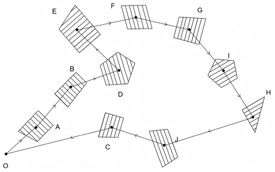
Figure 1.
An example of weeds distribution in a turf scene, where “O” is the starting point.
Without loss of generality, we define Problems 1 and 2 as follows:
Problem 1 (Efficient path planning). Determine the path of minimal cost that enables the UGV to traverse all weed subregions and fully cover each subregion while satisfying dynamic constraints. This problem can be decomposed into two steps: (1) Find a path achieving full coverage within each subregion; (2) Find the shortest path to access all subregions.
Problem 2 (Precise path following). The four-wheel differential drive UGV must precisely localize itself using GPS and orientation information, and accurately track the planned weeding path.
2.1.2. Traveling Salesman Problem and Genetic Algorithm
The Traveling Salesman Problem (TSP) aims to find the shortest path for a salesman starting from the origin, traversing each city exactly once, and finally returning to the origin [36,37,38]. The objective of TSP is to minimize the total distance that the salesman travels, i.e.,
where is the distance from city to and is a binary indicator of whether the salesman has passed from city to subject to the constraints that each city can only be visited once, and that only one city can be visited at a time.
The TSP presents significant computational complexity: as the number of cities increases, the number of possible route combinations increases exponentially, rendering the rapid identification of an optimal solution extremely difficult. To address this challenge, heuristic algorithms are typically employed to search for near-optimal solutions in the TSP, with Genetic Algorithms (GA) being a prime example. A genetic algorithm is an optimization algorithm inspired by biological evolutionary processes, simulating natural selection and genetic mechanisms to achieve optimization. This algorithm maintains a population of multiple individuals and employs genetic operations such as initialization, selection, crossover, and mutation to iteratively update the population toward the optimal solution. The specific process is shown in Algorithm 1: First, generate the initial population (Line 1); then, parent individuals are selected from the population (Line 6). This process evaluates each individual’s chromosome adaptability to the environment by defining a fitness function . Based on the calculated fitness values , a subset of chromosomes from the current population is selected as parents for the next generation. The higher the fitness of the chromosome, the greater the probability of being selected. Subsequently, a decision is made regarding whether to perform the crossover operation on the selected parent individuals (Lines 8–10). The mutation operation is carried out in lines 12–13, after which the generated offspring are added to the new population (Line 15). The mutation operation simulates the gene mutation in biological genetics, introduces new genes into the population, and prevents the algorithm from premature convergence. Finally, the optimal individual is identified from the population of the last generation (Line 20).
| Algorithm 1: Genetic Algorithm | |
| Input: | |
| Output: | |
| 1 | Initialization population: ⊳ Generate popSize |
| 2 | for do |
| 3 | |
| 4 | |
| 5 | while do |
| 6 | ⊳ |
| 7 | if then |
| 8 | ⊳ Generate offspring individuals |
| 9 | else |
| 10 | |
| 11 | end if |
| 12 | if then |
| 13 | ⊳ Perform mutation on the individual |
| 14 | end if |
| 15 | ⊳ |
| 16 | end while |
| 17 | ⊳ Update current population |
| 18 | |
| 19 | end for |
| 20 | |
2.1.3. Pure Pursuit
As shown in Figure 2, for a robot employing a two-wheel differential kinematic model, the robot’s angular velocity can be calculated from the speeds of the left and right wheels, as follows:
where is the turning radius, is the wheelbase, and , , are the linear velocities of the robot’s left wheel, centroid, and right wheel, respectively. Therefore, the inverse kinematics model can be obtained via
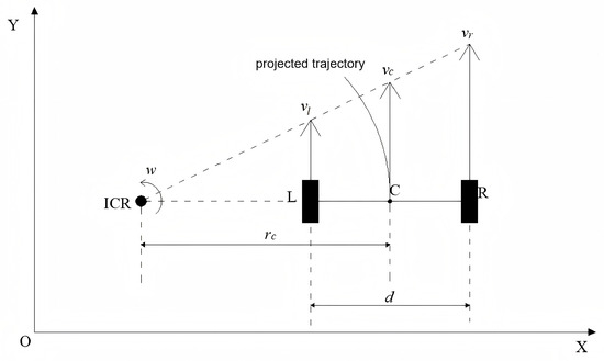
Figure 2.
Two-wheel differential kinematics model.
Equation (5) establishes the foundation for the path tracking algorithm. The core concept of the pure pursuit algorithm is to guide the vehicle along a path by calculating the curvature from its current position to a point on the predefined path (i.e., the target point or preview point), while controlling the robot through angular velocity calculations. The robot continuously tracks the next preview point from its current location until reaching the path’s endpoint. The pure pursuit algorithm first calculates the angle between the vehicle’s current heading and the line connecting the vehicle’s current position to the preview point. The current heading of the vehicle is obtained via
where is the center position of the rear axle of the vehicle, is the preview point position, is the heading angle of the vehicle, and returns the 2-argument arctangent value in angle measure. Then, the steering angle follows
where is the preview distance, i.e., the distance between the robot location and the point , and is the vehicle wheelbase.
2.2. Efficient Weeding Path Planning
2.2.1. Complete Coverage of a Single Sub-Region
The UGV first determines a path planning scheme for full coverage within a single subregion. This paper opts to construct a local coordinate system, which offers greater intuitiveness and conciseness compared to the translation baseline approach [39,40]. This approach is more intuitive and concise. Concurrently, a zigzag coverage strategy [41] is adopted, which enables the UGV to turn at the edges of subregions and thereby effectively avoids redundant coverage compared to the spiral method [42].
This paper proposes a practical solution for implementing the zigzag coverage path planning algorithm in the local coordinate system. Most weed subregions can be approximated as convex polygons, and convex polygons possess simple geometric properties with broad applications in the complete coverage problem [43]. Assuming that a subregion is a convex polygonal shape with vertices , , , , as shown in Figure 3. The equations of the boundary line between and in coordinate, noted as , is given by
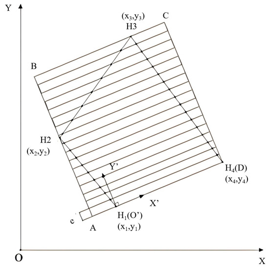
Figure 3.
Irregular area complete coverage path planning diagram, including boundary and trajectory points.
By choosing as the origin of a local coordinate , we construct a circumscribed rectangular region that shares with . Translating a distance of along direction times yields two intersection points with the edges of the weeding region, namely and , as revealed in Figure 3. With the changes of , the inflection points are formulated in two cases. In the cases of ,
where denotes the intersection between two lines and , and is the angle between and the -axis. In the cases of , Equation (9) becomes
By finding the two intersection points generated after each translation, a series of inflection points can be obtained to determine an efficient, complete coverage path for a single subregion.
2.2.2. Sequence Planning for Multiple Subregions
In turf maintenance, weed distribution typically manifests as multiple discrete small regions, requiring the turf weeding vehicle to cover multiple such subregions when performing the weeding task. Therefore, it is necessary to consider the sequence planning between each subregion, which can be modeled as the classic TSP, in which each weed subregion is regarded as a city to be traversed through.
Definition 1 (Representative Node). Once a complete coverage path for a single subregion is determined, it has a starting point and an ending point . However, and may be interchangeable. Furthermore, directly searching for the shortest path that traverses all subregions and of all subregions may result in incorrect connections between the starting and ending points of different weed subregions. The method for forming subregion representative nodes is illustrated in Figure 4. Additionally, the midpoint connecting point and point is adopted as the representative node for the subregion, which represents the location of each subregion.
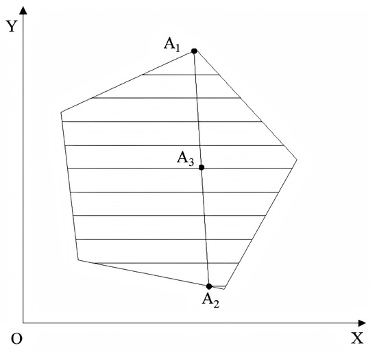
Figure 4.
A schematic diagram of a representative node.
To address the TSP and achieve rapid convergence with enhanced local search capabilities, this paper proposes an improved genetic algorithm. This algorithm achieves adaptive optimization by adjusting the crossover and mutation probability functions within genetic operations. The genetic algorithm employs chromosome encoding to represent the access sequences of subregions and iteratively optimizes the population through genetic operations such as initialization, selection, crossover, and mutation to seek the optimal solution for the TSP.
- (1)
- Population Initialization: In the genetic algorithm, the traversal order of subregions serves as the encoding, with path length defined as the objective function. Due to the use of integer encoding, each chromosome undergoes a validity check to ensure the absence of duplicate nodes. Subsequently, the population (i.e., the set of chromosomes) is initialized as the initial solution. The chromosome count is set to , where represents the number of subregions.
The stability and convergence of the genetic algorithm are influenced by the fitness function. In this paper, the sum of the distances is used as the fitness function to measure whether the solution is optimal, which is defined as
where denotes the gene (i.e., node), and denotes the shortest distance between two points. represents the inverse of the total distance. The smaller the total distance, the higher the fitness.
- (2)
- Selection: This paper employs a roulette wheel selection strategy to determine the probability of an individual being selected for the next generation in the genetic selection process. Assuming there are a total of individuals, with the fitness value of the individual denoted as , the probability of the individual being selected is given by
- (3)
- Crossover: The crossover probability is critical to algorithm performance. If its value is too low, the algorithm may become trapped in local optima. Conversely, if the value is too high, convergence slows, resulting in an increased number of iterations. To achieve a balanced solution, we propose an adaptive crossover probability function defined as follows:
When , individuals in the population exhibit relatively better fitness, making the algorithm prone to getting stuck in local optima. To prevent premature convergence, the crossover probability should be appropriately reduced to minimize genetic exchange between high-fitness individuals. Conversely, when , individuals in the population demonstrate poorer fitness. Increasing the crossover probability facilitates the combination of high-fitness individuals, accelerating algorithm convergence.
Regarding crossover strategies, this paper employs a sequential crossover method. This method involves randomly selecting sub-sequences from the parent generation and copying them to corresponding positions in the offspring. This ensures that the generated paths are non-repetitive and encompass all nodes.
- (4)
- Mutation: In traditional genetic algorithms, the performance of mutation operations largely depends on the setting of the mutation probability . However, is typically set quite low, which increases the likelihood of the algorithm becoming trapped in local optima. This paper proposes an adaptive mutation probability function that adjusts based on an individual’s fitness value: when an individual’s fitness is poor, the mutation probability is increased, and it is gradually decreased throughout the algorithm’s iterations, thereby enhancing optimization efficiency. The adaptive mutation probability function realizes the adaptive adjustment of by
2.3. Precise Path Following
2.3.1. Sensor Fusion for Improved Localization
When navigating undulating terrain, GPS positioning may experience delays. While RTK-GPS enables high-precision positioning, its lower update frequency and signal obstructions allow the IMU to utilize its high-frequency measurement data for dead reckoning. The fusion of GPS and IMU in navigation not only mitigates delays but also corrects drift issues arising from cumulative errors in inertial navigation systems [44,45]. Moreover, closed-loop control is employed to compare the desired trajectory with the actual position. By calculating and feeding back lateral deviations, precise trajectory tracking is achieved, as illustrated in Figure 5.
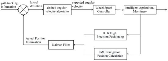
Figure 5.
Flow chart of navigation control algorithm.
When employing a direct loose-coupled RTK GPS/IMU integrated navigation solution, the GPS and IMU operate independently to provide navigation parameters tailored to environmental requirements. First, the UGV acquires raw data from both the GPS receiver and the IMU. The GPS provides position, velocity, and time information, while the IMU supplies inertial data such as acceleration and angular velocity. Subsequently, the vehicle preprocesses the raw data and employs a Kalman filter to fuse GPS and IMU data. Based on sensor characteristics and error models, the measurement results undergo fusion processing to obtain more precise navigation solutions.
Set the state variables of the KF to the coordinates , velocity , and attitude angles of the weeding robot in the geographic coordinate system at time k.
The motion equations of the weeding robot in the planar coordinate system are:
where t is the sampling period, h is the satellite antenna installation height, and represents the three-axis angular velocity in the vehicle coordinate system, which can serve as input to the KF.
Define the state equations and measurement equations required for filtering as:
where A and B are the state transition matrix, is the state vector at time k − 1, and are the state vector and system control input at time k, respectively, is the process disturbance noise, is the system observation matrix, and is the observation noise.
The prediction process is as follows:
where represents the state estimate at time k − 1, denotes the state prediction at time k − 1 for time k, is the posterior estimation error covariance matrix at time k − 1, is the estimation error covariance matrix from time k − 1 to time k, and Q is the process noise covariance matrix.
After obtaining the predicted values, state updates begin, yielding the gain coefficients. The Kalman filter has been implemented with automatic iterative updates to obtain real-time estimates of the system state.
2.3.2. Dynamic Pure Pursuit Algorithm for Accurate Path Following
After an UGV plans its weeding path and achieves precise positioning, it must travel accurately along that path. Upon receiving the current latitude/longitude and the waypoint coordinates via the Jetson development board, the heading angle and distance difference are converted into the linear velocity and angular velocity of the weeding robot. The left and right wheel speeds are then calculated using an inverse kinematics model. These values are transmitted to the STM32 microprocessor via the serial port and converted into PWM output.
As shown in Figure 6, with the robot’s current position as the origin and the target point coordinates as , the geometric relationships in the figure indicate that:
where is the preview distance, is the angular error between the current heading angle and the target heading angle, and is the lateral range of the motion radius.
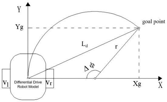
Figure 6.
Pure tracking model diagram.
Based on the relationship between angular velocity and linear velocity, the adjustment factor for angular velocity at a given linear velocity can be determined.
Substitute the real-time angular velocity obtained from the weeding robot into the inverse kinematics model of the differential robot to calculate the wheel speeds for the left and right wheels. Transmitting these values to the slave machine enables path tracking.
Unlike traditional pure pursuit algorithms, the relationship between preview distance and robot speed is no longer a simple linear function; instead, a quadratic function describes this relationship to mitigate measurement errors.
Since the faster the UGV moves, the larger the preview distance should be. Moreover, even when the robot is stationary, it maintains a minimal preview distance to enhance the system’s robustness. Thus, is defined as
where is the robot velocity, is the base of the preview distance, which is set to 2 m in this paper. and are correlation coefficients between the preview distance and the speed.
Set the drive wheelbase to 1 m, the time interval to 0.1 s, and the initial coordinates to (0, 0). Then, build a pure pursuit model for a two-wheel differential robot using Python in PyCharm 2019.2.6. Input the real-time angular velocity obtained from the weeding robot into the two-wheel differential motion model to calculate the rotational speeds of the left and right wheels. Send these speeds to the slave machine to achieve path tracking. Through a series of simulation experiments, parameters , , and were fitted. Figure 7 displays the simulation results for small trajectory deviations, with preview distances set at 2 m and 4 m, and corresponding ground vehicle speeds of 2 m/s and 4 m/s, respectively. The red curve represents the actual trajectory, while the black curve denotes the predefined trajectory. Therefore, the formula for calculating the preview distance given in this paper is:
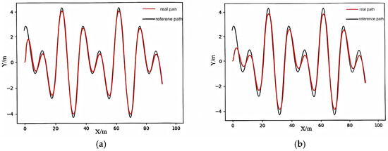
Figure 7.
Trajectory diagrams of the improved pure pursuit algorithm under two scenarios: (a) Preview distance of 4 m at a speed of 2 m/s. (b) Preview distance of 8 m at a speed of 4 m/s.
The improved pure pursuit algorithm significantly enhances the tracking process for low-speed turf weeding robots, resulting in greater efficiency, stability, and a more streamlined operation.
3. Results
3.1. Simulation Results for Path Planning
To conduct the simulation experiment, ten sets of latitude and longitude coordinates were selected from the Nanjing Forestry University playground. An environmental map was constructed to obtain the corresponding two-dimensional plane coordinates A, B, C, D, E, F, G, H, I, and J after Gaussian projection [46]. These coordinates are shown in Figure 8 and Table 1.
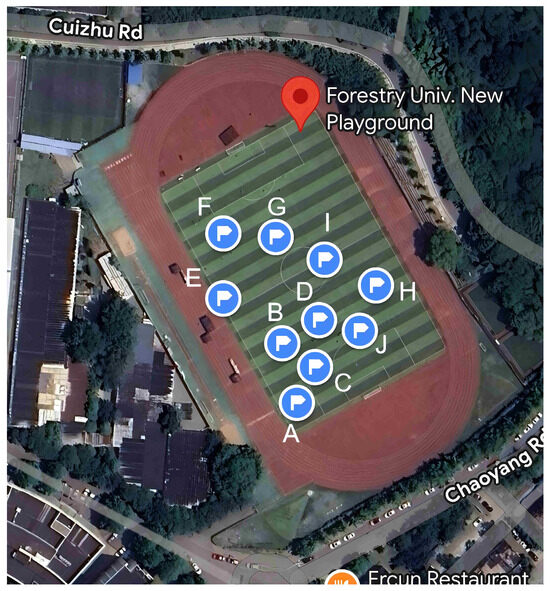
Figure 8.
Coordinates sampled from the playground of Nanjing Forestry University.

Table 1.
Latitude and longitude coordinates and Gaussian plane coordinates.
To address Problem 1, an adaptive design of the crossover probability and mutation functions was implemented in the genetic algorithm to compute the shortest path that traverses each node.
Path planning experiments were conducted on a laptop with an Intel Core i5-1240P processor (12 cores/16 threads, max 4.4 GHz) and 16 GB RAM. The genetic algorithm was implemented in Python 3.7. With 10 node coordinates as input, to ensure sufficient convergence and align with TSP parameter selection recommendations, the population size was set to 200 and the maximum iteration count to 200. The base crossover probability was set to 0.85 and the base mutation probability to 0.03 to promote population optimization while avoiding population homogeneity. The evolutionary process is illustrated in Figure 9, the planned path and the time required for genetic manipulation are shown in Figure 10. After 48 iterations of the genetic algorithm, the shortest path traversing all nodes was obtained in approximately 0.1958 s. This path spans 232.18 m, with the corresponding traversal sequence being A → B → D → E → F → G → I → H → J → C.
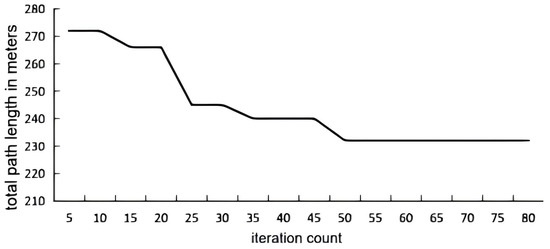
Figure 9.
Evolutionary process of genetic algorithm.
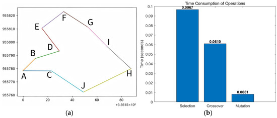
Figure 10.
Planned path and iteration time for genetic operations. (a) Shortest path map. (b) Iteration time required for each genetic operation.
In addition to path planning experiments in real-world scenarios, we selected two turf scenarios of different scales for path planning simulations using data from the TSPLIB dataset. The two scenarios are: one covering approximately 30,000 square meters with 10 subregion nodes, and another covering approximately 90,000 square meters with 30 subregion nodes. We employed the K-nearest neighbor (KNN) algorithm, a random algorithm (RA), and the improved genetic algorithm designed in this paper to solve these problems, analyzing the performance of the three algorithms. For each turf scenario, 10 repeated experiments were conducted using three distinct algorithms. The results are presented in Table 2, while the shortest paths are illustrated in Figure 11.
Table 2.
Path length and execution time under three algorithms.
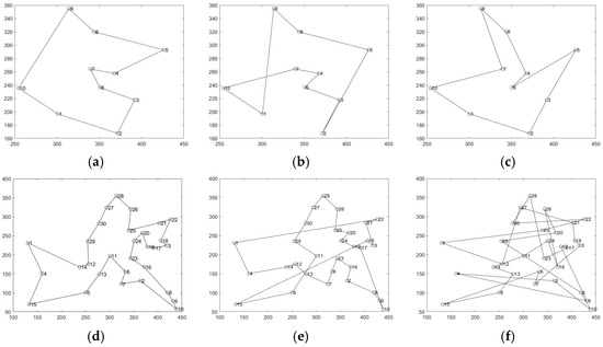
Figure 11.
The shortest path planning diagram for three algorithms in two scenarios. (a) Small-scale scenario genetic algorithm. (b) Small-scale scenario nearest neighbor algorithm. (c) Small-scale scenario random algorithm. (d) Large-scale scenario genetic algorithm. (e) Large-scale scenario nearest neighbor algorithm. (f) Large-scale scenario random algorithm.
3.2. Experimental Results for Path Following
3.2.1. Hardware Development
In order to verify the performance of sensor fusion and the dynamic pure pursuit algorithm, we developed a weeding robot platform to carry out field tests. Figure 12 illustrates the overall structure of the weeding robot (1.2 m × 1 m × 0.75 m). It features a four-wheel differential drive configuration, with the front two wheels serving as drive wheels and the rear two wheels functioning as caster wheels. The system employs an 86-step motor (3404HS60U14, HamDerBurg, Shenzhen, China) paired with a PF90-016P2MB gear reducer (Xingweida Automation Technology Co., Ltd., Dongguan, Guangdong, China) and a Handebao digital two-phase stepper driver (Dezhi High-tech Co., Ltd., Shenzhen, China). Powered by a 48 V battery, it effectively drives the weeding robot’s movement even under heavy loads. The control device is fixed above the weeding setter mobile platform for controlling the motors. The RTK positioning system employs the UM980 as the base station board and the UM982 as the rover station board. The inertial sensor utilizes the HWT9052 nine-axis strapdown IMU.
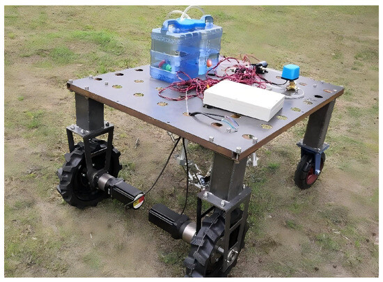
Figure 12.
Prototype of the weeding robot.
The platform utilizes a Jetson development board (Jetson Xavier NX, NVIDIA Corporation, Santa Clara, CA, USA, with 8 GB of memory and a maximum computing power of 21 TOPS) as the processor for its embedded Linux system. It efficiently reads IMU data via the Inter-Integrated Circuit (IIC) communication interface, accurately capturing key robotic attitude parameters including roll angle, pitch angle, and yaw angle. Additionally, the board connects to the RTK-GPS module using USB-to-serial technology, receiving latitude and longitude data that complies with the NMEA0183 standard to track the robot’s location in real time.
The Jetson development board reads pre-stored waypoint data (the results of path planning) and compares it with the position data filtered by the Kalman filter. This process precisely calculates the distance deviation and heading deviation between the robot’s current location and the next target waypoint.
Based on these calculations, the Jetson sends specific robotic control commands (angular velocity and linear velocity data) to the STM32 microprocessor, which outputs PWM pulses to the stepper motors. Set the pulse duty cycle to 0.5, and adjust the stepper motor’s rotational speed by modifying the pulse frequency. These motors control the weeding robot’s movement, steering, and braking functions, ultimately enabling autonomous navigation for the turf weeding.
3.2.2. Sensor Fusion
Positioning data fusion can be achieved on the Jetson development board using KF. To validate changes in latitude and longitude measurements before and after Kalman filtering, this paper developed two sets of dynamic and static measurement procedures. The test site was selected as the new playground at Nanjing Forestry University. Static measurements involved multiple measurements at fixed locations and intervals, plotting trajectory diagrams before and after latitude–longitude filtering. Additionally, to validate the system’s dynamic performance, data were collected both before and after filtering while the system was in motion. Trajectories for static measurements before and after filtering are shown in Figure 13a,b, while those for dynamic measurements are illustrated in Figure 13c.
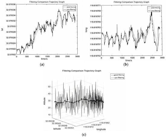
Figure 13.
Trajectory diagrams for latitude and longitude measurements: (a) Static latitude measurement. (b) Static longitude measurement. (c) Dynamic latitude and longitude measurement.
The KF significantly optimizes trajectory smoothness: First, it effectively suppresses high-frequency noise. Frequency domain analysis indicates a noise suppression ratio (NSR) of 3.5:1, eliminating over 70% of noise and effectively filtering out irregular interference in sensor measurements. Second, it substantially reduces trajectory fluctuations. The standard deviation (SD) of velocity in the latitude and longitude directions decreased from 0.3 m/s and 0.4 m/s before filtering to 0.1 m/s and 0.15 m/s, respectively, achieving approximately 60% improvement in smoothness.
3.2.3. Dynamic Pure Pursuit
This paper improves the pure pursuit algorithm by selecting one based on dynamically adjusting the preview distance. To verify the stability of the improved pure pursuit algorithm and its suitability for weeding operations under varying weed densities, experiments compared the lateral deviation in the robot’s travel speed at different speeds. With the sampling interval set to 1 s, the lateral deviations obtained at robot speeds of 0.6, 0.8, and 1.0 m/s are shown in Figure 14a–c, respectively.
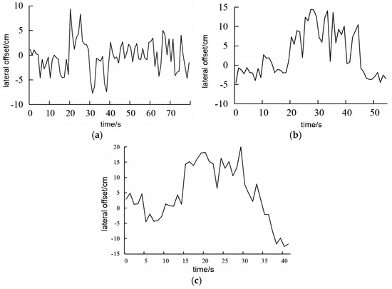
Figure 14.
Lateral deviation at three speeds of the weeding robot: (a) 0.6 m/s. (b) 0.8 m/s. (c) 1.0 m/s.
The test results are summarized in Table 3. When the traveling speed of the applicator robot is 0.6, 0.8 and , the number of acquisitions is 79, 54 and 41 times, and the root mean square error is 0.36, 0.81 and , respectively. The coefficient of variation (CV) for these speeds was 9.3%, 10.96%, and 13.66%, with valid data proportions of 98.7%, 98.1%, and 97.6%.
Table 3.
Comparison of navigation test errors at three different speeds.
4. Discussion
In this study, the path planning method based on the TSP achieved a tenfold reduction in path length compared to the baseline translation-based full-coverage approach. Furthermore, after the adaptive design of the genetic algorithm, although computational time increased slightly compared to the nearest-neighbor and random algorithms, the planned paths were the shortest and showed no instances of path crossing. In small-region turf scenarios (≤10 nodes), the improved genetic algorithm demonstrated limited effects on path shortening. However, for large-region turfs (≥30 nodes), it produced significantly more efficient paths.
Due to inherent sensor noise and environmental electromagnetic interference, the latitude–longitude curve deviated from static characteristics before applying the KF, exhibiting high-frequency oscillations and spike fluctuations in accuracy. Kalman filtering significantly enhances fusion positioning performance, successfully eliminating 70% of the original noise. Trajectory fluctuations are substantially reduced, with smoothness improved by approximately 60%, markedly enhancing the stability of the positioning system. The dispersion of measurement data was significantly reduced. Particularly during dynamic measurements, the dispersion of height readings exhibited a marked tendency toward stability. When the robot travels at speeds between 0.6 and 1.0 m/s, tracking accuracy reaches centimeter-level precision, with the coefficient of variation in deviation controlled within 15%, demonstrating strong tracking stability. As the vehicle speed increased, the lateral deviation progressively increased. Adjust the travel speed based on turf weed density, adapting to varying weed density environments with different speed settings to enhance the automation level of precision weed control equipment.
This paper proposes a path planning solution for scenarios involving large turf areas with multiple weed zones and well-defined boundaries. Previous path planning studies have focused on row-cropped fields, and research on agricultural multi-objective path planning has primarily emphasized collision avoidance [47], which does not perfectly suit expansive turfs. This paper integrates scheduling path planning and full-coverage path planning, enabling more flexible and efficient paths for weeding robots. Turf surfaces lack distinct topographical features, making machine vision-based navigation research challenging for turf applications. SLAM navigation technology is better suited for indoor scenarios such as greenhouses. This paper’s GPS/IMU integrated navigation approach fully leverages the open terrain advantage of outdoor turf while simplifying the complexity of navigation algorithms. While it has partially improved the weeding efficiency of robotic mowers, certain limitations remain. The experiments were conducted based on known information about weed-infested areas within the turf. Future research could explore deep learning-based weed recognition to enhance the robot’s intelligence. Meanwhile, the path planning algorithm employed in the experiment exhibits slightly longer computation times. Future research will focus on developing faster-converging scheduling path planning algorithms.
5. Conclusions
We propose an autonomous navigation solution for wheeled unmanned ground vehicles, designed to optimize path planning and precisely execute turf weeding paths. For randomly distributed multi-region turf weed environments, we specifically introduce a path planning algorithm based on the TSP.
By constructing a two-dimensional environmental map, we employ a genetic algorithm to adaptively design the crossover probability function and mutation probability function within genetic operations, addressing the interval scheduling problem in multi-weed regions. Subsequently, coordinate points are determined through boundary baseline translation to achieve comprehensive path planning across subregions.
Concurrently, RTK GPS/IMU integrated navigation, combined with an improved pure pursuit algorithm, further enhances path tracking accuracy. Simulation and hardware experiments validate this autonomous navigation strategy, yielding encouraging results.
Author Contributions
Conceptualization and methodology, X.L. and Y.C.; validation, X.L.; formal analysis and investigation, L.Y. and X.L.; resources and data curation, Y.C.; writing—original draft preparation, L.Y. and X.L.; writing—review and editing, J.C. and L.Y.; visualization, X.L.; supervision, project administration, and funding acquisition, J.C. and Y.C. All authors have read and agreed to the published version of the manuscript.
Funding
This work was funded by the National Natural Science Foundation of China under Grant No. 32072498, the Natural Science Research Project of Jiangsu Higher Education Institutions under Grant 24KJD510007, the Research Start Fund of Nanjing Normal University under Grant 184080H201B60, and the Undergraduate Innovation Training Program Project of Jiangsu under Grant 202310298014Z.
Data Availability Statement
The original contributions presented in this study are included in the article. Further inquiries can be directed to the corresponding authors.
Conflicts of Interest
The authors declare no conflicts of interest.
Abbreviations
The following abbreviations are used in this manuscript:
| TSP | Traveling Salesman Problem |
| RTK | Real-Time Kinematic |
| GPS | Global Positioning System |
| RRT | Rapidly Exploring Random Trees |
| APF | Artificial Potential Field |
| IMU | Inertial Measurement Unit |
| KF | Kalman filter |
| PID | Proportional-Integral-Derivative |
| UGV | Unmanned Ground Vehicle |
| GA | Genetic Algorithm |
| IIC | Inter-Integrated Circuit |
| PWM | Pulse Width Modulation |
| NSR | Noise Suppression Ratio |
| SD | Standard Deviation |
| CV | Coefficient of Variation |
| KNN | K-Nearest Neighbor |
| RA | Random Algorithm |
References
- Jin, X.; Bagavathiannan, M.; McCullough, P.E.; Chen, Y.; Yu, J. A deep learning-based method for classification, detection, and localization of weeds in turfgrass. Pest Manag. Sci. 2022, 78, 4809–4821. [Google Scholar] [CrossRef]
- Bakhshipour, A.; Jafari, A. Evaluation of support vector machine and artificial neural networks in weed detection using shape features. Comput. Electron. Agric. 2018, 145, 153–160. [Google Scholar] [CrossRef]
- Jin, X.; Zhao, H.; Kong, X.; Han, K.; Lei, J.; Zu, Q.; Chen, Y.; Yu, J. Deep learning-based weed detection for precision herbicide application in turf. Pest Manag. Sci. 2025, 81, 3597–3609. [Google Scholar] [CrossRef]
- Yu, J.; Sharpe, S.M.; Schumann, A.W.; Boyd, N.S. Deep learning for image-based weed detection in turfgrass. Eur. J. Agron. 2019, 104, 78–84. [Google Scholar] [CrossRef]
- Jin, X.; McCullough, P.E.; Liu, T.; Yang, D.; Zhu, W.; Chen, Y.; Yu, J. A smart sprayer for weed control in bermudagrass turf based on the herbicide weed control spectrum. Crop Prot. 2023, 170, 106270. [Google Scholar] [CrossRef]
- Shi, J.; Bai, Y.; Diao, Z.; Zhou, J.; Yao, X.; Zhang, B. Row detection BASED navigation and guidance for agricultural robots and autonomous vehicles in row-crop fields: Methods and applications. Agronomy 2023, 13, 1780. [Google Scholar] [CrossRef]
- McElroy, J.S.; Strickland, M.; Nunes, L.R.T.; Magni, S.; Fontani, M.; Fontanelli, M.; Volterrani, M. Robotic mowing technology in turfgrass management: Past, present, and future. Crop Sci. 2025, 65, e70081. [Google Scholar] [CrossRef]
- Hasan, A.M.; Sohel, F.; Diepeveen, D.; Laga, H.; Jones, M.G. A survey of deep learning techniques for weed detection from images. Comput. Electron. Agric. 2021, 184, 106067. [Google Scholar] [CrossRef]
- Jin, X.; Han, K.; Zhao, H.; Wang, Y.; Chen, Y.; Yu, J. Detection and coverage estimation of purple nutsedge in turf with image classification neural networks. Pest. Manag. Sci. 2024, 80, 3504–3515. [Google Scholar] [CrossRef] [PubMed]
- Su, W.-H.; Slaughter, D.C.; Fennimore, S.A. Non-destructive evaluation of photostability of crop signaling compounds and dose effects on celery vigor for precision plant identification using computer vision. Comput. Electron. Agric. 2020, 168, 105155. [Google Scholar] [CrossRef]
- Shi, Y.; Li, Q.; Bu, S.; Yang, J.; Zhu, L. Research on Intelligent Vehicle Path Planning Based on Rapidly-Exploring Random Tree. Math. Probl. Eng. 2020, 2020, 5910503. [Google Scholar] [CrossRef]
- Wang, X.; Luo, X.; Han, B.; Chen, Y.; Liang, G.; Zheng, K. Collision-free path planning method for robots based on an improved rapidly-exploring random tree algorithm. Appl. Sci. 2020, 10, 1381. [Google Scholar] [CrossRef]
- Fu, B.; Chen, L.; Zhou, Y.; Zheng, D.; Wei, Z.; Dai, J.; Pan, H. An improved A* algorithm for the industrial robot path planning with high success rate and short length. Robot. Auton. Syst. 2018, 106, 26–37. [Google Scholar] [CrossRef]
- Jeon, C.-W.; Kim, H.-J.; Yun, C.; Gang, M.; Han, X. An entry-exit path planner for an autonomous tractor in a paddy field. Comput. Electron. Agric. 2021, 191, 106548. [Google Scholar] [CrossRef]
- Fan, X.; Guo, Y.; Liu, H.; Wei, B.; Lyu, W. Improved artificial potential field method applied for AUV path planning. Math. Probl. Eng. 2020, 2020, 6523158. [Google Scholar] [CrossRef]
- Yao, Q.; Zheng, Z.; Qi, L.; Yuan, H.; Guo, X.; Zhao, M.; Liu, Z.; Yang, T. Path planning method with improved artificial potential field—A reinforcement learning perspective. IEEE Access 2020, 8, 135513–135523. [Google Scholar] [CrossRef]
- Galceran, E.; Carreras, M. A survey on coverage path planning for robotics. Robot. Auton. Syst. 2013, 61, 1258–1276. [Google Scholar] [CrossRef]
- Huang, X.; Sun, M.; Zhou, H.; Liu, S. A multi-robot coverage path planning algorithm for the environment with multiple land cover types. IEEE Access 2020, 8, 198101–198117. [Google Scholar] [CrossRef]
- Wu, C.; Dai, C.; Gong, X.; Liu, Y.J.; Wang, J.; Gu, X.D.; Wang, C.C. Energy-efficient coverage path planning for general terrain surfaces. IEEE Robot. Autom. Lett. 2019, 4, 2584–2591. [Google Scholar] [CrossRef]
- Lakshmanan, A.K.; Mohan, R.E.; Ramalingam, B.; Le, A.V.; Veerajagadeshwar, P.; Tiwari, K.; Ilyas, M. Complete coverage path planning using reinforcement learning for tetromino based cleaning and maintenance robot. Autom. Constr. 2020, 112, 103078. [Google Scholar] [CrossRef]
- Yang, L.W.; Li, P.; Wang, T.; Miao, J.C.; Tian, J.Y.; Chen, C.Y.; Tan, J.; Wang, Z.J. Multi-area collision-free path planning and efficient task scheduling optimization for autonomous agricultural robots. Sci. Rep. 2024, 14, 18347. [Google Scholar] [CrossRef]
- Ji, J.; Zhao, J.-S.; Misyurin, S.Y.; Martins, D. Precision-Driven Multi-Target Path Planning and Fine Position Error Estimation on a Dual-Movement-Mode Mobile Robot Using a Three-Parameter Error Model. Sensors 2023, 23, 517. [Google Scholar] [CrossRef]
- Liu, K.; Yu, J.; Huang, Z.; Liu, L.; Shi, Y. Autonomous navigation system for greenhouse tomato picking robots based on laser SLAM. Alex. Eng. J. 2024, 100, 208–219. [Google Scholar] [CrossRef]
- Simon, J. Fuzzy Control of Self-Balancing, Two-Wheel-Driven, SLAM-Based, Unmanned System for Agriculture 4.0 Applications. Machines 2023, 11, 467. [Google Scholar] [CrossRef]
- Nagasaka, Y.; Saito, H.; Tamaki, K.; Seki, M.; Kobayashi, K.; Taniwaki, K. An autonomous rice transplanter guided by global positioning system and inertial measurement unit. J. Field Robot. 2009, 26, 537–548. [Google Scholar] [CrossRef]
- Vieira, D.; Orjuela, R.; Spisser, M.; Basset, M. Positioning and attitude determination for precision agriculture robots based on IMU and two RTK GPSs sensor fusion. IFAC-Pap. 2022, 55, 60–65. [Google Scholar] [CrossRef]
- Yan, Y.; Zhang, B.; Zhou, J.; Zhang, Y.; Liu, X.a. Real-time localization and mapping utilizing multi-sensor fusion and visual–IMU–wheel odometry for agricultural robots in unstructured, dynamic and GPS-denied greenhouse environments. Agronomy 2022, 12, 1740. [Google Scholar] [CrossRef]
- Li, S.; Zhang, M.; Ji, Y.; Zhang, Z.; Cao, R.; Chen, B.; Li, H.; Yin, Y. Agricultural machinery GNSS/IMU-integrated navigation based on fuzzy adaptive finite impulse response Kalman filtering algorithm. Comput. Electron. Agric. 2021, 191, 106524. [Google Scholar] [CrossRef]
- Farag, W. Complex trajectory tracking using PID control for autonomous driving. Int. J. Intell. Transp. 2020, 18, 356–366. [Google Scholar] [CrossRef]
- Moshayedi, A.J.; Abbasi, A.; Liao, L.; Li, S. Path planning and trajectroy tracking of a mobile robot using bio-inspired optimization algorithms and PID control. In Proceedings of the 2019 IEEE International Conference on Computational Intelligence and Virtual Environments for Measurement Systems and Applications (CIVEMSA), Tianjin, China, 14–16 June 2019. [Google Scholar] [CrossRef]
- Qun, R. Intelligent control technology of agricultural greenhouse operation robot based on fuzzy PID path tracking algorithm. INMATEH-Agric. Eng. 2020, 62, 181–190. [Google Scholar] [CrossRef]
- Li, Q.; Xu, Y.; Bu, S.; Yang, J. Smart vehicle path planning based on modified PRM algorithm. Sensors 2022, 22, 6581. [Google Scholar] [CrossRef]
- Samuel, M.; Hussein, M.; Mohamad, M.B. A review of some pure-pursuit based path tracking techniques for control of autonomous vehicle. Int. J. Comput. Appl. 2016, 135, 35–38. [Google Scholar] [CrossRef]
- Xu, X.; Wang, K.; Li, Q.; Yang, J. An Optimal Hierarchical Control Strategy for 4WS-4WD Vehicles Using Nonlinear Model Predictive Control. Machines 2024, 12, 84. [Google Scholar] [CrossRef]
- Yang, Y.; Li, Y.; Wen, X.; Zhang, G.; Ma, Q.; Cheng, S.; Qi, J.; Xu, L.; Chen, L. An optimal goal point determination algorithm for automatic navigation of agricultural machinery: Improving the tracking accuracy of the Pure Pursuit algorithm. Comput. Electron. Agric. 2022, 194, 106760. [Google Scholar] [CrossRef]
- Haldurai, L.; Madhubala, T.; Rajalakshmi, R. A study on genetic algorithm and its applications. Int. J. Comput. Sci. Eng. 2016, 4, 139–143. [Google Scholar]
- Lambora, A.; Gupta, K.; Chopra, K. Genetic algorithm-A literature review. In Proceedings of the 2019 International Conference on Machine Learning, Big Data, Cloud and Parallel Computing (COMITCon), Faridabad, India, 14–16 February 2019; pp. 380–384. [Google Scholar] [CrossRef]
- Mirjalili, S. Evolutionary algorithms and neural networks. Stud. Comput. Intell. 2019, 780, 43–53. [Google Scholar] [CrossRef]
- Li, J.; Sheng, H.; Zhang, J.; Zhang, H. Coverage path planning method for agricultural spraying UAV in arbitrary polygon area. Aerospace 2023, 10, 755. [Google Scholar] [CrossRef]
- Pour Arab, D.; Spisser, M.; Essert, C. Complete coverage path planning for wheeled agricultural robots. J. Field Robot. 2023, 40, 1460–1503. [Google Scholar] [CrossRef]
- Zhu, L.; Yao, S.; Li, B.; Song, A.; Jia, Y.; Mitani, J. A geometric folding pattern for robot coverage path planning. In Proceedings of the 2021 IEEE International Conference on Robotics and Automation (ICRA), Xi’an, China, 30 May–5 June 2021. [Google Scholar] [CrossRef]
- Wang, N.; Yang, X.; Wang, T.; Xiao, J.; Zhang, M.; Wang, H.; Li, H. Collaborative path planning and task allocation for multiple agricultural machines. Comput. Electron. Agric. 2023, 213, 108218. [Google Scholar] [CrossRef]
- Höffmann, M.; Patel, S.; Büskens, C. Optimal guidance track generation for precision agriculture: A review of coverage path planning techniques. J. Field Robot. 2024, 41, 823–844. [Google Scholar] [CrossRef]
- Guang, X.; Gao, Y.; Liu, P.; Li, G. IMU data and GPS position information direct fusion based on LSTM. Sensors 2021, 21, 2500. [Google Scholar] [CrossRef] [PubMed]
- Ryu, J.H.; Gankhuyag, G.; Chong, K.T. Navigation system heading and position accuracy improvement through GPS and INS data fusion. J. Sens. 2016, 2016, 7942963. [Google Scholar] [CrossRef]
- Mataija, M.; Pogarčić, M.; Pogarčić, I. Helmert transformation of reference coordinating systems for geodesic purposes in local frames. Procedia Eng. 2014, 69, 168–176. [Google Scholar] [CrossRef][Green Version]
- Chakraborty, S.; Elangovan, D.; Govindarajan, P.L.; ELnaggar, M.F.; Alrashed, M.M.; Kamel, S. A comprehensive review of path planning for agricultural ground robots. Sustainability 2022, 14, 9156. [Google Scholar] [CrossRef]


Disclaimer/Publisher’s Note: The statements, opinions and data contained in all publications are solely those of the individual author(s) and contributor(s) and not of MDPI and/or the editor(s). MDPI and/or the editor(s) disclaim responsibility for any injury to people or property resulting from any ideas, methods, instructions or products referred to in the content. |
© 2025 by the authors. Licensee MDPI, Basel, Switzerland. This article is an open access article distributed under the terms and conditions of the Creative Commons Attribution (CC BY) license (https://creativecommons.org/licenses/by/4.0/).