Article

Evaluating Time-Series Prediction of Temperature, Relative Humidity, and CO2 in the Greenhouse with Transformer-Based and RNN-Based Models

1
Department of Integrative Biological Sciences and Industry, Sejong University, Seoul 05006, Republic of Korea
2
Digilog Inc., Seoul 05006, Republic of Korea
3
Smart Farm Research Center, Korea Institute of Science and Technology (KIST), Gangneung 25451, Republic of Korea
*
Author to whom correspondence should be addressed.
Agronomy 2024, 14(3), 417; https://doi.org/10.3390/agronomy14030417
Submission received: 22 November 2023 / Revised: 26 January 2024 / Accepted: 16 February 2024 / Published: 21 February 2024
(This article belongs to the Special Issue The Applications of Deep Learning in Smart Agriculture)

Abstract

:
In greenhouses, plant growth is directly influenced by internal environmental conditions, and therefore requires continuous management and proper environmental control. Inadequate environmental conditions make plants vulnerable to pests and diseases, lower yields, and cause impaired growth and development. Previous studies have explored the combination of greenhouse actuator control history with internal and external environmental data to enhance prediction accuracy, using deep learning-based models such as RNNs and LSTMs. In recent years, transformer-based models and RNN-based models have shown good performance in various domains. However, their applications for time-series forecasting in a greenhouse environment remain unexplored. Therefore, the objective of this study was to evaluate the prediction performance of temperature, relative humidity (RH), and CO2 concentration in a greenhouse after 1 and 3 h, using a transformer-based model (Autoformer), variants of two RNN models (LSTM and SegRNN), and a simple linear model (DLinear). The performance of these four models was compared to assess whether the latest state-of-the-art (SOTA) models, Autoformer and SegRNN, are as effective as DLinear and LSTM in predicting greenhouse environments. The analysis was based on four external climate data samples, three internal data samples, and six actuator data samples. Overall, DLinear and SegRNN consistently outperformed Autoformer and LSTM. Both DLinear and SegRNN performed well in general, but were not as strong in predicting CO2 concentration. SegRNN outperformed DLinear in CO2 predictions, while showing similar performance in temperature and RH prediction. The results of this study do not provide a definitive conclusion that transformer-based models, such as Autoformer, are inferior to linear-based models like DLinear or certain RNN-based models like SegRNN in predicting time series for greenhouse environments.

1. Introduction

Plant growth in greenhouses is greatly influenced by internal environmental conditions, and therefore requires continuous management and proper environmental control. Inadequate environmental conditions make plants vulnerable to pests and diseases, result in decreased yields, and cause impaired growth and development [1,2,3]. To ensure optimal growing conditions, monitoring is critical to predict changes in the greenhouse environment. However, environmental factors in the greenhouse exhibit complex and non-linear dynamics, making prediction a particularly challenging task. As a result, simple models and formulas are often insufficient to accurately predict environmental changes [4,5].
In previous studies, researchers have primarily used the internal and external environmental data of the greenhouse to predict the conditions inside, or they have combined the data with the control history of the actuators in the greenhouse. As an example of the use of only greenhouse environmental data to predict indoor conditions, Moon et al. [6] utilized nine environmental parameters that were recorded at 10 min intervals to predict changes in the carbon dioxide (CO2) concentration, using an artificial neural network (ANN) model. These authors reported high accuracy even in the absence of ventilation data, demonstrating the potential of a neural network-based model for predicting CO2 in greenhouses. Subsequently, Moon et al. [7] used an LSTM model to predict the CO2 concentration and achieved promising accuracy despite the rapid and inconsistent fluctuations in CO2 levels in the greenhouse. As an alternative to neural network-based approaches, Cao et al. [8] implemented a tree-based machine learning model combined with time-series features. Their proposed model demonstrated high predictive performance even though the model was simple and fast to train, in contrast with deep learning-based models such as RNNs and LSTMs.
Recent studies have attempted to predict greenhouse conditions by integrating internal and external environmental data, as well as data from actuator control history. Choi et al. [9] used a combination of environmental data and operating values of control devices to predict the temperature and relative humidity in a greenhouse 10–120 min in advance. Jung et al. [10] conducted a comparative analysis of RNN-LSTM-based models and NARX models and obtained satisfactory forecasts for temperature and CO2 concentration. However, the models did not perform as well in predicting relative humidity in the greenhouse, particularly under unusual outdoor weather conditions such as heavy rainfall and storms. Ullah et al. [11] attempted to predict three greenhouse environmental factors: temperature, CO2 concentration, and relative humidity. To improve the prediction accuracy, they proposed an ANN-based model using a refined Kalman filter and reported high accuracy even with noisy sensor readings in the greenhouse. Cai et al. [12] utilized a light gradient boosting machine learning (LightGBM) model. They reported that LightGBM was applicable not only to the prediction of the greenhouse environment but also to real-time predictive control applications. Jung et al. [13] used an LSTM model to predict two crucial factors related to moisture in greenhouses: relative humidity and evapotranspiration. Their study validated the feasibility of applying data-driven deep learning models and demonstrated that the model was able to predict greenhouse conditions in real-world applications, assuming a consistent and extensive collection of sufficient environmental data.
Overall, the above-mentioned studies have shown that incorporating the greenhouse actuator control history with indoor and outdoor environmental data tends to achieve enhanced prediction performance. Various approaches ranging from machine learning models to neural network-based deep learning models have been investigated, and most of them have demonstrated satisfactory performance in the context of the given experiment. However, to the best of our knowledge, there are no reports using transformer-based models for time-series prediction in greenhouse environments, despite their superior performance over conventional deep learning models in many applications across various domains.
In recent years, the transformer has demonstrated exceptional performance in many fields, including natural language processing [14], speech recognition [15], and computer vision [16]. Consequently, many transformer-based models have been proposed, and the performance of these models has been continuously enhanced [17,18]. Research on transformer-based models is also gaining popularity in the field of time-series forecasting [19]. Along with this trend, the comparative advantage of transformer-based models over non-transformer-based models has become a primary focus of investigation [20,21,22]. Nonetheless, transformer-based models have not yet been explored to address time-series forecasting in a greenhouse environment.
In addition, recent research indicated that the SegRNN model, an enhanced version of the conventional RNN model for time-series prediction, has achieved remarkable performance. The conventional RNN often suffers from performance degradation due to excessively long look-back windows and forecast horizons. The SegRNN model counters this by integrating segment-wise iterations and parallel multi-step forecasting, which greatly reduces the number of RNN iterations required. These changes have led to significant improvements in both prediction accuracy and inference speed. However, just like transformer-based models, the SegRNN model has not yet been tested for time-series prediction in greenhouse environments.
Therefore, the objective of this study was to evaluate the predictive performance of temperature, relative humidity (RH), and CO2 concentration in a greenhouse after 1 and 3 h, using a transformer-based model (Autoformer) [23], variants of two RNN models (LSTM [24] and SegRNN [25]), and a simple linear model (DLinear) [21]. The performance of these four models was compared to assess whether the transformer-based model (Autoformer) and RNN-based model (SegRNN) are as effective as the linear-based model in predicting greenhouse environments. The models were trained and tested using inputs from greenhouse climate conditions and the status of the greenhouse actuators, collected over the previous three days. Prediction performance was evaluated with four metrics: the mean absolute error (MAE), mean squared error (MSE), root-mean-squared error (RMSE), and coefficient of determination (R2).

2. Materials and Methods

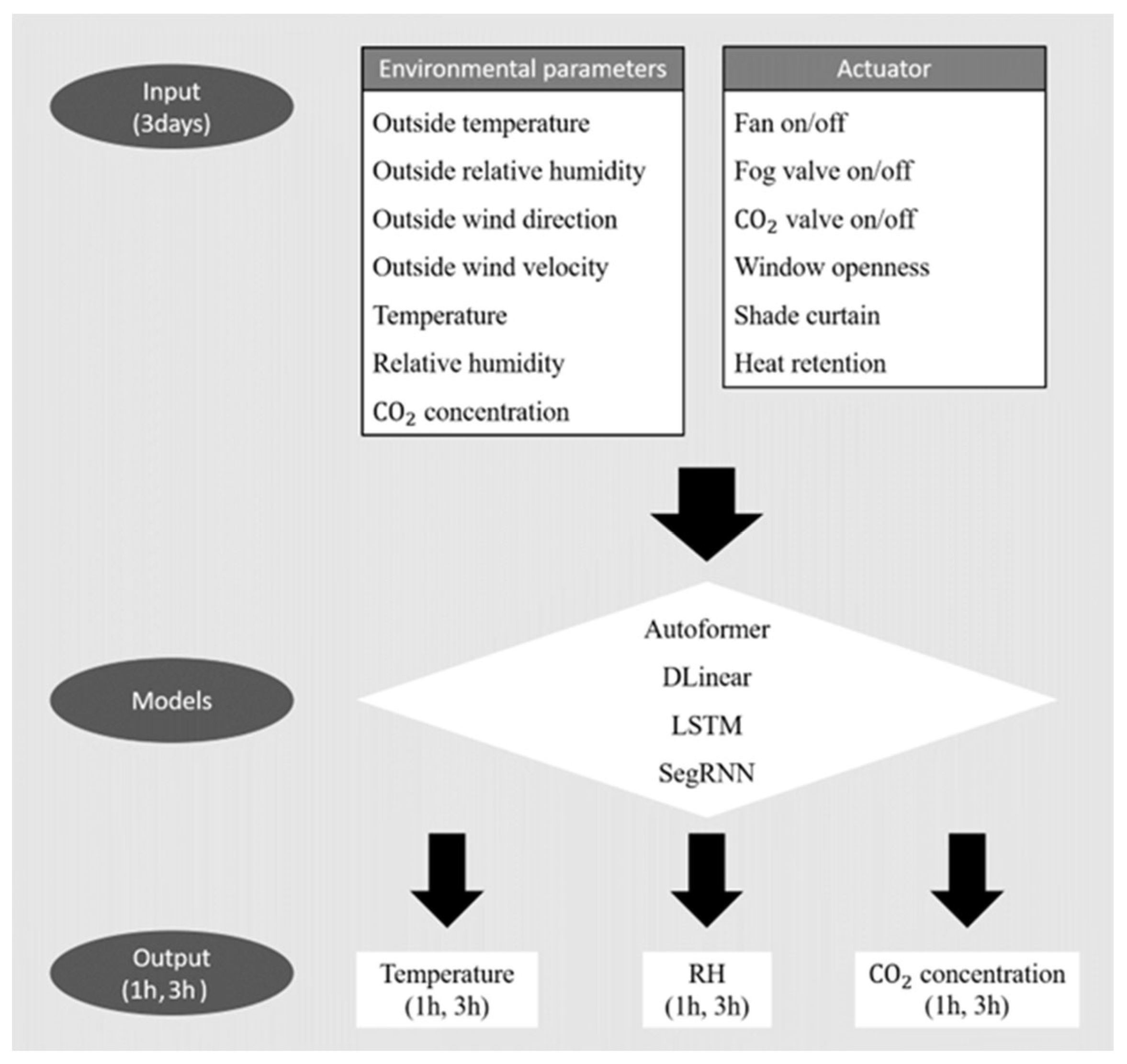
2.1. Data Acquisition and Preprocessing

The dataset for this study was obtained from a Venlo-type tomato greenhouse operated by the Korea Institute of Science and Technology (KIST) in Gangneung, Gangwon-do, Republic of Korea, with coordinates 37.79868 N, 128.85617 E (Figure 1). An internal sensor module (SH-VT260, Soha Tech, Seoul, Republic of Korea) for measuring temperature, humidity, and CO2 inside the greenhouse was installed in height-adjustable positions according to the height of the tomato plants. In addition, an external weather station (Vantage Pro2, Davis Instruments, Hayward, CA, USA) was installed 2 m above the roof of the greenhouse. From 22 September 2020 to 29 June 2021, data were collected on an hourly basis from an internal sensor module as well as from an external weather station, and included the status of various greenhouse actuators. This resulted in a total of 6744 records being included in the dataset.
For model training, a set of 13 sensor and actuator values was used (Table 1): four measurements from an external weather station (temperature, relative humidity, wind direction, and wind speed), three measurements from an internal sensor module (temperature, relative humidity, and CO2 concentration), and the statuses of six actuators (circulating fan, fogging valve, CO2 injection valve, window opening ratio, shading curtain opening ratio, and heat retention curtain opening ratio). The range of each value is shown in Table 2.
Collected data were preprocessed to handle missing values and outliers. In the raw dataset, missing values accounted for 0.38% of the internal environmental variables and 0.69% of the external environmental variables and actuators. Missing values were interpolated from the previous and subsequent observations, under the assumption that there were no substantial changes in the values within an hour. Outliers were identified as values 1.5 times higher or lower than the interquartile range of the 25th and 75th percentiles of the raw data distribution and were then removed. After preprocessing, the dataset was divided into train, validation, and test sets in a ratio of 7:1:2, respectively.

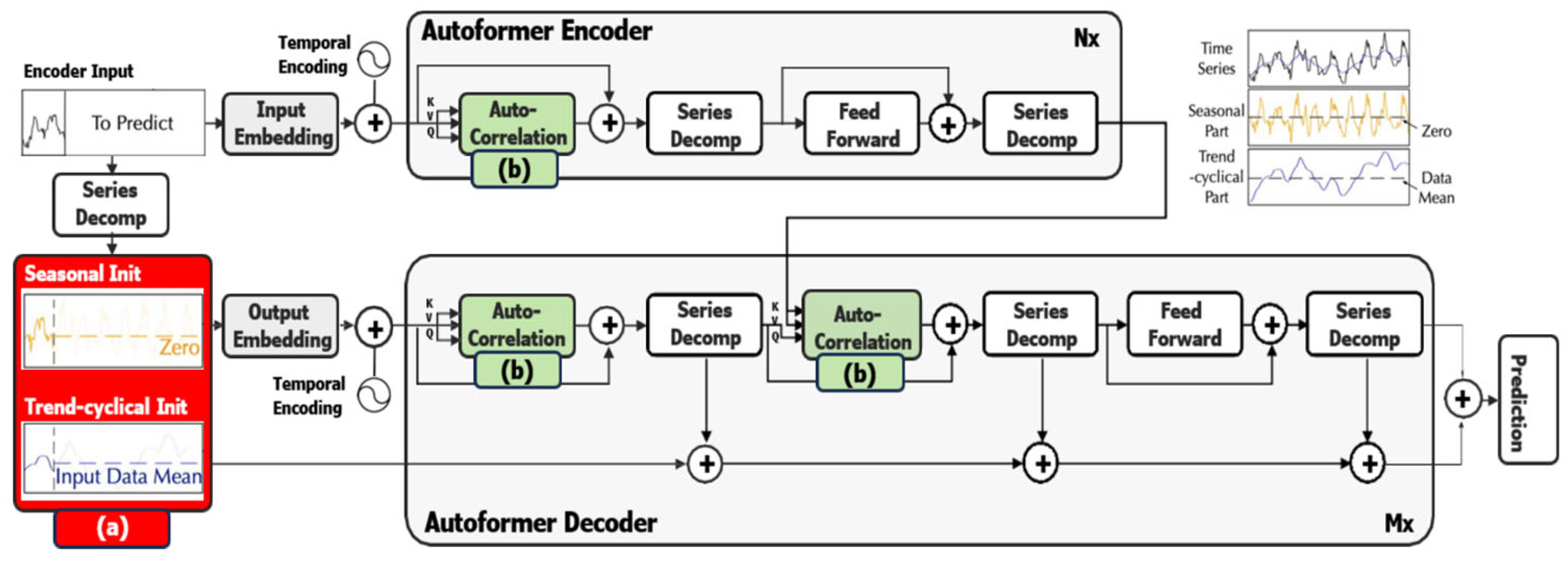
2.2. Transformer-Based Model: Autoformer

Over the past few years, transformers have demonstrated outstanding performance in a wide range of applications, such as natural language processing (NLP) and computer vision (CV) [14,15,16]. In NLP, the GPT and BERT models are representative transformer-based models that have received considerable attention in recent years [17,26]. In CV, transformer-based models have been increasingly applied and shown to outperform conventional convolutional neural networks (CNNs) in classification, detection, and segmentation tasks [27,28,29].
Researchers have recently applied transformers to time-series forecasting. Unlike RNNs, which rely on recurrent mechanisms, or CNNs, which use convolutions, the transformer is based purely on an attention mechanism. This mechanism allows it to capture long-range dependencies more effectively than RNN-based models, and thus provides an advantage in predicting time series [30]. However, the transformer’s self-attention makes it difficult to efficiently handle long sequences of input and output, which is a drawback for time-series prediction.
To address these issues, Autoformer was proposed [23]. Designed to improve prediction performance, Autoformer incorporates features specific to time-series data. It discriminates between seasonals and trends (series decomposition) before feeding the time-series data to the decoder (Figure 2a), allowing in-depth learning of complex temporal patterns during training. In addition, Autoformer uses an auto-correlation mechanism to overcome the inefficiencies of the self-attention in existing transformers (Figure 2b). As a result, Autoformer has demonstrated better prediction performance compared to current state-of-the-art (SOTA) models [23]. In particular, for weather forecasting such as outdoor temperature and humidity, which show a similar pattern to greenhouse time-series data, Autoformer outperformed the previous SOTA model, LSTM, by 21% in terms of MSE.

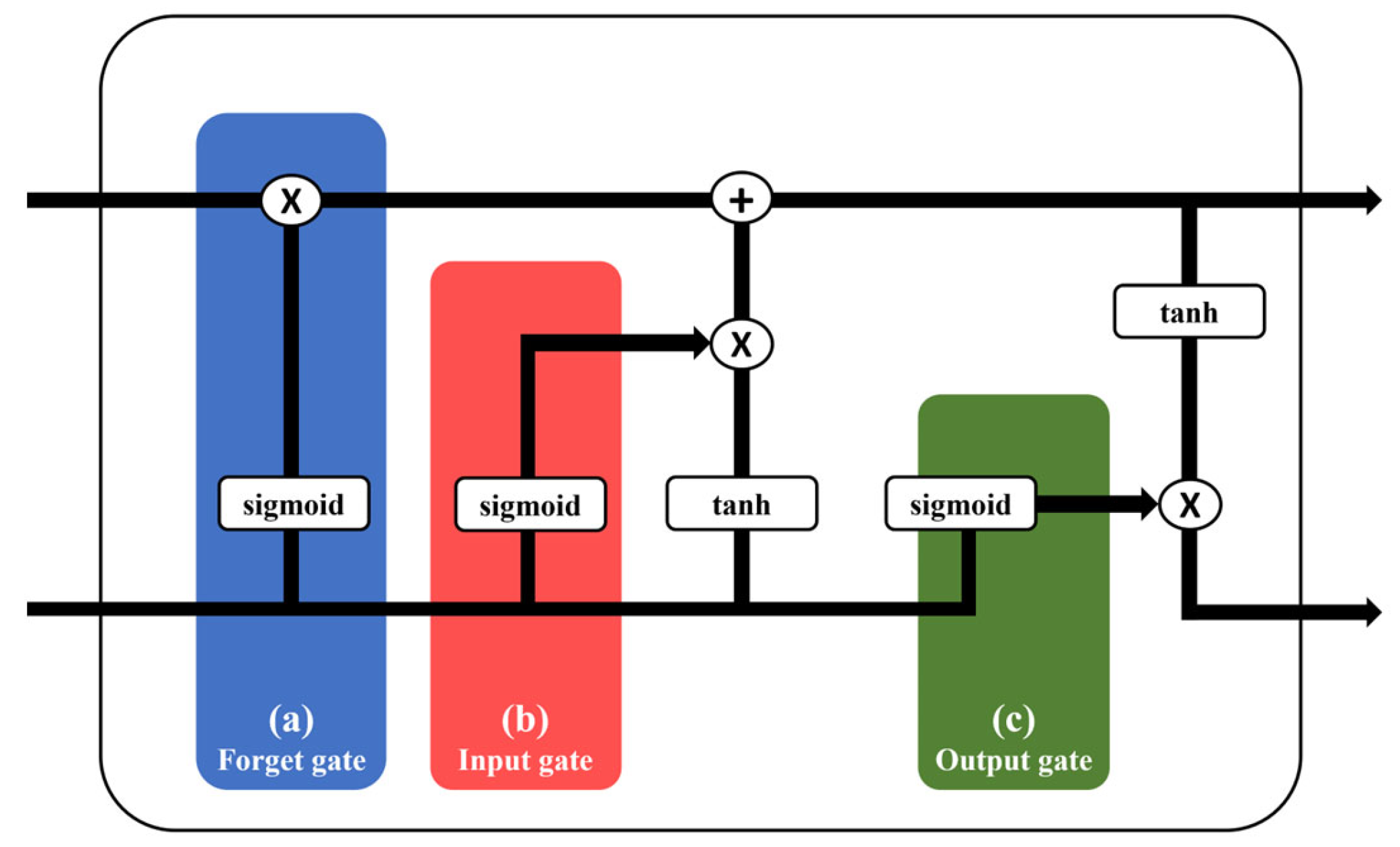
2.3. RNN-Based Model: (1) Long Short-Term Memory (LSTM)

RNN-based models have been widely used in time-series forecasting, mainly due to their ability to incorporate sequential data flows in making predictions [31,32,33,34,35]. In particular, LSTM is designed to solve the vanishing and exploding gradient problems of conventional RNNs, which is advantageous for addressing long-term memory loss. Accordingly, numerous studies have demonstrated the effectiveness of LSTM for time-series prediction [10,13,24,36,37,38,39,40,41,42,43]. LSTM consists of a forget gate (Figure 3a), an input gate (Figure 3b), and a sigmoid output gate (Figure 3c). Hochreiter and Schmidhuber [24] provide a detailed description of their computations. In this study, LSTM was used as a baseline, along with DLinear, to evaluate the performance of Autoformer and SegRNN.

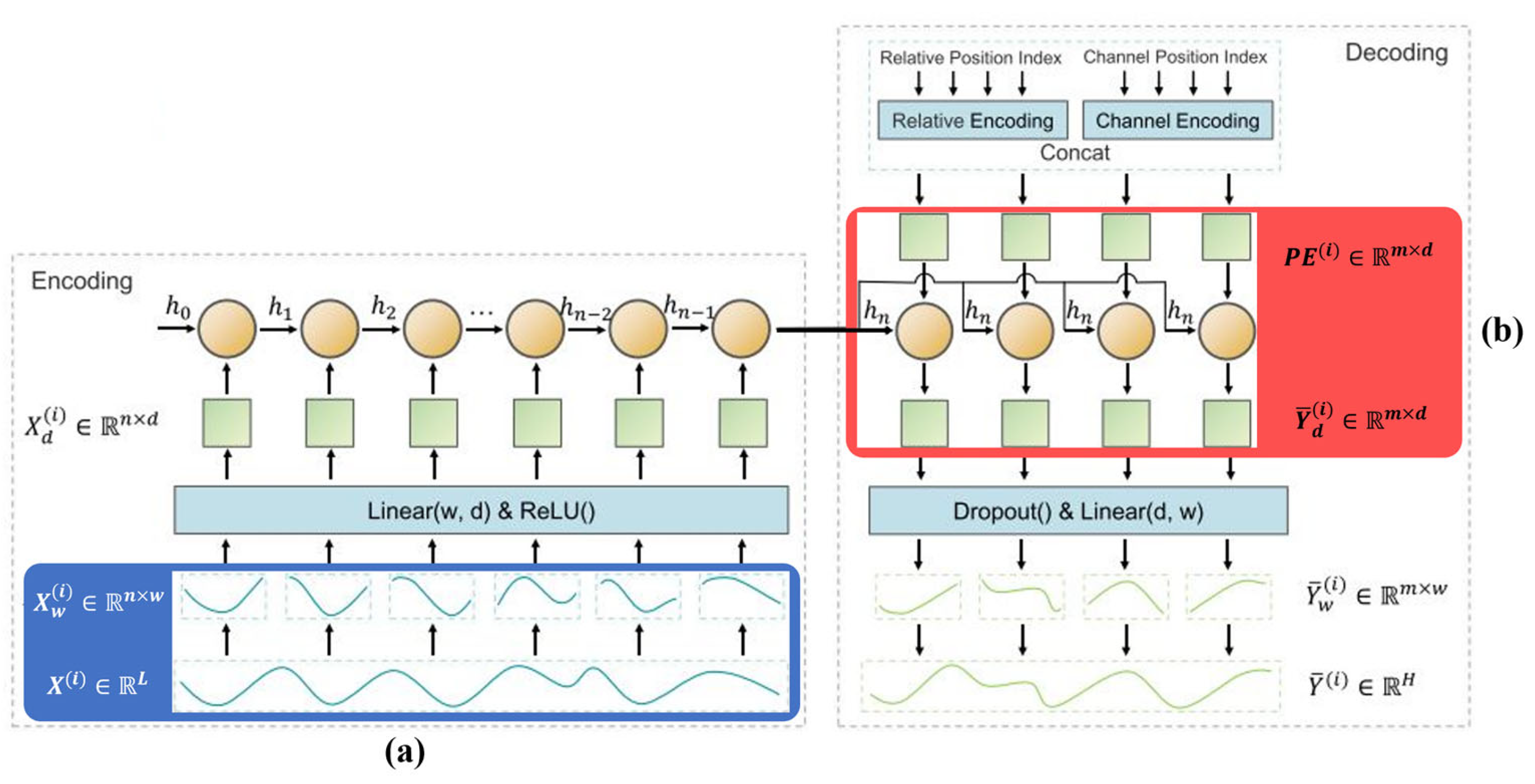
2.4. RNN-Based Model: (2) Segment RNN (SegRNN)

Despite their widespread use, RNN-based models have fallen behind transformer-based models in terms of their prediction performance for time-series data. However, recent research has revealed that SegRNN, an improved version of the conventional RNN, achieves remarkable performance in time-series prediction [25]. Conventional RNNs typically face performance issues due to excessively long look-back windows and forecast horizons. SegRNN addresses this by reducing the number of iterations through segment-wise iteration (Figure 4a) and parallel multistep forecasting (Figure 4b), which can enhance the prediction performance for time series.

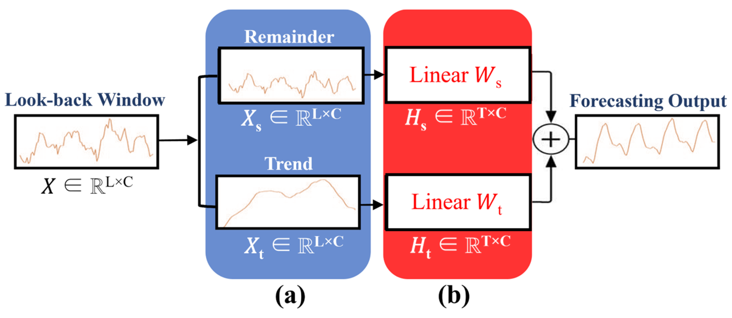
2.5. Linear-Based Model: DLinear

DLinear is proposed to preserve the fundamental properties of time-series data while avoiding the complexity associated with the transformer. Similar to Autoformer, DLinear uses a time-series decomposition approach, and its structure is straightforward: (1) it splits the input time series into trend and remainder components (Figure 5a), and (2) it applies a single-layer linear network (Figure 5b). The formula for this procedure is outlined in Equations (1)–(3).
Internally, DLinear operates as a linear model where the weights corresponding to the seasonality and trend of the time series are multiplied by its decomposition inputs (Equations (2) and (3)). This approach allows an intuitive interpretation by analyzing the weights. In addition, the single-layer linear network reduces computational time, memory usage, and the number of parameters compared to transformer-based models, and thus efficiently performs without the need for hyperparameter tuning [21]. Recent studies have suggested that this approach can predict time series better than transformer-based models [45,46].
X ^ = H s + H t
H s = W s X s T × C   ( remainder component )
H t = W t X t T × C   ( trend component )
where X ^ is the prediction values, W s T × L and W t T × L are two linear layers, T is the future timesteps, and L is the history timesteps, as shown in Figure 3.

2.6. Impliementation Details and Model Evaluation

The models were trained using the Adam optimizer with an initial learning rate of 5 × 10 3 . Model training was performed with 100 epochs and 16 batch sizes. The default value of the Gaussian Error Linear Unit (GELU) was set to the activation function.
Model performance was evaluated using four metrics, MAE (mean absolute error), MSE (mean squared error), RMSE (root-mean-squared error), and R2 (R-squared coefficient of determination), as shown in Equations (4)–(7):
MAE = i = 1 n y i y i ^ n
MSE = 1 n i = 1 n y i y i ^ 2
RMSE = 1 n i = 1 n y i y i ^ 2
R 2 = 1 i = 1 n y i y i ^ 2 i = 1 n y i y i ¯ 2
where n is the number of values, y i are the observed values, y i ^ are the predicted values, and y i ¯ is the mean value of the observed outputs.
An overview of the experiments conducted in this study is presented in Figure 6.

3. Results

Four models (Autoformer, DLinear, LSTM, and SegRNN) were compared to evaluate prediction performance for greenhouse conditions using three days of time-series data as input. Overall, a simple linear model, DLinear, consistently outperformed the others in most of the metrics for the prediction after 1 h and 3 h. The RNN-based model, SegRNN, showed an almost similar, but slightly lower, performance than DLinear.
Table 3 shows the predictions of the temperature, RH, and CO2 concentration inside the greenhouse after 1 h. The R2 values of DLinear were considerably high with values of 0.938, 0.857, and 0.783 for temperature, RH, and CO2, respectively. SegRNN also showed a similar performance, but slightly lower compared to DLinear. In terms of CO2 concentration, SegRNN had the highest R2 value of 0.875, which was 11.7% better than that of DLinear and 203% better than that of LSTM.
In contrast, both the transformer-based model, Autoformer, and another RNN-based model, LSTM, showed poor performance. The R2 values for Autoformer were 0.744, 0.636, and 0.590 for temperature, RH, and CO2, respectively. For LSTM, these values were 0.645, 0.404, and 0.289, respectively. In each case, these values were considerably lower than those achieved by DLinear and SegRNN.
Table 4 shows the predictions of the temperature, RH, and CO2 concentration inside the greenhouse after 3 h. Again, the R2 values of DLinear were relatively high with values of 0.833, 0.680, and 0.580 for temperature, RH, and CO2, respectively. SegRNN also showed a similar performance, but slightly lower compared to DLinear. In terms of CO2 concentration, SegRNN had the highest R2 value of 0.711, which was 22% better than that of DLinear and 299% better than that of LSTM.
In contrast, both the transformer-based model, Autoformer, and another RNN-based model, LSTM, showed worse performance. The R2 values for Autoformer were 0.554, 0.411, and 0.488 for temperature, RH, and CO2, respectively. For LSTM, these values were 0.447, 0.253, and 0.178, respectively. In each case, these values were considerably lower than those achieved by DLinear and SegRNN.
This strong performance of DLinear and SegRNN supports their effectiveness in processing complex greenhouse time-series data and illustrates their suitability for predicting greenhouse conditions. However, there was a large decrease in the accuracy of both models for the 3 h predictions compared to 1 h predictions. The largest decrease in performance, as indicated by the R2 values, was observed for the DLinear CO2 prediction, where the 3 h prediction decreased by 26% compared to the 1 h. Despite an 18% decrease, from 0.875 to 0.711 in R2 values, SegRNN’s CO2 prediction maintained the highest performance of all models for both 1 h and 3 h.
Figure 7 and Figure 8 show a detailed comparison of actual and predicted values by Autoformer, DLinear, LSTM, and SegRNN. A visual analysis of these plots suggests that DLinear and SegRNN generally displayed better prediction performance compared to the other models. For temperature, both DLinear and SegRNN showed reasonable prediction. For RH, LSTM showed a prediction curve that was considerably different from the other three models and had the worst performance of all. In terms of CO2 concentration, SegRNN appeared to display the best performance, closely matching the actual values.

4. Discussion

This study evaluates the performance of four models—Autoformer, DLinear, LSTM, and SegRNN—in predicting time-series data for greenhouse environments. Although transformer-based models are known to perform very well in various domains, our results indicate that a simpler model, DLinear, and an RNN-based model, SegRNN, perform better in time-series prediction for greenhouses, compared to LSTM and Autoformer. This finding is in line with other recent studies that have suggested that transformer-based models may not be as effective in capturing the sequential characteristics of time-series data [21,44]. Indeed, DLinear has demonstrated strong predictive performance, especially when the time-series data have a clear trend and periodicity [20]. Moreover, DLinear’s capability to capture short- and long-range temporal relationships in time-series data, combined with its lower computational costs due to reduced memory and parameter requirements compared to transformer-based models, could potentially make it a viable baseline model for greenhouse environment prediction. In addition, SegRNN, which is designed to overcome the limitations of conventional RNNs for time-series prediction, demonstrated superior performance to LSTM, which is known for its robust performance in numerous studies. Since only very few studies have evaluated the effectiveness of SegRNNs in predicting greenhouse environmental time series, the result of this study is expected to have important implications in this field. Nevertheless, further studies are needed to validate these findings.
The results of this study do not provide a definitive conclusion that transformer-based models and RNN-based models, LSTM in particular, are inferior to linear-based models in predicting time series for greenhouse environments. In general, transformer-based models require extensive data for training [20]. However, the dataset used in this study was collected from only a single growing season. With a more comprehensive set of data collected over multiple growing seasons, the transformer-based model may perform better. The observed poor predictive performance of the transformer-based model in this study is likely due to incorrect trend prediction and over-fitting to sudden changes in the training data, which may have led to the performance degradation [47]. Therefore, there is potential to improve the performance of transformer-based models with larger and more diverse greenhouse time-series datasets. In support of this, a recent study showed that an improved variant of the transformer model outperformed DLinear in time-series prediction on larger datasets [30]. Research is still underway to improve the prediction of time series by developing a specialized structure of transformer variants that are focused on application scenarios and data types.
The results of this study are similar to or slightly worse than those of previous studies regarding the prediction of changes in a greenhouse environment. This may be due to the comparatively shorter data collection period in this study compared to those of other studies [9]. Nevertheless, our results with DLinear and SegRNN models were satisfactory in predicting temperature and RH changes after 1 and 3 h. SegRNN was particularly effective in predicting CO2 concentrations. CO2 concentrations in greenhouses are generally difficult to predict as their concentrations fluctuate rapidly and are also influenced by the complex interactions of various environmental factors within the greenhouse [7]. Factors such as photosynthetic activity, ventilation, and external weather conditions can all affect CO2 concentration, which makes them more challenging to predict than other environmental variables. Indeed, during the experimental greenhouse cultivation in this study, CO2 control had to be manually adjusted for a period of time due to external market factors. Temporary CO2 supply shortages and sudden price increases had occasionally led to restrictions on its use in the real world. Such issues pose a significant challenge to predictive models and suggest the need for a more sophisticated approach. Despite these conditions, SegRNN performed relatively well at predicting CO2 concentrations. Future research could focus on making these prediction models more robust to the factors mentioned above. This could be achieved by including additional external variables that have a direct or indirect impact on CO2 consumption. The investigation of advanced machine learning approaches for dealing with high-frequency data fluctuations in time series could also possibly improve the accuracy of predicting CO2 concentrations in greenhouse environments [48].
The implementation of time-series prediction models in greenhouse management can potentially provide significant environmental and economic benefits [49]. First, integrating these models with real-time control data allows for dynamic greenhouse management that enables a rapid response to changing environmental conditions, thereby improving crop yields. More accurate predictions of environmental conditions also allow for the more efficient use of resources such as water and energy, thereby reducing waste and minimizing environmental impact. Economically, such an approach can help reduce greenhouse operating costs and increase profitability.
Finally, the applicability of our results to other types of greenhouses remains uncertain because this research focused on a Venlo-type greenhouse. Therefore, future studies need to include environmental datasets acquired from different types of greenhouses. Expanding the dataset could potentially help develop more accurate models.

5. Conclusions

This study evaluated the prediction performance of temperature, relative humidity (RH), and CO2 concentration in a greenhouse environment using a transformer-based model (Autoformer), variants of two RNN models (LSTM and SegRNN), and a simple linear model (DLinear). Overall, DLinear and SegRNN consistently outperformed Autoformer and LSTM. Both DLinear and SegRNN performed well in general but were not as strong in predicting CO2 concentration. SegRNN outperformed DLinear in CO2 predictions while showing similar performance in temperature and RH prediction. The results of this study do not provide a definitive conclusion that transformer-based models, such as Autoformer, are inferior to linear-based models like DLinear or certain RNN-based models like SegRNN in predicting time series for greenhouse environments.

Author Contributions

Conceptualization, J.Y.A. and H.K.S.; data curation, S.H.P.; methodology, J.Y.A. and H.K.S.; software, J.Y.A. and H.P.; visualization, Y.K. and H.P.; formal analysis, S.H.P.; writing—original draft preparation, J.Y.A. and H.K.S.; writing—review and editing, H.K.S.; supervision, H.K.S.; funding acquisition, S.H.P. and H.K.S. All authors have read and agreed to the published version of the manuscript.

Funding

This work was supported by the Korea Institute of Planning and Evaluation for Technology in Food, Agriculture and Forestry (IPET) and the Korea Smart Farm R&D Foundation (KosFarm) through the Smart Farm Innovation Technology Development Program, funded by the Ministry of Agriculture, Food and Rural Affairs (MAFRA) and the Ministry of Science and ICT (MSIT), Rural Development Administration (RDA) (421026-04).

Data Availability Statement

Dataset available on request from the authors.

Acknowledgments

This study builds upon Ju Yeon Ahn’s MSc thesis [44] by introducing the following three key distinctions: (1) This study used a different dataset collected in a different greenhouse and at a different time. The dataset in this study was collected over one year in an experimental greenhouse at KIST, Korea; (2) This study goes further by incorporating the actuator control history in addition to the environmental variables to enrich the model inputs; (3) This study introduced a new model, SegRNN, along with new metrics for evaluating performance. To comprehensively assess the performance of the models, this study employed four evaluation metrics: MAE, MSE, RMSE, and R2.

Conflicts of Interest

Authors Ju Yeon Ahn and Hyun Kwon Suh were employed by the company Digilog Inc., Seoul, Republic of Korea. The remaining authors declare that the research was conducted in the absence of any commercial or financial relationships that could be construed as a potential conflict of interest.

References

  1. Grange, R.I.; Hand, D.W. A Review of the Effects of Atmospheric Humidity on the Growth of Horticultural Crops. J. Hortic. Sci. 1987, 62, 125–134. [Google Scholar] [CrossRef]
  2. Van Der Ploeg, A.; Heuvelink, E. Influence of Sub-Optimal Temperature on Tomato Growth and Yield: A Review. J. Hortic. Sci. Biotechnol. 2005, 80, 652–659. [Google Scholar] [CrossRef]
  3. Ohtaka, K.; Yoshida, A.; Kakei, Y.; Fukui, K.; Kojima, M.; Takebayashi, Y.; Yano, K.; Imanishi, S.; Sakakibara, H. Difference between Day and Night Temperatures Affects Stem Elongation in Tomato (Solanum lycopersicum) Seedlings via Regulation of Gibberellin and Auxin Synthesis. Front. Plant Sci. 2020, 11, 1947. [Google Scholar] [CrossRef] [PubMed]
  4. Fitz-Rodríguez, E.; Kubota, C.; Giacomelli, G.A.; Tignor, M.E.; Wilson, S.B.; McMahon, M. Dynamic Modeling and Simulation of Greenhouse Environments under Several Scenarios: A Web-Based Application. Comput. Electron. Agric. 2010, 70, 105–116. [Google Scholar] [CrossRef]
  5. Kamilaris, A.; Kartakoullis, A.; Prenafeta-Boldú, F.X. A Review on the Practice of Big Data Analysis in Agriculture. Comput. Electron. Agric. 2017, 143, 23–37. [Google Scholar] [CrossRef]
  6. Moon, T.W.; Jung, D.H.; Chang, S.H.; Son, J.E. Estimation of Greenhouse CO2 Concentration via an Artificial Neural Network That Uses Environmental Factors. Hortic. Environ. Biotechnol. 2018, 59, 45–50. [Google Scholar] [CrossRef]
  7. Moon, T.; Choi, H.Y.; Jung, D.H.; Chang, S.H.; Son, J.E. Prediction of CO2 Concentration via Long Short-Term Memory Using Environmental Factors in Greenhouses. Korean J. Hortic. Sci. Technol. 2020, 38, 201–209. [Google Scholar] [CrossRef]
  8. Cao, Q.; Wu, Y.; Yang, J.; Yin, J. Greenhouse Temperature Prediction Based on Time-Series Features and LightGBM. Appl. Sci. 2023, 13, 1610. [Google Scholar] [CrossRef]
  9. Choi, H.; Moon, T.; Jung, D.H.; Son, J.E. Prediction of Air Temperature and Relative Humidity in Greenhouse via a Multilayer Perceptron Using Environmental Factors. J. Bio-Environ. Control 2019, 28, 95–103. [Google Scholar] [CrossRef]
  10. Jung, D.H.; Kim, H.S.; Jhin, C.; Kim, H.J.; Park, S.H. Time-Serial Analysis of Deep Neural Network Models for Prediction of Climatic Conditions inside a Greenhouse. Comput. Electron. Agric. 2020, 173, 105402. [Google Scholar] [CrossRef]
  11. Ullah, I.; Fayaz, M.; Naveed, N.; Kim, D. ANN Based Learning to Kalman Filter Algorithm for Indoor Environment Prediction in Smart Greenhouse. IEEE Access 2020, 8, 159371–159388. [Google Scholar] [CrossRef]
  12. Cai, W.; Wei, R.; Xu, L.; Ding, X. A Method for Modelling Greenhouse Temperature Using Gradient Boost Decision Tree. Inf. Process. Agric. 2022, 9, 343–354. [Google Scholar] [CrossRef]
  13. Jung, D.-H.; Lee, T.S.; Kim, K.; Park, S.H. A Deep Learning Model to Predict Evapotranspiration and Relative Humidity for Moisture Control in Tomato Greenhouses. Agronomy 2022, 12, 2169. [Google Scholar] [CrossRef]
  14. Wolf, T.; Debut, L.; Sanh, V.; Chaumond, J.; Delangue, C.; Moi, A.; Cistac, P.; Rault, T.; Louf, R.; Funtowicz, M.; et al. Transformers: State-of-the-Art Natural Language Processing. In Proceedings of the 2020 Conference on Empirical Methods in Natural Language Processing: System Demonstrations, Online, 16–20 November 2020; pp. 38–45. [Google Scholar] [CrossRef]
  15. Dong, L.; Xu, S.; Xu, B. Speech-Transformer: A No-Recurrence Sequence-to-Sequence Model for Speech Recognition. In Proceedings of the 2018 IEEE International Conference on Acoustics, Speech and Signal Processing (ICASSP), Calgary, AB, Canada, 15–20 April 2018; pp. 5884–5888. [Google Scholar] [CrossRef]
  16. Khan, S.; Naseer, M.; Hayat, M.; Zamir, S.W.; Khan, F.S.; Shah, M. Transformers in Vision: A Survey. ACM Comput. Surv. (CSUR) 2022, 54, 1–41. [Google Scholar] [CrossRef]
  17. Han, X.; Zhang, Z.; Ding, N.; Gu, Y.; Liu, X.; Huo, Y.; Qiu, J.; Yao, Y.; Zhang, A.; Zhang, L.; et al. Pre-Trained Models: Past, Present and Future. AI Open 2021, 2, 225–250. [Google Scholar] [CrossRef]
  18. Li, G.; Jiao, L.; Chen, P.; Liu, K.; Wang, R.; Dong, S.; Kang, C. Spatial Convolutional Self-Attention-Based Transformer Module for Strawberry Disease Identification under Complex Background. Comput. Electron. Agric. 2023, 212, 108121. [Google Scholar] [CrossRef]
  19. Woo, G.; Liu, C.; Sahoo, D.; Kumar, A.; Hoi, S. ETSformer: Exponential Smoothing Transformers for Time-Series Forecasting. arXiv 2022, arXiv:2202.01381. [Google Scholar]
  20. Wen, Q.; Zhou, T.; Zhang, C.; Chen, W.; Ma, Z.; Yan, J.; Sun, L. Transformers in Time Series: A Survey. In Proceedings of the Thirty-Second International Joint Conference on Artificial Intelligence (IJCAI-23), Macao, China, 19–25 August 2023; pp. 6778–6786. [Google Scholar] [CrossRef]
  21. Zeng, A.; Chen, M.; Zhang, L.; Xu, Q. Are Transformers Effective for Time Series Forecasting? arXiv 2022, arXiv:2205.13504v2. [Google Scholar] [CrossRef]
  22. Lim, B.; Zohren, S. Time-Series Forecasting with Deep Learning: A Survey. Philos. Trans. R. Soc. A 2021, 379, 20200209. [Google Scholar] [CrossRef]
  23. Wu, H.; Xu, J.; Wang, J.; Long, M. Autoformer: Decomposition Transformers with Auto-Correlation for Long-Term Series Forecasting. Adv. Neural Inf. Process Syst. 2021, 34, 22419–22430. [Google Scholar]
  24. Hochreiter, S.; Schmidhuber, J. Long Short-Term Memory. Neural Comput. 1997, 9, 1735–1780. [Google Scholar] [CrossRef]
  25. Lin, S.; Lin, W.; Wu, W.; Zhao, F.; Mo, R.; Zhang, H. SegRNN: Segment Recurrent Neural Network for Long-Term Time Series Forecasting. arXiv 2023, arXiv:2308.11200. [Google Scholar]
  26. Brown, T.B.; Mann, B.; Ryder, N.; Subbiah, M.; Kaplan, J.; Dhariwal, P.; Neelakantan, A.; Shyam, P.; Sastry, G.; Askell, A.; et al. Language Models Are Few-Shot Learners. Adv. Neural Inf. Process Syst. 2020, 33, 1877–1901. [Google Scholar]
  27. Huang, Z.; Wang, X.; Huang, L.; Huang, C.; Wei, Y.; Liu, W. CCNet: Criss-Cross Attention for Semantic Segmentation. In Proceedings of the IEEE/CVF International Conference on Computer Vision, Seoul, Republic of Korea, 27 October–2 November 2019; pp. 603–612. [Google Scholar]
  28. Carion, N.; Massa, F.; Synnaeve, G.; Usunier, N.; Kirillov, A.; Zagoruyko, S. End-to-End Object Detection with Transformers. In Proceedings of the European Conference on Computer Vision, Glasgow, UK, 23–28 August 2020; Volume 12346, pp. 213–229. [Google Scholar]
  29. Chen, C.-F.; Fan, Q.; Panda, R. CrossViT: Cross-Attention Multi-Scale Vision Transformer for Image Classification. In Proceedings of the IEEE/CVF International Conference on Computer Vision, Montreal, BC, Canada, 11–17 October 2021; pp. 357–366. [Google Scholar]
  30. Das, A.; Research, G.; Kong, W.; Leach, A.; Cloud, G.; Mathur, S.; Sen, R.; Yu, R. Long-Term Forecasting with TiDE: Time-Series Dense Encoder. arXiv 2023, arXiv:2304.08424. [Google Scholar]
  31. Waheeb, W.; Ghazali, R. A Novel Error-Output Recurrent Neural Network Model for Time Series Forecasting. Neural Comput. Appl. 2020, 32, 9621–9647. [Google Scholar] [CrossRef]
  32. Liu, Y.; Gong, C.; Yang, L.; Chen, Y. DSTP-RNN: A Dual-Stage Two-Phase Attention-Based Recurrent Neural Network for Long-Term and Multivariate Time Series Prediction. Expert. Syst. Appl. 2020, 143, 113082. [Google Scholar] [CrossRef]
  33. Torres, J.F.; Hadjout, D.; Sebaa, A.; Martínez-Álvarez, F.; Troncoso, A. Deep Learning for Time Series Forecasting: A Survey. Big Data 2021, 9, 3–21. [Google Scholar] [CrossRef] [PubMed]
  34. Madan, R.; Sarathimangipudi, P. Predicting Computer Network Traffic: A Time Series Forecasting Approach Using DWT, ARIMA and RNN. In Proceedings of the 2018 Eleventh International Conference on Contemporary Computing (IC3), Noida, India, 2–4 August 2018. [Google Scholar] [CrossRef]
  35. Hewamalage, H.; Bergmeir, C.; Bandara, K. Recurrent Neural Networks for Time Series Forecasting: Current Status and Future Directions. Int. J. Forecast. 2021, 37, 388–427. [Google Scholar] [CrossRef]
  36. Abdel-Nasser, M.; Mahmoud, K. Accurate Photovoltaic Power Forecasting Models Using Deep LSTM-RNN. Neural Comput. Appl. 2017, 31, 2727–2740. [Google Scholar] [CrossRef]
  37. Wu, Y.X.; Wu, Q.B.; Zhu, J.Q. Improved EEMD-Based Crude Oil Price Forecasting Using LSTM Networks. Phys. A Stat. Mech. Its Appl. 2019, 516, 114–124. [Google Scholar] [CrossRef]
  38. Peng, M.; Motagh, M.; Lu, Z.; Xia, Z.; Guo, Z.; Zhao, C.; Liu, Q. Characterization and Prediction of InSAR-Derived Ground Motion with ICA-Assisted LSTM Model. Remote Sens. Env. 2024, 301, 113923. [Google Scholar] [CrossRef]
  39. Sagheer, A.; Kotb, M. Time Series Forecasting of Petroleum Production Using Deep LSTM Recurrent Networks. Neurocomputing 2019, 323, 203–213. [Google Scholar] [CrossRef]
  40. Duan, Y.; Lv, Y.; Wang, F.Y. Travel Time Prediction with LSTM Neural Network. In Proceedings of the 2016 IEEE 19th International Conference on Intelligent Transportation Systems (ITSC), Rio de Janeiro, Brazil, 1–4 November 2016; pp. 1053–1058. [Google Scholar] [CrossRef]
  41. Chimmula, V.K.R.; Zhang, L. Time Series Forecasting of COVID-19 Transmission in Canada Using LSTM Networks. Chaos Solitons Fractals 2020, 135, 109864. [Google Scholar] [CrossRef]
  42. De Gooijer, J.G.; Hyndman, R.J. 25 Years of Time Series Forecasting. Int. J. Forecast. 2006, 22, 443–473. [Google Scholar] [CrossRef]
  43. Nifa, K.; Boudhar, A.; Ouatiki, H.; Elyoussfi, H.; Bargam, B.; Chehbouni, A. Deep Learning Approach with LSTM for Daily Streamflow Prediction in a Semi-Arid Area: A Case Study of Oum Er-Rbia River Basin, Morocco. Water 2023, 15, 262. [Google Scholar] [CrossRef]
  44. Ahn, J.Y. Performance Evaluation of Deep Learning Algorithms for Forecasting Greenhouse Environment and Crop Growth Using Time Series Data. Master’s Thesis, Sejong University, Seoul, Republic of Korea, 2023. [Google Scholar]
  45. Lin, S.; Lin, W.; Wu, W.; Wang, S.; Wang, Y. PETformer: Long-Term Time Series Forecasting via Placeholder-Enhanced Transformer. arXiv 2023, arXiv:2308.04791. [Google Scholar]
  46. Lam, A.Y.S.; Geng, Y.; Frohmann, M.; Karner, M.; Khudoyan, S.; Wagner, R.; Schedl, M. Predicting the Price of Bitcoin Using Sentiment-Enriched Time Series Forecasting. Big Data Cogn. Comput. 2023, 7, 137. [Google Scholar] [CrossRef]
  47. Benidis, K.; Rangapuram, S.S.; Flunkert, V.; Wang, Y.; Maddix, D.; Turkmen, C.; Gasthaus, J.; Bohlke-Schneider, M.; Salinas, D.; Stella, L.; et al. Deep Learning for Time Series Forecasting: Tutorial and Literature Survey. ACM Comput. Surv. 2022, 55, 1–36. [Google Scholar] [CrossRef]
  48. Linardatos, P.; Papastefanopoulos, V.; Panagiotakopoulos, T.; Kotsiantis, S. CO2 Concentration Forecasting in Smart Cities Using a Hybrid ARIMA–TFT Model on Multivariate Time Series IoT Data. Sci. Rep. 2023, 13, 17266. [Google Scholar] [CrossRef] [PubMed]
  49. Mohmed, G.; Heynes, X.; Naser, A.; Sun, W.; Hardy, K.; Grundy, S.; Lu, C. Modelling Daily Plant Growth Response to Environmental Conditions in Chinese Solar Greenhouse Using Bayesian Neural Network. Sci. Rep. 2023, 13, 4379. [Google Scholar] [CrossRef]
Figure 1. External view of the Venlo-type experimental greenhouse located at KIST, Gangneung, Republic of Korea.
Agronomy 14 00417 g001
Figure 2. Autoformer architecture: (a) discrimination between seasonals and trends before feeding the data to the decoder, allowing in-depth learning of complex temporal patterns (red block); (b) auto-correlation mechanism to overcome the inefficiencies of the self-attention (green blocks) (adapted from [23]).
Agronomy 14 00417 g002
Figure 3. LSTM architecture: (a) forget gate (blue block); (b) input gate (red block); (c) sigmoid output gate (green block) (adapted from [44]).
Agronomy 14 00417 g003
Figure 4. SegRNN architecture: (a) input sequence channel partitioned into segments (blue block); (b) parallel decoding (red block) (adapted from [25]).
Agronomy 14 00417 g004
Figure 5. DLinear architecture: (a) split the input time series into trend and remainder components (blue block); (b) 1-layer linear network on each component (red block) (adapted from [21]).
Agronomy 14 00417 g005
Figure 6. Schematic representation of this study. To predict temperature, relative humidity, and CO2 concentrations inside the greenhouse after 1 and 3 h, seven environmental parameters and six actuator data samples were used. The Autoformer, DLinear, LSTM, and SegRNN models were trained and tested.
Agronomy 14 00417 g006
Figure 7. Prediction results of Autoformer (black solid line), DLinear (orange), LSTM (black dash-single dotted line), SegRNN (green), and actual values (blue) for (A) temperature, (B) relative humidity, and (C) CO2 concentration after 1 h.
Agronomy 14 00417 g007
Figure 8. Prediction results of Autoformer (black solid line), DLinear (orange), LSTM (black dash-single dotted line), SegRNN (green), and actual values (blue) for (A) temperature, (B) relative humidity, and (C) CO2 concentration after 3 h.
Agronomy 14 00417 g008
Table 1. Data description for model training. Thirteen features were obtained, comprising four external climate data samples, three internal climate data samples, and six actuator data samples. Each feature was collected every hour.
Input Variables (Unit)Description
Environmental values
Outside temperature (°C)Temperature acquired from an external weather station
Outside relative humidity (%)Relative humidity acquired from an external weather station
Outside wind direction (°)Wind direction acquired from an external weather station
Outside wind velocity (m·s−1)Wind speed acquired from an external weather station
Temperature (°C)Air temperature acquired from an internal sensor module
Relative humidity (%)Relative humidity acquired from an internal sensor module
CO2 concentration (ppm)Carbon dioxide concentration acquired from an internal sensor module
Actuator values
Fan (on/off)Circulating fan status
Fogging (on/off)Fogging valve status
CO2 injection (on/off)CO2 injection valve status
Window openness (%)Lee-side window opening ratio
Shade curtain (%)Shading curtain opening ratio
Heat retention curtain (%)Heat retention curtain opening ratio
Table 2. Range of environmental values and actuator values.
Input Variables (Unit)Range
Environmental values
Outside temperature (°C)−16.3–29.9
Outside relative humidity (%)1–100
Outside wind direction (°)0–355
Outside wind velocity (m·s−1)0–0.5
Temperature (°C)8.4–36.9
Relative humidity (%)27.3–94.1
CO2 concentration (ppm)359–582
Actuator values
Fan (on/off)0 or 1
Fogging (on/off)0 or 1
CO2 injection (on/off)0 or 1
Window openness (%)0–12.5
Shade curtain (%)0–100
Heat retention curtain (%)0–100
Table 3. A comparison of the 1 h prediction performance of temperature, relative humidity, and CO2 concentration using the Autoformer, DLinear, LSTM, and SegRNN. The best results are shown in bold.
AutoformerDLinearLSTMSegRNN
TemperatureRHCO2TemperatureRHCO2TemperatureRHCO2TemperatureRHCO2
MAE0.4490.5240.5100.1890.2730.1910.4690.6030.6100.1920.2530.231
MSE0.3530.4660.4520.0850.1830.0920.3570.6220.7120.0890.2010.137
RMSE0.5940.6830.6720.2930.4270.3040.5970.7760.8440.2990.4490.371
R20.7440.6360.5900.9380.8570.7830.6450.4040.2890.9350.8430.875
Table 4. A comparison of the 3 h prediction performance of temperature, relative humidity, and CO2 concentration using the Autoformer, DLinear, LSTM, and SegRNN. The best results are shown in bold.
AutoformerDLinearLSTMSegRNN
TemperatureRHCO2TemperatureRHCO2TemperatureRHCO2TemperatureRHCO2
MAE0.6080.6950.5660.3120.4580.2790.5800.6840.6710.3430.4770.354
MSE0.6140.7540.5620.2290.4100.1780.5570.7550.8230.2980.4770.305
RMSE0.7830.8680.7450.4790.6400.4220.7460.8690.9070.5450.6900.552
R20.5540.4110.4880.8330.6800.5800.4470.2530.1780.7860.6280.711
Disclaimer/Publisher’s Note: The statements, opinions and data contained in all publications are solely those of the individual author(s) and contributor(s) and not of MDPI and/or the editor(s). MDPI and/or the editor(s) disclaim responsibility for any injury to people or property resulting from any ideas, methods, instructions or products referred to in the content.

