A Deep Learning Model to Predict Evapotranspiration and Relative Humidity for Moisture Control in Tomato Greenhouses

Abstract

The greenhouse industry achieves stable agricultural production worldwide. Various information and communication technology techniques to model and control the environment have been applied as data from environmental sensors and actuators in greenhouses are monitored in real time. The current study designed data-based, deep learning models for evapotranspiration (ET) and humidity in tomato greenhouses. Using time-series data and applying long short-term memory (LSTM) modeling, an ET prediction model was developed and validated in comparison with the Stanghellini model. Training with 20-day and testing with 3-day data resulted in RMSEs of 0.00317 and 0.00356 kgm⁻² s⁻¹, respectively. The standard error of prediction indicated errors of 5.76 and 6.45% in training and testing, respectively. Variables were used to produce a feature map using a two-dimensional convolution layer which was transferred to a subsequent layer and finally connected with the LSTM structure for modeling. The RMSE in humidity prediction using the test dataset was 2.87, indicating a performance better than conventional RNN-LSTM models. Irrigation plans and humidity control may be more accurately conducted in greenhouse cultivation using this model.

1. Introduction

Greenhouses are one of the main cultivation systems in which the environment is artificially manipulated to be favorable to plants. Maintaining adequate temperature, humidity, and carbon dioxide concentrations, in particular, has been a major concern in the management of the greenhouse environment as these environmental factors can improve the development, quality, and production of plants. Among the various environmental factors, moisture management inside the greenhouse is very important. It increases the probability of disease and pest occurrence by causing basic physiological disorders of crops. Furthermore, low or high humidity may lead to the mass death of plants.

Predicting humidity inside a greenhouse is much more challenging than predicting temperature. [1]. The greenhouse climate system is considered a very complex and non-linear system [2,3] in which variables are highly dependent on external environmental conditions and on the greenhouse design; these climatic conditions cannot be controlled independently. In the greenhouse environment of temperature, humidity, and carbon dioxide, humidity modeling is reportedly the most challenging because humidity prediction is the most complex and the influence of the other environmental factors is significant [1,4,5].

The basis of the most widely studied method in greenhouse moisture environmental modeling is to incorporate the physical properties of the greenhouse using an equation based on the law of conservation of energy or mass conservation [6,7]. The developed models have been used as important data in the design and construction of greenhouse structures and actuators through simulation. However, since each environmental factor is not independently expressed inside the greenhouse system, factors such as the influence of the external environment, temperature change, humidity, airflow, and gas concentration form dynamic relationships [8,9]. There are many difficulties in implementing sophisticated and simple models. In particular, when a model that reflects radiant heat through specific geothermal heat or the characteristics of crops is implemented, and when measurement is impossible or assumptions must be used, the accuracy and reliability of the model are greatly reduced.

Evapotranspiration (ET) is recognized by many researchers as a key factor in crop-related moisture modeling, and many researches have been conducted based on the Penman–Monteith method (FAO-56 PM) which is widely used as the standard [10,11]. In principle, the aerodynamics and stomatal bulk conductivity should be known of each plant species and possibly of each variety, because aerodynamic conductivity depends on the air speed around and within the crop canopy, while crop stomatal conductivity is affected by climate and water availability [12]. Stanghellini [13] revised the PM evapotranspiration model to represent the conditions in the greenhouse, in which air speed is at less than 1.0 m/s [14]. The model also contains more complex equations for calculating internal and external resistances. Radiation absorption by multi-layer canopies is also taken into account by applying the leaf area index (LAI). Yan et al. [15] applied the Stanghellini model to estimate the transpiration of cucumber plants in the greenhouse and identified the appropriate height conditions from microclimatic observations. Villarreal-Guerrero et al. [16] reported that the Stanghellini model showed the smallest error between the calculated and the measured ET in tomato plants in a greenhouse. As the amount of ET rate is highly related with the humidity in the greenhouse [17,18,19], considering the trend or change of ET of crops, it can be assumed that improved results can be obtained in predicting water changes in greenhouses.

In order to use the ET model for humidity prediction, a new data-fusion technique is required to reflect the value of ET rather than changing the model equation, because the ET model itself also uses the humidity-related, vapor-pressure deficit (VPD) value [20,21]. Therefore, data-based modeling of a new structure is required rather than fusion between equations in which environmental factors are coupled, and data fusion research through artificial neural network-based machine learning technology is being attempted [22,23]. Zou et al. [24] presents a novel temperature and humidity prediction model based on a convex, bidirectional extreme learning machine. He and Ma [1] proposed a back propagation neural network (BPNN) for modeling the humidity in a greenhouse in the winter season at North China. Ge et al. [25] proposed XGBoost regression as a tomato ET model and showed better performance compared to the other seven common regression models. In our previous study [4], a time series-based algorithm was applied to predict the humidity in the greenhouse, and the humidity prediction indicated that if factors such as irrigation history and soil moisture inside the greenhouse were added, higher performance would be achieved.

We intended to improve the performance of humidity prediction by adding ET information to a data-based convolutional neural network (CNN) model in this study. Many studies and trials have been conducted on the prediction of ET in plant growing greenhouses as an important variable for irrigation strategies and crop management [26,27].

The aim of this research was to develop a deep learning model that predicts relative humidity using greenhouse environmental data, crop ET data, and soil moisture history in actual tomato cultivation. The specific objectives were as follows:

• Development and field application of a precision measurement system for the ET modeling of crops using the Stanghellini model;
• Building deep learning models capable of the fusion of environmental data and ET data of crops for a humidity prediction model in a greenhouse; and
• Improved performance evaluation and comparison of convolutional neural network–long short-term memory (CNN-LSTM) models including various environmental data, ET information, and soil moisture content in the root-zone.

2. Materials and Methods

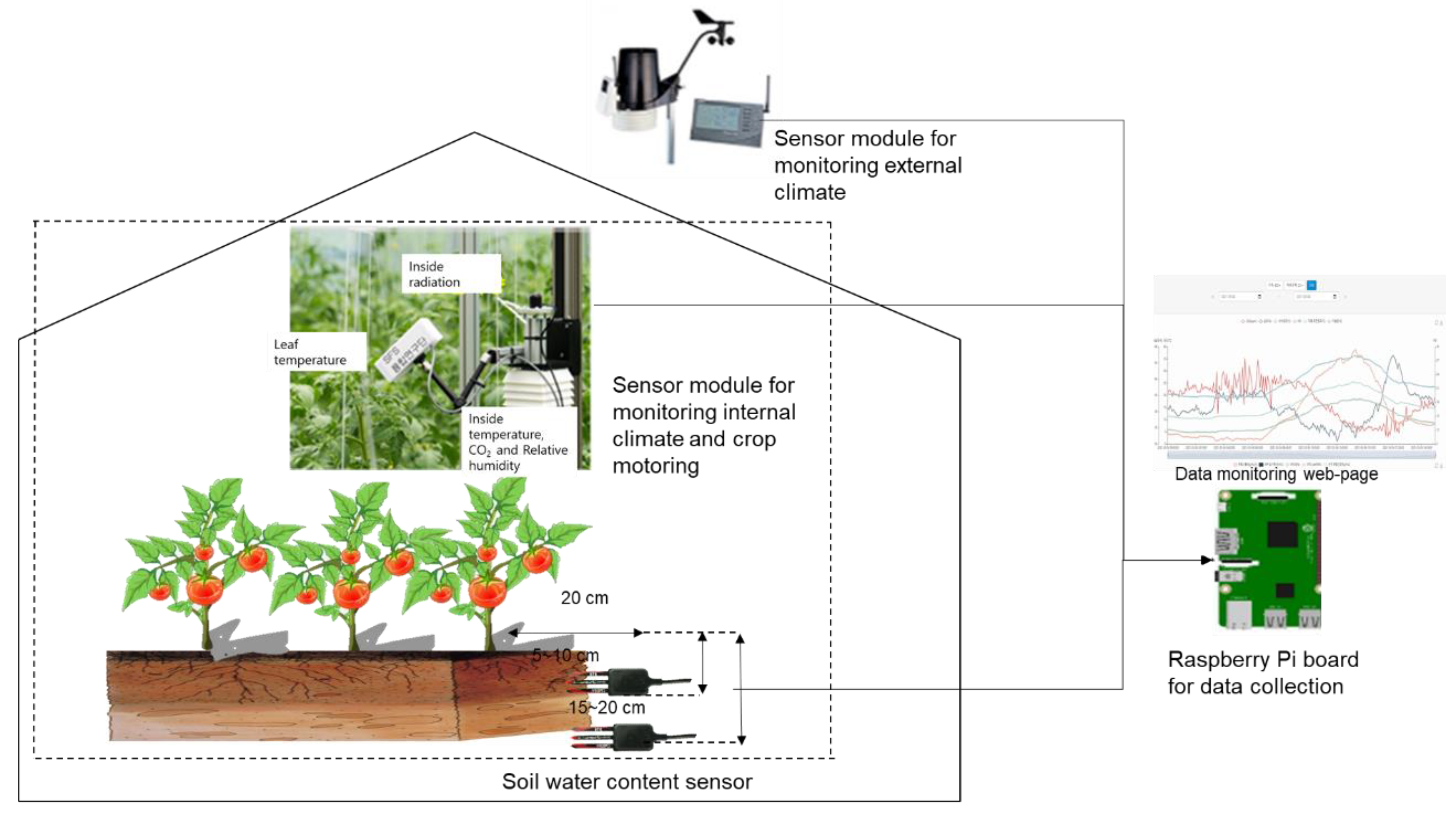
2.1. Greenhouse and Sensor Description

The experiment was carried out in a Venlo-type multi-greenhouse located in an experimental horticulture field in Gangneung, South Korea. The greenhouse structure had four consecutive Venlo-type sections to constitute a total area of 800 m², of which the cultivated soil of 200 m² was set as the experimental area in this study. In this area, tomato (Athene cultivar) was cultivated. The system for the collection of data used in this study is illustrated in Figure 1. A climate sensor module (SH-VT260, SOHA-tech, Seoul, Korea) inside the greenhouse for the temperature, humidity, and CO₂ and an infrared temperature sensor for measuring the leaf surface temperature located at the height of growing point of the tomato plant were installed. An external sensor module to monitor the climatic conditions outside the greenhouse (Vantage Pro2, Avis Instruments, CA, USA) was set up to collect temperature, humidity, wind direction and velocity data outside the greenhouse. To measure the soil moisture, a 5TE sensor (5TE, Decagon Devices Inc., Pullman, WA, USA) was installed. Two sensors were installed at depths of 5–10 cm and 15–20 cm, horizontal to the crop (Figure 1). These sensors were vertically aligned with the dripper point where the nutrient solution was irrigated to ensure the changes in soil water content could be rapidly incorporated.

As the history of operation of the actuators that modulate the environment inside the greenhouse is a critical factor, the respective data were also collected for use in developing the prediction model.

Table 1. Input variable, unit, and range used to develop ET prediction model.

Input Variables (Unit)	Min–Max
Outside temperature (°C)	15.5–29.9
Outside humidity (%)	41.5–100
Outside CO2 concentration (ppm)	355.2–443.0
Radiation (W/m2)	0–1355.4
Wind speed (m/s)	0–3.81
Shade curtain (%)	0–100
Circulating Fan	0 or 1
Heating valve (%)	0–100
Fogging	0 or 1
CO2 injection	0 or 1
Heat retention curtain (%)	55–100
Soil temperature (°C)	14.6–30.1
Left and right window openness (%)	0–100
Wind direction (°)	0–359
Inside humidity (%)	36.1–99.1
Inside CO2 concentration (ppm)	351.2–1124.6
Inside temperature (°C)	19.6–35.1
Leaf temperature (°C)	16.5–33.6
Volumetric water contents of soil (%)	5.53–38.5

presents the information regarding the applied sensor and actuator signals. This study was conducted from 15 May to 22 June by collecting data, and data from 1 June to 22 June was used for model training and validation.

2.2. Development of an ET Prediction Model

2.2.1. A Prediction Model for ET in a Tomato Greenhouse

The Stanghellini [13] model was extended to the whole plant, focusing on energy exchange from the leaves in order to apply the model in a greenhouse environment. By applying LAI, an attempt was made to consider the radiation absorption of the multi-layered canopy. Individual leaf length and maximum width were manually measured weekly on 10 randomly selected plants. LAI was determined by multiplying the maximum width and leaf length and a reduction coefficient of 0.64 [28,29]. LAI started measuring after the first flowering flower cluster was created, and the data set used in this study was carried out at the harvest time of the third flower cluster, about 12 to 15 weeks after planting.

Table 2. Symbol and unit for the various variables used to calculate the evapotranspiration rate of the Stanghellini model [14].

Symbol	Variables	Unit
E	Evapotranspiration rate	Kg/s ∙ m2∙canopy area
Tair	Ambient air temperature	°C
To	Temperature at the leaf surface	°C
RH	Relative humidity	%
Is	Shortwave irradiance	W/m2
LAI	Leaf area index; the ratio of the total leaf area (one side) to the canopy area, 2.5–3.5 in this study	m2/m2
L	Latent heat of the vaporization of water, 2,502,535.239–2385.76 ∙ Tair	J/kg
ρa	Air density, 100,000/287∙(Tair + 273.16)	Kg/m3
cp	Air specific heat at constant pressure, 1013	J/kg/°C
δ	Slope of the saturation vapor pressure–temperature curve, 41.45 exp(0.06088 ∙ Tair)	Pa/°C
γ	Psychometric constant, $\frac{c_p}{L} \frac{P_{atm}}{0.6216}$	Pa/°C
$P_{atm}$	Atmospheric pressure, 101,325 ${\left(\frac{293-0.0065 ·h}{293}\right)}^{5.26}$	Pa
h	Elevation above sea level, 70 m
ri	Internal resistance of the canopy to vapor transfer $r_i=\frac{I_s+4.30}{I_s+0.54}[1+2.3·{10}^{-2}{\left(T_0-24.5\right)}^2]·{\tilde{r}}_i\left(C{O}_2\right)·{\tilde{r}}_i\left(e_a^{*}-e_a\right)$ ${\tilde{r}}_i\left(C{O}_2\right)\begin{array}{c}=1,I_s=0 W·m^{-2}\\ =1+6.1·{10}^{-7}{\left(C{O}_2-200\right)}^2,C{O}_2<1100 ppm\\ =1,C{O}_2 \ge 1100 ppm\end{array}$ ${\tilde{r}}_i\left(e_a^{\text{*}}-e_a\right)\begin{array}{c}=1+4.3·{\left(e_a^{\text{*}}-e_a\right)}^2,e_a^{\text{*}}-e_a<0.8kPa\\ =3.8,e_a^{\text{*}}-e_a\ge 0.8kPa\end{array}$	S/m
re	External resistance of the canopy to sensible heat transfer, $u$ is the friction velocity (m·s−1) $r_e=\frac{1174 l^{0.5}}{{\left(l\left|T_0-T_a\right|+207 u^2\right)}^{0.25}}$
Th	Apparent temperature of the ambient environment as determined by the pipe, floor, and cladding temperature, Tair
rR	Linearization factor of the radiation heat flux equation, $\frac{{\rho }_a{c}_p}{4·\sigma ·{\left(T_a+273.15\right)}^3} \left[s m^{-1}\right]$
σ	Stefan–Boltzmann constant, 5.669 × 10−8	J/K4/m2/s
ea*	Saturation vapor pressure at mean air temperature, $610.78·exp\left(\frac{17.269·T_{air}}{237.3+T_{air}}\right)\left[Pa\right]$	Pa
ea	Vapor pressure at air temperature, $e_a^{*}\frac{RH}{100} \left[Pa\right]$	Pa

shows the constant values and definitions of the variables of the applied Stanghellini model.

$$LE \cong \frac{2·LAI·{\rho }_a{c}_p}{\gamma ·\left(r_i+r_e\right)} \left(VPD\right)$$

(1)

Here, Equation (1) can be converted to

$$LE \cong \frac{2·LAI·{\rho }_a{c}_p}{1+\frac{\delta }{\gamma }+\frac{r_i}{r_e}}\left[0.07\frac{\delta }{\gamma }\frac{I_s}{{\rho }_a{c}_p}+0.16\frac{\delta }{\gamma }\frac{T_h-T_o}{r_R}+\frac{1}{r_e}\frac{e_a^{*}-e_a}{\gamma }\right]$$

(2)

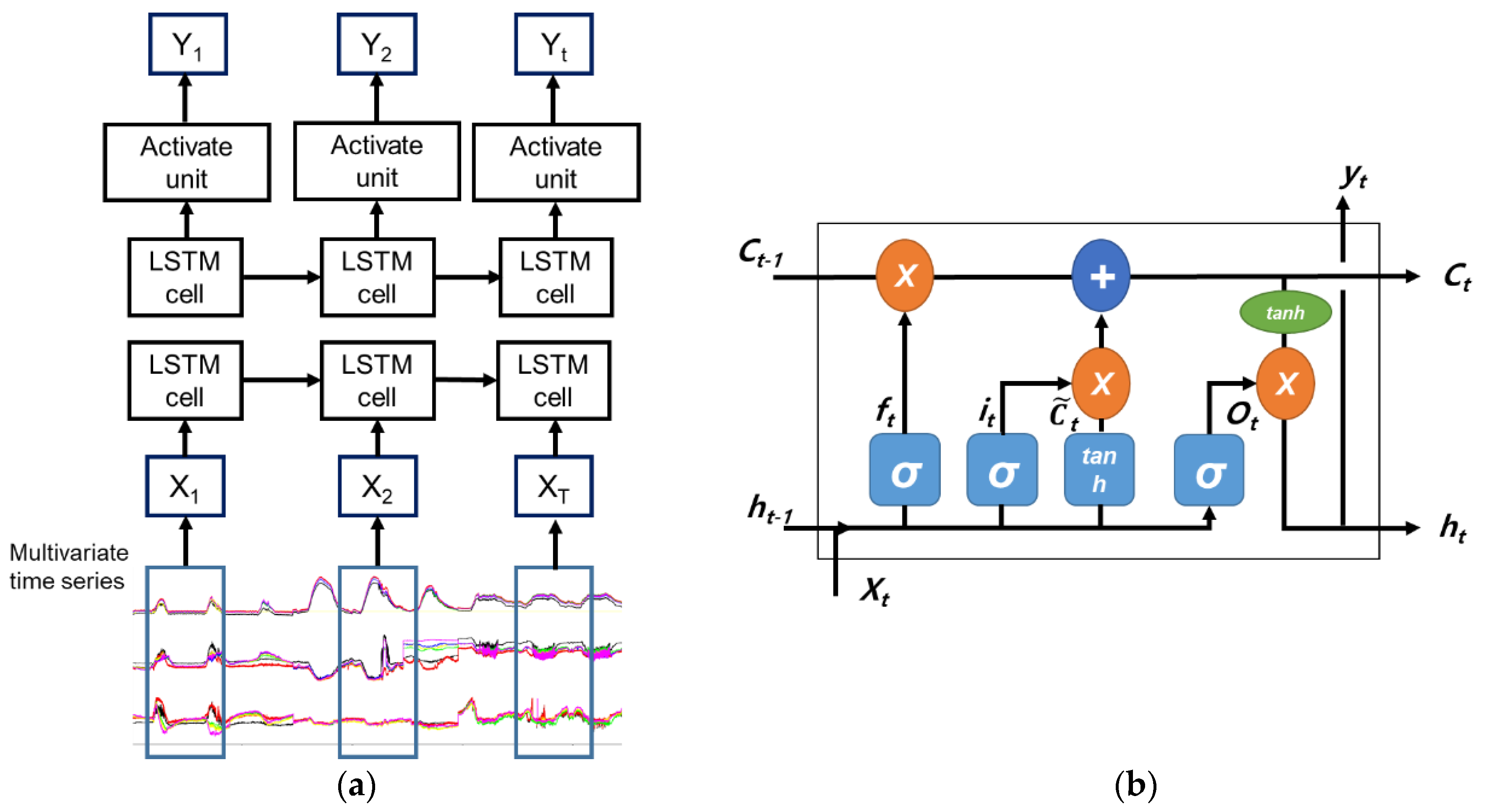
2.2.2. An LSTM-Based ET Prediction Model

The LSTM model suggested in a previous study [4] as a suitable algorithm to predict the environment inside the greenhouse was applied in this study for comparison with the prediction model for ET. The overall structure of the RNN-based prediction model is shown in Figure 2a, while Figure 2b shows the detailed structure of the LSTM device used in this study.

An advantage of LSTM is its strength relative to long-term memory loss. Hence, it was adopted in this study as the input data in model training for humidity prediction exhibiting a time-series structure. The interior of LSTM comprises a forget gate, an input gate, a sigmoid output gate and a cell state; the details of the computation are described in Hochreiter and Schmidhuber [30]. The LSTM model as a result constituted a multivariate model with the 19 sensor and actuator signals (Table 1). The output was the ET data from the Stanghellini model that was used for the training. The data used in training were collected in 5 min intervals, and multi-step prediction was applied. The training model consisted of two layers; a rectified linear unit (ReLu layer and an LSTM layer, while the linear function was applied in the activated unit. The mean absolute error (MAE) was used in loss function, and Adam was applied in optimization. The training was performed for 20 epochs. The prediction performance was compared independently for the training and the test sets.

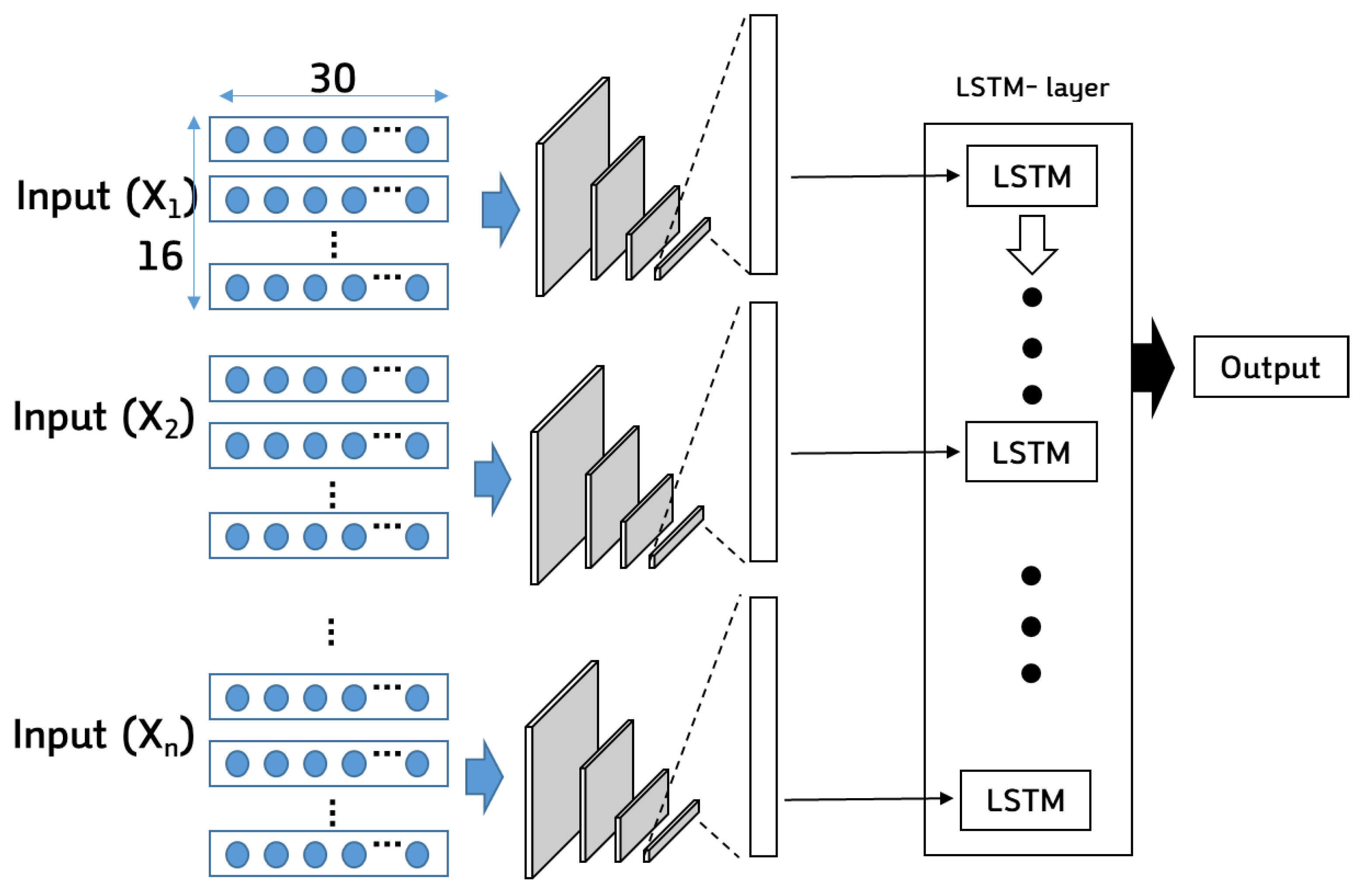
2.3. A CNN-LSTM-Based Humidity Prediction Model

The goal of the humidity prediction model was to predict the change in humidity within 30 min of the current humidity. For humidity prediction, the model was based on the CNN structure to which the input data were fed. Three versions of the CNN model were used in the training using the data of 20 days between 1 June and 19 June. The model was validated using the subsequent 4-day environmental data.

Table 3. The datasets used for the humidity prediction model.

CNN Models	Input Data
Model-1	Micro-climate sensor of inside the greenhouse, external weather information, and operation signals of actuators inside the greenhouse.
Model-2	A dataset with evapotranspiration information added to the dataset of Model-1.
Model-3	A dataset with tomato leaf temperature sensor and soil moisture sensor, leaf vapor-pressure deficit, and dew points added to Model-1.

describes the classification of data fed to the three CNN models. First, for Model-1, the sensor data including the environmental data used in conventional humidity prediction and the signal data of the greenhouse actuator operation were used. For Model-2, the data of ET from the previously developed Stanghellini model were added to the data used for Model-1. For Model-3, further data from the root-zone sensing and leaf temperature sensing were added. Soil volumetric water content (VWC) and soil temperature were measured with a root zone sensor. In addition, the dew point values were determined through the humidity sensor near the crop and the leaf temperature sensor. During the experiment, the dew points ranged from 8.4 to 20.1 °C. In testing each model with respect to the prediction of the humidity inside the greenhouse, the conventional environmental data and the data from the greenhouse actuators were compared, and the ET or respective root-zone and crop monitoring sensing parts were comparatively analyzed based on model outcomes regarding their importance as a factor related to humidity variation. An additional comparison was made with the RNN-LSTM model proposed in a previous study [4]. The set of input variables was identical to the case of Model-1. The model training was conducted through further tuning of the previously trained model.

The environmental and control history data collected in the greenhouse were used to develop a model using the CNN structure and LSTM device in the deep learning-based prediction technologies. A CNN consists of an input and an output layer, as well as multiple hidden layers (Figure 3). The hidden layers of a CNN typically consist of a series of convolutional layers that interact with a multiplication or another dot product. For building a CNN model, a value without a filter feature becomes a value close to 0, and since this value comes out as a numerical value, it must be changed to a non-linear value of 0 or 1. This is called the activation function, and the ReLu function is commonly used in deep learning models. A method of artificially reducing the feature map generated through the activation function is called pooling, and in this study, max pooling was applied. A fully connected layer was placed on processing the feature values obtained from multiple convolutional layers with an artificial neural network (Figure 3).

A deep learning model with a CNN with LSTM was used as the basic structure of the environmental model in this study. Figure 3 presents the overall structure of the model. About 30 consecutive data points were used as input data, and the array was a two-dimensional (2D) [14]. The kernel size was (1,3), and a total of 4 composite layers were used for the 2D convolutional layer. The max pooling size for each layer was (1,2), (2,2), and (1,2). A total of 15 nodes in the dense layer was used, and ReLu was chosen as the active function. Model training was performed with 100 epochs and 5 batch sizes [14]. The default value of AdaDelta was set to the optimization function, which is widely used as a stochastic gradient descent method. Each floor was given a dropout rate of 25% to contribute to the learning rate. LSTM architecture is an efficient way to eliminate memory loss in continuous time series data.

An optimal comparison of prediction models was achieved on the coefficient of determination (R²) that identifies the correlation between the actual measured data and the prediction data. For measures of dispersion, the standard error of prediction (%SEP) and the root mean squared error (RMSE) were compared (Equations (4) and (5)). The comparison was used in determining the method that provides an adequate explanation for the total dispersion of data by the model.

$${\mathrm{R}}^2=1-\frac{\mathrm{SSE}}{\mathrm{SSTO}}=1-\frac{{{\displaystyle \sum }}_{\mathrm{i}=1}^{\mathrm{n}}{\left({\mathrm{X}}_{\mathrm{obs},\mathrm{i}}-{\mathrm{X}}_{\mathrm{model},\mathrm{i}}\right)}^2}{{{\displaystyle \sum }}_{\mathrm{i}=1}^{\mathrm{n}}{\left({\mathrm{X}}_{\mathrm{obs},\mathrm{i}}-{\overline{\mathrm{X}}}_{\mathrm{obs},\mathrm{i}}\right)}^2}$$

(3)

$$\mathrm{RMSE}=\sqrt{\frac{1}{\mathrm{N}}{{\displaystyle \sum }}_{\mathrm{i}=1}^{\mathrm{n}} {\left({\mathrm{X}}_{\mathrm{obs},\mathrm{i}}-{\mathrm{X}}_{\mathrm{model},\mathrm{i}}\right)}^2 }$$

(4)

$$\mathrm{SEP} (\%)=\frac{100}{{\overline{\mathrm{X}}}_{\mathrm{obs},\mathrm{i}}}\sqrt{\frac{1}{\mathrm{N}}{{\displaystyle \sum }}_{\mathrm{i}=1}^{\mathrm{n}} {\left({\mathrm{X}}_{\mathrm{obs},\mathrm{i}}-{\mathrm{X}}_{\mathrm{model},\mathrm{i}}\right)}^2 }$$

(5)

3. Results

3.1. Comparison of ET Prediction Model Outcomes

The ET prediction model outcomes were obtained after the training of the LSTM model (using an approximately 20-day dataset) and the testing (using an approximately 3-day dataset) for the comparison of prediction accuracy. The ET prediction model for actual values was the Stanghellini model for the internal ET in tomato greenhouses. The RMSE between the actual and the predicted values of the LSTM model used in training was 0.00317 kgm⁻² s⁻¹, and the RSME for the predicted values after applying the model to the test set was 0.00356 kgm⁻² s⁻¹. Through conversion to % SEP for comparison, the respective errors were 5.76 and 6.45%. This verified the possibility of the deep learning model interpretation of ET using the sensors and the environmental control data in greenhouses and an additional device for the crop leaf temperature monitoring. Figure 4 shows the results of the training data set and the test data set of the two models.

3.2. Comparison of Humidity Prediction Model Outcomes

For the humidity prediction model, the data of 20 days between 1 June and 19 June were used in training, after which a 1:1 comparison with actual values was conducted (Figure 5). In the training stage, all three models produced an R² of more than 0.90 (Figure 5), with the highest observed for Model-3 (0.98). Model-2, including ET data, showed the best performance with an RMSE of 1.99 in the test set. Overall, the standard error of prediction (SEP) improved from 5.59% in Model-1 to 3.26 and 2.67% for Models-2 and -3, respectively (Figure 5). The values from the prediction model and the measured values for the displacement between the actual change in humidity and the current humidity were compared (Figure 6). As the goal in this study was to ultimately identify the change in humidity 30 min into the future, the final model performance can be accounted for by Figure 6. The difference between the actual measured humidity and the humidity measured after 30 min was calculated, which was taken as the X-axis for a 1:1 comparison with the humidity after 30 min as predicted by the model. Consequently, the coefficient of determination for Model-1 was 0.58, while that for Model-2 was 0.76 and that for Model-3 was 0.84. In the prediction of humidity, therefore, the data from Model-2 and Model-3 were better. Based on these results, it can be seen that the humidity in the greenhouse is closely linked to the ET rate. The more moisture-related information a greenhouse could help to develop, the more precise the humidity prediction model. In addition, the hybrid deep-learning model considered along with the physical model could help more precise model development.

The performances of the final three models developed in this study were compared using the test set data. The actual and predicted values of changes in humidity between 20 June and 24 June, the time set apart as the test set, were compared (Figure 7). In addition, the RNN-LSTM model from a previous study [4] was used on the test set for humidity prediction, where the set of input variables was identical to the case of Model-1. The prediction performance of the test set was higher than in the training set in terms of RMSE. Notably, the RMSE was 4.22 for the CNN Model-1 using the environmental data only, whereas the RMSEs for Model-2 and Model-3 were 3.02 and 2.87, respectively. As with training outcomes, the CNN Model-3 displayed the highest prediction performance. The comparison with the RNN-LSTM model was possible for the CNN Model-1 using the same input data, and the CNN model was shown to be slightly higher in predictive performance.

4. Discussion

The moisture balance in a greenhouse is influenced by the external climatic conditions, the plant, the soil and other environmental factors, unless it is a completely sealed system. Thus, the balanced moisture control is known to pose critical as well as challenging tasks alongside the control of greenhouse temperature [31,32,33]. In this light, the findings in this study verified the potential use of a data-based approach for the modeling of ET in tomato greenhouses. Notably, previous study [34] reported that using a humidity prediction model of tomato greenhouses may allow the climatic variables, such as the set point of temperature or ventilation, to be inferred in the process of crop cultivation to the desired level, thereby concluding that modern greenhouse climate control should integrate various humidity models towards the goal of overseeing the entire process of crop cultivation. In the same way, the external and internal climatic data that may be generalized in modern greenhouses as well as the data of commercially available devices such as the actuator operation data were used in this study to achieve a level of precision for the ET prediction model close to the Stanghellini model, which was a positive outcome in verifying the potential use of such data. However, in data-based modeling, the limitation seems to be the difference between the actual and predicted ET as the precise measurements of ET could not be used in training.

The modeling of the humidity inside the greenhouse has been conducted in numerous studies. Nevertheless, simple and sophisticated modeling is known to be difficult due to the influence of various external factors [5,18,35]. With advanced processing speeds, data-based modeling has been widely applied across fields with deep learning based on an RNN or CNN structure, which has led to an improvement in the performance of greenhouse environment models. Notably, a previous study [4] reporting on time-series modeling such as NARX and RNN, showed performance to be uncertain for humidity prediction compared to temperature or CO₂ prediction. To resolve such limitations in the current study, first, the crop ET was monitored and used as a variable. The trend of change in ET may be regarded as a critical factor in the variation in humidity inside the greenhouse. Without using precise ET data, the results in this study showed that the performance could be adequately improved through the use of the data of tomato leaf temperature, root-zone sensors, and soil water content sensors as variables. Second, such data were fed to a 2D, CNN input structure in the RNN-based time series modeling, and through the addition of an LSTM device, memory function based on time series was suggested for the modeling structure. Compared to the conventional use of RNN or LSTM alone, the structure with the 2D convolution layer for primary modeling of data patterns, followed by the time series interpretation, is likely to have contributed to enhancing the predictive performance.

For these approaches of a data-based modeling of the greenhouse environment to facilitate the sharing of the trained models without adjustments, there are numerous practical issues. As the data to be used would vary according to the greenhouse or field conditions, and the structure of the facility or the microenvironment are the key factors, it is difficult to apply a generalized trained model through conventional micro-tuning. However, a data-based modeling approach is anticipated to lead to modeling through training with the continuous collection of greenhouse or agricultural field data. Such environmental modeling appears adequate for use in a controlled engineering approach to ultimately satisfy the optimal environment conditions in agricultural facilities or greenhouses.

5. Conclusions

This study designed data-based, deep-learning models for the modeling of crop ET and variation in humidity in tomato greenhouses using the greenhouse environment and actuator data. The model performance was compared, and the results are summarized as follows:

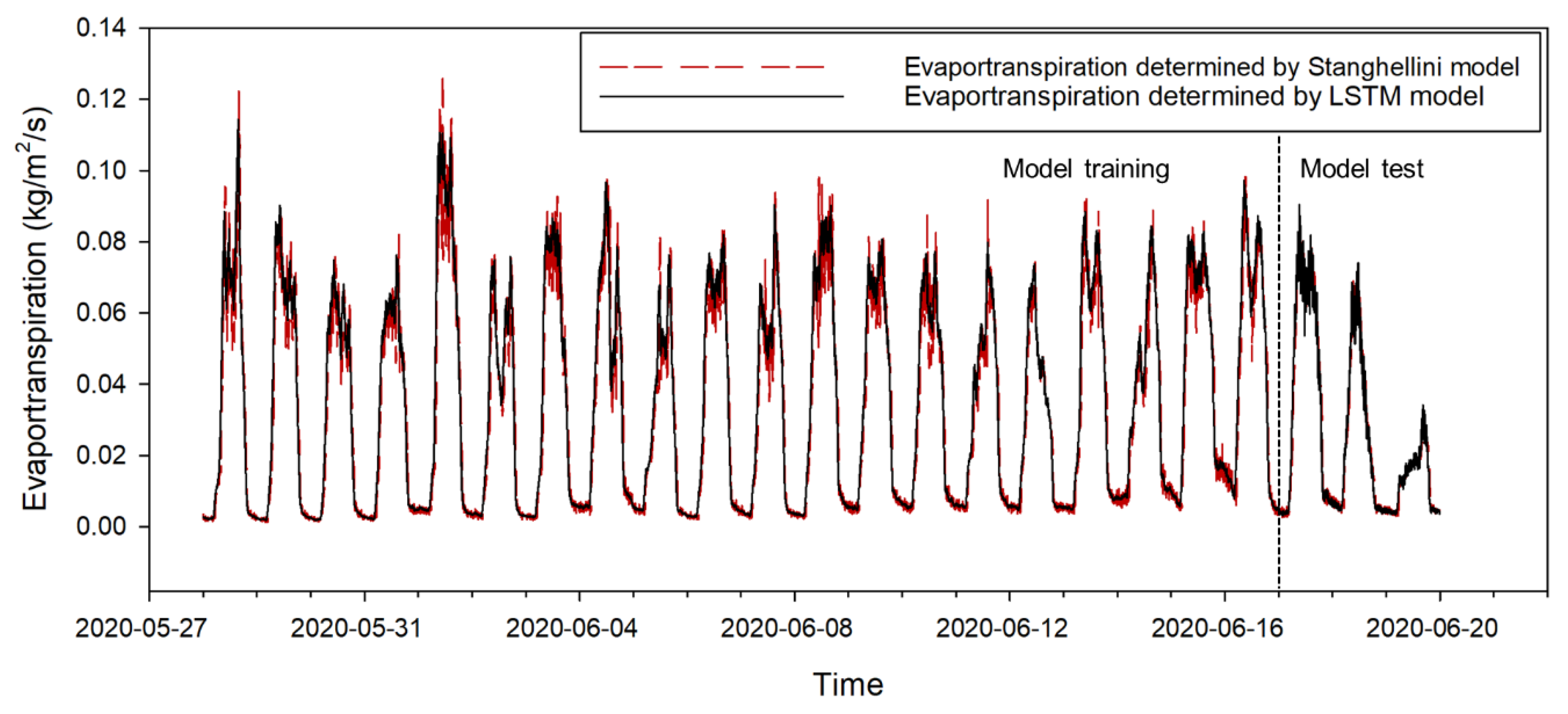
• An ET prediction model was developed through LSTM modeling using time series data. For this, the crop root-zone and leaf temperature sensors were additionally installed to apply the Stanghellini model. The ET data from the Stanghellini model were used in the training of the LSTM model. The training set contained the data of 20 days and the test set contained the data of 3 days, for subsequent comparison with the Stanghellini model outcomes. In training, the RMSE for the two values was 0.00317 kgm⁻² s⁻¹, and the RMSE for the predicted values after applying the model to the test set was 0.00356 kgm⁻² s⁻¹. The errors indicated by %SEP were 5.76 and 6.45%, respectively.
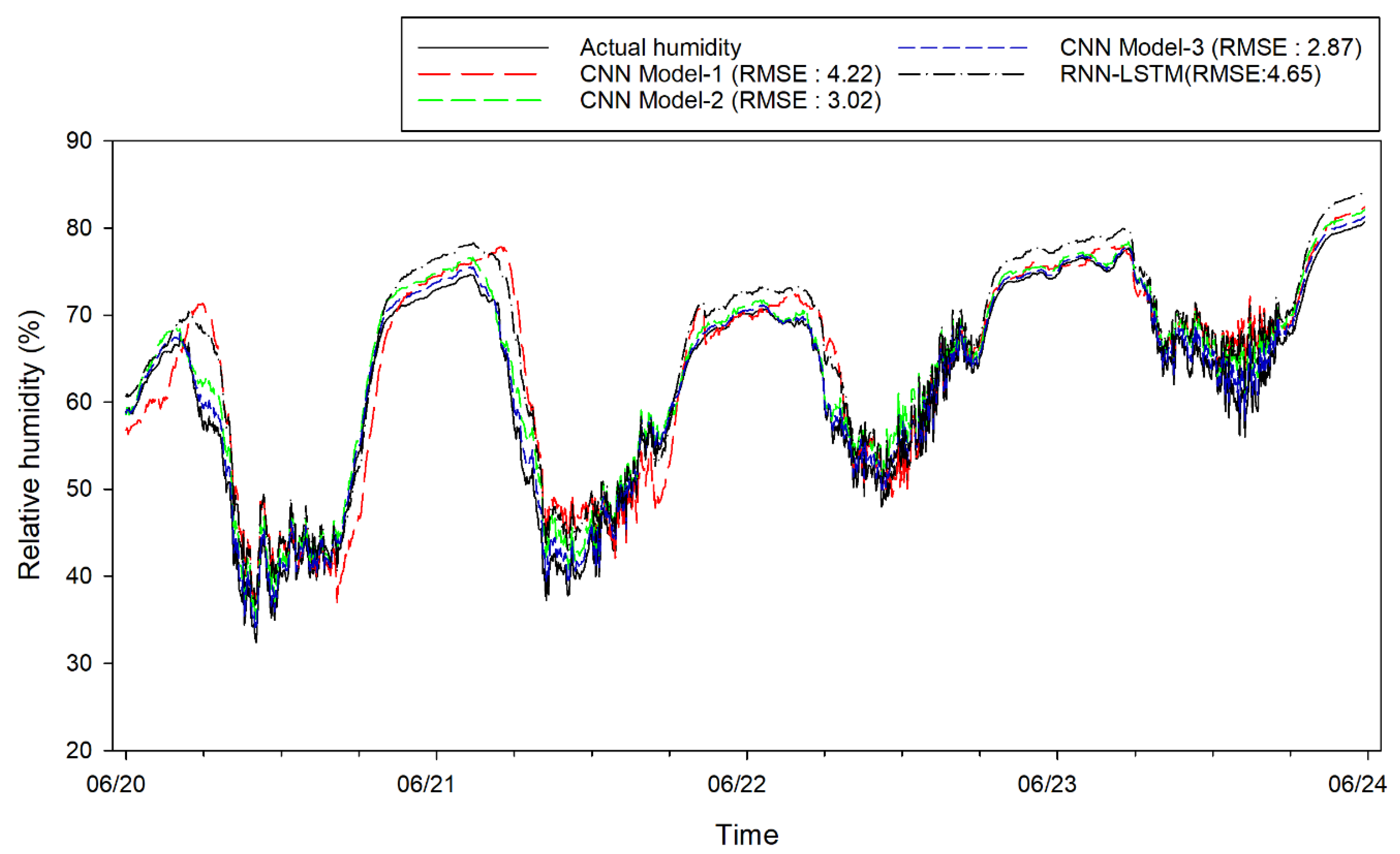
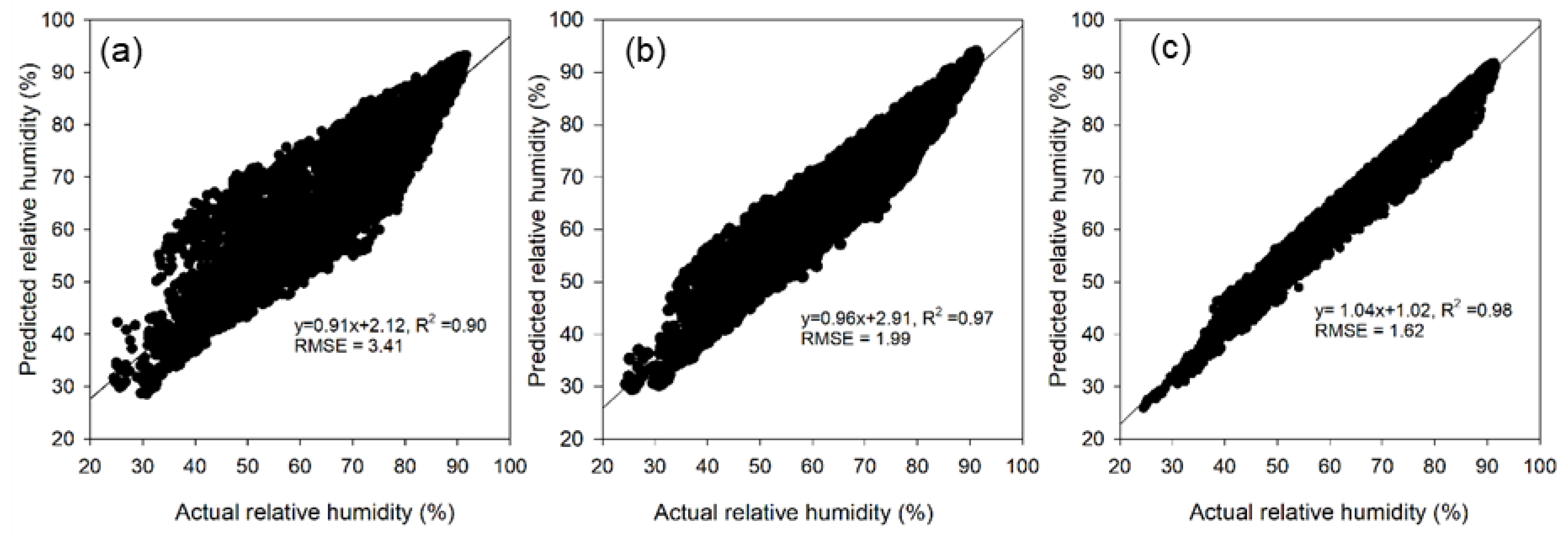
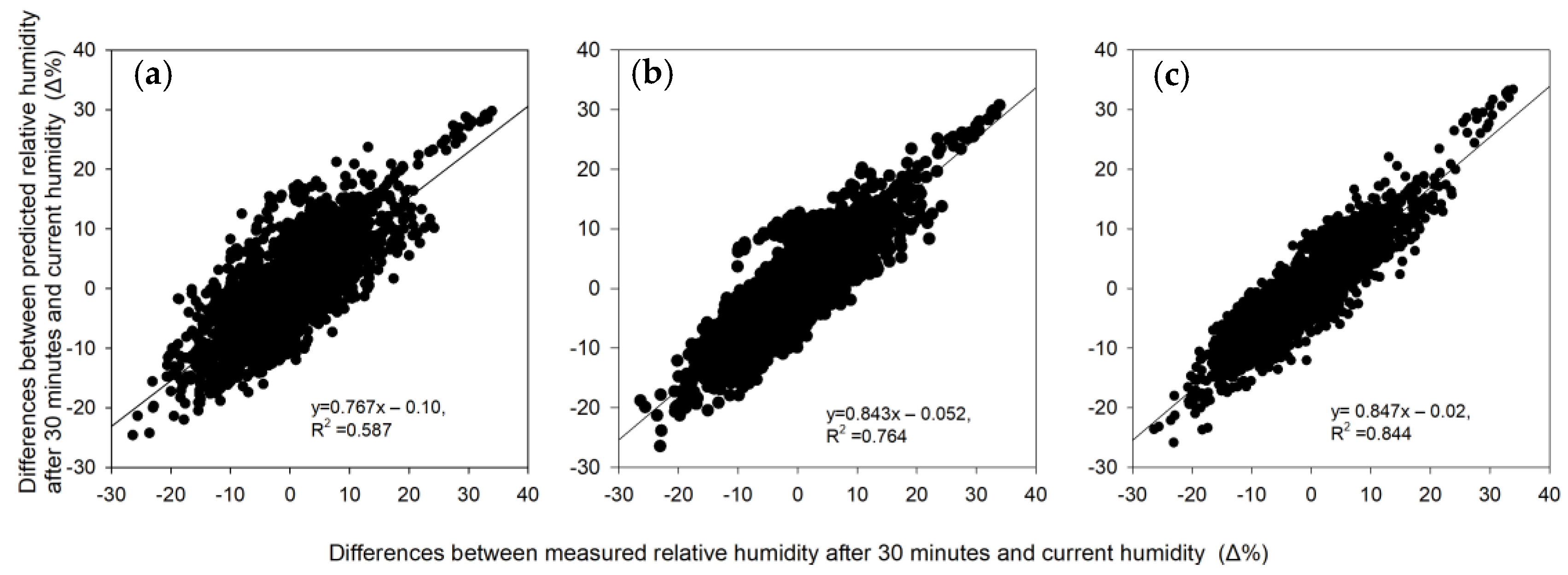
• A humidity prediction model was developed to predict the current change in humidity inside the greenhouse, i.e., the humidity 30 min into the future. The input data included the various greenhouse environmental data, the history of actuator operation, the ET, the soil sensor, and crop environment data, which were fed as multiple variables to the 2D CNN structure via the convolution layer in continuous time. This was connected to the LSTM structure to finalize the modeling. The results showed that the RMSE for the predicted values of the test set was 2.87, confirming a better level of performance than the conventional RNN-LSTM model.

The findings in this study are anticipated to contribute to providing optimal control of the greenhouse internal environment; the data will be useful in the modeling and control studies to ensure a greenhouse environment that satisfies various critical environmental conditions including temperature, humidity, and CO₂.

References

1. He, F.; Ma, C. Modeling Greenhouse Air Humidity by Means of Artificial Neural Network and Principal Component Analysis. Comput. Electron. Agric. 2010, 71, S19–S23. [Google Scholar] [CrossRef]
2. El Ghoumari, M.Y.; Tantau, H.J.; Serrano, J. Non-Linear Constrained MPC: Real-Time Implementation of Greenhouse Air Temperature Control. Comput. Electron. Agric. 2005, 49, 345–356. [Google Scholar] [CrossRef]
3. Seginer, I.; McClendon, R.W. Methods for Optimal Control of the Greenhouse Environment. Trans. ASAE 1992, 35, 1299–1307. [Google Scholar] [CrossRef]
4. Jung, D.-H.; Kim, H.S.; Jhin, C.; Kim, H.-J.; Park, S.H. Time-Serial Analysis of Deep Neural Network Models for Prediction of Climatic Conditions inside a Greenhouse. Comput. Electron. Agric. 2020, 173, 105402. [Google Scholar] [CrossRef]
5. Castañeda-Miranda, A.; Castaño, V.M. Smart Frost Control in Greenhouses by Neural Networks Models. Comput. Electron. Agric. 2017, 137, 102–114. [Google Scholar] [CrossRef]
6. Ferreira, P.M.; Faria, E.A.; Ruano, A.E. Neural Network Models in Greenhouse Air Temperature Prediction. Neurocomputing 2002, 43, 51–75. [Google Scholar] [CrossRef]
7. Hongkang, W.; Li, L.; Yong, W.; Fanjia, M.; Haihua, W.; Sigrimis, N.A. Recurrent Neural Network Model for Prediction of Microclimate in Solar Greenhouse. IFAC-PapersOnLine 2018, 51, 790–795. [Google Scholar] [CrossRef]
8. Anapalli, S.S.; Ahuja, L.R.; Gowda, P.H.; Ma, L.; Marek, G.; Evett, S.R.; Howell, T.A. Simulation of Crop Evapotranspiration and Crop Coefficients with Data in Weighing Lysimeters. Agric. Water Manag. 2016, 177, 274–283. [Google Scholar] [CrossRef]
9. Chen, J.; Xu, F.; Tan, D.; Shen, Z.; Zhang, L.; Ai, Q. A Control Method for Agricultural Greenhouses Heating Based on Computational Fluid Dynamics and Energy Prediction Model. Appl. Energy 2015, 141, 106–118. [Google Scholar] [CrossRef]
10. Chiew, F.H.S.; Kamaladasa, N.N.; Malano, H.M.; McMahon, T.A. Penman-Monteith, FAO-24 Reference Crop Evapotranspiration and Class-A Pan Data in Australia. Agric. Water Manag. 1995, 28, 9–21. [Google Scholar] [CrossRef]
11. Beven, K. A Sensitivity Analysis of the Penman-Monteith Actual Evapotranspiration Estimates. J. Hydrol. 1979, 44, 169–190. [Google Scholar] [CrossRef]
12. Katsoulas, N.; Stanghellini, C. Modelling Crop Transpiration in Greenhouses: Different Models for Different Applications. Agronomy 2019, 9, 392. [Google Scholar] [CrossRef]
13. Stanghellini, C. Transpiration of Greenhouse Crops: An Aid to Climate Management; Agricultural University: Wageningen, The Netherlands, 1987. [Google Scholar]
14. Dae-Hyun, J. Development of Artificial Intelligence-Based Climate Control System for Smart Greenhouse. Ph.D. Thesis, Seoul National University, Seoul, Korea, August 2020. [Google Scholar]
15. Yan, H.; Huang, S.; Zhang, C.; Gerrits, M.C.; Wang, G.; Zhang, J.; Zhao, B.; Acquah, S.J.; Wu, H.; Fu, H. Parameterization and Application of Stanghellini Model for Estimating Greenhouse Cucumber Transpiration. Water 2020, 12, 517. [Google Scholar] [CrossRef]
16. Villarreal-Guerrero, F.; Kacira, M.; Fitz-Rodríguez, E.; Kubota, C.; Giacomelli, G.A.; Linker, R.; Arbel, A. Comparison of Three Evapotranspiration Models for a Greenhouse Cooling Strategy with Natural Ventilation and Variable High Pressure Fogging. Sci. Hortic. 2012, 134, 210–221. [Google Scholar] [CrossRef]
17. Orgaz, F.; Fernández, M.D.; Bonachela, S.; Gallardo, M.; Fereres, E. Evapotranspiration of Horticultural Crops in an Unheated Plastic Greenhouse. Agric. Water Manag. 2005, 72, 81–96. [Google Scholar] [CrossRef]
18. Villarreal-Guerrero, F.; Kacira, M.; Fitz-Rodríguez, E.; Linker, R.; Kubota, C.; Giacomelli, G.A.; Arbel, A. Simulated Performance of a Greenhouse Cooling Control Strategy with Natural Ventilation and Fog Cooling. Biosyst. Eng. 2012, 111, 217–228. [Google Scholar] [CrossRef]
19. Stanghellini, C. Environmental Control of Greenhouse Crop Transpiration. J. Agric. Eng. Res. 1992, 51, 297–311. [Google Scholar] [CrossRef]
20. Pahuja, R.; Verma, H.K.; Uddin, M. An Intelligent Wireless Sensor and Actuator Network System for Greenhouse Microenvironment Control and Assessment. J. Biosyst. Eng. 2017, 42, 23–43. [Google Scholar] [CrossRef]
21. Pahuja, R.; Verma, H.K.; Uddin, M. Implementation of Greenhouse Climate Control Simulator Based on Dynamic Model and Vapor Pressure Deficit Controller. Eng. Agric. Environ. Food 2015, 8, 273–288. [Google Scholar] [CrossRef]
22. Taki, M.; Ajabshirchi, Y.; Ranjbar, S.F.; Rohani, A.; Matloobi, M. Heat Transfer and MLP Neural Network Models to Predict inside Environment Variables and Energy Lost in a Semi-Solar Greenhouse. Energy Build. 2016, 110, 314–329. [Google Scholar] [CrossRef]
23. Jung, D.-H.; Kim, H.-J.; Kim, S.H.; Choi, J.; Kim, D.J.; Park, H.S. Fusion of Spectroscopy and Cobalt Electrochemistry Data for Estimating Phosphate Concentration in Hydroponic Solution. Sensors 2019, 19, 2596. [Google Scholar] [CrossRef] [PubMed]
24. Zou, W.; Yao, F.; Zhang, B.; He, C.; Guan, Z. Verification and Predicting Temperature and Humidity in a Solar Greenhouse Based on Convex Bidirectional Extreme Learning Machine Algorithm. Neurocomputing 2017, 249, 72–85. [Google Scholar] [CrossRef]
25. Ge, J.; Zhao, L.; Yu, Z.; Liu, H.; Zhang, L.; Gong, X.; Sun, H. Prediction of Greenhouse Tomato Crop Evapotranspiration Using XGBoost Machine Learning Model. Plants 2022, 11, 1923. [Google Scholar] [CrossRef]
26. Shin, J.H.; Park, J.S.; Son, J.E. Estimating the Actual Transpiration Rate with Compensated Levels of Accumulated Radiation for the Efficient Irrigation of Soilless Cultures of Paprika Plants. Agric. Water Manag. 2014, 135, 9–18. [Google Scholar] [CrossRef]
27. Meftah, O.; Guergueb, Z.; Braham, M.; Sayadi, S.; Mekki, A. Long Term Effects of Olive Mill Wastewaters Application on Soil Properties and Phenolic Compounds Migration under Arid Climate. Agric. Water Manag. 2019, 212, 119–125. [Google Scholar] [CrossRef]
28. Liu, H.; Sun, J.S.; Duan, A.W.; Sun, L.; Liang, Y.Y. Simple Model for Tomato and Green Pepper Leaf Area Based on AutoCAD Software. Chin. Agric. Sci. Bull. 2009, 25, 287–293. [Google Scholar]
29. Gong, X.; Qiu, R.; Zhang, B.; Wang, S.; Ge, J.; Gao, S.; Yang, Z. Energy Budget for Tomato Plants Grown in a Greenhouse in Northern China. Agric. Water Manag. 2021, 255, 107039. [Google Scholar] [CrossRef]
30. Hochreiter, S.; Schmidhuber, J. Long Short-Term Memory. Neural Comput. 1997, 9, 1735–1780. [Google Scholar] [CrossRef]
31. Tawegoum, R.; Teixeira, R.; Chasseriaux, G. Simulation of Humidity Control and Greenhouse Temperature Tracking in a Growth Chamber Using a Passive Air Conditioning Unit. Control Eng. Pract. 2006, 14, 853–861. [Google Scholar] [CrossRef]
32. Körner, O.; Challa, H. Process-Based Humidity Control Regime for Greenhouse Crops. Comput. Electron. Agric. 2003, 39, 173–192. [Google Scholar] [CrossRef]
33. Guo, Y.; Zhao, H.; Zhang, S.; Wang, Y.; Chow, D. Modeling and Optimization of Environment in Agricultural Greenhouses for Improving Cleaner and Sustainable Crop Production. J. Clean. Prod. 2021, 285, 124843. [Google Scholar] [CrossRef]
34. Stanghellini, C.; de Jong, T. A Model of Humidity and Its Applications in a Greenhouse. Agric. For. Meteorol. 1995, 76, 129–148. [Google Scholar] [CrossRef]
35. González Perea, R.; Camacho Poyato, E.; Montesinos, P.; Rodríguez Díaz, J.A. Optimisation of Water Demand Forecasting by Artificial Intelligence with Short Data Sets. Biosyst. Eng. 2019, 177, 59–66. [Google Scholar] [CrossRef]
Figure 1. All monitoring sensors in the greenhouse used for data acquisition.
Agronomy 12 02169 g001
Figure 2. The ET prediction model structure based on long short-term memory (a); long short-term memory mechanism (b).
Agronomy 12 02169 g002
Figure 3. Overall conceptual diagram of the convolutional neural network–long short-term memory (CNN–LSTM)-based environmental prediction model.
Agronomy 12 02169 g003
Figure 4. Comparison of the prediction performance between the LSTM-based ET prediction model and the Stanghellini model.
Agronomy 12 02169 g004
Figure 5. Training results for the three humidity prediction models ((a) Model-1; (b) Model-2; (c) Model-3).
Agronomy 12 02169 g005
Figure 6. Comparison of changed relative humidity for predictive performance after 30 min ((a) Model-1; (b) Model-2; (c) Model-3).
Agronomy 12 02169 g006
Figure 7. Test set results of 3 models to predict the relative humidity in the greenhouse.
Agronomy 12 02169 g007