Spatiotemporal Uncertainty and Sensitivity Analysis of the SIMPLE Model Applied to Common Beans for Semi-Arid Climate of Mexico

Abstract

Simulation models are used to estimate, forecast, optimize and identify limiting factors and analyze changes in crop production. In order to obtain a functional and reliable mathematical model, it is necessary to know the source of uncertainty and identify the most influential parameters. This study aimed to carry out an uncertainty analysis (UA) and a global spatiotemporal sensitivity analysis (SA) for the parameters of the SIMPLE model, which uses 13 parameters, has two state variables and uses daily weather data to simulate crop growth and development. A Monte Carlo simulation was performed for the UA, and Sobol’s method was used for the SA. Four automatic weather stations representing the climatic conditions of the different bean-producing areas in Zacatecas, Mexico, and a four-year historical series of each station for irrigated and rainfed common bean crops were analyzed. From the UA the coefficients of variation (CV) for thermal time were 11.49% and 11.47%, for biomass the CV were 47.94% and 37.80% and for yield the CV were 49.52% and 39.70% for irrigated and rainfed beans, respectively. From the SA, the most influential parameters for irrigated beans were Tsum > Swater > Tbase > I50A > Topt and for rainfed beans, Tsum > Tbase > I50A > Topt > Swater, according to indices calculated on biomass and thermal time. In conclusion, UA was able to accurately quantify the uncertainty of the biomass, and SA allowed the identification of the most influential of the parameters of the SIMPLE model applied to a common bean crop.

1. Introduction

In Mexico, common beans (Phaseolus vulgaris L.) are considered a priority in national food security and are a staple in the population’s diet due to their high protein content [1]. Per capita consumption is 10.2 kg [2]. The state of Zacatecas is the main bean producer in Mexico, where an annual area of 603,000 ha is planted with a production of 330,000 t from 25,000 irrigated ha and 578,000 rainfed ha. Yields are, on average, between 1.12 and 2.35 t ha⁻¹ and between 0.22 and 0.69 t ha⁻¹ for beans under irrigated and rainfed conditions, respectively [3].

The spatial and temporal variability of precipitation, climatic conditions and different crop management systems (e.g., irrigation, fertilization and cultural tasks) require tools that integrate all the components (crop, climate, management, soil, etc.) of production systems to make them more efficient. Crop production can be simulated with mathematical growth and development models, thus estimating potential, attainable and actual production [4,5].

Simulation models are used to estimate production, forecast grain availability at a regional scale, identify production limiting factors and analyze changes in crop management [6]. Likewise, optimal planting dates and densities can be established for each climatic condition where a crop is intended to be grown [7]. In order to obtain a functional and reliable mathematical model, it is important to carry out the general systems modeling procedure proposed in dynamical systems theory [8,9,10]. This includes the calibration and evaluation stages, where it is necessary to know the source of uncertainty and to identify the most relevant parameters in the system’s behavior.

The UA and SA allow the source of uncertainty and the sensitivity of the parameters of a mathematical model, input variables, initial conditions and mathematical structure to be found [11]. An SA is used to quantify the weight of the input–output relationships of mathematical models, while a UA is used to assess the propagation of uncertainty of the inputs on the model outputs [12].

Descriptive statistics of the output variables, obtained by Monte Carlo (MC) simulation, are normally used for UA. Some authors have used UA to identify climate effects on crops in models: STICS [13], WOFOST [14], CROPSYST [15], DSSAT-CERES [16], AquaCrop [17], and Web InfoCrop [18].

For the SA of the parameters, different alternatives have been used, such as (1) the correlation coefficient (CC) method in the SALUS module of the DSSAT model [19], (2) the standardized regression coefficient (SRC) method in the ORYZA model [20], (3) the Morris or elementary effects (EE) method in the CERES-DSSAT model [21] and AquaCrop [22], (4) the variance-based method in the CERES-DSSAT [21] and APSIM models [23] and (5) the Fourier amplitude sensitivity test (FAST) method in the APSIM [23] and AquaCrop models [17]; all of the above have been used to identify the sensitivity of the parameters. UA and SA should be carried out jointly and with a sufficiently large spatially and temporally distributed data series [24].

The SIMPLE crop growth and development model is a generic tool that has been calibrated and evaluated for 14 crops [25]. The SIMPLE model has been used to estimate the potential yield for wheat in vertical farms [26], and it has also been adapted to simulate oilseed flax yield in China [27]. This model was developed for regional use and employs only 13 parameters. To our knowledge, neither a UA nor an SA has been reported for this model applied to a common bean (Phaseolus vulgaris L.) crop. Therefore, the objectives of this study were: (1) to carry out a spatiotemporal uncertainty analysis of the SIMPLE model parameters and (2) to perform a global sensitivity analysis for the SIMPLE model parameters with Sobol’s method based on the calculation of variance for bean crops under irrigated and rainfed conditions.

2. Materials and Methods

2.1. Data Collection

Daily weather data on maximum temperature (Tmax, °C), minimum temperature (Tmin, °C), solar radiation (Rs, Wm⁻²), precipitation (Pp, mm) and reference evapotranspiration (ETo, mm) were obtained from four Adcon^® automatic weather stations belonging to the Zacatecas Experimental Field (CEZAC) of the National Institute for Forestry, Agriculture and Livestock Research (INIFAP). The stations are located in the bean-producing areas of the state of Zacatecas as follows: (1) CEZAC (−102.659° W, 22.909° N) located in Calera de Víctor Rosales (CEZAC), (2) Gonzáles Ortega (−103.452° W, 23.903° N) located in Fresnillo (GONOR), (3) Colonia Emancipación (−103.036° W, 23.217° N) located in Rio Grande (EMAN) and (4) El Alpino (−102.289° W, 22.517° N) located in Ojocaliente (ALPINO) [28]. The stations used represent the climatic conditions of each rural development district (RDD). The four RDDs are home to more than 98% of bean planted area and production [3]. For each of the stations, data from four years (2005, 2010, 2015 and 2020) were analyzed. For each year and per station, a UA and SA were carried out for irrigated and rainfed bean crops, generating a total of 32 scenarios. For the irrigated simulations, an irrigation schedule, which was calculated by means of a climatic water balance, was used as an input variable for the model. The irrigated bean crop in Zacatecas is planted in the first half of April, after the winter frosts, while rainfed beans are planted between 10 and 15 July [29]. Cid et al. [30] note that planting is carried out in June and July when the first rainfall occurs. For this reason, the simulations began on 15 April and 1 July for the irrigated and rainfed scenarios, respectively. The nominal values of the SIMPLE model’s 13 parameters were obtained from the available literature for common beans.

Irrigation scheduling was performed using the methodology of the “System to program and schedule the irrigation of crops in real time” [31], based on the soil water balance equation. The soil water content on a particular day (${\theta }_i$, mm) was estimated based on the water content of the previous day (${\theta }_{i-1}$).

$${\theta }_i={\theta }_{i-1}+R_i+P{e}_i-ET{c}_i$$

(1)

where $R_i$ is irrigation (mm), $P{e}_i$ is effective precipitation (mm), $ET{c}_i$ is evapotranspiration of the crop (mm day⁻¹).

The water balance was started on 15 April for the years 2005, 2010, 2015 and 2020. The soil was brought to field capacity, considering a medium texture with 0.15 and 0.30 (mm³ mm⁻³) for permanent wilting point ($W_{WP}$) and field capacity ($W_{FC}$), respectively, and a root depth ($Z$) of 600 mm. When the accumulated $ETc$ was equal to or greater than 40% of the maximum allowable abatement of available moisture in the soil ($FAM$), that is, the critical point ($W_c$, mm³ mm⁻³) (Equation (2)) was reached, then the net irrigation sheet ($Ln$, mm) (Equation (3)) was applied.

$$W_c=W_{FC}-\frac{FAM}{100}\left(W_{FC}-W_{WP} \right)$$

(2)

$$Ln=\left(W_{FC}-W_c \right)·Z$$

(3)

where $Ln$ is the net sheet (mm), applied every time 40% of usable water was abated.

To estimate $ETc$ (Equation (4)), the crop coefficient ($Kc$) for beans was estimated with Equation (5) [31]

$$ETc=Kc · ETo$$

(4)

$$Kc=-3.4829x^3+4.5973x^2-0.8725x+0.3786$$

(5)

where $ETo$ is reference evapotranspiration estimated by the Penman–Monteith method [32], $x\in \left[0,1\right]$ is the fraction of the vegetative cycle calculated with thermal time, where zero value means planting and one is the physiological maturity of the crop.

2.2. SIMPLE Crop Growth Model

The SIMPLE dynamic model, in discrete time, proposed by Zhao et al. [25], simulates crop growth, development and yield using a daily time step. The model is based on radiation interception and considers the effect of daily temperature, heat stress, water availability (rain and irrigation) and atmospheric CO₂ [25]. Thermal time (TTi, °C d⁻¹) and dry biomass production (Bio, t ha⁻¹) are the state variables, while grain yield (Y in t ha⁻¹) is considered as an output variable. The SIMPLE model requires 13 parameters (Table 1). The difference equations for the state variables of the SIMPLE model are described below; the auxiliary equations are described extensively in Zhao et al. [25].

The SIMPLE model uses accumulated temperature to determine phenological development and is calculated as follows:

$$T{T}_{i+1}=T{T}_i+TT$$

(6)

$$\mathsf{\Delta }TT=\{\begin{array}{c}T-T_{base}; T>T_{base} \\ 0 ; T\le T_{base} \end{array}$$

(7)

where TT_i (°C) is thermal time or accumulated mean temperature for the i-th day and ΔTT is the daily increase in temperature. T (°C) is the daily mean temperature and T_base (°C) is the base temperature for phenological development and crop growth.

Biomass growth is based on the concept of radiation use efficiency [33], which assumes that a fraction of the daily photosynthetically active radiation is intercepted by the plant canopy and translated into crop biomass.

$$Bi{o}_{i+1}=Bi{o}_i+Bio$$

(8)

$$\mathsf{\Delta }\mathrm{Bio}=Rs fSolar RUE f\left(C{O}_2\right) f\left(Temp\right)\min \left[f\left(Heat\right),f\left(Water\right)\right]$$

(9)

where $\mathsf{\Delta }\mathrm{Bio}$ is the daily crop biomass increase (t ha day⁻¹), and $Bi{o}_{i+1}$ is the biomass accumulated until physiological maturity (t ha⁻¹). fSolar is the fraction of solar radiation intercepted by a crop canopy, and RUE is the radiation use efficiency. f(heat), f(CO₂), f(Temp) and f(water) are heat stress, CO₂, impact, temperature impact and drought stress on biomass growth, respectively.

On the other hand, grain yield (Y) is calculated as the product of the total accumulated biomass ($Bio-cu{m}_{maturity}$) and the harvest index (HI) [34]. The model simulates achievable water-limited yield and calculates water stress based on available soil water and reference evapotranspiration, using the standardized drought index (ARID) sub-model described extensively by Woli et al. [35].

2.3. Uncertainty Analysis (UA)

The UA was performed using Monte Carlo simulation (MCS). This statistical technique infers the operational characteristics of the system by substituting input values, parameters or initial values. It is used in stochastic modeling and computational error propagation analysis, with the aim of tracing the structure of the probability distributions of the output variables of the model; these distributions are mapped by quantifying the deterministic results for a large number of unbiased random samples [36], from the individual distribution function of the input factor and the model parameters [37]. MCS basically considers the following: (1) sampling of input random variables from probability density functions (PDFs), (2) calculating the deterministic output for each sampled input value, and (3) determining output distribution statistics (mean, variance, skewness, kurtosis) [38].

The SIMPLE model equations were solved iteratively. The simulation run was performed with the input variables (Tmax, Tmin, Rg, Pp, CO₂, irrigation and ETo) of each scenario, while the parameter vectors Ɵ were selected with a Latin hypercube sampling (LHS) of individually uniform probability density functions (PDFs). These were obtained by applying 20% uncertainty for lower and upper bounds on the nominal values, avoiding overlap of the cardinal temperatures (Table 1). A total of 5000 ($N$) simulations were performed for each scenario, until the means and variances converged. Subsequently, for the simulated variables, the final value for the $N$ simulations was obtained and the following statistics were calculated: mean, standard deviation, coefficient of variation, skewness and kurtosis.

Table 1. Nominal values of the parameters used in the SIMPLE model for the Pinto Saltillo bean variety crop.

Parameter	Description	Units	Min	Max	Source
Tsum	Accumulated temperature from planting to maturity	°C day	960	1440	[39]
HI	Harvest index	--	0.288	0.432	[39]
I50A	Accumulated temperature required for leaf area development to intercept 50% of radiation	°C day	360	540	[25]
I50B	Accumulated temperature to maturity to reach 50% radiation interception due to leaf senescence	°C day	160	240	-
Tbase	Baseline temperature for phenology development and growth	°C	6.4	9.6	[39]
Topt	Optimum temperature for biomass growth	°C	22	32	[39]
RUE	Radiation use efficiency (above ground only and no respiration)	g MJ−1 m−2	2.568	3.852	[40]
I50maxH	Maximum daily reduction in I50B due to heat stress	°C day	72	108	[25]
I50maxW	Maximum daily reduction in I50B due to drought stress	°C day	16	24	[25]
Tmax	Threshold temperature to start accelerating heat stress senescence	°C	32.1	42	[41]
Text	Extreme temperature threshold when RUE becomes 0 due to heat stress	°C	42.1	52.5	[25]
Sco2	Relative increase in RUE per ppm of CO2 after 350 ppm	ppm	0.056	0.084	[25]
Swater	Sensitivity of RUE to drought stress	--	0.72	1.08	[25]

°C day = growing degree days.

Table 1. Nominal values of the parameters used in the SIMPLE model for the Pinto Saltillo bean variety crop.

Parameter	Description	Units	Min	Max	Source
Tsum	Accumulated temperature from planting to maturity	°C day	960	1440	[39]
HI	Harvest index	--	0.288	0.432	[39]
I50A	Accumulated temperature required for leaf area development to intercept 50% of radiation	°C day	360	540	[25]
I50B	Accumulated temperature to maturity to reach 50% radiation interception due to leaf senescence	°C day	160	240	-
Tbase	Baseline temperature for phenology development and growth	°C	6.4	9.6	[39]
Topt	Optimum temperature for biomass growth	°C	22	32	[39]
RUE	Radiation use efficiency (above ground only and no respiration)	g MJ−1 m−2	2.568	3.852	[40]
I50maxH	Maximum daily reduction in I50B due to heat stress	°C day	72	108	[25]
I50maxW	Maximum daily reduction in I50B due to drought stress	°C day	16	24	[25]
Tmax	Threshold temperature to start accelerating heat stress senescence	°C	32.1	42	[41]
Text	Extreme temperature threshold when RUE becomes 0 due to heat stress	°C	42.1	52.5	[25]
Sco2	Relative increase in RUE per ppm of CO2 after 350 ppm	ppm	0.056	0.084	[25]
Swater	Sensitivity of RUE to drought stress	--	0.72	1.08	[25]

°C day = growing degree days.

Finally, the statistics mean and standard deviation for the four stations of the four years were averaged and grouped by station (spatial analysis) and by year (temporal analysis).

2.4. Global Sensitivity Analysis

Due to their reliability, variance-based sensitivity analysis (VBSA) methods use decomposition of variance according to Sobol [42], who uses two sensitivity indices for each input factor, the first order index and the total effects index. The latter includes the main effect plus the interactions [43].

For this work, the objective of the SA was to determine the sensitivity of the 13 parameters on the TT, Bio and Y variables. Therefore, independent matrices $A$ and $B$ (10) with dimensions ($N$, $k$) were generated by means of a sampling and an LHS resampling of the PDFs generated in the UA for each parameter, respectively.

$$A=\left[\begin{array}{ccccc}{\theta }_1^{\left(1\right)}& {\theta }_2^{\left(1\right)}& {\theta }_3^{\left(1\right)}& \cdots & {\theta }_k^{\left(1\right)}\\ {\theta }_1^{\left(2\right)}& {\theta }_2^{\left(2\right)}& {\theta }_3^{\left(2\right)}& \cdots & {\theta }_k^{\left(2\right)}\\ \cdots & \cdots & \cdots & \cdots & \cdots \\ {\theta }_1^{\left(N\right)}& {\theta }_2^{\left(N\right)}& {\theta }_3^{\left(N\right)}& \cdots & {\theta }_k^{\left(N\right)}\end{array}\right]B=\left[\begin{array}{ccccc}{\theta }_1^{\left(N+1\right)}& {\theta }_2^{\left(N+1\right)}& {\theta }_3^{\left(N+1\right)}& \cdots & {\theta }_k^{\left(N+1\right)}\\ {\theta }_1^{\left(N+2\right)}& {\theta }_2^{\left(N+2\right)}& {\theta }_3^{\left(N+2\right)}& \cdots & {\theta }_k^{\left(N+2\right)}\\ \cdots & \cdots & \cdots & \cdots & \cdots \\ {\theta }_1^{\left(2N\right)}& {\theta }_2^{\left(2N\right)}& {\theta }_3^{\left(2N\right)}& \cdots & {\theta }_k^{\left(2N\right)}\end{array}\right]$$

(10)

where $N$ = 5000 simulations and $\theta$ are from 1 to the $k$-th parameter ($k$ = 13). Subsequently, the $C_i$ matrices formed by all the columns of $B$ except the $k$-th column, which is taken from $A$, and $D_i$ formed by all the columns of $A$ except the $k$-th column, which is taken from $B$, were generated.

$$C_i=\left[\begin{array}{ccccc}{\theta }_1^{\left(1\right)}& {\theta }_2^{\left(N+1\right)}& {\theta }_3^{\left(N+1\right)}& \cdots & {\theta }_k^{\left(N+1\right)}\\ {\theta }_1^{\left(2\right)}& {\theta }_2^{\left(N+2\right)}& {\theta }_3^{\left(N+2\right)}& \cdots & {\theta }_k^{\left(N+2\right)}\\ \cdots & \cdots & \cdots & \cdots & \cdots \\ {\theta }_1^{\left(N\right)}& {\theta }_2^{\left(2N\right)}& {\theta }_3^{\left(2N\right)}& \cdots & {\theta }_k^{\left(2N\right)}\end{array}\right]D_i=\left[\begin{array}{ccccc}{\theta }_1^{\left(N+1\right)}& {\theta }_2^{\left(1\right)}& {\theta }_3^{\left(1\right)}& \cdots & {\theta }_k^{\left(1\right)}\\ {\theta }_1^{\left(N+2\right)}& {\theta }_2^{\left(2\right)}& {\theta }_3^{\left(2\right)}& \cdots & {\theta }_k^{\left(2\right)}\\ \cdots & \cdots & \cdots & \cdots & \cdots \\ {\theta }_1^{\left(N+N\right)}& {\theta }_2^{\left(N\right)}& {\theta }_3^{\left(N\right)}& \cdots & {\theta }_k^{\left(N\right)}\end{array}\right]$$

(11)

Subsequently, the area under the curve of the model’s variables (TT, Bio and Y) was calculated, changing the vector of $\theta$ of the matrices $A$, $B$, $C_i$ and $D_i$, from which the following was derived

$$y_A=f\left(A\right), y_B=f\left(B\right), y_{C_i}=f\left(C_i\right), y_{D_i}=f\left(D_i\right)$$

(12)

where y_A, y_B, y_Ci, y_Di are the model’s vector output, $f\left(A-D_i\right)$ are the evaluation of model using the parameter matrixes ($A,B, C_i and D_i$).

Finally, the first order $S_i$ and total effect $S_{Ti}$ indices were calculated as follows

$$S_i=\frac{V\left(E\left(Y|X_i\right)\right)}{V\left(Y\right)}=\frac{{\overline{V}}_i-{\widehat{f}}_0^2}{\overline{V}-{\widehat{f}}_0^2}=\frac{\frac{1}{2N}\left({{\displaystyle \sum }}_{j=1}^N{y}_A^{\left(j\right)}{y}_{C_i}^{\left(j\right)}+{{\displaystyle \sum }}_{j=1}^N{y}_B^{\left(j\right)}{y}_{D_i}^{\left(j\right)}\right)-{\widehat{f}}_0^2}{\frac{1}{2N}{{\displaystyle \sum }}_{j=1}^N\left({\left(y_A^{\left(j\right)}\right)}^2+{\left(y_B^{\left(j\right)}\right)}^2\right)-{\widehat{f}}_0^2}$$

(13)

where $V\left(E\left(Y|X_i\right)\right)$ is the variance of the i-th factor, $V\left(Y\right)$ represents the total variance and ${\widehat{f}}_0^2$ is the mean expressed as follows

$${\widehat{f}}_0^2={\left(\frac{1}{2N}{\displaystyle \sum }_{j=1}^N\left(y_A^{\left(j\right)}+y_B^{\left(j\right)}\right)\right)}^2$$

(14)

For $S_{Ti}$ an estimator proposed by Jansen [44] and Saltelli et al. [45] was used in Equation (15)

$$S_{Ti}=\frac{\frac{1}{N}{{\displaystyle \sum }}_{j=1}^N{\left(y_A^{\left(j\right)}-y_{D_i}^{\left(j\right)}\right)}^2}{\frac{1}{N}{{\displaystyle \sum }}_{j=1}^N\left({\left(y_A^{\left(j\right)}\right)}^2+{\left(y_{D_i}^{\left(j\right)}\right)}^2\right)-{\left(\frac{1}{N}{{\displaystyle \sum }}_{j=1}^N{y}_A^{\left(j\right)}\right)}^2-{\left(\frac{1}{N}{{\displaystyle \sum }}_{j=1}^N{y}_{D_i}^{\left(j\right)}\right)}^2}$$

(15)

The first order $S_i$ and total effect $S_{Ti}$ indices were estimated for the four stations and grouped by station (spatial analysis) and by year (temporal analysis).

The model and the UA and SA methods, as well as the soil water balance to obtain the irrigation schedule, were coded in MATLAB^®. The 5000 simulations were determined by a simulation-based convergence analysis with N values from 1500 to 10,000 when the mean and variance of the variables stabilized. The nominal values used for the parameters are shown in Table 1. In this study, those with values greater than 10 were considered influential parameters.

3. Results

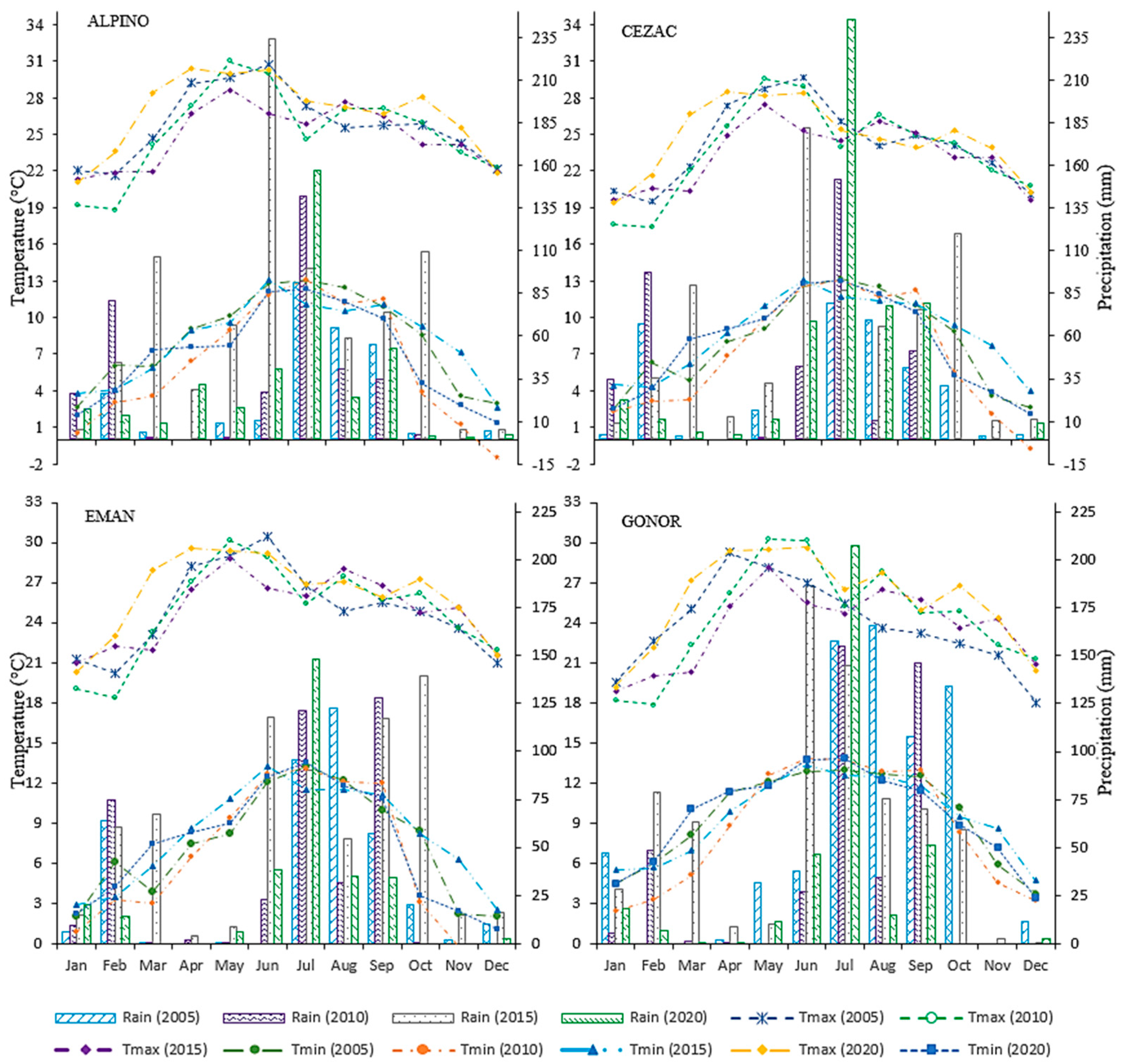
3.1. Climatic Conditions

Precipitation was one of the climatic variables with the greatest variation at the four stations, with minimum and maximum values of 268 mm and 838.4 mm in the 2005 and 2015 cycles, respectively, for the ALPINO station (Figure 1). Maximum temperatures were recorded between April and June. The extreme average maximum temperature occurred at the ALPINO station in May 2010 with 31.0 °C. Minimum temperatures were recorded in December and January, with an average minimum value of −1.8 °C at the EMAN station in December 2010. The maximum radiation was recorded at the GONOR station with 34.4 (MJ m⁻²day⁻¹) in May 2010. Finally, the maximum reference evapotranspiration of 7.2 mm occurred in May 2010 and April 2020 at the CEZAC station (Figure 1).

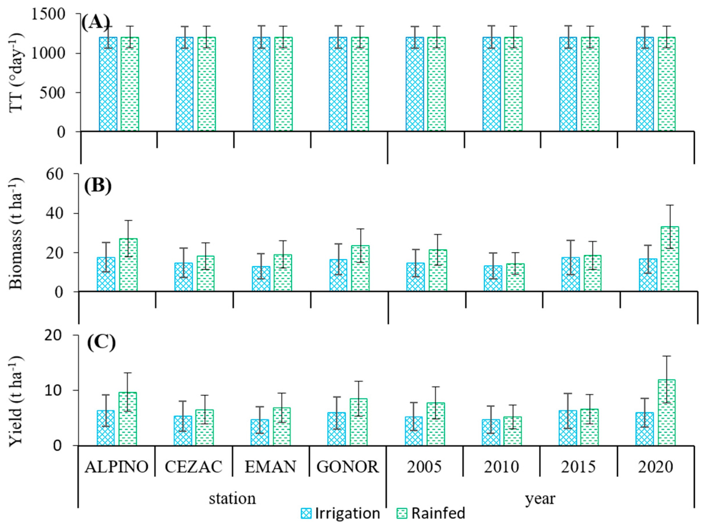
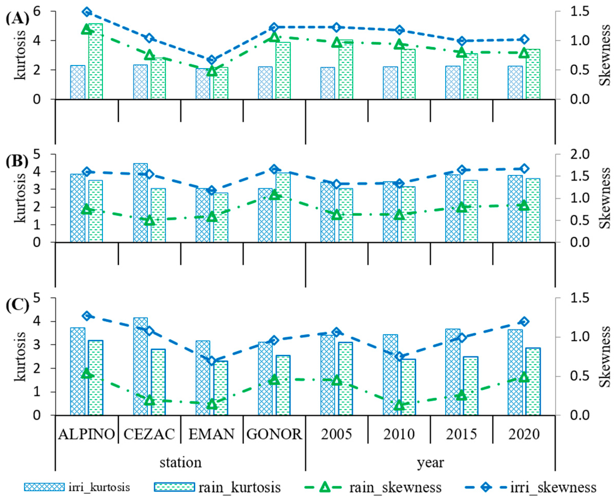
3.2. Uncertainty Analysis

Thermal time was statistically equal (p < 0.01) for the irrigated and rainfed conditions with an overall average of 1204.8 ± 0.47 °C day⁻¹. Bio and Y were 29.4% higher for the rainfed than irrigated condition. The averages for both management systems (irrigated and rainfed) used at the stations with respect to the years were similar; however, the standard deviation was higher in years with 56%, 39% and 38% for TT, Bio and Y, respectively; that is, there was greater dispersion of data in space, indicating greater spatial variability.

In Bio for the irrigated condition, the range was from 11.96 to 22.33 t ha⁻¹, whereas in the rainfed condition it was from 6.90 to 34.11 t ha⁻¹. For Y it was from 4.31 to 8.03 t ha⁻¹ and 2.48 to 12.29 t ha⁻¹ for the irrigated and rainfed conditions, respectively. The high dispersion of the rainfed data for this variable can be mainly attributed to the low temperatures recorded during the simulation, which caused an increase of up to 110 days compared to the simulations for the irrigated condition. For the TT variable, the coefficients of variation were the lowest at 11.49% and 11.47% for irrigated and rainfed beans, respectively. The corresponding values for Y, in that same order, were the highest at 49.52% and 39.71%. However, the average coefficient of variation of the three variables was 36.32% and 29.67% for irrigated and rainfed beans, respectively (Figure 2).

The average kurtoses for TT, Bio and Y for irrigated beans were, respectively, 1.8 ± 0.001, 4.4 ± 0.3 and 4.8 ± 0.3, while for rainfed beans they were, respectively, 1.8 ± 0.001, 3.8 ± 0.2 and 4.2 ± 0.2. These values indicate that TT presents a higher concentration of the data above the mean, and the lowest concentration above the mean is observed in Y. The average kurtoses for years and stations are equal, which indicates a good robustness of the model to spatial and temporal change in the input variables (Figure 3).

Skewness values close to zero and high variance values show that TT fits a uniform distribution, for Bio and Y the overall averages were 0.9 and 1.0, respectively. According to the observed values, the distributions of the output variable for stations and years have positive skewness; that is, they are skewed to the right (Figure 3). This implies that the model’s output variables do not fit a normal distribution.

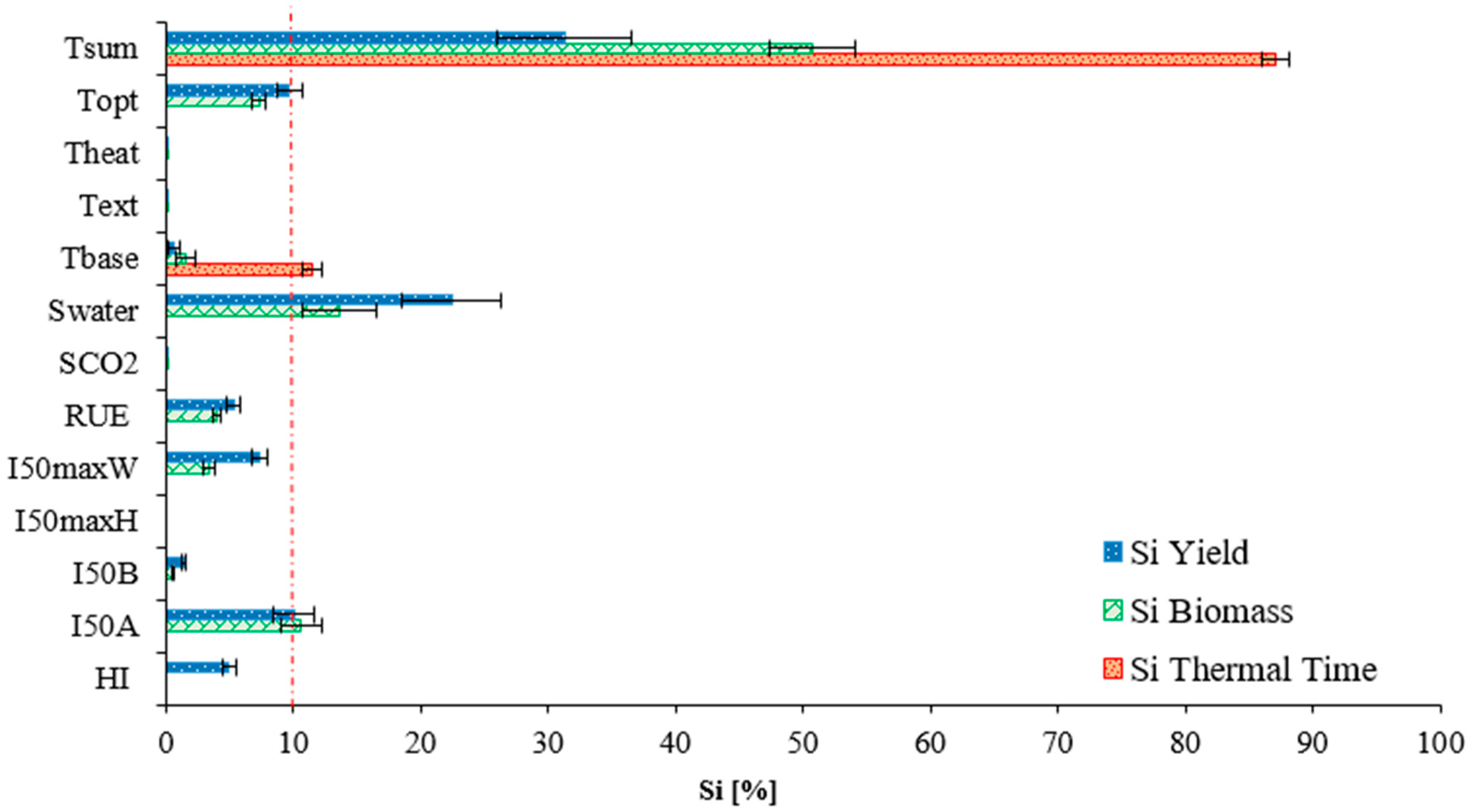
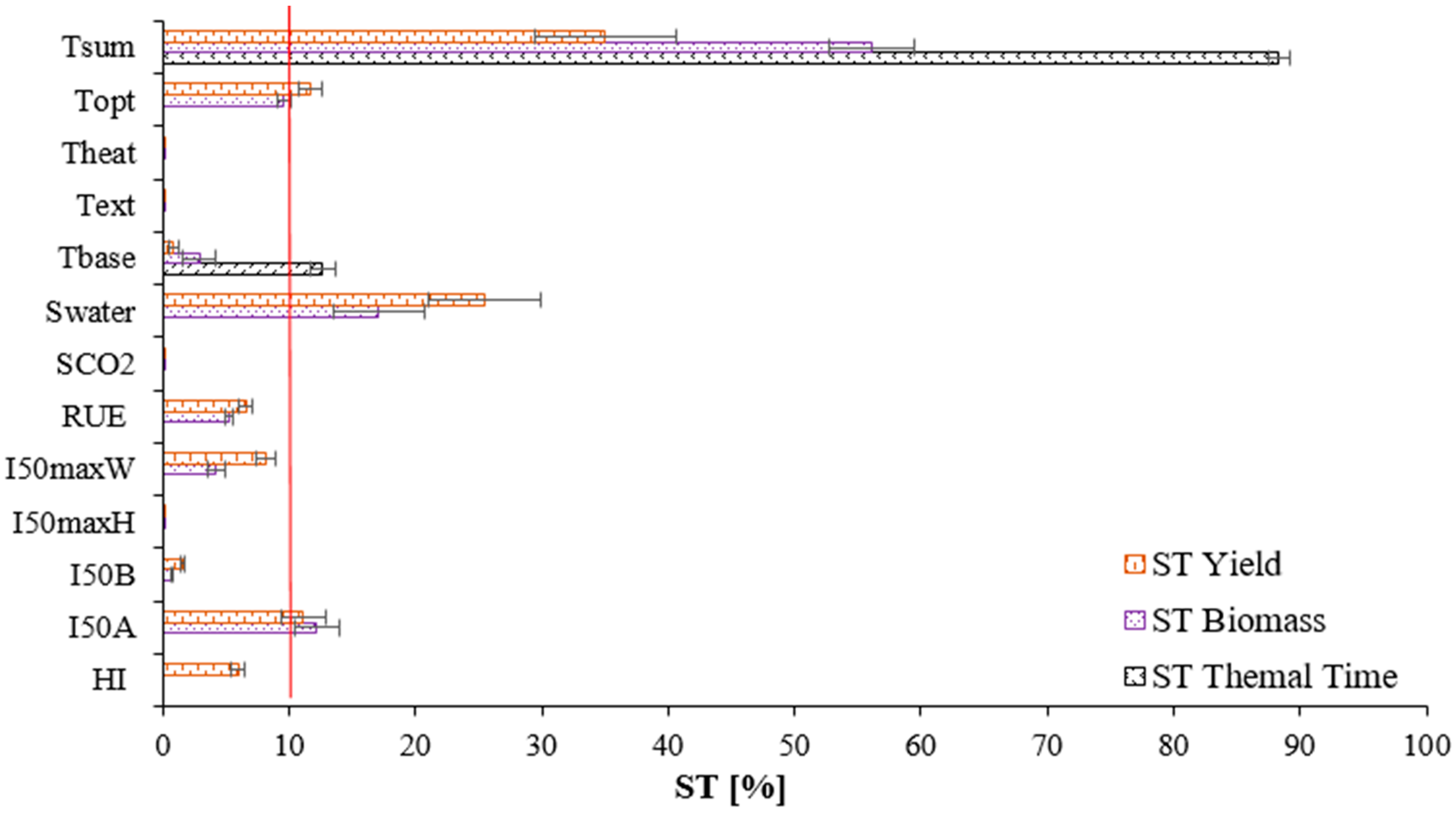
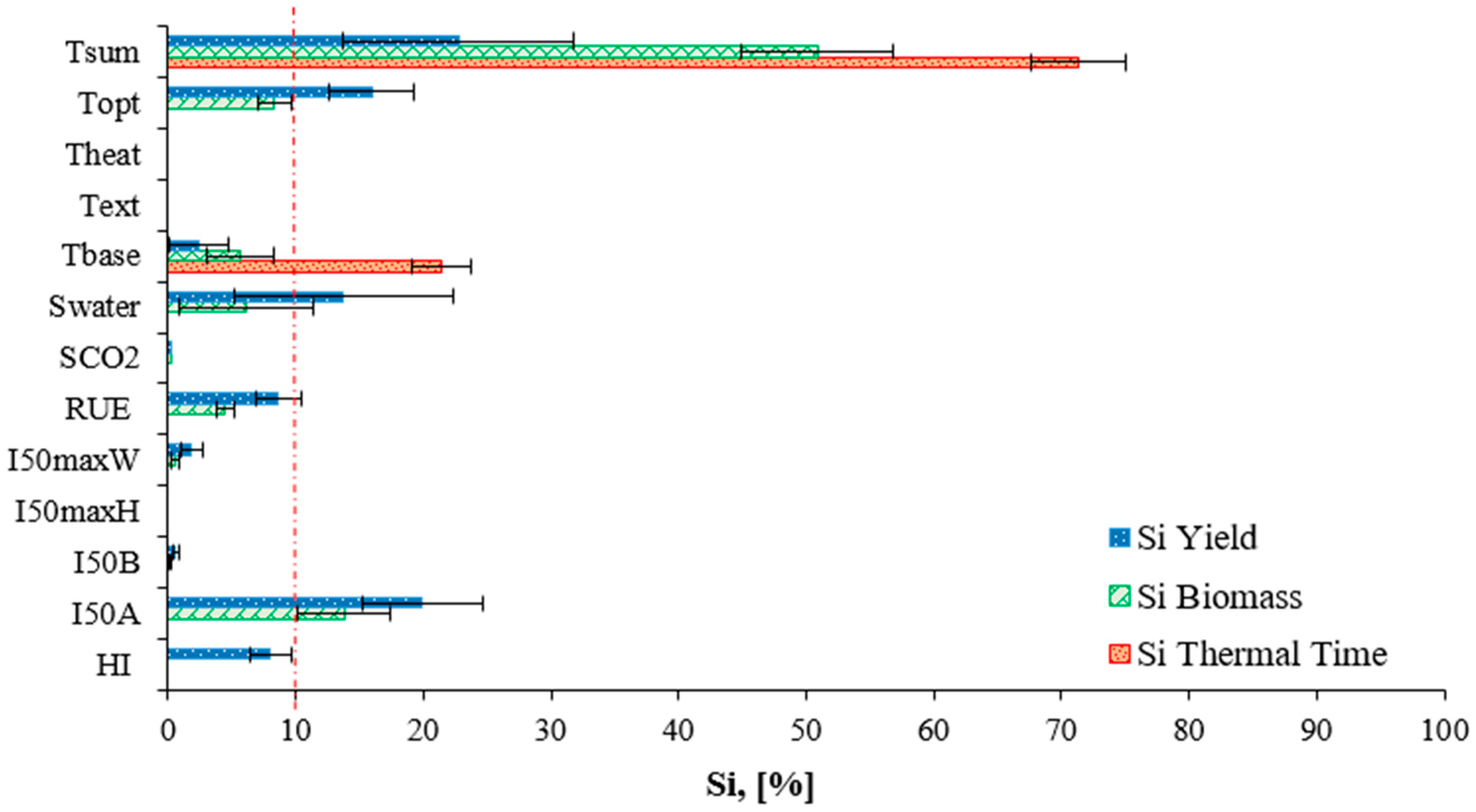
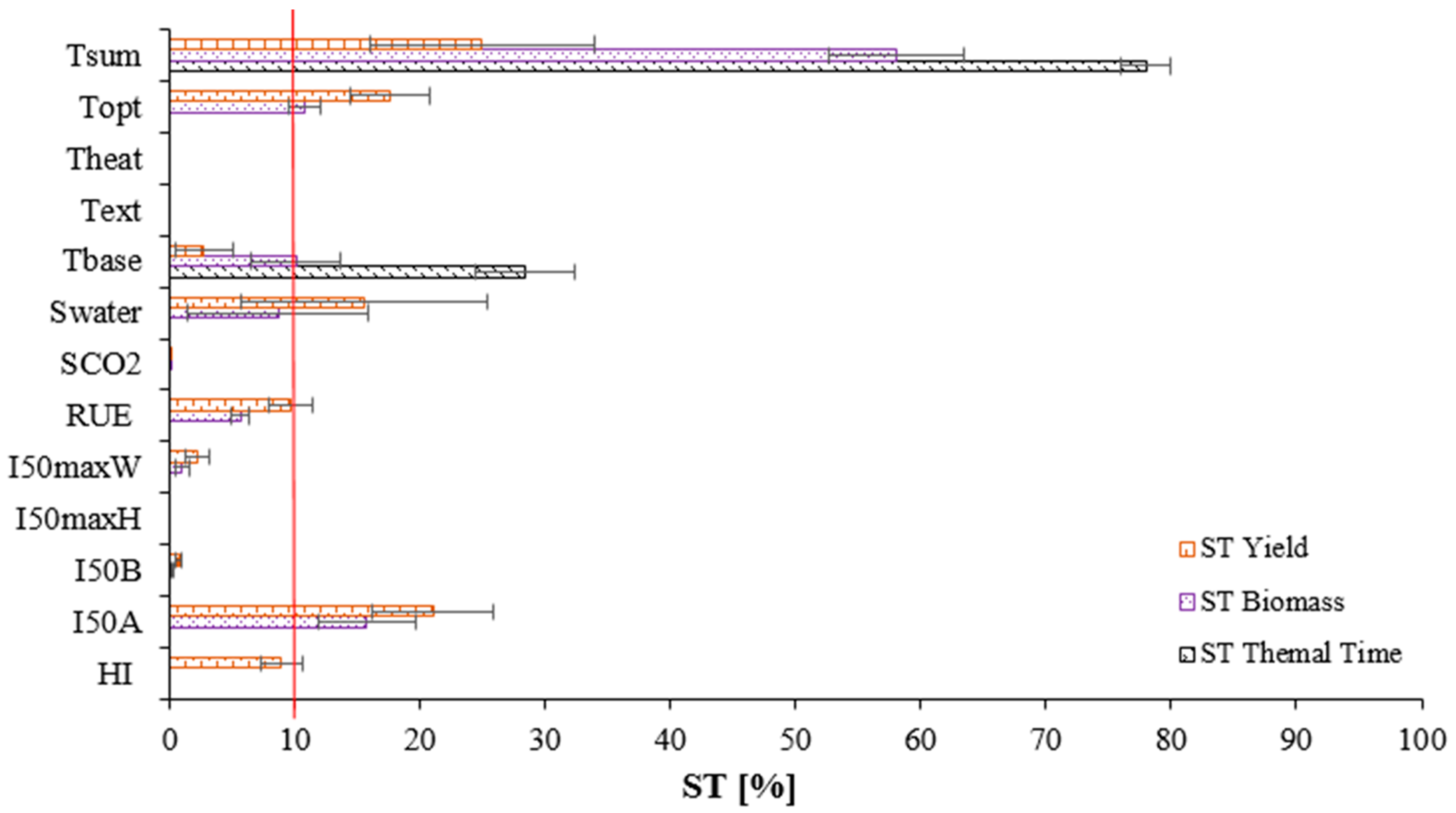
3.3. Sensitivity Analysis

The first order indices (S_i) were 7.70%, 16.64% and 10.88% lower than the total effect indices (S_Ti) for TT, Bio and Y, respectively (Figure 4 and Figure 5), indicating interaction between parameters. S_i and S_Ti were similar when averaged across stations and years for both bean production systems; that is, the input variables for time and space had the same effect on the parameters.

When averaging the indices by management system, it was observed that under the irrigated condition, the most influential parameters for TT, Bio and Y were: Tsum, Swater, Tbase, Topt and I50A in order of influence. The highest standard deviation was observed in TT for the Tsum parameter with a maximum S_Ti of 46.22 (CEZAC 2015) and a minimum of 28.28 (EMAN 2020), and in the Swater parameter with 30.04 and 15.58 for EMAN 2005 and ALPINO 2015, respectively (Figure 4 and Figure 5). For CEZAC 2015 the average simulation was 121 days and for EMAN 2020 it was 108 days. On the other hand, for CEZAC 2015, average Tmax and Tmin values of 25.69 and 11.53 °C were observed, and of 28.81 and 11.21 °C for EMAN, respectively. For EMAN 2005 and ALPINO 2015, during the simulation, the effective precipitation values were 139.50 mm and 340.30 mm, respectively.

In the rainfed condition the most influential parameters were: Tsum, Tbase, I50A, Topt, Swater and RUE (Figure 6 and Figure 7). Parameter I50A was the most influential parameter, Swater was less important and RUE was considered an influential parameter with respect to irrigation. I50A presented a maximum S_Ti of 29.4 (ALPINO 2010) and a minimum of 11.11 (GONOR 2005). The average simulations were 171.5 and 169.5 days for ALPINO 2010 and GONOR 2005, respectively; both scenarios presented a similar average temperature during the simulation. However, at the ALPINO station in 2010, precipitation (Pp) of 219.6 mm, mean solar radiation (Rs) of 59.24 MJ m⁻² day⁻¹ and mean reference evapotranspiration (ETo) of 3.85 mm day⁻¹ were recorded. At the GONOR station in 2005 during the simulation, a Pp of 570.4 mm, Rs of 65.77 MJ m⁻² day⁻¹ and an ETo of 4.95 mm day⁻¹ were recorded.

For Swater, an S_Ti range from 3.27 to 43.30 was observed at the CEZAC station in 2020 and 2010, respectively, suggesting that the temporal variation at this station affected the influence of Swater on the model variables. At the CEZAC 2020 station, during the simulation, the following values were recorded: Tmax = 24.13 °C, Tmin = 8.29 °C, Pp = 405 mm, Rs = 69.28 MJm⁻² day⁻¹ and Eto = 4.35 mm day⁻¹. At this same station, but in 2010, the values were: Tmax = 23.99 °C, Tmin = 7.68 °C, Pp = 214 mm, Rs = 70.61 MJ m⁻² day⁻¹ and Eto = 4.54 mm day⁻¹.

The RUE parameter is directly related to Rs. During the simulation, Rs in the irrigated condition was 21.1% higher relative to the rainfed condition. In RUE, the maximum and minimum S_Ti were 12.73 (CEZAC 2020) and 5.74 (CEZAC 2010), respectively. The CEZAC station in 2020 exceeded the precipitation of the station’s 2010 amount by 47.16% and its Tmin by 7.37%, but it was lower by 1.9% and 4.48% for Rs and ETo, respectively. In addition, at CEZAC in 2010 the simulation was 271 days and 258 days in 2020 with a Tsum of 1440 °C day⁻¹; this difference of 35 simulation days is attributable to the Tmin of 2.05 and −0.72 °C at CEZAC 2010 for November and December, respectively. However, the influence of RUE is related to the variation in Rs of those last 35 days of simulation where CEZAC in 2010 was 11.67% higher than CEZAC in 2020.

4. Discussion

4.1. Climatic Conditions

The climate of the four study regions is dry and semi-dry [46], classified as cold semi-arid (Bsk) according to Koppen as modified by García [47], with average annual precipitation of 400 mm that occurs mainly in the summer and early fall. However, precipitation shows considerable temporal and spatial variability, which affects agricultural production, mainly of the rainfed system [48,49], and induces a reduction in bean production in the temperate semi-arid highlands of north-central Mexico [50]. On the other hand, the minimum temperature in October and November in most scenarios was lower than the Tbase (8 °C) for beans [43]. The latter has a greater effect on rainfed simulations for Tsum greater than 1200 °C d⁻¹; Tbase is of great importance for the calculation of TT [51] and influences plant processes and development [52].

4.2. Uncertainty Analysis

The final value of the simulation in the output variable reliably describes the output response of the dynamic models used by Guo et al. [25] and can be used to compare the simulation in irrigated and rainfed conditions. Tigkas et al. [53] point out that drought has significant effects on the agricultural sector. That is, agricultural production is sensitive to the spatial and temporal distribution of precipitation [54]. On the other hand, the simulated yields in the irrigated scenarios are within those reported by Kader et al. [55], of 4.0 and 6.0 t ha⁻¹, whereas Baez-Gonzalez et al. [43] report yields of 1.8 t ha⁻¹ under rainfed conditions for common bean cv “Pinto Saltillo;” however, the SIMPLE model overestimates yields, attributable to the low temperatures during the simulation and the uncertainty applied to the Tsum parameter, which generates long crop cycles, even outside the limit of the onset of frost in the region. In addition, Acosta-Gallegos and White [56] and Yan and Wallace [57] state that temperature and photoperiod modify the growth and development stages of the bean crop. For these reasons, special care should be taken with the Tsum parameter, and equations representing the effect of the photoperiod on bean yield should be incorporated into the model structure.

According to the coefficient of variation, the variable least sensitive to the 10% uncertainty of the parameters was TT, while Bio was the most sensitive. CV values < 30% mean a low dispersion of the data over the mean of the output variables; that is, it tends to homogeneity. The SIMPLE model can be reliable and robust by reducing the uncertainty of the most influential parameters to represent biomass production in Zacatecas. Martínez-Ruiz et al. [58] carried out an SA of the HORTSYST model and reported that by decreasing the uncertainty of the parameters, lower coefficient of variation values are observed.

The kurtosis and skewness values show a concentration of the data to the left; that is, low values are more frequent and show a positive bias for Bio and Y. Moreover, the results show the possibility of rejecting the assumption of normality [59,60]. However, Harri et al. [61] point out that crop yields can be fitted to different distributions (beta, gamma, hyperbolic tangent function transformation, logistic, lognormal and Weibull) and not necessarily to a normal distribution.

The results from the UA are a starting point to explore other limits or other probability density functions for the parameters, considering the physical and biological boundaries, due to the stochastic nature of processes involved in growth and crop development. Overall uncertainty analysis results increase the reliability of the SIMPLE model applied to common beans grown in semi-arid lands (Figure 2 and Figure 3).

4.3. Sensitivity Analysis

Several authors agree that the interaction of the parameters exerts influence on the variables predicted by a mathematical model [21,58]. Therefore, the total effect indices are the values indicated to determine the influence of the parameters on the model outputs. This result supports the findings of Krishnan et al. [18], who studied the influence of the parameters in the InfoCrop model under contrasting conditions and found no evidence that agro-climatic conditions and year had an influence on the ranking of candidate parameters for calibration. In this study, soil water availability related to management strongly affected the ranking of the most influential parameters of the SIMPLE model.

The Tsum parameter is related to the length of the growth period, and for the SIMPLE model it determines the end of the simulation. This variable has a great influence on thermal time (TT), biomass (Bio) and yield (Y). However, in contrast to the above, Ratjen et al. [62] state that thermal time cannot fully capture the allometric relationship between leaf area index and the biomass of maize and wheat. TT measures the time of phenological stage change and is highly dependent on temperature. The uniform distribution of TT in this study reflects the distribution applied in Tsum. For this reason, great care should be taken in selecting the uncertainty and distribution used in the model parameters to avoid erroneous inferences on their influence. Jin et al. [63] note that flat distributions indicate that the model parameters that generate them are uncertain.

Tbase is of great importance in the calculation of TT [51]. Barrio-Gomez et al. [64] note that the optimal Tbase for the different bean varieties planted in Mexico is from 8.2 to 8.4 °C. It is observed that on 1 June (start of simulation for the rainfed condition), Tmax and Tmin begin to decrease and Tbase has a greater influence on the simulation of bean growth and development with the SIMPLE model and has greater importance with respect to irrigation (15 April, start of simulation).

On the other hand, the Swater parameter relates to water availability and its effect on biomass production [25]. Beebe et al. [65] note that the irrigation sheet (Lr) for bean production is from 300 to 500 mm. This indicates that sheets close to these values would have lower Swater S_Ti values. However, at the EMAN station in 2005, maximum values of 427.2 mm and 139.5 mm were recorded, and at the ALPINO station in 2015, 202.3 and 340.3 mm of Lr and Pe, respectively, were recorded. Effective precipitation has a greater influence on the Swater parameter than that of water stored in the soil (Lr plus Pe). Pp is the input variable with the greatest effect on Swater due to its stochastic distribution in time and space. Precipitation is the climatic variable with the greatest spatiotemporal uncertainty in spring–summer for arid and semi-arid climates. The most important variations were for irrigated (spring) and rainfed (summer) conditions, which influenced the indices. However, there was no wide variation in parameters observed with respect to the spatial analysis (stations) and temporal analysis (years), so the SIMPLE model is very robust for simulating irrigated and rainfed beans in Zacatecas. For rainfed beans, August precipitation has the greatest effect on the influence of Swater on Bio and Y. Osuna-Ceja et al. [66] point out that the amount and distribution of precipitation affects the yield of “Pinto Saltillo” beans under semi-arid conditions in northern Mexico. On the other hand, Padilla et al. [67] state that the accumulated precipitation during the reproductive stage is a determining factor for bean yield under rainfed conditions; the month of August coincides with this stage, where the crop is more sensitive to water stress [68,69]. For the SIMPLE model, being a model based on radiation interception, I50 A was expected to be an influential parameter for irrigated and rainfed bean cultivation as it defines the radiation interception curve from planting to physiological maturity [25]. Furthermore, photosynthetically active radiation is highly associated with biomass production [70]. For the rainfed condition, radiation was lower, so the RUE parameter takes on importance.

The global sensitivity analysis carried out (Figure 4, Figure 5, Figure 6 and Figure 7) allows determination of the most influential parameters of the SIMPLE model; therefore, the parameters Tsum, Swater, Tbase, I50 A and Topt need to be estimated by carrying out a model calibration to apply the SIMPLE model in or as a decision support system.

5. Conclusions

The uncertainties of the output variables are related to precipitation, which greatly influenced the SIMPLE model simulation, followed by temperature and solar radiation. It is advisable to perform an uncertainty analysis of the input variables to make a better inference about the sources of uncertainty and model performance. Moreover, to improve the robustness and quality of the prediction for both irrigated and rainfed beans, it is necessary to pay special attention to the Tsum parameter. Therefore, it is suggested to apply a small uncertainty (>10%) or to use a normal distribution when calibrating the parameters. On the other hand, it is necessary to obtain the intersection curve to find, from the experimental data, the parameters I50 A and I50 B for each variety.

According to the global sensitivity analysis, the SIMPLE crop model with climatic data from Zacatecas in spring (irrigated condition) suggests five influential parameters. Tsum is the index that most affects the system for the simulation of thermal time, biomass and yield, and Swater is the most important in the irrigated condition, followed by I50A, then Tbase and Topt. For winter (rainfed condition) it is important to consider RUE, giving a total of six more influential parameters to represent the climatic conditions of the four bean-producing regions of Zacatecas.

References

1. Hayat, I.; Ahmad, A.; Masud, T.; Ahmed, A.; Bashir, S. Nutritional and health perspectives of beans (Phaseolus vulgaris L.): An overview. Crit. Rev. Food Sci. Nutr. 2014, 54, 580–592. [Google Scholar] [CrossRef] [PubMed]
2. Centro de Estudios para el Desarrollo Rural Sustentable y la Soberanía Alimentaria (CEDRSSA). Mercado del Frijol, Situación y Prospectiva. 2020. Available online: http://www.cedrssa.gob.mx/files/b/13/53Mercado%20del%20frijol.pdf (accessed on 15 April 2022).
3. Servicio de Información y Estadística Agroalimentaria y Pesquera Información Agrícola (SIAP). Avances Mensuales por Estado. Estadisticas 2010–2010. 2021. Available online: https://www.siap.sagarpa.gob.mx (accessed on 15 May 2021).
4. van Ittersum, M.K.; Leffelaar, P.A.; van Keulen, H.; Kropff, M.J.; Bastiaans, L.; Goudriaan, J. On approaches and applications of the Wageningen crop models. Eur. J. Agron. 2003, 18, 201–234. [Google Scholar] [CrossRef]
5. Thornley, J.H.; France, J. Mathematical Models in Agriculture: Quantitative Methods for the Plant, Animal and Ecological Sciences; Cabi: Wallingford, UK, 2007. [Google Scholar] [CrossRef]
6. Lopez-Cruz, I.L.; Ramírez-Arias, A.; Rojano-Aguilar, A. Modelos matemáticos de hortalizas en invernadero: Trascendiendo la contemplación de la dinámica de cultivos. Rev. Chapingo Ser. Hortic. 2005, 11, 257–267. Available online: https://www.redalyc.org/articulo.oa?id=60911211 (accessed on 28 June 2022). [CrossRef]
7. Keating, B.A.; Thorburn, P.J. Modelling crops and cropping systems—Evolving purpose, practice and prospects. Eur. J. Agron. 2018, 100, 163–176. [Google Scholar] [CrossRef]
8. Ljung, L.; Glad, T. Modeling of Dynamic Systems; PTR Prentice Hall: Englewood Cliffs, NJ, USA, 1994. [Google Scholar]
9. Voinov, A.A. Systems Science and Modeling for Ecological Economics; Academic Press: Cambridge, MA, USA, 2010; Available online: https://ezproxy2.utwente.nl/login?url=http://www.dawsonera.com/depp/reader/protected/external/AbstractView/S9780080886176 (accessed on 28 June 2022).
10. Wallach, D.; Makowski, D.; Jones, J.W.; Brun, F. Working with Dynamic Crop Models: Methods, Tools and Examples for Agriculture and Environment; Academic Press: Cambridge, MA, USA, 2019. [Google Scholar]
11. Saltelli, A.; Ratto, M.; Tarantola, S.; Campolongo, F.; Commission, E. Sensitivity analysis practices: Strategies for model-based inference. Reliab. Eng. Syst. Saf. 2006, 91, 1109–1125. [Google Scholar] [CrossRef]
12. Saltelli, A.; Tarantola, S.; Campolongo, F.; Ratto, M. Sensitivity Analysis in Practice: A Guide to Assessing Scientific Models; Wiley: New York, NY, USA, 2004; Volume 1. [Google Scholar]
13. Coucheney, E.; Buis, S.; Launay, M.; Constantin, J.; Mary, B.; García de Cortázar-Atauri, I.; Léonard, J. Accuracy, robustness and behavior of the STICS soil–crop model for plant, water and nitrogen outputs: Evaluation over a wide range of agro-environmental conditions in France. Environ. Model. Softw. 2015, 64, 177–190. [Google Scholar] [CrossRef]
14. Ceglar, A.; Kajfež-Bogataj, L. Simulation of maize yield in current and changed climatic conditions: Addressing modelling uncertainties and the importance of bias correction in climate model simulations. Eur. J. Agron. 2012, 37, 83–95. [Google Scholar] [CrossRef]
15. Eitzinger, J.; Thaler, S.; Schmid, E.; Strauss, F.; Ferrise, R.; Moriondo, M.; ÇAylak, O. Sensitivities of crop models to extreme weather conditions during flowering period demonstrated for maize and winter wheat in Austria. J. Agric. Sci. 2012, 151, 813–835. [Google Scholar] [CrossRef]
16. Rötter, R.P.; Palosuo, T.; Kersebaum, K.C.; Angulo, C.; Bindi, M.; Ewert, F.; Trnka, M. Simulation of spring barley yield in different climatic zones of Northern and Central Europe: A comparison of nine crop models. Field Crops Res. 2012, 133, 23–36. [Google Scholar] [CrossRef]
17. Fleisher, D.H.; Condori, B.; Quiroz, R.; Alva, A.; Asseng, S.; Barreda, C.; Woli, P. A potato model intercomparison across varying climates and productivity levels. Glob. Chang. Biol. 2017, 23, 1258–1281. [Google Scholar] [CrossRef]
18. Krishnan, P.; Maity, P.P.; Kundu, M. Sensitivity analysis of cultivar parameters to simulate wheat crop growth and yield under moisture and temperature stress conditions. Heliyon 2021, 7, e07602. [Google Scholar] [CrossRef]
19. Dzotsi, K.A.; Basso, B.; Jones, J.W. Development, uncertainty and sensitivity analysis of the simple SALUS crop model in DSSAT. Ecol. Model. 2013, 260, 62–76. [Google Scholar] [CrossRef]
20. Tan, J.; Cui, Y.; Luo, Y. Assessment of uncertainty and sensitivity analyses for ORYZA model under different ranges of parameter variation. Eur. J. Agron. 2017, 91, 54–62. [Google Scholar] [CrossRef]
21. DeJonge, K.C.; Ascough, J.C.; Ahmadi, M.; Andales, A.A.; Arabi, M. Global sensitivity and uncertainty analysis of a dynamic agroecosystem model under different irrigation treatments. Ecol. Model. 2012, 231, 113–125. [Google Scholar] [CrossRef]
22. Silvestro, P.C.; Pignatti, S.; Yang, H.; Yang, G.; Pascucci, S.; Castaldi, F.; Casa, R. Sensitivity analysis of the Aquacrop and SAFYE crop models for the assessment of water limited winter wheat yield in regional scale applications. PLoS ONE 2017, 12, e0187485. [Google Scholar] [CrossRef] [PubMed] [Green Version]
23. Zhao, G.; Bryan, B.A.; Song, X. Sensitivity and uncertainty analysis of the APSIM-wheat model: Interactions between cultivar, environmental, and management parameters. Ecol. Model. 2014, 279, 1–11. [Google Scholar] [CrossRef]
24. Saltelli, A.; Aleksankina, K.; Becker, W.; Fennell, P.; Ferretti, F.; Holst, N.; Wu, Q. Why so many published sensitivity analyses are false: A systematic review of sensitivity analysis practices. Environ. Model. Softw. 2019, 114, 29–39. [Google Scholar] [CrossRef]
25. Zhao, C.; Liu, B.; Xiao, L.; Hoogenboom, G.; Boote, K.J.; Kassie, B.T.; Pavan, W.; Shelia, V.; Kim, K.S.; Hernandez-Ochoa, I.M.; et al. A SIMPLE crop model. Eur. J. Agron. 2019, 104, 97–106. [Google Scholar] [CrossRef]
26. Asseng, S.; Guarin, J.R.; Raman, M.; Monje, O.; Kiss, G.; Despommier, D.D.; Gauthier, P.P.G. Wheat yield potential in controlled-environment vertical farms. Proc. Natl. Acad. Sci. USA 2020, 117, 19131–19135. [Google Scholar] [CrossRef] [PubMed]
27. Li, Y.; Hoogenboom, G.; Asseng, S.; Niu, J.-Y.; Wu, L.; Kang, L.-H. Adaptation of the SIMPLE model to oilseed flax (Linum usitatissimum L.) for arid and semi-arid environments. Agronomy 2022, 12, 1267. [Google Scholar] [CrossRef]
28. Medina, G.G.; Báez, G.A.D.; Ramos, G.J.L. Red de monitoreo agroclimático del estado de Zacatecas. INIFAP, Campo Experimental Zacatecas, México. Despleg. Inf. Núm. 2007, 15, 14. Available online: http://www.zacatecas.inifap.gob.mx/historico.php?id=26786 (accessed on 15 December 2021).
29. Medina-García, G.; Rumayor-Rodríguez, A.F.; Cabañas-Cruz, B.; Luna-Flores, M.; Ruiz-Corral, J.A.; Gallegos-Valdez, C.; Madero-Tamargo, J.; Gutiérrez-Sánchez, J.R.; Rubio-Díaz, S.; Bravo-Lozano, A.G. Potencial productivo de especies agrícolas en el estado de Zacatecas. In Instituto Nacional de Investigaciones Forestales, Agrícolas y Pecuarias; Libro Técnico Núm. 2; Centro de Investigación Regional Norte Centro, Calera de V. R.: Zacatecas, México, 2003; p. 157. Available online: http://zacatecas.inifap.gob.mx/publicaciones/Pot_Prod_de_Especies_Agricolas_en_Zacatecas.pdf (accessed on 28 June 2022).
30. Cid Ríos, J.A.; Hernández, M.R.; Velázquez Valle, R.; Mena Covarrubias, J. Producción de semilla de frijol. In Folleto Técnico No. 63. Campo Experimental Zacatecas; CIRNOC-INIFAP: Calera, Zacatecas, México, 2014; p. 69. Available online: http://zacatecas.inifap.gob.mx/publicaciones/produccionSemillaFrijol.pdf (accessed on 28 June 2022).
31. Servín-Palestina, M.; Tijerina Chávez, L.; Medina García, G.; Palacios Velez, O.; Flores Magdaleno, H. Sistema para programar y calendarizar el riego de los cultivos en tiempo real. Rev. Mex. Cienc. Agríc. 2017, 8, 423–430. [Google Scholar] [CrossRef] [Green Version]
32. Allen, R.G.; Pereira, L.S.; Raes, D.; Smith, M. Evapotranspiración del cultivo: Guía para la determinación de los requerimientos de agua de los cultivos. In Estudio FAO Riego y Drenaje; FAO: Roma, Italy, 2006; pp. 56–323. Available online: http://www.fao.org/docrep/009/x0490s/x0490s00.htm (accessed on 28 June 2022).
33. Monteith, J.L. Light distribution and photosynthesis in field crops. Ann. Bot. 1965, 29, 17–37. [Google Scholar] [CrossRef]
34. Amir, J.; Sinclair, T.R. A model of water limitation on spring wheat growth and yield. Field Crops Res. 1991, 28, 59–69. [Google Scholar] [CrossRef]
35. Woli, P.; Jones, J.; Ingram, K.; Fraisse, C. Agricultural reference index for drought (ARID). Agron. J. 2012, 104, 287–300. [Google Scholar] [CrossRef]
36. Matott, L.S.; Babendreier, J.E.; Purucker, S.T. Evaluating uncertainty in integrated environmental models: A review of concepts and tools. Water Resour. Res. 2009, 45, 1–14. [Google Scholar] [CrossRef] [Green Version]
37. Monod, H.; Naud, C.; Makowski, D. Uncertainty and sensitivity analysis for crop models. In Working with Dynamic Crop Models, Chapter 3; Elsevier: Amsterdam, The Netherlands, 2006; pp. 55–100. ISBN 0-444-52135-6. Available online: https://hal.inrae.fr/hal-02823185 (accessed on 28 June 2022).
38. Walters, R.W.; Huyse, L. Uncertainty analysis for fluid mechanics with applications. In ICASE Report No. 2002-1 NASA/CR-2002-211449; ICASE: Fort Belvoir, VA, USA, 2002; Available online: https://apps.dtic.mil/sti/citations/ADA401486 (accessed on 28 June 2022).
39. Baez-Gonzalez, A.D.; Fajardo-Díaz, R.; Garcia-Romero, G.; Osuna-Ceja, E.; Kiniry, J.R.; Meki, M.N. High sowing densities in rainfed common beans (Phaseolus vulgaris L.) in Mexican semi-arid highlands under future climate change. Agronomy 2020, 10, 442. [Google Scholar] [CrossRef] [Green Version]
40. Karimzadeh Soureshjani, H.; Nezami, A.; Kafi, M.; Tadayon, M. Responses of two common bean (Phaseolus vulgaris L.) genotypes to deficit irrigation. Agric. Water Manag. 2019, 213, 270–279. [Google Scholar] [CrossRef]
41. Omae, H.; Kumar, A.; Shono, M. Adaptation to high temperature and water deficit in the common bean (Phaseolus vulgaris L.) during the reproductive period. J. Bot. 2012, 2012, 803413. [Google Scholar] [CrossRef] [Green Version]
42. Sobol, I.M. On sensitivity estimates for nonlinear mathematical models. Mat. Model. 1990, 2, 112–118. Available online: http://mi.mathnet.ru/eng/mm/v2/i1/p112 (accessed on 22 February 2022).
43. Saltelli, A.; Ratto, M.; Andres, T.; Campolongo, F.; Cariboni, J.; Gatelli, D.; Tarantola, S. Global Sensitivity Analysis: The Primer; John Wiley & Sons: Hoboken, NJ, USA, 2008. [Google Scholar] [CrossRef] [Green Version]
44. Jansen, M.J. Analysis of variance designs for model output. Comput. Phys. Commun. 1999, 117, 35–43. [Google Scholar] [CrossRef]
45. Saltelli, A.; Annoni, P.; Azzini, I.; Campolongo, F.; Ratto, M.; Tarantola, S. Variance based sensitivity analysis of model output. Design and estimator for the total sensitivity index. Comput. Phys. Commun. 2010, 181, 259–270. [Google Scholar] [CrossRef]
46. INEGI (Instituto Nacional de Estadística y Geografía). Cuéntame de México: Clima de Zacatecas. Instituto Nacional de Estadística y Geografía. 2015. Available online: https://cuentame.inegi.org.mx/monografias/informacion/zac/territorio/clima.aspx?tema=me&e=32 (accessed on 28 June 2022).
47. García, E. Distribución de la precipitación en la República Mexicana. Investig. Geogr. 1974, 1, 7–20. [Google Scholar] [CrossRef]
48. Esquivel-Arriaga, G.; Sánchez-Cohen, I.; López-Santos, A.; Velásquez-Valle, M.A.; Bueno-Hurtado, P. Enfoque metodológico para cuantificar el efecto del cambio en patrones de clima sobre el rendimiento del cultivo de frijol en el estado de Durango. Rev. Chapingo Ser. Zonas Áridas 2016, 15, 17–28. [Google Scholar] [CrossRef] [Green Version]
49. Rosenzweig, C. Climate Change & Agriculture. Learning Lessons & Proposing Solutions; Iowa State University: Ames, IA, USA, 2007; p. 28. [Google Scholar]
50. Osuna-Ceja, E.S.; Figueroa-Sandoval, B.; Martínez-Gamiño, M.Á.; Pimentel-López, J. Un sistema agroforestal de secano para el altiplano semiárido de México. Rev. Mex. Cienc. Agríc. 2019, 10, 89–103. [Google Scholar] [CrossRef] [Green Version]
51. Masle, J.; Doussinault, G.; Farquhar, G.D.; Sun, B. Foliar stage in wheat correlates better to photothermal time than to thermal time. Plant Cell Environ. 1989, 12, 235–247. [Google Scholar] [CrossRef]
52. Neto, N.B.M.; Prioli, M.R.; Gatti, A.B.; Cardoso, V.J.M. Temperature effects on seed germination in races of common beans (Phaseolus vulgaris L.). Acta Sci. Agron. 2006, 28, 155–164. Available online: https://www.redalyc.org/articulo.oa?id=303026569012 (accessed on 28 June 2022).
53. Tigkas, D.; Vangelis, H.; Tsakiris, G. Drought characterisation based on an agriculture-oriented standardised precipitation index. Theor. Appl. Climatol. 2019, 135, 1435–1447. [Google Scholar] [CrossRef]
54. Lausier, A.M.; Jain, S. Overlooked trends in observed global annual precipitation reveal underestimated risks. Sci. Rep. 2018, 8, 16746. [Google Scholar] [CrossRef] [Green Version]
55. Kader, K.A.; Balasubramanian, P.M.; Chatterton, S. Influence of irrigation and plant canopy architecture on white mould disease of dry bean. Can. J. Plant Sci. 2018, 98, 1280–1292. [Google Scholar] [CrossRef]
56. Acosta-Gallegos, J.A.; White, J.W. Phenological plasticity as an adaptation by common bean to rainfed environments. Crop Sci. 1995, 35, 199–204. [Google Scholar] [CrossRef]
57. Yan, W.; Wallace, D.H. Simulation and prediction of plant phenology for five crops based on photoperiod temperature interaction. Ann. Bot. 1998, 81, 705–716. [Google Scholar] [CrossRef] [Green Version]
58. Martínez-Ruiz, A.; Ruiz-García, A.; Prado-Hernández, J.V.; López-Cruz, I.L.; Valencia-Islas, J.O.; Pineda-Pineda, J. Global sensitivity analysis and calibration by differential evolution algorithm of HORTSYST crop model for fertigation management. Water 2021, 13, 610. [Google Scholar] [CrossRef]
59. Patel, J.K.; Read, C.B. Handbook of the Normal Distribution; CRC Press: Boca Raton, FL, USA, 1996; Volume 150. [Google Scholar]
60. Joanes, D.N.; Gill, C.A. Comparing measures of sample skewness and kurtosis. J. R. Stat. Soc. Ser. D 1998, 47, 183–189. [Google Scholar] [CrossRef]
61. Harri, A.; Erdem, C.; Coble, K.H.; Knight, T.O. Crop yield distributions: A reconciliation of previous research and statistical tests for normality. Appl. Econ. Perspect. Policy 2009, 31, 163–182. [Google Scholar] [CrossRef]
62. Ratjen, A.M.; Lemaire, G.; Kage, H.; Plénet, D.; Justes, E. Key variables for simulating leaf area and N status: Biomass based relations versus phenology driven approaches. Eur. J. Agron. 2018, 100, 110–117. [Google Scholar] [CrossRef]
63. Jin, X.; Xu, C.Y.; Zhang, Q.; Singh, V.P. Parameter and modeling uncertainty simulated by GLUE and a formal Bayesian method for a conceptual hydrological model. J. Hydrol. 2010, 383, 147–155. [Google Scholar] [CrossRef]
64. Barrios-Gómez, E.J.; López-Castañeda, C. Temperatura base y tasa de extensión foliar en frijol. Agrociencia 2009, 43, 29–35. Available online: http://www.scielo.org.mx/scielo.php?pid=S1405-31952009000100004&script=sci_abstract&tlng=pt (accessed on 28 June 2022).
65. Beebe, S.; Ramirez, J.; Jarvis, A.; Rao, I.M.; Mosquera, G.; Bueno, J.M.; Blair, M.W. Genetic improvement of common beans and the challenges of climate change. In Crop Adaptation to Climate Change; John Wiley & Sons, Inc.: Hoboken, NJ, USA, 2011; pp. 356–369. [Google Scholar] [CrossRef]
66. Osuna-Ceja, E.S.; Reyes-Muro, L.; Padilla-Ramírez, J.S.; Martínez-Gamiño, M.Á. Rendimiento de frijol Pinto Saltillo en altas densidades de población bajo temporal. Rev. Mex. Cienc. Agríc. 2012, 3, 1389–1400. Available online: http://www.scielo.org.mx/pdf/remexca/v3n7/v3n7a8.pdf (accessed on 28 June 2022).
67. Padilla-Ramírez, J.S.; Ochoa-Márquez, R.; Acosta-Díaz, E.; Acosta-Gallegos, J.A.; Mayek-Pérez, N.; Kelly, J.D. Grain yield of early and late dry bean genotypes under rainfed conditions in Aguascalientes, Mexico. Ann. Rep. Bean Improv. Coop. 2003, 46, 89–90. Available online: https://handle.nal.usda.gov/10113/IND43757200 (accessed on 28 June 2022).
68. Lang, M.; Lichtenthaler, H.K.; Sowinska, M.; Heisel, F.; Miehé, J. Fluorescence imaging of water and temperature stress in plant leaves. J. Plant Physiol. 1996, 148, 613–621. [Google Scholar] [CrossRef]
69. Gallegos, J.A.A.; Shibata, J.K. Effect of water stress on growth and yield of indeterminate dry-bean (Phaseolus vulgaris) cultivars. Field Crops Res. 1989, 20, 81–93. [Google Scholar] [CrossRef]
70. Tesfaye, K.; Walker, S.; Tsubo, M. Radiation interception and radiation use efficiency of three grain legumes under water deficit conditions in a semi-arid environment. Eur. J. Agron. 2006, 25, 60–70. [Google Scholar] [CrossRef]
Figure 1. Climatic conditions of the four stations for the years 2005, 2010, 2015 and 2020.
Agronomy 12 01813 g001
Figure 2. Averages (± standard deviation) of the output variables, thermal time (A), biomass (B) and yield (C) of irrigated and rainfed beans for the SIMPLE model in trials between weather stations and between years in Zacatecas, Mexico.
Agronomy 12 01813 g002
Figure 3. Kurtosis (bars) and skewness (lines) of the output variables: (A) thermal time, (B) biomass and (C) yield of the SIMPLE model in trials between weather stations and between bean production years in Zacatecas, Mexico.
Agronomy 12 01813 g003
Figure 4. First order sensitivity indices (±standard deviation) with Sobol’s method for the irrigated bean crop for the variables predicted by the SIMPLE model; dashed line denotes a 10% threshold.
Agronomy 12 01813 g004
Figure 5. Total effect sensitivity indices (±standard deviation) with Sobol’s method for the irrigated bean crop for the variables predicted by the SIMPLE model; dotted line denotes a threshold of 10%.
Agronomy 12 01813 g005
Figure 6. First order sensitivity indices (±standard deviation) with Sobol’s method for the rainfed bean crop for the variables predicted by the SIMPLE model; dashed line denotes 10% threshold.
Agronomy 12 01813 g006
Figure 7. Total effect sensitivity indices (±standard deviation) with Sobol’s method for the irrigated bean crop for the variables predicted by the SIMPLE model; dashed line denotes a 10% threshold.
Agronomy 12 01813 g007
Publisher’s Note: MDPI stays neutral with regard to jurisdictional claims in published maps and institutional affiliations.