Prediction of Water Stress Episodes in Fruit Trees Based on Soil and Weather Time Series Data

Abstract

Water is a limited resource in arid and semi-arid regions, as is the case in the Mediterranean Basin, where demographic and climatic conditions make it ideal for growing fruits and vegetables, but a greater volume of water is required. Deficit irrigation strategies have proven to be successful in optimizing available water without pernicious impact on yield and harvest quality, but it is essential to control the water stress of the crop. The direct measurement of crop water status is currently performed using midday stem water potential, which is costly in terms of time and labor; therefore, indirect methods are needed for automatic monitoring of crop water stress. In this study, we present a novel approach to indirectly estimate the water stress of 15-year-old mature sweet cherry trees from a time series of soil water status and meteorological variables by using Machine Learning methods (Random Forest and Support Vector Machine). Time information was accounted for by integrating soil and meteorological measurements within arbitrary periods of 3, 6 and 10 days. Supervised binary classification and regression approaches were applied. The binary classification approach allowed for the definition of a model that alerts the farmer when a dangerous crop water stress episode is about to happen a day in advance. Performance metrics F2 and recall of up to 0.735 and 0.769, respectively, were obtained. With the regression approach a R² of up to 0.817 was achieved.

1. Introduction

Water scarcity is a generalized issue that becomes particularly acute under arid and semi-arid climate conditions. The FAO (Food and Agriculture Organization of the United Nations) report “Climate Smart Agriculture Sourcebook” [1] estimates a world population increase of 30% (an increase of two billion people) by 2050, which will require a 60% increase in agricultural production to meet the growing demand for food and to establish certain food security. This increase in agricultural food production will be significantly affected by adverse effects of climate change that may worsen the situation, such as increased temperature and reduced precipitation and available water resources [2]. In much of the Mediterranean Basin, a region characterized by a semi-arid climate, the agricultural sector is the main water-demanding sector and has to cope with water scarcity [3], often facing significant reductions in available water allocations for irrigation. Specifically, the Segura Basin faces an average annual water deficit of 400 hm³ that affects 3865 km² of irrigated agricultural land, according to 2021 horizon estimations [4].

These water imbalances have led to the search for new solutions that maintain and even increase the efficiency of water use and yields with the modernization of irrigation systems. Consequently, it is globally assumed that solutions must promote a more efficient use of water and energy, for which deficit irrigation strategies have proved to be a very useful tool [5], together with precision irrigation based on monitoring the soil–plant–atmosphere continuum with sensors [6].

In order to reduce water consumption and use water more efficiently, efforts should focus on maximizing water productivity rather than increasing production [7], as it is not possible to meet the maximum water requirements of crops in most cases. In fact, many Spanish farmers’ communities have an irrigation endowment for the whole season that is far below the theoretical requirements. Under these conditions, irrigation scheduling throughout the crop cycle must be carried out in such a way that it is effective in alleviating stress during the most sensitive phenological stages [8,9]. This is the objective of Regulated Deficit Irrigation (RDI) strategies, which consist of providing a volume of water lower than the full crop water requirements and reducing irrigation only in periods of the crop cycle where the effect on yield and quality of the harvest is minimal or even null (non-critical periods). In this regard, it is essential to know the level of water stress to which the crop is subjected and that which it can withstand in each phenological stage. Blaya-Ros et al. [10] studied the main adaptive mechanisms developed by sweet cherry to cope with drought. The authors emphasized that the knowledge of these mechanisms is of great interest to the design of regulated deficit irrigation strategies in sweet cherry trees. Independently of this, several works studied the influence of crop water stress on productivity and yield quality in fruit trees under RDI, demonstrating that it is a feasible practice [11,12,13]. In early cherry trees, it is considered that pre-harvest and a short period after harvest, during which floral differentiation takes place, are very sensitive to water deficits. For this reason, water stress should not be imposed during flowering, during any of the fruit growth stages (I, II and III), or 15−20 days after harvest [14]. In “Prime Giant” under our growing conditions, flowering takes place in early April and harvesting is completed in early-mid June.

The most widely accepted method for determining the water status of crops is the measurement of the midday stem water potential, Ψ_stem, with a pressure chamber [15]. However, this method is destructive and costly in terms of time and associated labor, as well as non-automatable for irrigation purposes. Alternatively, several authors tried to find indirect estimations of Ψ_stem from other agro-climatic variables whose measurement is easily automatable. The relationships of air temperature, solar radiation, Vapor Pressure Deficit (VDP) and reference evapotranspiration (ETo) with Ψ_stem was studied in [16,17], obtaining a limited correlation. Intrigliolo and Castel [16] also investigated a relationship between Ψ_stem and soil matric potential, Ψ_m, measured with Watermark sensors (Irrometer Company, Inc., Riverside, CA, USA), finding some correlation between the two variables, but with high scatter, especially for Ψ_m > −45 kPa. The soil matric potential represents the force with which water is attracted to the surface of solid soil particles, as well as the force of attraction between the water molecules themselves. The use of ML (Machine Learning) techniques to predict irrigation need based on soil and climate parameters with decision support systems was introduced over the last decade in the field of irrigation management [18], making comparisons among different backward modeling methodologies for better performance [19]. However, the use of these techniques to estimate the value of Ψ_stem opens new perspectives on the application of RDI in crops through an automatic procedure. Martí et al. [20] used MLR (Multiple Linear Regression) and ANN (Artificial Neural Networks) to estimate the value of Ψ_stem from meteorological variables and soil water content. However, the data set only covered 15 months, making use of 46 examples, thus compromising the robustness of the model. Using the same variables, Valdés-Vela et al. [21] established a different approach by applying fuzzy rules, which allowed for discretizing the input variables of the system into qualitative classes, making their interpretation more accessible.

All the approaches found in the literature to estimate Ψ_stem make use of one-time predictor variables, either measured at the same time as the Ψ_stem, or just a daily average [22]. In this study, we propose two different approaches to predict water stress episodes in sweet cherry trees from temporal data of soil and climate variables in order to define an alarm system that prevents farmers from meeting these water stress conditions in their crops. Using temporal data from periods previous to the day of estimation, we provide models with much more relevant information than can be supplied with one-time single measurements, considering that the plants’ interaction with soil and the atmosphere, as well as the proper dynamics of these interactions, is not immediate. In addition, the dataset we used encompasses a total of three years of measurements under a wide variety of irrigation treatments, providing the models with a fair diversity of water status condition examples. In a first approach, we categorized crop water stress into two classes: ‘no stress’ and ‘warning stress’, based on the empirically measured Ψ_stem and the harvest period, and defined a ML model to perform a binary classification based on temporal soil and weather data. In a second approach, we defined a ML regression model to estimate Ψ_stem from temporal soil and weather data, additionally evaluating its discriminatory capability between ‘no stress’ and ‘warning stress’ conditions through ROC (Receiver Operating Characteristic) curves.

We also explored other aspects of interest, such as the influence that the time period considered for temporal soil and weather data could have on crop water status estimates, the effect of omitting soil moisture sensors from the analysis if soil matric potential sensors are available and vice versa, or if the VDP could stand in for the rest of the climate variables as a crop water stress estimator.

2. Materials and Methods

2.1. Experimental Site and Irrigation Treatments

The experiment was conducted on a 0.5 ha commercial orchard located in Jumilla, Murcia, Spain (38°8′ N; 1°22′ W, altitude 670 m) during growing seasons from May 2015 to August 2018. The crop under study was 15-year-old mature cherry trees (P. avium L. cv Prime Giant), grafted on SL64 rootstock and with the varieties ‘Early Lory’ and ‘Brooks’ as pollinators. For further information regarding the experimental site, the reader is referred to [22].

Drip irrigation was applied, with one dripline per tree row and three pressure-compensated emitters of 4 L h⁻¹ per tree. Irrigation treatments started each season in March, before flowering at the beginning of the dry period, and interrupted at the end of November, the end of the dry period [22]. Five different irrigation treatments were applied, with two replications each: (i) the control treatment (CTL), irrigated to meet the maximum crop evapotranspiration (ETc) and ensure non-limiting soil water conditions throughout the growing season (110% ETc); (ii) sustained deficit treatment (DS), irrigated at 85% of ETc during pre-harvest and post-harvest, except for 15–20 days after the first harvest (flower differentiation), where irrigation corresponded to 100% of ETc; (iii, iv) two regulated deficit irrigation treatments: RDC-1 and RDC-2 irrigated at 90 and 100% during pre-harvest, 100% at flower differentiation and 65 and 55% of ETc during post-harvest, respectively; and (v) farmer treatment (FMR), irrigated according to the normal practice of the local farmers, which consisted of irrigating above the crop’s water requirements during pre-harvest and applying a water deficit based on each farmer’s own experience during post-harvest.

Crop water requirements were calculated using the following equation: ET_c = ET₀ × K_c × K_r, where ET₀ is the average reference evapotranspiration during the 3–5 days prior to applying a new irrigation schedulr and was calculated according to the Penman-Monteith equation [23]; K_c is a crop-specific coefficient whose monthly average values were 0.30, 0.50, 0.90, 0.96, 0.96, 0.91, 0.69, 0.36 and 0.30 from March to November, respectively [14]; and K_r is a location factor [24] related to the percentage of ground covered by the crop, whose value was set to K_r = 0.90.

During the period 2015–2018, the mean yield at harvest was 22.7 t ha⁻¹ and there was no significant effect of irrigation treatment on tree yield and quality. Thus, a water reduction of 39% with RDC did not penalize total fruit yield or quality. DS treatment saved 28% of supplied water in comparison with CTL treatment, providing similar yields. However, DS trees tended to produce smaller fruits [12,25].

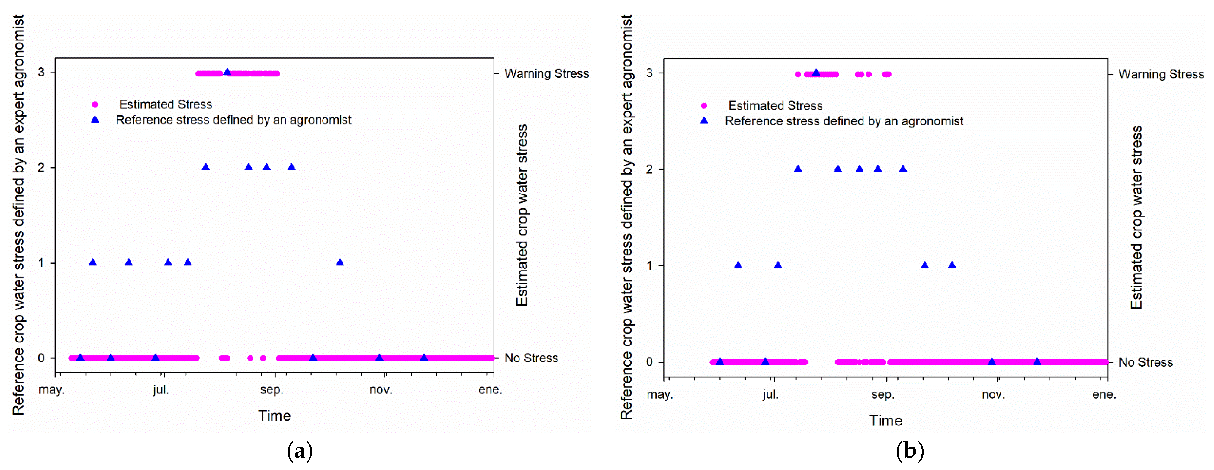
2.2. Crop Water Status Measurement

Crop water status was measured approximately every 10–15 days at 12:00–13:30 h (solar time) by determining midday Ψ_stem with a Scholander pressure chamber (Model 3000, Soil Moisture Equipment, Santa Barbara, CA, USA), according to the methodology proposed by McCutchan and Shackel [26] on six trees per treatment, as described in [22]. To measure Ψ_stem, healthy mature leaves close to the trunk were chosen from the north quadrant in order to avoid solar exposure. The leaves were covered with aluminum foil and wrapped into small black polyethylene bags at least 2 h prior to measurement.

2.3. Soil Water and Meteorological Variables Measurement

The soil of the study site was moderately stony and had a sandy loam texture, with a particle size distribution of 67.5% sand, 17.5% silt and 15% clay, high organic matter content (6.3%) in the surface layer (5–35 cm depth), and acceptable active limestone (2.7%), high assimilable phosphorus (108.67 mg kg⁻¹) and adequate exchangeable potassium (0.32 meq 100 g⁻¹) contents. The irrigation water came from a well and presented an average EC (Electrical Conductivity) of 0.8 dS m⁻¹ at 25 °C.

Soil volumetric water content, θ_V, was determined with Enviroscan (Sentek Pty. Ltd., Adelaide, Australia) capacitance-based profile sensors at 20 and 40 cm depths. One Enviroscan access tube was installed for each replicate, located 0.23 m from the irrigation emitter and 1.5 m from the tree trunk. Soil matric potential, Ψ_m, was also measured at 25 and 50 cm depths using Decagon MPS6 granular matrix sensors (Decagon Devices Inc., Pullman, WA, USA) per depth and replicate, likewise located 0.23 m from the irrigation emitter. Both, θ_v and Ψ_m, were recorded with a Campbell Scientific CR1000 datalogger (Campbell Scientific Inc., Logan, UT, USA), programmed to measure every 30 s and provide the mean value every 10 min.

Meteorological data on air RH (Relative Humidity), cumulative rainfall, solar radiation, air temperature and wind speed were provided hourly by a weather station close to the experimental site owned by the integral consulting service in agriculture SIAR (Sistema de Información Agroclimático para Regadío) [27]. In the case of solar radiation, wind speed, air RH and air temperature, we used hourly mean values, whereas the rainfall was the total accumulated every hour. From air temperature and RH data, we computed VPD according to [23].

2.4. Dataset Arrangement

The dataset used to train and test the crop water stress prediction models was built from the soil, plant and weather variables described above and recorded throughout 2015–2018 for the different irrigation treatments. The input variables were: soil water content at 20 (θ_v20) and 40 cm depth (θ_v40); soil matric potential at 25 (Ψ_m25) and 50 cm depth (Ψ_m50); air RH (air_RH); solar radiation (ϕ); air temperature (air_Temp); wind speed (WS); VPD; rainfall; DOY (Day Of the Year) and harvest period. The output variable was crop water stress, either expressed as a numerical pressure Ψ_stem value in MPa, or as categorical stress levels defined on the basis of the Ψ_stem value and the phenological stage, depending on the modeling approach used. For the classification approach, we defined a binary problem with two crop water stress classes: ‘no stress’ and ‘warning stress’. The categorization was based on the Ψ_stem value and the phenological stage according to the rule defined in

Table 1. Defined rule for binary categorization of crop water stress.

Harvest Period	Rule	Category
Pre-harvest	Ψstem > −0.9 MPa	‘no stress’
	Ψstem < −0.9 MPa	‘warning stress’
Post-harvest	Ψstem > −1.2 MPa	‘no stress’
	Ψstem < −1.2 MPa	‘warning stress’

.

The sampling frequency of soil and weather variables and Ψ_stem was uneven due to the limitations associated with the measurement of the latter, as described above. Thus, while soil variables were recorded every 10 min, weather variables were obtained every hour and Ψ_stem was measured, approximately, every 10–15 days. Taking into account that the dynamics of the soil–plant–atmosphere continuum involve dilated transient times and that a time series of soil and meteorological data is available before every measurement of Ψ_stem, we considered whether the time evolution of the physical input variables of the system, and more specifically the energy stored by these variables over a period of time, could be a relevant indicator for determination of the crop water stress. To compute the energy stored by the physical variables, the area under the curve described by these variables over a period of time, T, was calculated using a discrete integration method based on the calculation of trapezoidal areas, implemented in Matlab (version 2018a, MathWorks, Natick, MA, USA) with the trapz function. Thus, the disparity of the sampling frequency was also removed.

Intuitively, the time period considered in the integration of the input variables was a factor to take into account, since a priori the influence that these variables might have on Ψ_stem in the short and long term was unknown. We set days as the time unit. Considering D as the day for which an estimation of the tree water status was desired, we arbitrarily defined three time periods immediately prior to that day D: T = 3, 6 and 10 days. We defined the inputs of the models as the daily integrals of each soil and weather variable for each T (one variable per day), hereinafter called daily dynamics, and also added their cumulative values over the entire T period, hereinafter called accumulated dynamics. Therefore, three different datasets were defined. Therefore, for instance, for the dataset associated with T = 3 days, the model input variables defined from θ_v20 were θ_{v20_D1}, θ_{v20_D2}, θ_{v20_D3} and θ_{v20_ACCUM} (T = 3), which refer to the integral of θ_v20 over the day before D, the second-to-last day before D, the third-to-last day before D and the cumulative value of these, respectively.

Due to occasional sensor failure and breakdowns in the data acquisition system, several periods of soil data were lost unevenly among the different irrigation treatments, making the Ψ_stem data obtained throughout these periods unusable for the purpose of this study. In addition, no data were available for one of the replications of the FMR treatment. In summary, the number of Ψ_stem measurements used in this study and, consequently, the number of examples in the datasets for either value of T, was 389. A summary of the different models’ inputs considered in the study is presented in

Table 2. List of models’ inputs considered in the study.

Soil Variables	Weather Variables	Calendar Variables
θv20_Di, i = 1, …, T	air_RHDi, i = 1, …, T	DOY
θv20_ACCUM(T)	air_RHACCUM(T)
θv40_Di, i = 1, …, T	ϕDi, i = 1, …, T	Harvest period
θv40_ACCUM(T)	ϕACCUM(T)
Ψm25_Di, i = 1, …, T	air_TempDi, i = 1, …, T
Ψm25_ACCUM(T)	air_TempACCUM(T)
Ψm50_Di, i = 1, …, T	WSDi, i = 1, …, T
Ψm50_ACCUM(T)	WSACCUM(T)
	VPDDi, i = 1, …, T
	VPDACCUM(T)
	rainfallDi, i = 1, …, T
	rainfallACCUM(T)

T = 3, 6 or 10 days.

.

2.5. Modeling Approaches

In order to estimate tree water status from soil, weather and calendar data, analysis was carried out using two different approaches.

2.5.1. Binary Supervised Classification of Tree Water Status

From an agronomic point of view, it is of interest to determine whether a tree undergoes strong variations in its water status and reaches extreme stress conditions that can have transformative effects on the harvest in the current year or even the following year, especially when it is subjected to deficit irrigation. That is to say, the interest lies in creating an alarm system to determine whether the tree will reach a severe state of water stress than can endanger the eventual integrity of the crop, without giving importance to the magnitude of the stress. A priori, a binary classification approach can be considered to be less stringent than a precise estimation of the value of Ψ_stem per se. Therefore, we considered it appropriate to assess predictive binary classification models and defined the two classes as ‘no stress’ and ‘warning stress’ water stress states.

Within this approach, it should be noted that the available data give rise to an imbalanced binary classification problem, since only 26 out of the 389 total examples correspond to the ‘warning stress’ class, whereas the rest correspond to the ‘no stress’ class. In order to tackle this, the analysis was carried out in two different scenarios:

• By directly applying a ML classification technique, i.e., without taking into account the problem of imbalanced classes.
• By previously applying an oversampling technique to compensate for the sample size of both classes. Specifically, we applied MWMOTE (Majority Weighted Minority Oversampling Technique for imbalance dataset learning) [28], which is included in the R ‘imbalance’ package [29]. MWMOTE is a modification of the SMOTE technique [30], which overcomes some of its limitations when there are noisy instances, in which case SMOTE would generate additional noisy instances from them.

In turn, we applied two ML classification algorithms whose effectiveness is well-known [31,32,33,34]: RF (Random Forest) and SVM (Support Vector Machine). RF was implemented with R packages caret [35] and random Forest [36], whereas for SVM, we used R packages caret and kernlab [37]. We applied 10-fold CV (Cross Validation) throughout the whole dataset with 389 examples, obtaining the average of three repetitions, for the tuning of the hyperparameters mtry in RF and C (Cost) in SVM, applying Radial Basis Kernel in the latter. The hyperparameters were optimized to maximize the accuracy of the models, as set by default in the R packages used. In order to test the models, once the optimized hyperparameter was set, we applied LOO (Leave One Out) and computed the following performance metrics:

$$Accuracy=\frac{TP+TN}{TP+FP+TN+FN}$$

(1)

$$Recall \left(sensitivity\right)=\frac{TP}{TP+FN}$$

(2)

$$Specificity=\frac{TN}{TN+FP}$$

(3)

$$Precision=\frac{TP}{TP+FP}$$

(4)

$$F1 score=2\times \frac{Precision\times Recall}{Precision+Recall}$$

(5)

$$F2 score=5\times \frac{Precision\times Recall}{4\times Precision+Recall}$$

(6)

where TP, FP, TN and FN are True Positives, False Positives, True Negatives and False Negatives, respectively.

It should be noted that in this context of imbalanced classes, the accuracy metric is not sufficiently representative of the actual performance of the models, as its own value is biased towards the majority class. Therefore, when having imbalanced classes, with the minority class being the one of greatest agronomic interest in this case, it is essential to give special attention to metrics such as recall and F2 score. Recall is a metric that provides relevant information when there is a high cost associated with FN [38], as in the case of this study. Therefore, considering that the objective of the model is to detect ‘warning stress’ episodes, ‘warning stress’ would be the positive class and ‘no stress’ the negative class. Thus, FN would imply that a ‘warning stress’ episode would be classified as ‘no stress’. Precision is also a metric that focuses on the minority class, but should be preferred when FP are critical [38]. In the case of this study, having FP to a moderate extent should not be an issue, since the model would err on the side of security. F1 provides a balance between recall and precision, whereas F2 acts similarly, but putting more attention on minimizing FN [39], which is more relevant for the case of the study.

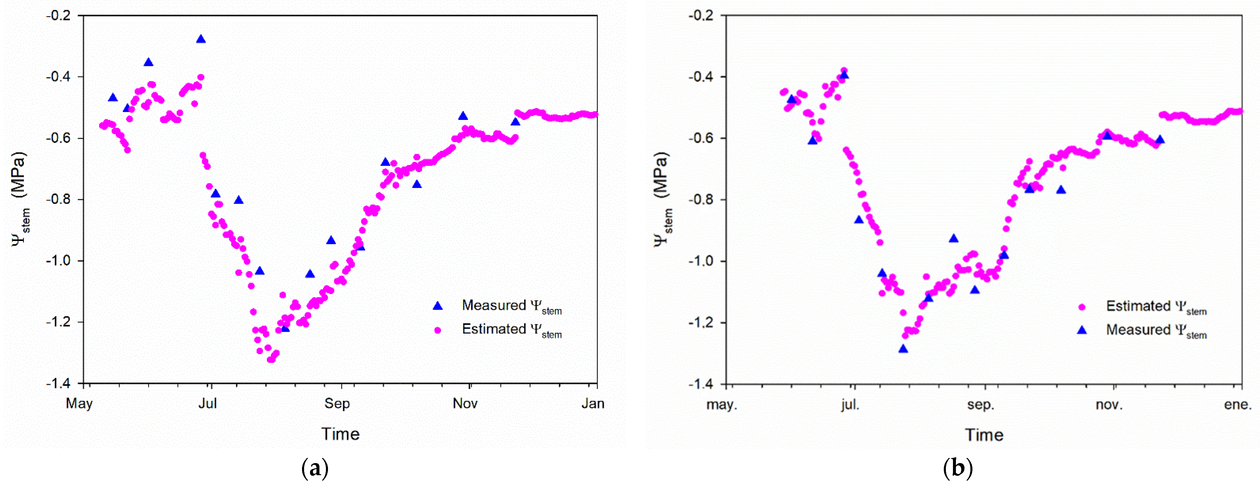
2.5.2. Ψ_stem Estimation with Regression Techniques

Alternatively, the water status of the tree can be assessed from its Ψ_stem, which is a continuous variable. The estimation of Ψ_stem using a regression problem, although more informative, may be more difficult to achieve. This approach, if successful, allows for estimation of the tree’s water condition, as well as the magnitude of water stress and its evolution over time. For this reason, it is opportune to assess predictive regression models.

In this case, we applied the same two ML techniques (RF and SVM), but for regression problems, optimizing the hyperparameters to minimize the RMSE. We evaluated the models using the following performance metrics:

$$ME\left(Mean Error\right)=\frac{1}{N}{\displaystyle \sum }_{\mathrm{i}=1}^N\left({\hat{\mathsf{\Psi }}}_{\mathrm{s}\mathrm{t}\mathrm{e}\mathrm{m},\mathrm{i}}-{\mathsf{\Psi }}_{\mathrm{s}\mathrm{t}\mathrm{e}\mathrm{m},\mathrm{i}}\right)$$

(7)

$$RMSE\left(Root Mean Square Error\right)=\sqrt{\frac{1}{N}{\displaystyle \sum }_{\mathrm{i}=1}^N{\left({\hat{\mathsf{\Psi }}}_{\mathrm{s}\mathrm{t}\mathrm{e}\mathrm{m},\mathrm{i}}-{\mathsf{\Psi }}_{\mathrm{s}\mathrm{t}\mathrm{e}\mathrm{m},\mathrm{i}}\right)}^2}$$

(8)

$$R^2=\frac{{{\displaystyle \sum }}_{\mathrm{i}=1}^N{\left({\hat{\mathsf{\Psi }}}_{\mathrm{s}\mathrm{t}\mathrm{e}\mathrm{m},\mathrm{i}}-{\overline{\mathsf{\Psi }}}_{\mathrm{s}\mathrm{t}\mathrm{e}\mathrm{m}}\right)}^2}{{{\displaystyle \sum }}_{\mathrm{i}=1}^N{\left({\mathsf{\Psi }}_{\mathrm{s}\mathrm{t}\mathrm{e}\mathrm{m},\mathrm{i}}-{\overline{\mathsf{\Psi }}}_{\mathrm{s}\mathrm{t}\mathrm{e}\mathrm{m}}\right)}^2}$$

(9)

$$MAPE\left(Mean Absolute Percentage Error\right)=\frac{100}{N}{\displaystyle \sum }_{\mathrm{i}=1}^N\left|\frac{{\hat{\mathsf{\Psi }}}_{\mathrm{s}\mathrm{t}\mathrm{e}\mathrm{m},\mathrm{i}}-{\mathsf{\Psi }}_{\mathrm{s}\mathrm{t}\mathrm{e}\mathrm{m},\mathrm{i}}}{{\mathsf{\Psi }}_{\mathrm{s}\mathrm{t}\mathrm{e}\mathrm{m},\mathrm{i}}}\right|$$

(10)

where ${\mathsf{\Psi }}_{\mathrm{s}\mathrm{t}\mathrm{e}\mathrm{m},\mathrm{i}}$ and ${\hat{\mathsf{\Psi }}}_{\mathrm{s}\mathrm{t}\mathrm{e}\mathrm{m},\mathrm{i}}$ are the measured and estimated Ψ_stem values of the ith example, respectively, ${\overline{\mathsf{\Psi }}}_{\mathrm{s}\mathrm{t}\mathrm{e}\mathrm{m}}$ is the mean value of Ψ_stem in the dataset and N is the number of examples in the dataset, i.e., N = 389.

Additionally, we explored the discriminatory ability of the models obtained with the regression approach to distinguish between ‘no stress’ and ‘warning stress’ classes by establishing specific thresholds. We evaluated this ability using ROC curves and the AUC (Area Under the Curve). From estimations of the stem water potential with the regression models, we defined several threshold values of stem water potential, such that below the threshold we considered the class to be ‘warning stress’ and above the threshold ‘no stress’. Thus, we performed a binary classification based on the estimated stem water potential (Ψ_stem) values obtained with the regression models. By sweeping the values of the threshold, we computed the classification metrics recall and specificity based on the estimated and actual crop water stress classes. The ROC curves were then obtained from the pairs of recall and specificity values.

2.6. Summary of Data Configurations Analyzed in the Study

In order to explore the influence that some of the input variables and the temporal format they are presented in can have on the estimation capabilities of the models, we defined several configurations. The study of these configurations allowed us to evaluate whether we could dispense with using either only soil moisture sensors or only soil matric potential sensors to account for relevant information regarding soil water; how determinant it would be to take into account both the daily and accumulated dynamics for the input variables; or if the VPD was representative of the other weather variables. The different configurations studied are presented in

Table 3. Model input configurations analyzed.

Configuration	Input Variables	N. of Inputs
1	All the inputs	22
2	All inputs but the daily dynamics	12
3	All inputs but θv dynamics	18
4	All inputs but the daily dynamics and θv dynamics	10
5	All inputs but Ψm dynamics	18
6	All inputs but the daily dynamics and Ψm dynamics	10
7	DOY, harvest period and Ψm and VPD dynamics	8
8	DOY, harvest period and Ψm and VPD accumulated dynamics	5
9	DOY, harvest period and θv and VPD dynamics	8
10	DOY, harvest period and θv and VPD accumulated dynamics	5

and the inputs referred to are those in Table 2.

3. Results and Discussion

3.1. Binary Supervised Classification Approach

In

Table 4. RF model classification performance metrics with the imbalanced dataset.

T	Metric	Input Configuration
		1	2	3	4	5	6	7	8	9	10
3 days	Accuracy	0.954	0.956	0.959	0.956	0.941	0.938	0.959	0.961	0.938	0.936
	Precision	0.750	0.800	0.727	0.696	0.600	0.625	0.727	0.720	0.571	0.538
	Recall	0.462	0.462	0.615	0.615	0.346	0.192	0.615	0.692	0.308	0.269
	Specificity	0.989	0.992	0.983	0.981	0.983	0.992	0.983	0.981	0.983	0.983
	F1	0.571	0.585	0.667	0.653	0.439	0.294	0.667	0.706	0.400	0.359
	F2	0.500	0.504	0.635	0.630	0.378	0.223	0.635	0.698	0.339	0.299
	TP	12	12	16	16	9	5	16	18	8	7
	FP	4	3	6	7	6	3	6	7	6	6
	TN	359	360	357	356	357	360	357	356	357	357
	FN	14	14	10	10	17	21	10	8	18	19
6 days	Accuracy	0.959	0.959	0.956	0.946	0.938	0.949	0.961	0.954	0.931	0.943
	Precision	0.778	0.857	0.737	0.647	0.625	0.650	0.789	0.722	0.400	0.643
	Recall	0.538	0.462	0.538	0.423	0.192	0.500	0.577	0.500	0.077	0.346
	Specificity	0.989	0.994	0.986	0.983	0.992	0.981	0.989	0.986	0.992	0.986
	F1	0.636	0.600	0.622	0.512	0.294	0.565	0.667	0.591	0.129	0.450
	F2	0.574	0.508	0.569	0.455	0.223	0.524	0.610	0.533	0.092	0.381
	TP	14	12	14	11	5	13	15	13	2	9
	FP	4	2	5	6	3	7	4	5	3	5
	TN	359	361	358	357	360	356	359	358	360	358
	FN	12	14	12	15	21	13	11	13	24	17
10 days	Accuracy	0.961	0.959	0.954	0.954	0.949	0.946	0.956	0.956	0.943	0.936
	Precision	0.789	0.778	0.700	0.682	0.750	0.647	0.737	0.696	0.700	0.529
	Recall	0.577	0.538	0.538	0.577	0.346	0.423	0.538	0.615	0.269	0.346
	Specificity	0.989	0.989	0.983	0.981	0.992	0.983	0.986	0.981	0.992	0.978
	F1	0.667	0.636	0.609	0.625	0.474	0.512	0.622	0.653	0.389	0.419
	F2	0.610	0.574	0.565	0.595	0.388	0.455	0.569	0.630	0.307	0.372
	TP	15	14	14	15	9	11	14	16	7	9
	FP	4	4	6	7	3	6	5	7	3	8
	TN	359	359	357	356	360	357	358	356	360	355
	FN	11	12	12	11	17	15	12	10	19	17

and

Table 5. RF model classification performance metrics with the MWMOTE-balanced dataset.

T	Metric	Input Configuration
		1	2	3	4	5	6	7	8	9	10
3 days	Accuracy	0.938	0.941	0.954	0.931	0.923	0.928	0.931	0.920	0.900	0.907
	Precision	0.531	0.552	0.625	0.486	0.433	0.467	0.486	0.444	0.303	0.368
	Recall	0.654	0.615	0.769	0.654	0.500	0.538	0.692	0.769	0.385	0.538
	Specificity	0.959	0.964	0.967	0.950	0.953	0.956	0.948	0.931	0.937	0.934
	F1	0.586	0.582	0.690	0.557	0.464	0.500	0.571	0.563	0.339	0.438
	F2	0.625	0.602	0.735	0.612	0.485	0.522	0.638	0.671	0.365	0.493
	TP	17	16	20	17	13	14	18	20	10	14
	FP	15	13	12	18	17	16	19	25	23	24
	TN	348	350	351	345	346	347	344	338	340	339
	FN	9	10	6	9	13	12	8	6	16	12
6 days	Accuracy	0.931	0.951	0.949	0.946	0.920	0.933	0.941	0.918	0.915	0.918
	Precision	0.480	0.621	0.615	0.581	0.407	0.500	0.552	0.417	0.394	0.406
	Recall	0.462	0.692	0.615	0.692	0.423	0.538	0.615	0.577	0.500	0.500
	Specificity	0.964	0.970	0.972	0.964	0.956	0.961	0.964	0.942	0.945	0.948
	F1	0.471	0.655	0.615	0.632	0.415	0.519	0.582	0.484	0.441	0.448
	F2	0.465	0.677	0.615	0.667	0.420	0.530	0.602	0.536	0.474	0.478
	TP	12	18	16	18	11	14	16	15	13	13
	FP	13	11	10	13	16	14	13	21	20	19
	TN	350	352	353	350	347	349	350	342	343	344
	FN	14	8	10	8	15	12	10	11	13	13
10 days	Accuracy	0.949	0.949	0.954	0.941	0.938	0.943	0.951	0.920	0.946	0.936
	Precision	0.600	0.600	0.667	0.552	0.536	0.571	0.630	0.442	0.581	0.515
	Recall	0.692	0.692	0.615	0.615	0.577	0.615	0.654	0.731	0.692	0.654
	Specificity	0.967	0.967	0.978	0.964	0.964	0.967	0.972	0.934	0.964	0.956
	F1	0.643	0.643	0.640	0.582	0.556	0.593	0.642	0.551	0.632	0.576
	F2	0.672	0.672	0.625	0.602	0.568	0.606	0.649	0.646	0.667	0.620
	TP	18	18	16	16	15	16	17	19	18	17
	FP	12	12	8	13	13	12	10	24	13	16
	TN	351	351	355	350	350	351	353	339	350	347
	FN	8	8	10	10	11	10	9	7	8	9

, we present a selection of the classification metrics of the RF model obtained with the imbalanced and MWMOTE-oversampling-balanced datasets, respectively. The different input configurations specified in Table 3, as well as the three time integration periods defined in Section 2.4, were evaluated. In order to provide a graphical overview of the metrics presented in Table 4 and Table 5 and to facilitate easier comparison among the different input configurations, input time integration periods and balanced and imbalanced datasets, in Figure 1 we graphically present the value of the most relevant metrics for the case of this study.

In all cases, except for Configuration 1 and T = 6 days, it is shown that the models trained with oversampled datasets resulted in a clear improvement in recall compared to the imbalanced-dataset-based models, at the cost of a very small loss of accuracy. This suggests that the oversampling method employed allowed the imbalanced binary classification problem to be solved. In Figure 1 it is also shown that, generally, the models trained with oversampled datasets improved over those trained with imbalanced ones on F1 and F2 metrics, especially the latter. Furthermore, the models trained with oversampled datasets showed less variability in F1 and F2, with T = 10 days being the most stable case for all input configurations.

For the RF model trained on the oversampled dataset for T = 10 days, we obtained an accuracy of 95% and recall of approximately 70% for several configurations. Even though the highest recall was obtained for T = 3 days in Configurations 3 and 8, T = 10 days performed better on average considering all configurations. In general, with the oversampled dataset, the difference in classification metrics between simpler models that include only accumulated dynamics and their corresponding complex versions, which also include daily dynamics, was not significant, especially for T = 10 days.

When weather variables were omitted, the use of the matric potential and DPV dynamics (configurations 7 and 8) yielded classification metrics that were among the highest, in many cases even higher than those of configurations that did include all weather variables.

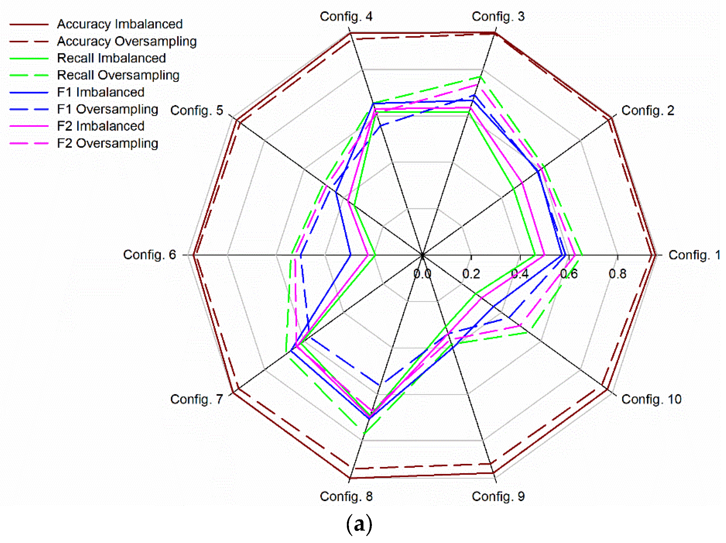
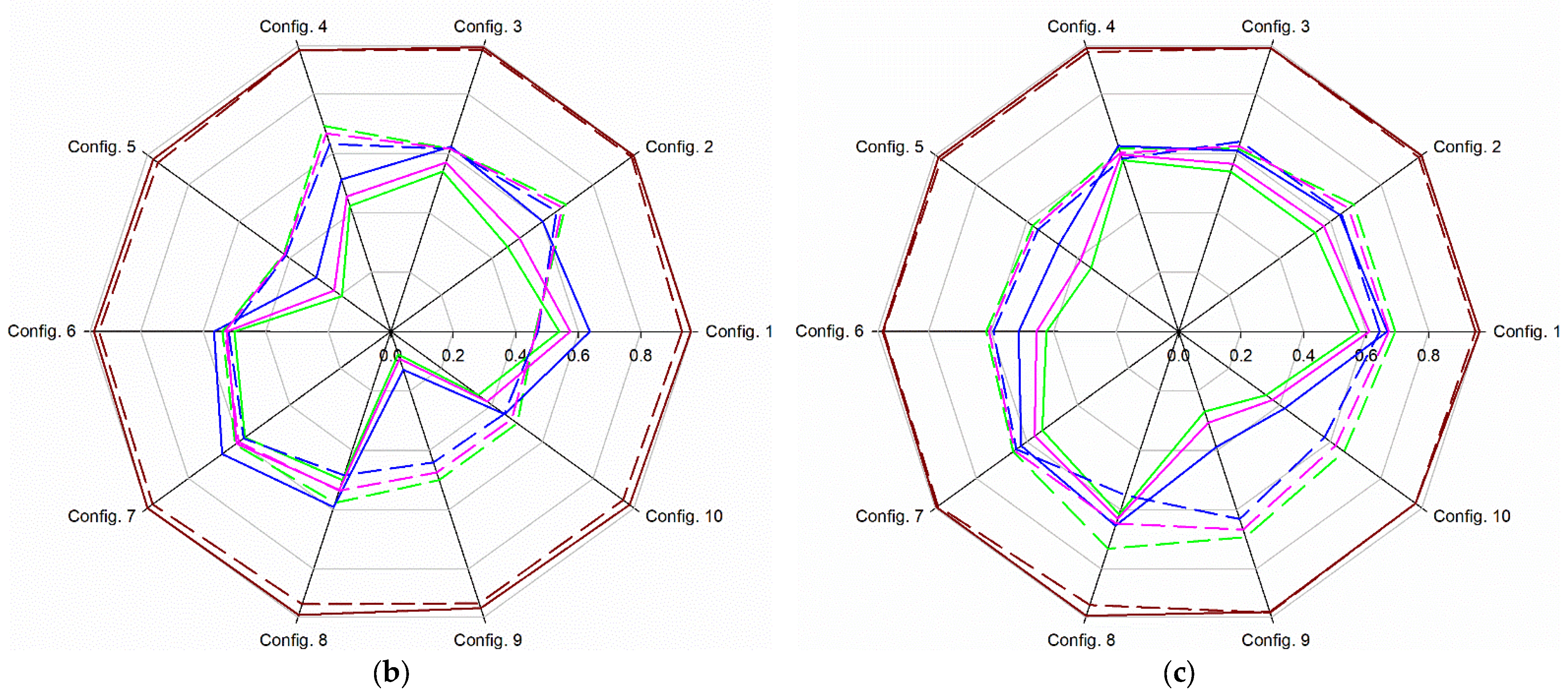
3.1.1. Influence of Soil Matric Potential and Soil Water Content on the Performance of the Models

Input Configurations 3 through 10 allowed us to evaluate the influence of using either soil moisture or soil matric potential sensors for tree water stress estimation. There is a wide variety of commercial and experimental soil moisture sensors and several measurement techniques, whereas only a few models of soil matric potential sensors can be found, the vast majority of them having limited pressure ranges. Generally, soil moisture sensors are available at a lower cost, yet soil matric potential offers a range of measurement of the water in soil that is available for the plant, which is a priori more relevant when studying soil–plant water interaction, as is the case here.

As shown in Table 4 and Table 5 and Figure 1, better classification metrics were found for configurations including Ψ_m instead of θ_v, even though the differences were dramatically reduced for T = 10 days. This suggests that the measured θ_v provides misleading information to the model in the short term in comparison with Ψ_m. Several factors, or even a combination of them, could be contributing to this, such as the proper heterogeneity of the soil, magnified by its stony nature; the way the Enviroscan sensor was installed in the soil, inside an access tube, which could produce considerable soil disturbance around the tube wall, altering the hydraulic conductivity of the soil; or a mismatch between the Enviroscan’s default calibration and the actual relationship between the dielectric properties of the soil and its water content, which is proven to be very dependent on soil texture, electromagnetic frequency and soil EC [40,41,42] and is not linear.

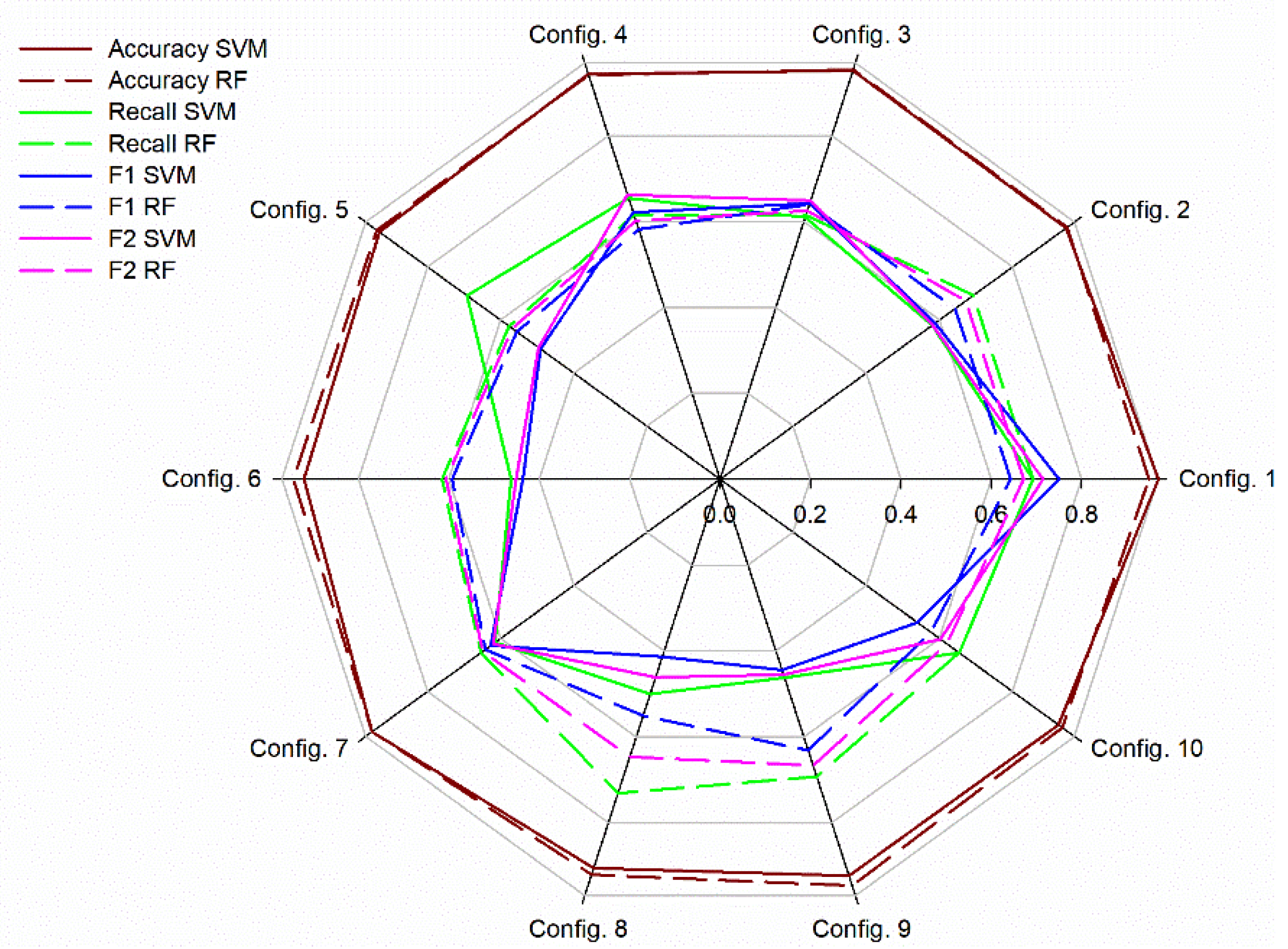
3.1.2. Comparison between RF and SVM Models

In

Table 6. SVM model performance metrics with the MWMOTE-balanced dataset.

T	Metric	Input Configuration
		1	2	3	4	5	6	7	8	9	10
10 days	Accuracy	0.969	0.946	0.951	0.943	0.931	0.920	0.951	0.905	0.923	0.925
	Precision	0.818	0.600	0.630	0.563	0.481	0.414	0.640	0.351	0.430	0.459
	Recall	0.692	0.580	0.61	0.654	0.692	0.462	0.615	0.500	0.462	0.654
	Specificity	0.989	0.972	0.972	0.961	0.961	0.953	0.975	0.934	0.956	0.945
	F1	0.750	0.588	0.642	0.621	0.491	0.436	0.627	0.413	0.444	0.540
	F2	0.714	0.581	0.649	0.662	0.496	0.451	0.620	0.461	0.455	0.603

, we present a representative example of the classification metrics for the SVM model with the MWMOTE-balanced dataset and T = 10 days, and in Figure 2 the most descriptive metrics are compared to those obtained with the RF model under the same conditions. The accuracy was similar with both models for every input configuration. Likewise, recall, F1 and F2 were similar for both models with most of the input configurations, with marked differences shown only for Configurations 6, 8 and 9, for which RF proved to be a better option. In this regard, it should be noted that SVM was applied with radial kernel, a technique which involves non-trivial tuning of several hyperparamaters with a high influence on the results obtained.

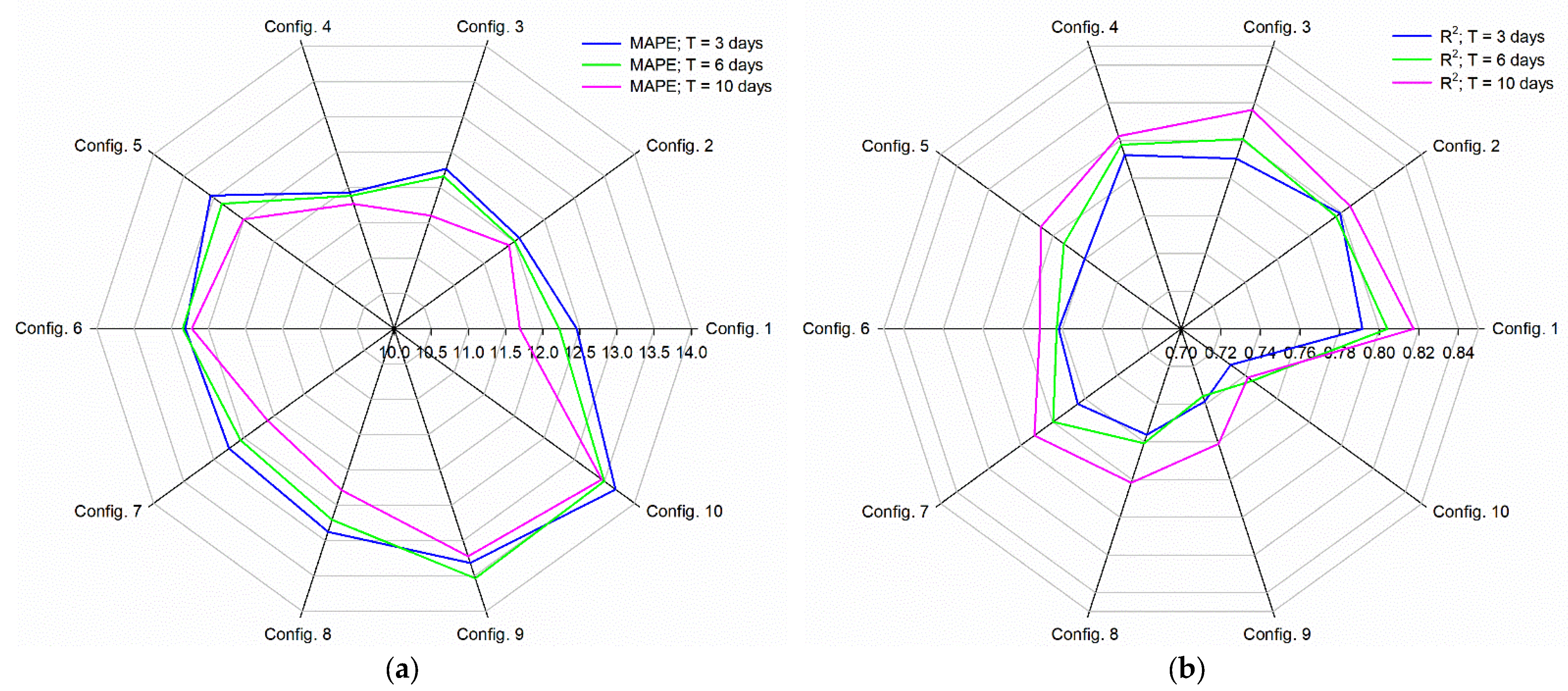
3.2. Regression Approach

For the regression approach, a higher performance was again observed with RF against SVM models. In

Table 7. RF model regression performance metrics.

T	Metric	Input Configuration
		1	2	3	4	5	6	7	8	9	10
3 days	ME	−0.004	−0.002	−0.004	−0.002	−0.002	−0.001	−0.005	−0.002	−0.002	−0.002
	RMSE	0.122	0.120	0.123	0.122	0.131	0.131	0.130	0.132	0.137	0.139
	R2	0.791	0.799	0.790	0.792	0.760	0.762	0.765	0.756	0.738	0.731
	MAPE	12.458	12.080	12.265	11.928	13.052	12.808	12.745	12.876	13.317	13.683
6 days	ME	−0.004	−0.002	−0.003	−0.001	−0.001	−0.002	−0.003	−0.002	−0.001	−0.002
	RMSE	0.118	0.121	0.119	0.120	0.127	0.130	0.126	0.131	0.138	0.135
	R2	0.804	0.797	0.801	0.798	0.773	0.763	0.780	0.761	0.736	0.745
	MAPE	12.223	12.005	12.159	11.883	12.865	12.843	12.554	12.705	13.533	13.493
10 days	ME	−0.003	−0.001	−0.003	−0.002	−0.002	0.000	−0.006	−0.002	−0.001	−0.001
	RMSE	0.114	0.118	0.115	0.119	0.123	0.128	0.122	0.125	0.131	0.136
	R2	0.817	0.805	0.816	0.802	0.788	0.771	0.792	0.782	0.761	0.742
	MAPE	11.691	11.914	11.600	11.768	12.507	12.722	12.105	12.287	13.222	13.454

, the regression performance metrics are summarized for RF with the different input configurations and T = 3, 6 and 10 days. In this regression approach, no oversampling was applied. The best goodness of fit was obtained for Configurations 1, 2, 3 and 4 for all T values, which again evidences the relevance of the information provided by the soil matric potential sensors together with the rest of the weather variables in the model, to the detriment of the less accurate information provided by the soil moisture sensors. The regression metrics obtained for T = 10 days were higher than those obtained with the rest of the integration periods, which suggests that the soil and meteorological states of up to at least 10 previous days have influence on the tree’s water status. As shown in Figure 3, generally, the use of both daily and accumulated dynamics provided slightly higher performance than using only the accumulated dynamics.

A coefficient of determination (R²) of up to 0.817 was obtained with Configuration 1 and T = 10 days. Intrigliolo and Castel [16] obtained an R² of 0.62 when correlating Ψ_m and Ψ_stem in plum trees, but no other soil or weather variables were considered in the model and the operating range of the Ψ_m sensors used was considerably more reduced than that of the ones used in the present study. Martí et al. [20] obtained higher R² of up to 0.926 in ‘Navelina’ citrus trees by using soil volumetric water content and weather data, but the dataset was limited to only 46 examples and only one RDI strategy was applied, thus demonstrating an outstanding performance in a specific reduced case, but more generalized models are expected when broadening the experimental conditions, as in the case of this study. Valdés-Vela et al. [21] evaluated the approach proposed by Martí et al. [20], in addition to a novel fuzzy rule based approach, on data from five different irrigation treatments with four replications each during five growing seasons, obtaining a RMSE of 0.141 in the best case, whereas with Configuration 1 and T = 10 days we managed to considerably reduce it to 0.114.

To evaluate the capability for discrimination between ‘no stress’ and ‘warning stress’ states by applying a threshold from estimations of Ψ_stem obtained with RF regression models, we obtained the ROC curves for T = 3, 6 and 10 days and the different input configurations. In Figure 4, the ROC curves for T = 10 days are presented as a representative example. Generally, from the ROC curves, the objective is to maximize the AUC. In

Table 8. AUC metrics for ROC curves obtained from binary classification applied using thresholds on the regression-estimated Ψ_stem.

T	Metric		Input Configuration
			1	2	3	4	5	6	7	8	9	10
3 days	AUC		0.974	0.971	0.970	0.966	0.952	0.951	0.964	0.958	0.938	0.937
	Deviation error 1		0.008	0.009	0.009	0.010	0.012	0.013	0.010	0.011	0.014	0.013
	Asymptotic signification 2		0.000	0.000	0.000	0.000	0.000	0.000	0.000	0.000	0.000	0.000
	95% asymptotic confidence interval	Lower bound	0.958	0.954	0.952	0.947	0.928	0.926	0.944	0.936	0.910	0.910
		Upper bound	0.990	0.988	0.988	0.985	0.976	0.976	0.985	0.980	0.965	0.963
6 days	AUC		0.972	0.965	0.970	0.960	0.955	0.952	0.964	0.954	0.936	0.945
	Deviation error 1		0.009	0.010	0.009	0.010	0.012	0.012	0.011	0.012	0.014	0.013
	Asymptotic signification 2		0.000	0.000	0.000	0.000	0.000	0.000	0.000	0.000	0.000	0.000
	95% asymptotic confidence interval	Lower bound	0.954	0.944	0.953	0.940	0.932	0.928	0.943	0.931	0.908	0.918
		Upper bound	0.990	0.985	0.988	0.981	0.978	0.976	0.985	0.978	0.964	0.971
10 days	AUC		0.974	0.968	0.972	0.960	0.962	0.956	0.966	0.951	0.963	0.944
	Deviation error 1		0.009	0.011	0.009	0.010	0.010	0.011	0.010	0.012	0.010	0.013
	Asymptotic signification 2		0.000	0.000	0.000	0.000	0.000	0.000	0.000	0.000	0.000	0.000
	95% asymptotic confidence interval	Lower bound	0.957	0.947	0.955	0.940	0.941	0.934	0.946	0.927	0.943	0.918
		Upper bound	0.992	0.989	0.989	0.981	0.983	0.978	0.985	0.975	0.984	0.970

¹ Under the non-parametric assumption. ² Null hypothesis: true area = 0.5.

, the AUCs for T = 3, 6 and 10 days and the different input configurations are presented. For all T values, Configurations 1, 2 and 3 were the ones providing the highest discriminatory ability, i.e., the greatest AUCs. However, these differences in discriminatory ability were not statistically significant, as indicated by the confidence intervals for the AUC presented in Table 8, i.e., for the same T value, since the intersection of all input configurations asymptotic confidence intervals is not an empty set, it could not be affirmed that there were differences between the AUCs of the different input configurations.

As an example application of this combined regression classification approach, from the ROC curve corresponding to T = 10 days and Configuration 2, two interesting thresholds could be found in terms of obtaining convenient recall and specificity. If the threshold was set at Ψ_stem = −1.102 MPa, so that an estimated Ψ_stem lower than that would be considered ‘warning stress’ and a higher one ‘no stress’, a recall of 88.5% and a specificity of 96.1% would be obtained. In this case, the specificity would indicate the likeliness of correctly predicting a ‘no stress’ case. Both recall and specificity were substantially high, but considering that avoiding ‘warning stress’ episodes is critical, a more conservative threshold, set at Ψ_stem = −0.845 MPa, would lead to a recall of 100% and a specificity of 82.9%. Therefore, this would avoid the risk of subjecting the tree to extreme stress by detecting all cases of potentially harmful stress, but at the same time it would generate an alert on a larger number of cases that were not really threatening, thus being on the side of safety. This would lead to the application of a slightly higher irrigation amount than needed by the crop in these cases in exchange for reducing the risk of unsafe water conditions for the tree.

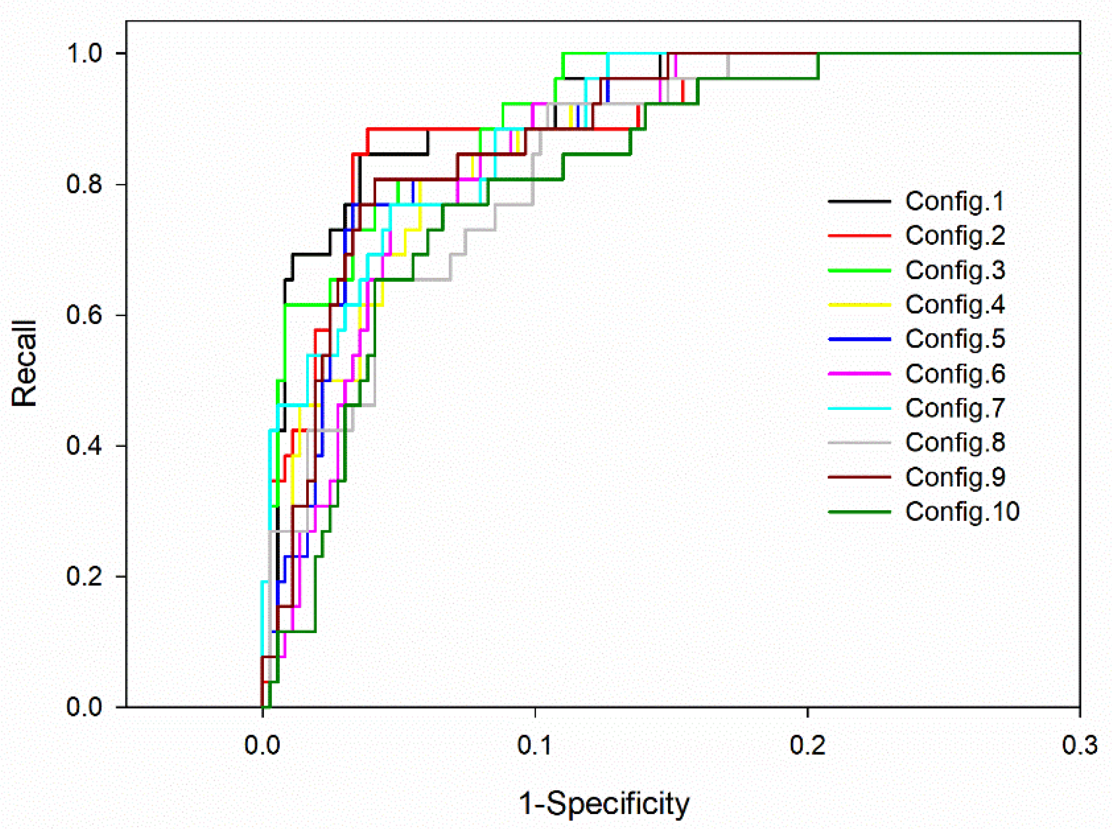
3.3. Classification Model Test

To assess classification model performance in predicting the water stress status of the crop during an arbitrary time period, we selected the RF model trained with the oversampled dataset and Configuration 2 for T = 10 days. The models were tested and their performance metrics obtained by means of the LOO method in Section 3.1. Here, we graphically evaluated the predictions of the model for days for which no Ψ_stem measurements were obtained, i.e., days from which the model was not trained. Thus, even though no objective metrics could be derived from this analysis, it did allow for observation of the consistency of predictions over time. In Figure 5, we present ‘no stress’ and ‘warning stress’ estimations (pink scatters) together with a reference four-level categorical stress defined by an agronomist (blue scatters) for irrigation treatments FMR (Figure 5a) and RDC-2 (Figure 5b) during 2015, as an example. These four categories of crop water stress were defined by an expert agronomist in a previous work [43] based on Ψ_stem measurements, harvest period and soil and weather time series data observations from the same dataset used in this study. These four stress categories corresponded to: 0, absence of stress; 1, light stress; 2, moderate stress; and 3, severe stress. In this study, we unified the stress categories 0, 1 and 2 into ‘no stress’, whereas stress category 3 corresponded to ‘warning stress’. Showing the reference stress divided into four categories in Figure 5 instead of the binary reference values provides information regarding how the crop water stress level evolves during the transition between ‘no stress’ and ‘warning stress’. The binary predictions were generally consistent with the reference data. The model kept the estimation at ‘no stress’ while the reference crop water stress level defined by the expert was 0 or 1. The model ‘alerted’ of ‘warning stress’ in the transition from expert-defined levels 1 to 2 and slightly fluctuated between ‘no stress’ and ‘warning stress’ during August, when the reference stress level was mainly 2 with a single case of level 3. However, in both cases presented, the model predicted ‘warning stress’ several days before level 3 was reached.

3.4. Regression Model Test

A similar approach to that in the previous section was adopted with the regression model. Likewise, we selected the RF model trained with Configuration 2 and T = 10 days as the best model and predicted Ψ_stem for those days that it had not been empirically measured. In Figure 6, the estimated and measured Ψ_stem are presented for the same irrigation treatments and times as in Figure 5. It can be noted that the predictions on the days when there were no Ψ_stem measurements follow the patterns and trends of the measured Ψ_stem fairly. At the lower and upper bounds of the Ψ_stem range presented in Figure 6a for the FMR irrigation treatment, i.e., when water was barely and highly available for the crop, respectively, the regression model tended to slightly underestimate the measured Ψ_stem values. Even though this behavior is not shown in the example presented for RDC-2 in Figure 6b, it was generally observed across the dataset. This means that the model would often predict slightly worse conditions than in the worst-case scenario for the crop water status, thus remaining on the side of security to manage crop health and productivity.

4. Conclusions

In this study we evaluated the performance of ML techniques to estimate the crop water stress of fruit trees, focusing the analysis on 15-year-old sweet cherry trees. We posed a novel model input format consisting of integrating the curve described by the input physical variables for a time period immediately before the day the estimation was going to be made. Two modeling approaches were tested: (i) a binary classification approach to determine whether the crop was subjected to tolerable (‘no stress’) or severe (‘warning stress’) water stress conditions and (ii) a regression approach to predict the numerical value of the tree stem water potential. As an alternative, this second approach was turned into a binary classification approach by defining a stem water potential threshold. The ML algorithms used were RF and SVM. We generally obtained higher performance with the former.

Modeling the crop water stress with the classification approach was challenging when using the original dataset due to its imbalanced condition, which provided limited examples of the minority class. The use of the MWMOTE oversampling method was critical to enhancing the performance of the model, increasing the recall and F1 and F2 scores and giving rise to more homogenous performance metrics among the different input configurations tested. The importance of the input configuration selected for the classification model was reduced as the inputs integration time increased, so that for T = 10 days, the performance of the model was leveled for all input configurations. This meant that the longer the input integration time, the lower the number of input variables needed to reach a similar classification performance. For the classification approach, the RF model trained with the oversampled dataset and Configuration 3 for T = 3 days and Configuration 2 for T = 10 days were the options which showed the highest performance in terms of accuracy, recall, and F1 and F2 scores. Generally, avoidance of soil water matric potential as an input to the classification model resulted in worse classification metrics, especially for reduced integration times (T = 3 and 6 days), and this was even more pronounced when the model was trained with the imbalanced dataset. Thus, soil matric potential sensors proved more accurate than soil moisture sensors in the estimation of crop water stress in the short term. Nevertheless, there is no evidence to confirm this in a generalized way. Further research is required with other sensors with different probe geometries and ways of installation, as well as with soil-specific calibration.

In the case of the regression approach, the input configurations including all soil and weather variables and those not including the soil moisture variables were the ones showing the best goodness of fit, revealing again the limited information provided by the soil moisture sensors used. It was also demonstrated that the longer the model input integration time, the better the model fit, at least up to 10 days, obtaining a R² of up to 0.817 with input Configuration 1; and that considering both daily and accumulated dynamics for the model inputs resulted in better estimations than using only accumulated dynamics. We also evidenced that from the crop stem water potential predicted with the regression model, an alarm system based on a Ψ_stem threshold could be set to inform the farmer of a potential crop water stress risk. Setting the threshold at Ψ_stem = −0.845 MPa for the RF regression model, with input Configuration 2 and T = 10 days, would detect every potential severe crop water stress episode.

Once the crop water stress estimation models developed in this study prove successful for preventive deficit irrigation management in sweet cherry trees, future work should be focused on extending this method and these models to other crops. Hypothetically, different crops and different soil conditions would change the parameters of the models. Additionally, the use of different soil moisture sensors would allow for clarification of the actual importance of this variable in the models.

References

1. Faurès, J.M.; Bartley, D.; Bazza, M.; Burke, J.; Hoogeveen, J.; Soto, D.; Steduto, P. Climate-Smart Agriculture Sourcebook; FAO: Rome, Italy, 2013; ISBN 978-92-5-107720-7. [Google Scholar]
2. IPCC. Climate Change and Water Technical Paper of the Intergovernmental Panel on Climate Change; IPCC: Geneva, Switzerland, 2008. [Google Scholar]
3. Santos Pereira, L.; Cordery, I.; Iacovides, I. Coping with Water Scarcity: Addressing the Challenges; Springer: Dordrecht, The Netherlands, 2009; ISBN 9781402095788. [Google Scholar]
4. Confederación Hidrográfica del Segura. Plan Hidrológico de la Demarcación del Segura 2015/2021; Ministerio de Agricultura, Alimentación y Medio Ambiente, 2015. Available online: https://www.chsegura.es/export/descargas/planificacionydma/planificacion15-21/docsdescarga/DIE_PHC_2015-21.pdf (accessed on 12 April 2022).
5. Ruiz-Sanchez, M.C.; Domingo, R.; Castel, J.R. Deficit irrigation in fruit trees and vines in Spain. Span. J. Agric. Res. 2010, 8, 5–20. [Google Scholar] [CrossRef] [Green Version]
6. Vera, J.; Abrisqueta, I.; Conejero, W.; Ruiz-Sánchez, M.C. Precise sustainable irrigation: A review of soil-plant-atmosphere monitoring. Acta Hortic. 2017, 1150, 195–202. [Google Scholar] [CrossRef]
7. Fereres, E.; Soriano, M.A. Deficit irrigation for reducing agricultural water use. J. Exp. Bot. 2007, 58, 147–159. [Google Scholar] [CrossRef] [PubMed] [Green Version]
8. Katerji, N.; Mastrorilli, M.; Rana, G. Water use efficiency of crops cultivated in the Mediterranean region: Review and analysis. Eur. J. Agron. 2008, 28, 493–507. [Google Scholar] [CrossRef]
9. Evans, R.G.; Sadler, E.J. Methods and technologies to improve efficiency of water use. Water Resour. Res. 2008, 44. [Google Scholar] [CrossRef]
10. Blaya-Ros, P.J.; Blanco, V.; Torres-Sánchez, R.; Domingo, R. Drought-Adaptive Mechanisms of Young Sweet Cherry Trees in Response to Withholding and Resuming Irrigation Cycles. Agronomy 2021, 11, 1812. [Google Scholar] [CrossRef]
11. Blanco, V.; Martínez-Hernández, G.B.; Artés-Hernández, F.; Blaya-Ros, P.J.; Torres-Sánchez, R.; Domingo, R. Water relations and quality changes throughout fruit development and shelf life of sweet cherry grown under regulated deficit irrigation. Agric. Water Manag. 2019, 217, 243–254. [Google Scholar] [CrossRef]
12. Blanco, V.; Torres-Sánchez, R.; Blaya-Ros, P.J.; Pérez-Pastor, A.; Domingo, R. Vegetative and reproductive response of ‘Prime Giant’ sweet cherry trees to regulated deficit irrigation. Sci. Hortic. 2019, 249, 478–489. [Google Scholar] [CrossRef]
13. Blanco, V.; Blaya-Ros, P.J.; Torres-Sánchez, R.; Domingo, R. Influence of Regulated Deficit Irrigation and Environmental Conditions on Reproductive Response of Sweet Cherry Trees. Plants 2020, 9, 94. [Google Scholar] [CrossRef] [Green Version]
14. Marsal, J. FAO irrigation and drainage paper 66. In Crop Yield Response Water. Sweet Cherry; FAO: Rome, Italy, 2012; pp. 449–457. [Google Scholar]
15. Shackel, K.A.; Ahmadi, H.; Biasi, W.; Buchner, R.; Goldhamer, D.; Gurusinghe, S.; Hasey, J.; Kester, D.; Krueger, B.; Lampinen, B.; et al. Plant water status as an index of irrigation need in deciduous fruit trees. Horttechnology 1997, 7, 23–29. [Google Scholar] [CrossRef] [Green Version]
16. Intrigliolo, D.S.; Castel, J.R. Continuous measurement of plant and soil water status for irrigation scheduling in plum. Irrig. Sci. 2004, 23, 93–102. [Google Scholar] [CrossRef]
17. Ortuño, M.F.; García-Orellana, Y.; Conejero, W.; Ruiz-Sánchez, M.C.; Mounzer, O.; Alarcón, J.J.; Torrecillas, A. Relationships between climatic variables and sap flow, stem water potential and maximum daily trunk shrinkage in lemon trees. Plant Soil 2006, 279, 229–242. [Google Scholar] [CrossRef]
18. Navarro-Hellín, H.; Martínez-del-Rincon, J.; Domingo-Miguel, R.; Soto-Valles, F.; Torres-Sánchez, R. A decision support system for managing irrigation in agriculture. Comput. Electron. Agric. 2016, 124, 121–131. [Google Scholar] [CrossRef] [Green Version]
19. Torres-Sanchez, R.; Navarro-Hellin, H.; Guillamon-Frutos, A.; San-Segundo, R.; Ruiz-Abellón, M.C.; Domingo-Miguel, R. A Decision Support System for Irrigation Management: Analysis and Implementation of Different Learning Techniques. Water 2020, 12, 548. [Google Scholar] [CrossRef] [Green Version]
20. Martí, P.; Gasque, M.; González-Altozano, P. An artificial neural network approach to the estimation of stem water potential from frequency domain reflectometry soil moisture measurements and meteorological data. Comput. Electron. Agric. 2013, 91, 75–86. [Google Scholar] [CrossRef]
21. Valdés-Vela, M.; Abrisqueta, I.; Conejero, W.; Vera, J.; Ruiz-Sánchez, M.C. Soft computing applied to stem water potential estimation: A fuzzy rule based approach. Comput. Electron. Agric. 2015, 115, 150–160. [Google Scholar] [CrossRef]
22. Blanco, V.; Domingo, R.; Pérez-Pastor, A.; Blaya-Ros, P.J.; Torres-Sánchez, R. Soil and plant water indicators for deficit irrigation management of field-grown sweet cherry trees. Agric. Water Manag. 2018, 208, 83–94. [Google Scholar] [CrossRef]
23. Allen, R.G.; Pereira, L.S.; Raes, D.; Smith, M. Crop evapotranspiration—Guidelines for computing crop water requirements. In FAO Irrigation and Drainage Paper 56; Food and Agriculture Organization: Rome, Italy, 1998; ISBN 92-5-104219-5. [Google Scholar]
24. Fereres, E.; Martinich, D.A.; Aldrich, T.M.; Castel, J.R.; Holzapfel, E.; Schulbach, H. Drip irrigation saves money in young almond orchards. Calif. Agric. 1982, 36, 12–13. [Google Scholar]
25. Blanco, V.; Blaya-Ros, P.J.; Castillo, C.; Soto-Vallés, F.; Torres-Sánchez, R.; Domingo, R. Potential of UAS-Based Remote Sensing for Estimating Tree Water Status and Yield in Sweet Cherry Trees. Remote Sens. 2020, 12, 2359. [Google Scholar] [CrossRef]
26. McCutchan, H.; Shackel, K.A. Stem-water Potential as a Sensitive Indicator of Water Stress in Prune Trees (Prunus domestica L. cv. French). J. Am. Soc. Hortic. Sci. 1992, 117, 607–611. [Google Scholar] [CrossRef] [Green Version]
27. SIAR. SIAR—Servicio Integral de Asesoramiento al Regante de Castilla-La Mancha. Available online: https://crea.uclm.es/siar/datosMeteorologicos (accessed on 23 February 2022).
28. Barua, S.; Islam, M.M.; Yao, X.; Murase, K. MWMOTE—Majority weighted minority oversampling technique for imbalanced data set learning. IEEE Trans. Knowl. Data Eng. 2014, 26, 405–425. [Google Scholar] [CrossRef]
29. Cordón, I.; García, S.; Fernández, A.; Herrera, F. Preprocessing Algorithms for Imbalanced Datasets Version 1.0.2.1; Institute for Statistics and Mathematics of WU (Wirtschaftsuniversität Wien): Vienna, Austria, 2020. [Google Scholar]
30. Chawla, N.V.; Bowyer, K.W.; Hall, L.O.; Kegelmeyer, W.P. SMOTE: Synthetic Minority Over-sampling Technique. J. Artif. Intell. Res. 2011, 16, 321–357. [Google Scholar] [CrossRef]
31. Giménez-Gallego, J.; González-Teruel, J.D.; Jiménez-Buendía, M.; Toledo-Moreo, A.B.; Soto-Valles, F.; Torres-Sánchez, R. Segmentation of Multiple Tree Leaves Pictures with Natural Backgrounds using Deep Learning for Image-Based Agriculture Applications. Appl. Sci. 2019, 10, 202. [Google Scholar] [CrossRef] [Green Version]
32. Oates, M.J.; González-Teruel, J.D.; Ruiz-Abellon, M.C.; Guillamon-Frutos, A.; Ramos, J.; Torres-Sánchez, R. Using a low-cost Components e-nose for Basic Detection of Different Foodstuffs. IEEE Sens. J. 2022, accepted (unpublished). [Google Scholar]
33. Cutler, A.; Cutler, D.R.; Stevens, J.R. Random Forests. In Ensemble Machine Learning; Zhang, C., Ma, Y., Eds.; Springer: Boston, MA, USA, 2012; pp. 157–175. ISBN 978-1-4419-9326-7. [Google Scholar]
34. Pisner, D.A.; Schnyer, D.M. Chapter 6—Support vector machine. In Machine Learning: Methods and Applications to Brain Disorders; Academic Press: Cambridge, MA, USA, 2020; pp. 101–121. ISBN 9780128157398. [Google Scholar]
35. Kuhn, M.; Wing, J.; Weston, S.; Williams, A.; Keefer, C.; Engelhardt, A.; Cooper, T.; Mayer, Z.; Kenkel, B.; R Core Team; et al. caret: Classification and Regression Training. R Package Version 6.0-86; Institute for Statistics and Mathematics of WU (Wirtschaftsuniversität Wien): Vienna, Austria, 2020. [Google Scholar]
36. Liaw, A.; Wiener, M. randomForest: Breiman and Cutler’s Random Forests for Classification and Regression. R Package Version 4.6-14. Available online: https://www.stat.berkeley.edu/~breiman/RandomForests/ (accessed on 1 February 2022).
37. Karatzoglou, A.; Smola, A.; Hornik, K.; National ICT Australia (NICTA); Maniscalco, M.A.; Teo, C.H. kernlab: Kernel-Based Machine Learning Lab version 0.9-29; Institute for Statistics and Mathematics of WU (Wirtschaftsuniversität Wien): Vienna, Austria, 2019.
38. Shung, K.P. Accuracy, Precision, Recall or F1? Available online: https://towardsdatascience.com/accuracy-precision-recall-or-f1-331fb37c5cb9 (accessed on 3 March 2022).
39. Brownlee, J. A Gentle Introduction to the Fbeta-Measure for Machine Learning. Available online: https://machinelearningmastery.com/fbeta-measure-for-machine-learning/ (accessed on 3 March 2022).
40. González-Teruel, J.D.; Jones, S.B.; Soto-Valles, F.; Torres-Sánchez, R.; Lebron, I.; Friedman, S.P.; Robinson, D.A. Dielectric Spectroscopy and Application of Mixing Models Describing Dielectric Dispersion in Clay Minerals and Clayey Soils. Sensors 2020, 20, 6678. [Google Scholar] [CrossRef] [PubMed]
41. González-Teruel, J.D.; Robinson, D.A.; Jones, S.B.; Skierucha, W.; Szyplowska, A. Impact of Effective Electromagnetic Frequency on Soil Moisture Sensor Calibration. In Proceedings of the ASA-CSSA-SSSA 2019 International Annual Meeting, San Antonio, TX, USA, 10–13 November 2019. [Google Scholar]
42. González-Teruel, J.D.; Torres-Sánchez, R.; Blaya-Ros, P.J.; Toledo-Moreo, A.B.; Jiménez-Buendía, M.; Soto-Valles, F. Design and Calibration of a Low-Cost SDI-12 Soil Moisture Sensor. Sensors 2019, 19, 491. [Google Scholar] [CrossRef] [Green Version]
43. González-Teruel, J.D.; Blanco, V.; Blaya-Ros, P.J.; Domingo, R.; Soto-Valles, F.; Torres-Sánchez, R. Estimación del Nivel de Estrés Hídrico en Frutales Mediante Técnicas Machine Learning para Aplicación en Sistemas de Riego Inteligentes. In Proceedings of the XLII Jornadas de Automática, Castellón de la Plana, Spain, 1–3 September 2021; Alonso Muñoz, A., Cabrera Santana, P.J., Chaos García, D., Déniz Suárez, Ó., Estévez Estévez, E., Guzmán Sánchez, J.L., Marín Prades, R., Muñoz de la Peña Sequedo, D., Peñarrocha Alós, I., Pitarch Pérez, J.L., et al., Eds.; Servizo de Publicacións da Universidade da Coruña: A Coruña, Spain; Comité Español de Automática: Barcelona, Spain; Universitat Jaume I: Castellón, Spain, 2021; pp. 477–484. [Google Scholar]
Figure 1. Comparison of RF model performance metrics for the different input configurations and the imbalanced and oversampling-based balanced datasets for T = 3 days (a), T = 6 days (b) and T = 10 days (c).
Agronomy 12 01422 g001aAgronomy 12 01422 g001b
Figure 2. Comparison of SVM and RF models’ performance metrics with different input configurations for the oversampling-based balanced datasets and T = 10 days.
Agronomy 12 01422 g002
Figure 3. MAPE (a) and R2 (b) regression metrics obtained with RF with the different input configurations for T = 3, 6 and 10 days.
Agronomy 12 01422 g003
Figure 4. ROC curves for threshold-based binary classification from regression-estimated Ψstem for all input configurations and T = 10 days.
Agronomy 12 01422 g004
Figure 5. Comparison of crop water stress level estimated with the classification RF model trained with Configuration 2 and T = 10 days and the reference crop water stress level defined by an expert agronomist in [43] for FMR (a) and RDC-2 (b) irrigation treatments during 2015.
Agronomy 12 01422 g005
Figure 6. Predictions of Ψstem obtained with the RF regression model trained with Configuration 2 and T = 10 days and measured Ψstem in FMR (a) and RDC-2 (b) irrigation treatments during 2015.
Agronomy 12 01422 g006