Article

Management Zones in Pastures Based on Soil Apparent Electrical Conductivity and Altitude: NDVI, Soil and Biomass Sampling Validation

1
MED—Mediterranean Institute for Agriculture, Environment and Development, Instituto de Investigação e Formação Avançada (IIFA), University of Évora, Pólo da Mitra, Ap. 94, 7006-554 Évora, Portugal
2
AgroInsider Lda., 7005-841 Évora, Portugal
3
Departamento de Expresión Gráfica, Escuela de Ingenierías Industriales, Universidad de Extremadura, Avenida de Elvas s/n, 06006 Badajoz, Spain
*
Author to whom correspondence should be addressed.
Agronomy 2022, 12(4), 778; https://doi.org/10.3390/agronomy12040778
Submission received: 14 February 2022 / Revised: 18 March 2022 / Accepted: 22 March 2022 / Published: 23 March 2022
(This article belongs to the Special Issue Selected Papers from 11th Iberian Agroengineering Congress)

Abstract

:
The intensification of the Montado mixed ecosystem (agro–silvo–pastoral) is a current endeavor in the context of promoting the sustainability of extensive livestock production in the Mediterranean region. Increased pasture productivity and extensive animal production involves the use of technologies to monitor spatial variability and to implement differentiated management of pasture grazing, fertilization or soil amendment. An intermediate step should lead to the identification and demarcation of areas with similar characteristics (soil and/or crop development), known as homogeneous management zones (HMZ) to implement site-specific management strategies. In this study, soil apparent electrical conductivity (ECa) and altimetry surveys were carried out in six experimental pasture fields with a non-contact electromagnetic induction sensor (EM38) associated with a Global Navigation Satellite System (GNSS) receiver. These ECa and topographic maps were used in geostatistical analyses for designing and establishing final classification maps with three HMZ (less, intermediate and more potential). The normalized difference vegetation index (NDVI), obtained from a proximal optical sensor, and soil and biomass sampling were used to validate these HMZ. From a practical perspective, these HMZ are the basis for preparation of fertilizer prescription maps and use of variable rate technology (VRT) in a Precision Agriculture project.

1. Introduction

Over the last decades, the world has witnessed increasing economic and environmental pressures on farmers. The increasing demand for food to feed a growing world population puts an enormous pressure on agricultural production [1]. At the same time, there is a trend for new environmental challenges, thereby increasing the need for environmental conservation practices [1]. The scientific community is responding to these challenges by developing sustainable ways to improve the efficiency of agricultural inputs, in order to maximize production and at the same time minimize environmental impacts [2].
Agro-forestry systems under semi-arid Mediterranean conditions, called Montado in Portugal and Dehesa in Spain, are mixed systems of trees (mainly Quercus suber and Quercus ilex species) with natural biodiverse pastures (grasses, legumes and other species) and scattered shrubs, and are grazed by animals, which has been proposed as a means for extending the benefits from forest to farmed land [3]. The understory vegetation of shrubs and pastures are the principal source of animal feed in extensive production systems [4]. Soil fertility is the main factor that determines pasture yield and quality [2,5]. Usually, due to intense erosion, the soils of these areas are degraded, shallow, acidic and stony and have low fertility (with low nutrient and organic matter content) while some soil properties exhibit a high spatial variability [2,5]. High spatial variability in soils is due to many physical, biological and chemical processes interacting simultaneously with different intensities [3,6]. Consequently, logical application of fertilizers or soil amendments should be based on an appropriate knowledge of the spatial variability of the main soil properties that can affect pasture yield and quality [7]. Therefore, assessing variability is the first critical step and a necessary condition for implementing strategies for management of this variability in the context of Precision Agriculture (PA) [8].
The most suitable and effective management strategy for intensifying and improving the economic feasibility of this silvo–pastoral ecosystem, with an associated increase in pasture productivity and, consequently, in extensive animal production, requires, as intermediate step involving the mapping of the spatial and temporal patterns of the main soil properties and determination of crop response [9], leading to the identification and demarcation of areas with similar characteristics (soil and/or crop development) [10]. These sub-regions of a field with similar soil fertility and production potential [10], with relatively homogeneous combination of yield-limiting factors, soil-landscape attributes [2] known as homogeneous management zones (HMZ) [6,9], can be used as a baseline for most farming decisions [2]. These decisions allow the implementation of site-specific management strategies [11,12], which culminate in the differential application of production factors, namely of fertilizers using variable rate technology (VRT) [9].
The delineation of HMZ requires collecting and analyzing data throughout the field, which involves the use of new technologies to monitor spatial variability [13]. Several approaches have been proposed to delineate HMZ at the field level. Data can be generated from a single data layer [2], the traditional soil sampling of the field and the subsequent laboratory work to obtain information on the main soil properties [14]. However, delineating zones based on soil physical properties most often captures yield variability due to differences in plant available water and, consequently, pasture production potential [14]. New research should make use of current sensor systems, which can gather data at sufficiently high density to characterize small-scale variations now known to be present in the majority of fields [2]. Therefore, HMZ are usually generated from a combination of data layers, including maps of crop yield, topography, soil chemical properties, aerial photographs, soil apparent electrical conductivity (ECa), or vegetation indices obtained by proximal or remote sensing [2,12].
Several studies have shown the practical interest and the potential of ECa monitoring for designing and establishing HMZ, implementing smart sampling, and elaborating prescription fertilizer maps [11]. This potential is due to the fact that this parameter integrates the main properties affecting crop productivity [2], namely, texture, soil moisture, organic matter content, and soil cationic exchange capacity [12,15]. Sensors to measure ECa in the field are of two types: contact, e.g., “Veris 2000 XA” model (Veris Technologies Inc., Salina, KS, USA) or non-contact, e.g., “EM38” (Geonics Ltd., Mississauga, ON, Canada), “GEM-2” (Geophex, Raleigh, NC, USA), or “DUALEM 1 S” (Dualem, Inc., Milton, ON, Canada). These sensors can be carried on mobile platforms mounted on a tractor or on an all-terrain vehicle, allowing quick ECa surveys and providing large amounts of information on various physical soil properties [8]. On the other hand, the use of vegetation indices obtained by proximal or remote sensing, to delineate HMZ in pastures, has deserved growing interest in the Mediterranean region, in particular, the works of Serrano et al. [3,9,16,17].
In regard to the HMZ validation process, there are many statistical methods to assess the relationship between vegetation indices (or other variables or attributes) and any other parameters [18]. These include a wide spectrum of methods, such as an exploratory analysis of the variables by means of descriptive statistics or a multivariate descriptive analysis to obtain the matrix of Pearson’s linear correlation coefficients, or other methods such as a canonical correlation analysis or an analysis of variance (ANOVA), to check whether classes arising from the clustering of indices or other variables provide effective management zones. When the assumptions of an ANOVA cannot be assured, the Kruskal–Wallis test and the Dunn test as a post-hoc analysis can be performed [19]. The use of a simple statistical index, such as the Kappa coefficient [20], to indicate the similarity between the maps generated with a reference map can be a suitable tool [21]. However, in the present study, a global index was defined to facilitate the validation process.
In this study, ECa and topographic surveys were carried out in six experimental fields with a non-contact electromagnetic induction sensor (“EM38”) associated with a GNSS receiver. The objective was to evaluate the soil spatial variability and generate HMZ maps of the soil fertility and, consequently, of the productive potential, the basis for smart sampling and the differential prescription of fertilizers. The normalized difference vegetation index (NDVI), obtained from a proximal optical sensor, and soil and biomass sampling were used to validate these HMZ through a global index.

2. Materials and Methods

Figure 1 shows a schematic representation of the methodology used in this study.

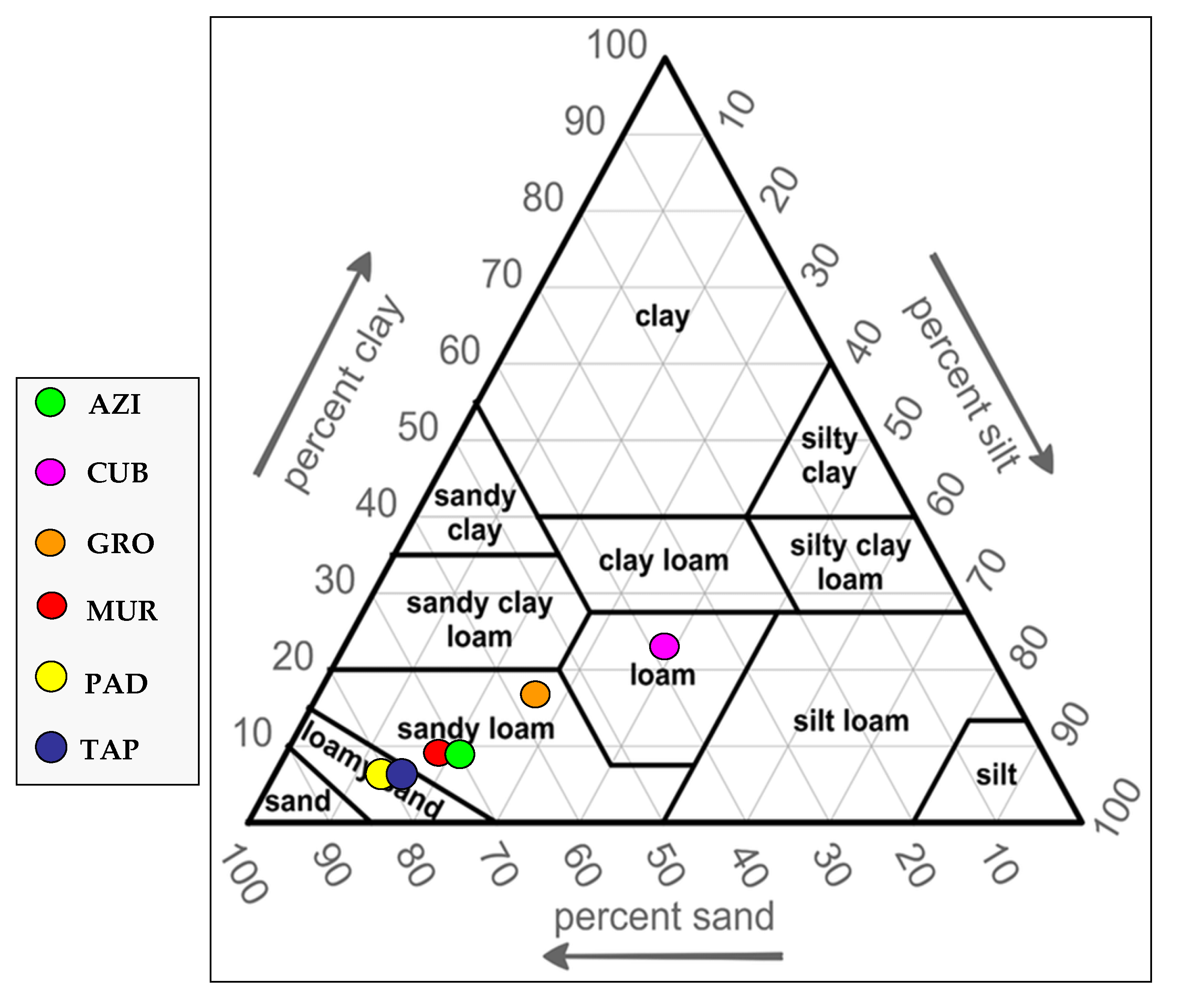
2.1. Characteristics of the Experimental Fields

This work was conducted in six experimental fields (“Azinhal”—“AZI”; “Cubillos”—“CUB”; “Grous”—“GRO”; “Murteiras”—“MUR”; “Padres”—“PAD”; and “Tapada”—“TAP”), five in the Alentejo southern region of Portugal (Beja, Évora and Portalegre districts) and one in Spain, near the Portalegre district (Figure 2). The main characteristics of the experimental fields used in this study are presented in Table 1. These are typical permanent seeded biodiverse dryland pastures that usually grow under a low or moderate density plantation of Holm oak or Cork oak, and are mainly used for grazing by cattle, sheep or pigs on a rotational basis. The soil type is Cambisol with a granite origin [22], characterized by slight or moderate weathering of parent material and by absence of appreciable quantities of illuviated clay, organic matter, aluminum, and/or iron compounds. These acid soils present medium to coarse texture (Table 1; Figure 3), are not very fertile and are mainly used for mixed agro–silvo–pastoral systems [23]. The location of these fields is representative of the temperate climatic conditions of Portugal (“Csa: hot-summer Mediterranean climate” according to the Köppen–Geiger climate classification), with a precipitation gradient: smaller amounts of rainfall in the southern district (“Beja”; mean annual rainfall of 430 mm), intermediate in the central district (“Évora”; mean annual rainfall of 567 mm) and greater in the northern district (“Portalegre”; mean annual rainfall of 950 mm) (source: Portuguese Institute of Sea and Atmosphere).

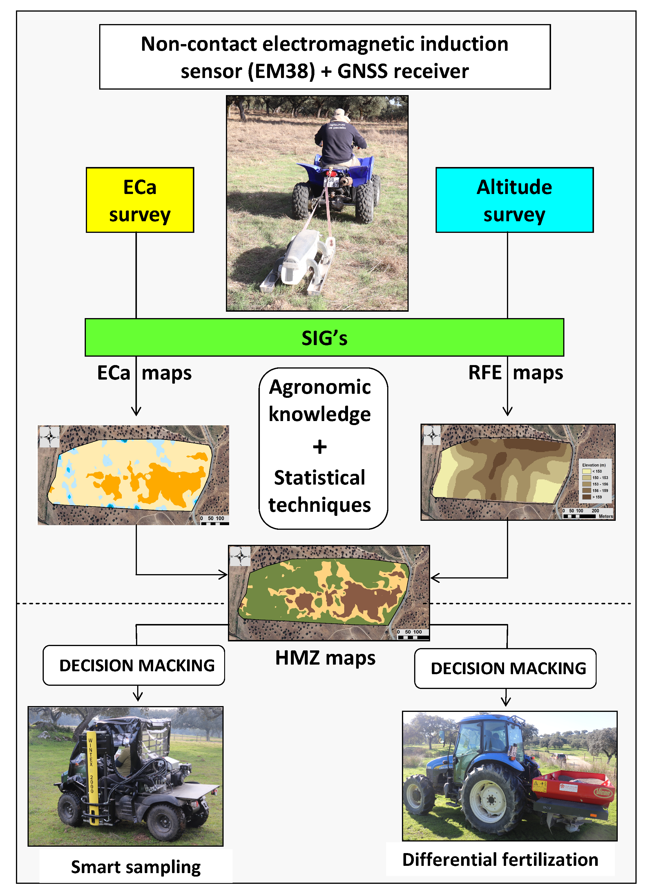
2.2. Soil Apparent Electrical Conductivity (ECa) and Topographic Survey

Soil apparent electrical conductivity (ECa) surveys were carried out at each experimental field in October 2019. A “EM38” device (Geonics Ltd., Mississauga, ON, Canada) was used in the horizontal dipole orientation with the two receiver coils separated by 0.5 m from the transmitter, providing data from effective depth ranges of 0.75 m and 0.375 m. In this study, only the data referring to the topsoil 0–0.375 m were used. The sensor was mounted on a metal-free sledge and pulled behind an all-terrain vehicle equipped with a GNSS receiver (see Figure 1), which simultaneously provided a topographic survey. The survey was carried out at an average speed of approximately 2.5 m s−1 and along parallel lines spaced 10 m, in order to cover the entire field. The ECa measurements were registered continuously every second, so the spatial resolution was a 2.5 by 10 m grid.

2.3. Soil Sampling and Laboratory Reference Analysis

For characterization of the topsoil (0–0.30 m depth), simultaneously with the ECa survey (October 2019), eight composite and georeferenced soil samples were collected in each experimental field using a gouge auger and a hammer. Each composite sample was the result of the combination of five sub-samples collected in an area of “10 m × 10 m” (Figure 4). These soil samples were inserted in plastic bags and transported to the “MED—Soil Analysis Laboratory” at University of Évora. The soil samples were weighed, dried at 70 °C for 48 h and then weighed again to establish the soil moisture content (SMC). Dried soil samples were analyzed for particle-size distribution (texture: sand, silt and clay content) using a sedimentographer (Sedigraph 5100, manufactured by Micromeritics, Norcross, GA, USA). The fine soil (fraction with diameter < 2 mm) was characterized in terms of pH, organic matter (OM), phosphorus (P2O5) and cationic exchange capacity (CEC). These fine components were analyzed using the following methods [24]: pH in 1:2.5 (soil: water) suspension, using the potentiometric method; OM by combustion and CO2 measurement, using an infrared detection cell; P2O5 was extracted by the Egner–Riehm method and measured using colorimetric method; CEC was measured by the neutral ammonium acetate method.

2.4. Normalized Difference Vegetation Index (NDVI) Measurements with Proximal Optical Sensor

Proximal optical sensor (AOS, OptRx, Ag Leader, Ames, Iowa, USA) measurements in each experimental field were carried out at the same eight georeferenced areas as the soil sampling (10 m × 10 m; Figure 4). This process was performed at four different times through the growth cycle, i.e., between January and June 2020 (Table 2). However, in “Cubillos” (“CUB”) experimental field (Located in Spain), due to road traffic restrictions imposed as a result of the COVID-19 pandemic, it was not possible to carry out two of the pasture collections (dates 3 and 4). The optical sensor (equipped with a small portable battery as the power source) was placed 0.5 m above the pasture and provided simultaneous measurement of three visible and infrared bands. With two of these spectral bands, red (670 nm) and near infrared (NIR, 775 nm), NDVI was calculated [16]. The AOS operator walked each sampling area for a five-minute period, which allowed the collection of approximately 300 NDVI records.

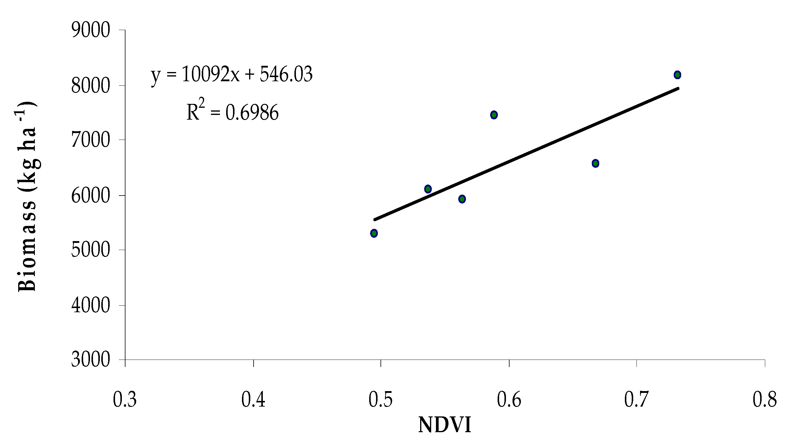
2.5. Pasture Biomass Sampling and Normalized Difference Vegetation Index (NDVI) Measurements

Pasture sampling in each experimental field was carried out at the same eight georeferenced areas as the soil sampling and proximal optical sensor measurements (10 m × 10 m; Figure 4). In each of these areas, composite pasture samples were obtained by collecting five subsamples with electric shears at 1 to 2 cm above ground in a 0.5 m × 0.5 m area (defined with a metal quadrat). The sampling process was performed at four different times through the growth cycle, i.e., between January and June 2020 (Table 2), except in “Cubillos” (“CUB”), due to the above mentioned restrictions. Pasture samples were inserted into numbered plastic bags and transported to the MED—Animal Nutrition and Metabolism Laboratory at the University of Évora. Once in the laboratory, the pasture samples were weighed to obtain the biomass (in kg ha−1).

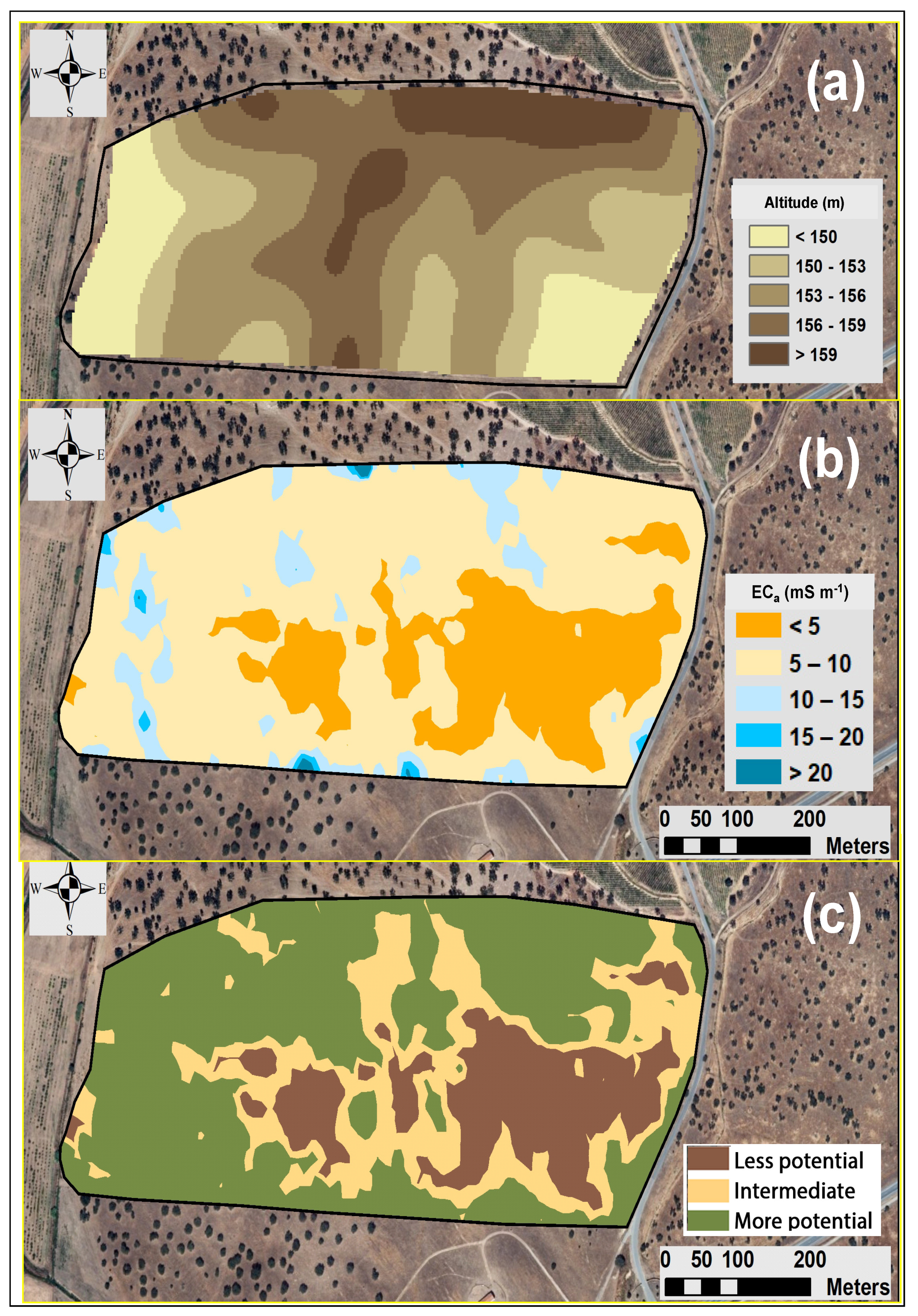
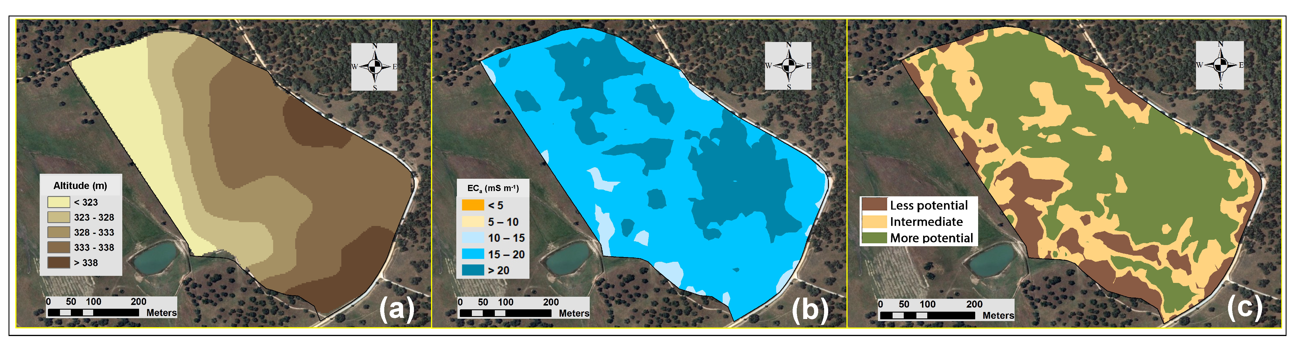
2.6. Soil Apparent Electrical Conductivity (ECa) and Topographic Altitude Processing

Estimating ECa at unsampled locations was carried out with the ordinary point kriging method. This produced kriged maps showing the spatial distribution of ECa in each experimental field based on the estimated values. Although there are many algorithms that can be used for interpolation, the advantages of using geostatistical techniques [25] are well recognized considering the spatial variation of the studied variable, which is ECa in this case. The geostatistical analyses were carried out with the extension, Geostatistical Analyst of ArcGIS (version 10.5, ESRI, Inc., Redlands, CA, USA), and the kriged maps of ECa were produced with the ArcMap module of ArcGIS software.
Digital elevation model (DEM) surfaces were generated for each field using the triangulated irregular network (TIN) interpolation tool from the ArcGIS. The TIN algorithm uses sample points to create a surface formed by triangles based on nearest neighbor point information. Then, the vector layers were converted into grid surfaces with the spatial analyst tools of ArcGIS.

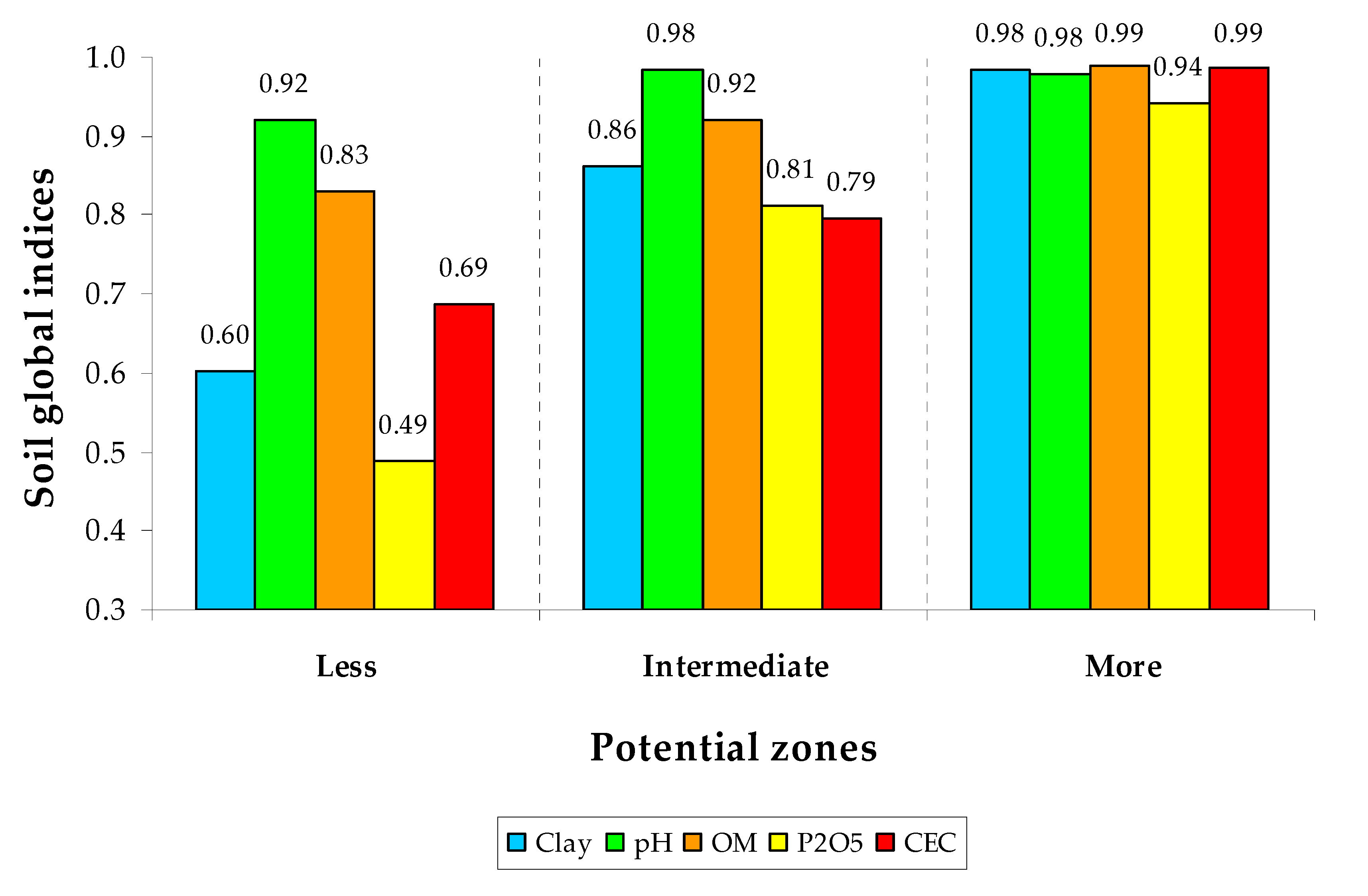
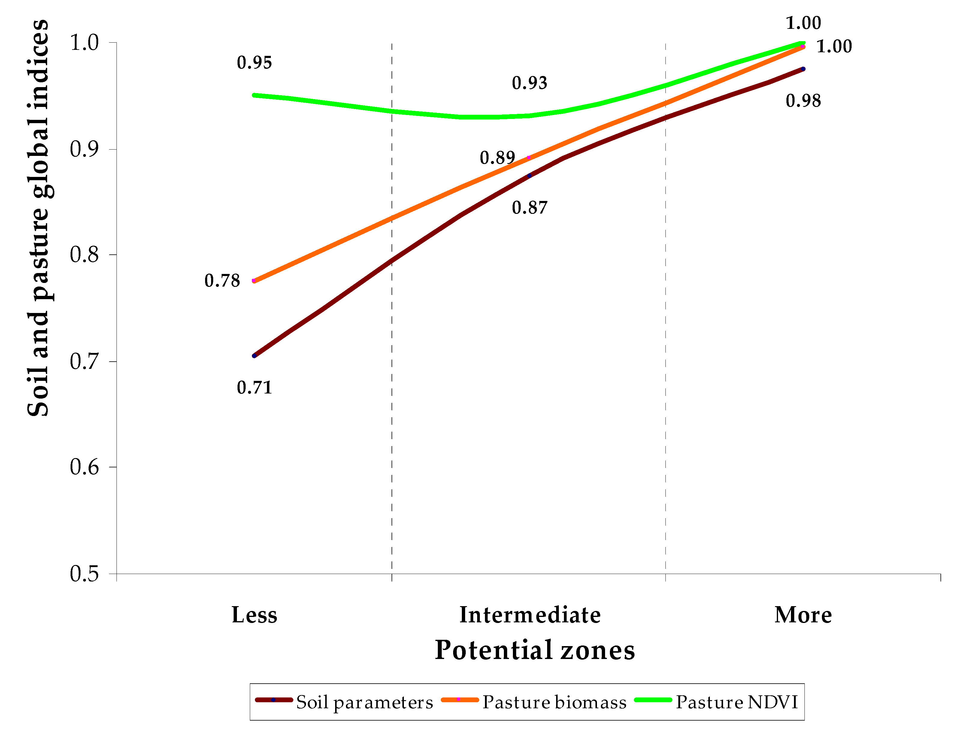
2.7. Definition and Validation of Homogeneous Management Zones (HMZ)

Descriptive statistical analysis (mean, standard variation and range) was performed for all soil and pasture parameters.
After obtaining the ECa maps for each field, homogeneous zones were delimited using a classification technique in ArcGIS. Topography was also considered since it is an important factor that can affect the potential zones [26]. Consequently, the final classified maps were generated using an unsupervised classification technique on two sets of input data: the ECa and the altitude layers. The ISO Cluster approach in ArcGIS was used to perform the classification. This algorithm organizes the data in the input raster into a user-defined number of groups to produce signatures, which are utilized to classify the data using the “Maximum Likelihood Classifier” (MLC) function. The number of groups was fixed at three in this study (less, intermediate and more potential), as only a few homogeneous zones should be delineated, from a practical perspective.
Soil parameters (texture, pH, OM, P2O5 and CEC), and pasture biomass and vegetation index (NDVI) data at sampling locations were employed to check their differences. The delimitation of each zone in each experimental field was evaluated by computing the differences in the mean values of these soil and pasture parameters. In the case of soil parameters, because they were based on a small number of samples (only 8 composite samples in each experimental field), they were used as an indication of trends. The pasture parameters (biomass and NDVI), resulting from 8 composite samples obtained on 4 dates (a total of 32 samples in each experimental field) were treated using the Kruskal–Wallis nonparametric test and the Dunn test as a post-hoc analysis in the IBM SPSS statistical package (version 24, IBM Corp, Armonk, NY, USA). These tests were chosen since the normality in the data cannot be assumed. The Kruskal–Wallis test is a rank-based non-parametric test that can be used to determine if there are statistically significant differences between two or more groups of an independent variable on a continuous or ordinal dependent variable. The Kruskal–Wallis test indicates that at least two groups were different but cannot indicate which specific groups of the independent variable are statistically significantly different from each other. Consequently, since more than two groups can be defined, determining which of these groups differ from each other was performed by means of the Dunn test as a post-hoc non-parametric test.
To facilitate the validation process of management zones based on soil and pasture samples, a global index (GI) was calculated for each parameter, in the set of six experimental fields. In this calculation, the coefficient “1” was assigned to the highest value of the parameter in each experimental field, in the set of 3 management zones. The value of the same parameter in the remaining two zones was transformed into a decimal fraction of this maximum value (relative value of each parameter, RV), corresponding to the ratio between the value in question and the maximum value (Equation (1)). After calculating the ratios, for each zone and each experimental field, the average value of the GI for each parameter in the set of six experimental fields was calculated (Equation (2)).
R V i j k = A V i j k M a x . V i , j = 1 . t o . m , k
G I j k = i = 1 n ( R V j k n )
where: RV—relative value of each parameter; AV—absolute value; Max.V—maximum value; i—location; j—homogeneous management zones; m—number of homogeneous management zones; k—parameter measured; n—number of locations of each j-k pair.

3. Results

Descriptive statistics of altitude, soil and pasture parameters for the six experimental fields are shown in Table 3, Table 4 and Table 5, respectively.
It is evident (Table 4) that soil clay content is generally low (<10%), while in two of the experimental fields, clay content is higher (17% in “Grous” and 23.5% in “Cubillos”). The pH of these soils is usually low (<6.0), except in “Padres” (mean of 6.4) and “Azinhal” (mean of 6.7), which explains the usual practice of applying lime amendment. Soil organic matter (OM) presents average values of 2.5–3%, except in “Azinhal” (1.9%) and “Tapada” (2.2%). Average P2O5 contents are low in all experimental fields (<30 mg kg−1), which explains the usual practice of applying phosphorous fertilizer in these dryland pastures. Average pasture productivity (biomass) varies between 5300 kg ha−1 (“Azinhal”) and 8164 kg ha−1 (“Cubillos”) (Table 5). It is important to highlight the high intra and inter field spatial variability (Table 4). The coefficient of variation (CV), for example, varies between 7% and 91% for clay, between 3% and 8% for pH, between 7% and 36% for OM, between 8% and 35% for CEC, between 16% and 77% for ECa, between 5% and 23% for SMC, between 30% and 80% for biomass and between 7% and 37% for NDVI. The seasonality of pasture production throughout the vegetative cycle is represented by the wide amplitude of the productivity (biomass) and of the vegetative vigor of the pasture (NDVI) in the set of six experimental fields: respectively between 1167 (“Azinhal”) and 18,603 kg ha−1 (“Murteiras”) and between 0.241 (“Grous”) and 0.819 (“Padres”). Figure 5 shows the significant linear correlation between the mean values of biomass and the mean values of NDVI, in the set of six experimental fields.
Figure 6, Figure 7, Figure 8, Figure 9, Figure 10 and Figure 11 show the altitude (a), ECa (b) and homogeneous management zone (c) maps of the six experimental fields.
Table 6 shows mean values of soil parameters (clay, pH, OM, P2O5 and CEC) in the management zones of each experimental field. Due to the small number of composite samples (only eight), they were used only as an indication of trends. Given that the establishment of sampling areas was carried out before the ECa and altitude surveys, and therefore, before the definition of the HMZ in some experimental fields (“Azinhal”, “Murteiras”, “Padres” and “Tapada”), one of the three identified zones was not sampled (soil and pasture). The trend for some soil properties, which are related to soil fertility, is in accordance with the proposed zoning. This is the case for CEC in “Azinhal”, “Cubillos”, “Grous”, “Murteiras” and “Tapada”, of clay contents in “Azinhal”, “Grous”, “Murteiras” and “Tapada” or OM in “Cubillos”, “Grous” and “Murteiras”, where higher values were found in zones with more soil fertility potential. When compared to other important soil parameters in Mediterranean pastures, the low levels of the P2O5 in all experimental fields, which is one of the main limitations of these soils, do not show a consistent trend, despite the areas with more potential in “Crous” and “Murteiras” registering clearly higher values of this nutrient. Among the five parameters considered in this study, soil pH seems to be the one with the lowest sensitivity for validating the management zones.
Figure 12 shows the GI calculated for five soil parameters based on Equations (1) and (2). This figure confirms that pH is the only soil parameter that does not allow the differentiation of the established HMZ. The remaining soil parameters (clay, OM, P2O5 and CEC) systematically show higher values in areas with more potential.
Table 7 shows mean values of pasture parameters (biomass and NDVI) in each management zone for each experimental field. Within each column, different letters indicate significant differences (p < 0.05) between zones performed by the Dunn test. Biomass was the most useful variable to characterize homogeneous zones, systematically presenting, in all experimental fields, significantly higher productivity values in zones with more potential. On the other hand, it was apparent that the use of NDVI was not suitable to differentiate HMZ, since mean values were similar in the various potential homogeneous zones in many experimental fields (“Cubillos”, “Murteiras” and “Padres”).
Figure 13 shows soil and pasture global indices: a soil fertility GI (including the set of all the measure soil parameters), a pasture biomass GI and a pasture NDVI GI. Both soil fertility GI and pasture biomass GI consistently differentiate the previously defined HMZ’s. However, pasture NDVI GI, similar to individual analysis, field by field (Table 7), did not show sufficient sensitivity to differentiate HMZ.

4. Discussion

Based on ECa and topographic surveys, the objectives of this study were: (i) to evaluate the soil spatial variability and generate HMZ maps; and (ii) validate these HMZ through soil, biomass and NDVI measurements.
In the last decade, numerous works have been published that replicate the use of ECa sensors and geostatistical techniques to define HMZ in very different crops, for example, in corn [27], vineyards [28], olive orchards [29] or pastures [9,10,15,30].
The methods used to validate HMZ are very diverse, with the intensive soil sampling being the most common process [5,31,32,33], but often it is not technically feasible for large-scale application [34]. In addition, some soil variables (such as the pH in our study) correlate inconsistently with ECa mainly as a consequence of complex interactions between soil properties [29], and a temporal component of variability that is only weakly detected by an expected constant variable such as ECa [35]. Alternatively, these soil properties can be used to formulate a soil fertility index [2,7]. The use of a global soil fertility index (GIsoil), such as the one presented in this study, that encompasses several relevant parameters with direct influence on soil fertility (including phosphorous, OM, pH, clay content and CEC), is a simplified approach which has been proposed in several works [2,7]. In this way, it is possible to reduce the complexity assumed by geostatistical techniques, based, for example, on the Rasch model clustering process [5,7] or on principal component analyses [2]. The GIsoil showed the ability to validate areas of different potential, identified through ECa and altitude data, which is in agreement with several other works [32,36,37].
The validation based on biomass assumes the well-studied relationship between soil characteristics and crop productivity [5,29]. In cereal crops (wheat, corn, among others), the incorporation of calibrated commercial yield monitors in combines equipped with differential GPS antenna provides crop yield maps [32], which is interesting spatial information for use as a validation tool specifically for this type of crop [2]. However, in livestock production systems, which is the case here, it is difficult to quantify the spatial variability of biomass production because forage is usually harvested by animals [6], which requires manual and representative sample collection. Alongside the GIsoil, the pasture yield (biomass) showed the ability to validate potential management zones defined in this study. However, since this is an exhaustive and expensive process, there is a growing interest in studies based on rapid sampling and validation methodologies [16]. One option increasingly used for this purpose [12] is indirectly via plant growth measurements that rely on vegetation indices [36]. Remote or proximal sensing provides an attractive opportunity to obtain the NDVI or other indices [12] related to pasture development throughout the vegetative cycle [16]. In this study, NDVI was not consistent in the validation of HMZ, which is in line with other studies [5]. One problem attributed to NDVI is its insensitivity to changes in environment and/or biomass when environmental conditions and biomass reach a certain threshold [16,38]. According to Moral et al. [14], the spatial variability detected by optical sensors at vegetation level is not related to the spatial pattern of soil fertility and not suitable to detect the spatial variability between zones. Serrano et al. [13] showed that NDVI reflects the plant chlorophyll content and, therefore, has greater potential to monitor the evolution of pasture quality, namely the crude protein content, than the productivity predicted in the three HMZ defined in this study.
The results of this study show the interest in multi-variable HMZ validation approaches, which consider soil and landscape attributes, yield data (biomass) and/or multi-temporal vegetation measurements (time-series of vegetation indices obtained by proximal or remote sensing) [12]. The combination of different validation methods can alleviate the difficulty in interpretating ECa readings, which are highly location and soil-specific [35].
Variability is a fundamental component of the PA concept. This associates an exponential incorporation of technology to support decision making in complex agricultural and livestock production scenarios [6]. The definition of HMZ meets the major aim of PA [2]: to optimize crop management by addressing spatial variability and thus optimizing the use of farm inputs [12]. For example, the published works of Cicore et al. [30], Moral et al. [5] or Bonecke et al. [33] show algorithms and methodologies to predict and quantify the needs for the variable rate application of nitrogen fertilizer, phosphorous fertilizer or lime amendment.
Soil spatial variability is one of the main parameters, especially in Montado’s Alentejo region, southern Portugal [4], impacting the productivity of dryland pastures and, consequently, the extensive animal production systems [39]. The results obtained in this study confirm this variability, reflected in the high soil coefficients of variation, intra and inter experimental fields, and highlight some of the main limitations of these soils: in general, low pH (mean between 5.5 and 6.7), usually with coarse texture and low amounts of phosphorous (P2O5 < 30 mg kg−1). The combination of these factors substantiates the widespread practice in these dryland pastures of soil phosphorous fertilization [4]. However, this is a complex process. Given that the relative agronomic effectiveness of phosphorus fertilizers and the availability of this nutrient in the soil environment is governed by reactions in the soil matrix that are highly influenced by the pH [40], pH correction might be required before P fertilizing [13]. Additionally, Carvalho et al. [41] mention the need to improve the Mg/Mn ratio in order to reduce the problems of Mn toxicity, which has long been recognized as the major limiting factor of pasture and forage production on acid cambisoils of Portugal. Therefore, these authors suggest that pH correction should be carried out through the application of dolomitic limestone, which provides CaCO3 but also Mg. Nevertheless, the dominant practice of the farmers in this region, is to apply the same rate of fertilizer over whole fields and even whole farms. Given the spatial variability of soil properties that was observed in all the experimental fields that were studied in this work (which is a good indicator for differentiated management), this practice leads to frequent over and under-application of fertilizers, a critical challenge to sustainable crop production and long-term soil and environmental quality [13].
Site-specific management is an attractive and intuitive approach to increasing the fertilizer use efficiency by adjusting fertilizer rates to the soil and crop variability [9]. The practice of defining HMZ should extend to the dynamic management of animal grazing and its impact on pasture degradation. Pasture degradation is a complex phenomenon that involves causes and consequences, which lead to gradual decrease in productivity. These include inadequate grazing practices, such as the use of stocking rates or grazing intervals, that do not consider pasture growth cycle, or inadequate pasture management practices, such as the absence of periodic soil fertility replenishment [42]. Loss of pasture quality reduces the economic return of this silvo–pastoral ecosystem [8], since it increases the need for animal feed supplementation, in a context of extremely marked climate change in the Mediterranean region [13,43].
In Portugal, site-specific management in agriculture or animal production based on the ECa surveys is still in an initial phase of adoption among farmers and, as suggested by Córdoba et al. [32], further studies should be conducted in the next years to evaluate these subfield homogeneous zones and to better understand the agronomic significance of this classification. This would not only provide for the fusion of the data for multiple sensors or sources, by extracting complementary information [35], it would also provide the expansion of an emerging market for technological service providers to support the farmers.

5. Conclusions

Precision Agriculture is one the pillars of the Common Agricultural Policy (“CAP 2023–2027”) and of the national strategic plans (e.g., the Portuguese Plan for Recovery and Resilience, PRR). The incorporation of farming technologies is a challenge for today’s farmers and provides the building blocks for the future, especially for the new generation of young farmers and agricultural managers, who are knowledgeable, have received qualified training and have ecological awareness and high standards.
The results of this study show that data based on temporally stable ECa and topographic surveys can be used to define HMZ and implement site-specific management in soils with dryland permanent pastures. A new global index, which integrates relevant soil and pasture parameters, was proposed for the validation process. This is a rational way to improve the efficiency of the use of inputs by adjusting them to soil and pasture variability. The limits of these HMZ may be dynamic, allowing the farm manager, in the following years, to make adjustments based on new accumulated knowledge (obtained, for example, by soil and pasture smart sampling and/or a time series of vegetation indices obtained by proximal or remote sensing).
This is an exploratory work in the Alentejo region of southern Portugal. The large-scale implementation of this concept requires further medium and long term validation studies, both in terms of cost–benefit analysis (economic and environmental), as well as in terms of impact on pasture productivity and biodiversity, and, consequently, on the livestock production system. An extensive database should also be the starting point for the development of algorithms that allow the evaluation of the agronomic significance of this classification (subfield homogeneous zones) and establishing more general methods of mapping and quantifying variable input prescriptions.

Author Contributions

Conceptualization, J.S.; methodology, J.S., L.P., J.M.d.S. and F.M.; software, J.S., L.P., J.M.d.S., F.M. and L.P.; validation, J.S., S.S. and F.M.; formal analysis, J.S. and F.M.; investigation, J.S.; resources, J.S.; data curation, J.S. and S.S.; writing—original draft preparation, J.S.; writing—review and editing, J.S. and S.S.; visualization, J.S.; supervision, J.S.; project administration, J.S.; funding acquisition, J.S. All authors have read and agreed to the published version of the manuscript.

Funding

This work was funded by National Funds through FCT (Foundation for Science and Technology) under the Project UIDB/05183/2020 and by the projects PDR2020-101-030693 and PDR2020-101-031244 (“Programa 1.0.1-Grupos Operacionais”).

Institutional Review Board Statement

Not applicable.

Informed Consent Statement

Not applicable.

Data Availability Statement

Not applicable.

Conflicts of Interest

The authors declare no conflict of interest.

References

  1. Foley, J.A.; Ramankutty, N.; Brauman, K.A.; Cassidy, E.S.; Gerber, J.S.; Johnston, M.; Mueller, N.D.; O’Connell, C.; Ray, D.K.; West, P.C.; et al. Solutions for a cultivated planet. Nature 2011, 478, 337–342. [Google Scholar] [CrossRef] [PubMed] [Green Version]
  2. Nawar, S.; Corstanje, R.; Halcro, G.; Mulla, D.; Mouaze, A.M. Chapter dour-delineation of soil management zones for variable-rate fertilization: A review. Adv. Agron. 2017, 143, 175–245. [Google Scholar]
  3. Serrano, J.; Shahidian, S.; Marques da Silva, J.; Sales-Baptista, E.; Ferraz de Oliveira, I.; Lopes de Castro, J.; Pereira, A.; Cancela d’Abreu, M.; Machado, E.; Carvalho, M. Tree influence on soil and pasture: Contribution of proximal sensing to pasture productivity and quality estimation in montado ecosystems. Int. J. Remote Sens. 2018, 39, 4801–4829. [Google Scholar] [CrossRef]
  4. Efe Serrano, J. Pastures in Alentejo: Technical Basis for Characterization, Grazing and Improvement; Universidade de Évora—ICAM, Ed.; Gráfica Eborense: Évora, Portugal, 2006; pp. 165–178. (In Portuguese) [Google Scholar]
  5. Moral, F.J.; Rebollo, F.J.; Serrano, J.M. Delineating site-specifc management zones on pasture soil using a probabilistic and objective model and geostatistical techniques. Prec. Agric. 2020, 21, 620–636. [Google Scholar] [CrossRef]
  6. Schellberg, J.; Hill, M.J.; Roland, G.; Rothmund, M.; Braun, M. Precision agriculture on grassland: Applications, perspectives and constraints. Eur. J. Agron. 2008, 29, 59–71. [Google Scholar] [CrossRef]
  7. Moral, F.J.; Rebollo, F.J.; Serrano, J.M.; Carvajal, F. Mapping management zones in a sandy pasture soil using an objective model and multivariate techniques. Precis. Agric. 2021, 22, 800–817. [Google Scholar] [CrossRef]
  8. Castrignanò, A.; Buttafuoco, G.; Quarto, R.; Vitti, C.; Langella, G.; Terribile, F.; Venezia, A. A combined approach of sensor data fusion and multivariate geostatistics for delineation of homogeneous zones in an agricultural field. Sensors 2017, 17, 2794. [Google Scholar] [CrossRef]
  9. Serrano, J.; Shahidian, S.; Marques da Silva, J.; Paixão, L.; Calado, J.; Carvalho, M. Integration of soil electrical conductivity and indices obtained through satellite imagery for differential management of pasture fertilization. AgriEngineering 2019, 1, 567–585. [Google Scholar] [CrossRef] [Green Version]
  10. Peralta, N.R.; Costa, J.L.; Balzarin, M.; Franco, M.C.; Córdoba, M.; Bullock, D. Delineation of management zones to improve nitrogen management of wheat. Comput. Electron. Agric. 2015, 110, 103–113. [Google Scholar] [CrossRef]
  11. Moral, F.; Terrón, J.; Da Silva, J.M. Delineation of management zones using mobile measurements of soil apparent electrical conductivity and multivariate geostatistical techniques. Soil Tillage Res. 2010, 106, 335–343. [Google Scholar] [CrossRef]
  12. Georgi, C.; Spengler, D.; Itzerott, S.; Kleinschmit, B. Automatic delineation algorithm for site-specific management zones based on satellite remote sensing data. Precis. Agric. 2018, 19, 684–707. [Google Scholar] [CrossRef] [Green Version]
  13. Serrano, J.; Shahidian, S.; Costa, F.; Carreira, E.; Pereira, A.; Carvalho, M. Can soil pH correction reduce the animal supplementation needs in the critical autumn period in Mediterranean Montado ecosystem? Agronomy 2021, 11, 514. [Google Scholar] [CrossRef]
  14. Moral, F.J.; Serrano, J.M. Using low-cost geophysical survey to map soil properties and delineate management zones on grazed permanent pastures. Precis. Agric. 2019, 20, 1000–1014. [Google Scholar] [CrossRef]
  15. Serrano, J.; Peça, J.; Marques da Silva, J.; Shahidian, S. Mapping soil and pasture variability with an electromagnetic induction sensor. Comput. Electron. Agric. 2010, 73, 7–16. [Google Scholar] [CrossRef]
  16. Serrano, J.; Shahidian, S.; Marques da Silva, J. Monitoring seasonal pasture quality degradation in the Mediterranean montado ecosystem: Proximal versus remote sensing. Water 2018, 10, 1422. [Google Scholar] [CrossRef] [Green Version]
  17. Serrano, J.; Shahidian, S.; Marques da Silva, J. Evaluation of normalized difference water index as a tool for monitoring pasture seasonal and inter-annual variability in a Mediterranean agro-silvo-pastoral system. Water 2019, 11, 62. [Google Scholar] [CrossRef] [Green Version]
  18. Martínez-Casasnovas, J.A.; Sandonís-Pozo, L.; Escolà, A.; Arnó, J.; Llorens, J. Delineation of management zones in Hedgerow Almond Orchards based on vegetation indices from UAV images validated by LiDAR-derived canopy parameters. Agronomy 2022, 12, 102. [Google Scholar] [CrossRef]
  19. Denora, M.; Fiorentini, M.; Zenobi, S.; Deligios, P.A.; Orsini, R.; Ledda, L.; Perniola, M. Validation of rapid and low-cost approach for the delineation of zone management based on machine learning algorithms. Agronomy 2022, 12, 183. [Google Scholar] [CrossRef]
  20. Kitchen, N.R.; Sudduth, K.A.; Myers, D.B.; Drummond, S.T.; Hong, S.Y. Delineating productivity zones on claypan soil fields using apparent soil electrical conductivity. Comput. Electron. Agric. 2005, 46, 285–308. [Google Scholar] [CrossRef]
  21. Valente, D.S.M.; Queiroz, D.M.; Pinto, F.A.C.; Santos, N.T.; Santos, F.L. Definition of management zones in coffee production fields based on apparent soil electrical conductivity. Sci. Agric. 2012, 69, 173–179. [Google Scholar] [CrossRef] [Green Version]
  22. FAO. World Reference Base for Soil Resources; World Soil Resources Reports N Æ 103; Food and Agriculture Organization of the United Nations: Rome, Italy, 2006. [Google Scholar]
  23. Serrano, J.; Shahidian, S.; da Silva, J.M.; Paixão, L.; Carreira, E.; Pereira, A.; Carvalho, M. Climate changes challenges to the management of Mediterranean Montado ecosystem: Perspectives for use of precision agriculture technologies. Agronomy 2020, 10, 218. [Google Scholar] [CrossRef] [Green Version]
  24. Egner, H.; Riehm, H.; Domingo, W.R. Utersuchungeniiber die chemische Bodenanalyse als Grudlagefir die Beurteilung des Nahrstof-zunstandes der Boden. II. K. Lantbr. Ann. 1960, 20, 199–216. [Google Scholar]
  25. Webster, R.; Oliver, M.A. Geostatistics for Environmental Sciences; John Wiley & Sonns Ltd.: Hoboken, NJ, USA, 2007. [Google Scholar]
  26. Moral, F.J.; Rebollo, F.J.; Serrano, J.M. Estimating and mapping pasture soil fertility in a portuguese montado based on a objective model and geostatistical techniques. Comput. Electron. Agric. 2019, 157, 500–508. [Google Scholar] [CrossRef]
  27. Serrano, J.; Shahidian, S.; Marques da Silva, J.; Paixão, L.; Moral, F.; Carmona-Cabezas, R.; Garcia, S.; Palha, J.; Noéme, J. Mapping management zones based on soil apparent electrical conductivity and remote sensing for implementation of variable rate irrigation: Case study of Corn under a center pivot. Water 2020, 12, 3427. [Google Scholar] [CrossRef]
  28. Rodríguez-Pérez, J.R.; Plant, R.E.; Lambert, J.-J.; Smart, D.R. Using apparent soil electrical conductivity (ECa) to characterize vineyard soils of high clay content. Precis. Agric. 2011, 12, 775–794. [Google Scholar] [CrossRef] [Green Version]
  29. Moral, F.J.; Rebollo, F.J.; Campillo, C.; Serrano, J.M. Using a objective and probabilistic model to delineate homogeneous management zones in hedgerow olive orchards. Soil Tillage Res. 2019, 194, 104308. [Google Scholar] [CrossRef]
  30. Cicore, P.L.; Castro Franco, M.; Peralta, N.R.; Marques da Silva, J.R.; Costa, J.L. Relationship between soil apparent electrical conductivity and forage yield in temperate pastures according to nitrogen availability and growing season. Crop. Pasture Sci. 2019, 70, 908–916. [Google Scholar] [CrossRef]
  31. Costa, M.M.; Queiroz, D.M.; Pinto, F.A.C.; Reis, E.F.; Santos, N.T. Moisture content effect in the relationship between apparent electrical conductivity and soil attributes. Acta Sci. 2014, 36, 395–401. [Google Scholar] [CrossRef] [Green Version]
  32. Cordoba, M.A.; Bruno, C.I.; Costa, J.L.; Peralta, N.R.; Balzarini, M.G. Protocol for multivariate homogeneous zone delineation in precision agriculture. Biosyst. Eng. 2016, 143, 95–107. [Google Scholar]
  33. Bönecke, E.; Meyer, S.; Vogel, S.; Schröter, I.; Gebbers, R.; Kling, C.; Kramer, E.; Lück, K.; Nagel, A.; Philipp, G.; et al. Guidelines for precise lime management based on high-resolution soil pH, texture and SOM maps generated from proximal soil sensing data. Precis. Agric. 2021, 22, 493–523. [Google Scholar] [CrossRef]
  34. Altdorff, D.; Sadatcharam, K.; Unc, A.; Krishnapillai, M.; Galagedara, L. Comparison of multi-frequency and multi-coil electromagnetic induction (EMI) for mapping properties in shallow Podsolic soils. Sensors 2020, 20, 2330. [Google Scholar] [CrossRef] [PubMed] [Green Version]
  35. Heil, K.; Schmidhalter, U. The application of EM38: Determination of soil parameters, selection of soil sampling points and use in agriculture and archaeology. Sensors 2017, 17, 2540. [Google Scholar] [CrossRef] [Green Version]
  36. Stepien, M.; Samborski, S.; Gozdowski, D.; Dobers, E.S.; Chormanski, J.; Szatylowicz, J. Assessment of soil texture class on agricultural fields using ECa, Amber NDVI, and topographic properties. J. Plant Nutr. Soil Sci. 2015. [Google Scholar] [CrossRef]
  37. Schenatto, K.; Souza, E.G.; Bazzi, C.L.; Gavioli, A.; Betzek, N.M.; Beneduzzi, H.M. Normalization of data for delineating management zones. Comput. Electron. Agric. 2017, 143, 238–248. [Google Scholar] [CrossRef]
  38. Huang, S.; Tang, L.; Hupy, J.P.; Wang, Y.; Shao, G. A commentary review on the use of normalized diference vegetation index (NDVI) in the era of popular remote sensing. J. For. Res. 2020, 32, 1–6. [Google Scholar] [CrossRef]
  39. Serrano, J.; Shahidian, S.; Marques da Silva, J.; Paixão, L.; Carreira, E.; Carmona-Cabezas, R.; Nogales-Bueno, J.; Rato, A.E. Evaluation of near infrared spectroscopy (NIRS) and remote sensing (RS) for estimating pasture quality in Mediterranean Montado ecosystem. Appl. Sci. 2020, 10, 4463. [Google Scholar] [CrossRef]
  40. Serrano, J.; Peça, J.; Marques Da Silva, J.; Shahidian, S. Calibration of a Capacitance Probe for Measurement and Mapping of Dry Matter Yield in Mediterranean Pastures. Precis. Agric. 2011, 12, 860–875. [Google Scholar] [CrossRef]
  41. Carvalho, M.; Goss, M.J.; Teixeira, D. Manganese toxicity in Portuguese Cambisols derived from granitic rocks: Causes, limitations of soil analyses and possible solutions. Rev. Cienc. Agrárias 2015, 38, 518–527. [Google Scholar] [CrossRef]
  42. Costa, J.P.; Mesquita, M.L.R. Floristic and phytosociology of weeds in pastures in Maranhão State, Northeast Brazil. Rev. Cien. Agron. 2016, 47, 414–420. [Google Scholar] [CrossRef] [Green Version]
  43. David, T.S.; Pinto, C.A.; Nadezhdina, N.; Kurz-Besson, C.; Henriques, M.O.; Quilhó, T.; Cermak, J.; Chaves, M.M.; Pereira, J.S.; David, J.S. Root functioning, tree water use and hydraulic redistribution in Quercus Suber trees: A modeling approach based on root sap flow. For. Ecol. Manag. 2013, 307, 136–146. [Google Scholar] [CrossRef] [Green Version]
Figure 1. Schematic representation of the experimental approach used in this study.
Agronomy 12 00778 g001
Figure 2. Location of the six experimental fields in the Alentejo, southern Portugal.
Agronomy 12 00778 g002
Figure 3. Graphical representation of the soil texture of the six experimental fields used in this study. (United States Department of Agriculture, USDA soil taxonomy).
Agronomy 12 00778 g003
Figure 4. Eight “10 m × 10 m” sampling areas georeferenced in each of the six experimental fields.
Agronomy 12 00778 g004
Figure 5. Linear correlation between mean pasture productivity (biomass) and mean pasture vegetative vigor (NDVI) in the set of six experimental fields used in this study.
Agronomy 12 00778 g005
Figure 6. Altitude (a), soil apparent electrical conductivity (ECa; (b)) and homogeneous management zones (c) of “Azinhal” experimental field.
Agronomy 12 00778 g006
Figure 7. Altitude (a), soil apparent electrical conductivity (ECa; (b)) and homogeneous management zones (c) of “Cubillos” experimental field.
Agronomy 12 00778 g007
Figure 8. Altitude (a), soil apparent electrical conductivity (ECa; (b)) and homogeneous management zones (c) of “Grous” experimental field.
Agronomy 12 00778 g008
Figure 9. Altitude (a), soil apparent electrical conductivity (ECa; (b)) and homogeneous management zones (c) of “Murteiras” experimental field.
Agronomy 12 00778 g009
Figure 10. Altitude (a), soil apparent electrical conductivity (ECa; (b)) and homogeneous management zones (c) of “Padres” experimental field.
Agronomy 12 00778 g010
Figure 11. Altitude (a), soil apparent electrical conductivity (ECa; (b)) and homogeneous management zones (c) of “Tapada” experimental field.
Agronomy 12 00778 g011
Figure 12. Global index of five soil parameters for each homogeneous management zone in the set of six experimental fields.
Agronomy 12 00778 g012
Figure 13. Global index of soil and pasture parameters for each homogeneous management zone in the set of six experimental fields.
Agronomy 12 00778 g013
Table 1. Main characteristics of the six experimental fields used in this work.
Fiel CodeCoordinatesArea (ha)Soil Texture *Pasture TypePredominant TreesAnimal Species (Type of Grazing)Annual Rainfall (mm)
“AZI”38°6.2′ N; 8°26.9′ W22.3Sandy loamPermanent;
biodiverse
Holm and Cork oakSheep (Rotational grazing)430
“CUB”39°10.0′ N; 6°44.6′ W32.8LoamPermanent;
biodiverse
Holm and Cork oakCattle and Pigs (Rotational grazing)950
“GRO”37°52.3′ N; 7°56.7′ W28.3Sandy loamPermanent;
biodiverse
Holm oakCattle (Rotational grazing)430
“MUR”38°23.4′ N; 7°52.5′ W29.6Sandy loamPermanent;
biodiverse
Holm oakSheep (Permanent grazing)567
“PAD”38°36.4′ N; 8°8.7′ W32.2Loamy sandPermanent;
biodiverse
Holm oakCattle (Permanent grazing)567
“TAP”39°9.5′ N; 7°31.9′ W27.1Loamy sandPermanent;
biodiverse
Holm and Cork oakCattle and Pigs (Rotational grazing)950
* United States Department of Agriculture, USDA soil taxonomy.
Table 2. Dates of pasture and NDVI sampling in each of experimental fields used in this work.
Year 2020“AZI”“CUB”“GRO”“MUR”“PAD”“TAP”
Date 121/0129/0121/0122/0120/0122/01
Date 202/0310/0302/0309/0309/0310/03
Date 321/04*21/0420/0420/0424/04
Date 4 28/05*28/0529/0529/0501/06
* Dates not sampled at the experimental farm located in Spain due to road travel restrictions imposed as a result of the COVID-19 pandemic.
Table 3. Descriptive statistics (mean, standard deviation and range) of the altitude in each of the six experimental fields used in this work.
Altitude (m)AzinhalCubillosGrousMurteirasPadresTapada
Mean84.1336.8153.5277.8331.9346.0
SD6.55.25.26.07.98.5
Range66.7–95.8322.2–349.0142.4–166.6261.6–294.2312.8–353.2327.2–367.1
Table 4. Descriptive statistics (mean, standard deviation and range) of the soil parameters in each of the six experimental fields used in this work.
ParameterAzinhalCubillosGrousMurteirasPadresTapada
Clay (%)
Mean9.223.516.88.56.67.0
SD3.01.67.24.72.06.4
Range4.7–12.820.7–25.411.5–30.73.2–17.04.6–10.43.7–20.0
Silt (%)
Mean17.039.025.515.915.414.8
SD3.80.63.910.72.29.9
Range12.0–20.938.2–39.6 20.0–31.55.1–34.713.2–19.15.1–30.2
Sand (%)
Mean73.837.557.675.678.078.2
SD5.61.98.914.62.69.0
Range66.7–79.935.6–40.943.7–67.148.5–88.373.9–80.364.8–89.1
pH
Mean6.75.55.86.06.46.0
SD0.20.30.30.50.50.3
Range6.2–6.95.2–5.95.4–6.35.3–6.65.7–7.05.7–6.4
OM (%)
Mean1.93.12.52.72.72.2
SD0.20.20.90.50.20.8
Range1.5–2.22.6–3.31.0–3.72.1–3.32.3–2.81.2–3.3
P2O5 (mg kg−1)
Mean8.511.524.329.223.77.5
SD3.82.921.521.76.73.2
Range4.4–14.08.0–16.03.9–63.010.0–67.018.0–33.04.0–13.0
CEC (cmol kg−1)
Mean11.315.211.28.615.57.2
SD3.92.41.82.81.32.5
Range7.5–18.511.4–18.58.9–13.85.2–12.414.3–17.63.5–10.1
ECa (mS m−1)
Mean14.515.47.013.818.66.1
SD6.13.03.55.42.94.7
Range3.7–45.63.4–23.80.2–48.30.9–33.90.1–32.50.2–48.5
SMC (%)
Mean2.57.32.510.16.66.3
SD1.21.81.62.31.41.4
Range1.7–5.35.1–10.30.9–5.96.5–12.94.3–8.64.3–9.1
OM—organic matter; CEC—cationic exchange capacity; ECa—apparent electrical conductivity; SMC—soil moisture content.
Table 5. Descriptive statistics (mean, standard deviation and range) of the pasture parameters in each of the six experimental fields used in this work.
ParameterAzinhalCubillosGrousMurteirasPadresTapada
Biomass (kg ha−1)
Mean529181645917608865517445
SD313625013185480826974698
Range1167–12,0374233–12,8001767–14,5001267–18,6033050–11,8532053–17,000
NDVI
Mean0.4950.7320.5640.5370.6680.589
SD0.1340.0480.1880.0770.1190.080
Range0.250–0.6820.592–0.7840.241–0.7970.354–0.7100.432–0.8190.410–0.697
NDVI—normalized difference vegetation index.
Table 6. Mean values of the soil parameters in each management zone (less, intermediate and more potential) within each experimental field.
ParameterAzinhalCubillosGrousMurteirasPadresTapada
Clay (%)
Less potential-23.112.95.2-4.2
Intermediate7.224.919.8-6.5-
More potential9.622.627.210.26.78.5
pH
Less potential-5.35.45.4-5.9
Intermediate6.65.65.8-7.0-
More potential6.95.55.96.36.26.1
OM (%)
Less potential-2.62.42.2-2.2
Intermediate1.93.12.2-2.8-
More potential1.93.23.13.02.62.2
P2O5 (mg kg−1)
Less potential-11.010.017.0-4.5
Intermediate12.010.517.6-23.0-
More potential7.812.341.553.523.89.0
CEC (cmol kg−1)
Less potential-11.410.75.5-6.4
Intermediate9.914.910.0-16.6-
More potential18.516.713.310.215.38.9
OM—organic matter; CEC—cationic exchange capacity.
Table 7. Mean values of the pasture parameters in each management zone (less, intermediate and more potential) within each experimental field. Different letters indicate significant differences (p < 0.05) according to the Dunn test.
ParameterAzinhalCubillosGrousMurteirasPadresTapada
Biomass (kg ha−1)
Less potential-7525a5226a5204a-5315a
Intermediate4361a7810a6200b-6104a-
More potential5601b8752b6041b6971b6820b8154b
NDVI
Less potential-0.73a0.55a0.53a-0.55a
Intermediate0.44a0.72a0.55a-0.66a-
More potential0.51b0.74a0.60b0.5a0.68a0.60b
NDVI—normalized difference vegetation index.
Publisher’s Note: MDPI stays neutral with regard to jurisdictional claims in published maps and institutional affiliations.

