1. Introduction
An important challenge in most food production systems is coping with the growing demand for livestock and agriculture products whilst, at the same time, ensuring environmental sustainability. Global food consumption is projected to increase 1.4% per year in the next decade, explained by demand recovery post ‘COVID 19′ pandemic, which represents an opportunity for producers. However, price fluctuations and contingent issues (e.g., war conflicts) affect food supply and add uncertainty [
1].
Integrated Crop–Livestock Systems (ICLSs) use productive diversification as a strategy to cope with price fluctuations [
2,
3], improve land use efficiency [
4], improve livestock and agriculture productivity [
5] and are an interesting alternative to promote resilience and support the sustainable intensification of agriculture [
6]. These systems are present in Australia [
7], North and South America [
8] and Europe [
9]. In Uruguay, ICLSs occupy 13% of the total area used by livestock and they have gained relevance since the prevailing regulations on crop rotations set an upper limit to soil losses [
10]. Meat production exports represent approximately 23% of the annual exports, whereas grain exports represent approximately 22%. The main grains exported are soybean, rice and wheat [
11].
Pasture Crop Rotations (PaCrR) are a fundamental part of ICLSs and imply a rotation with perennial or annual pasture that are included in the sequence of crops. The main reasons to include pastures in crop systems are the low productivity of natural grasslands and increased crop yield after a pasture period [
2]. These rotations with pastures have been shown to contain higher soil organic matter level, which is related to improving water infiltration, water quality, nutrient cycling and helps to mitigate greenhouse gas (GHG) emissions [
8], when compared to lands that have continuous cropping. Rotations with pastures of 2 or 4 years of duration contain 5% more soil organic carbon (SOC) than continuous cropping [
12]. Also, pastures contribute to improving grain productivity, reducing soil erosion and degradation [
13], as well as reducing input demand [
14].
In addition, including legumes in pastures has a positive effect on the nutrient supply into the soil, through biological fixation of nitrogen; approximately 30 kg of nitrogen is fixed by ton of dry matter (DM) of legumes produced above ground [
15]. This, in turn, allows one to reduce fertilization costs [
16]. Additionally, forage legumes improve the quality of the diet offered to livestock and this allows one to enhance animal performance [
17], reducing GHG emissions per head [
18,
19]. Hence, livestock plays an important role in ICLSs since they can transform forages and crop residues from PaCrR into high-quality protein for human food [
20,
21,
22] and diversify incomes in the systems [
9]. Moreover, manure contributes to improving carbon (C) sequestration and soil fertility due its high nutrient content [
23,
24]. Livestock’s role aligns with the concept of circular economy, which provides an approach to explain how the complementarity between agriculture and livestock enables a reduction in the use of external inputs and improves the outputs in the systems [
25].
Investigation about ICLS systems is complex to develop due to the need of substantial areas of land for experimental research, the economic resources involved, the decision-making challenges and labor required [
26]. However, the development of long-term experiments (LTEs) can help to understand sustainability of ICLS systems, as well as their function as replicas of actual production systems [
27]. Hence, LTEs provide important data about complex processes that could be confounded in small-scale experiments [
28]. Further, LTEs allow one to evaluate the impacts of agronomic practices (e.g., fertilization, weed control, grazing) on natural resources with a long-term view [
29] and obtain information for farmers or policy makers [
30].
Therefore, the aim of this work was to analyze the productivity indicators of four ICLSs that combine crop and livestock production, with different intensities of soil use, with data collected over a 3 y period (May 2019 to April 2022). The underlying hypothesis behind those four ICLSs is that they can produce 400 kg liveweight (LW)/ha per year, with varying space and temporal patterns.
Measurements and indicators calculated in this work refer to the third phase of Palo a Pique Long-Term Experiment (Land Expansion and Livestock Intensification), which started in 2019, following a redesign, as described by Rovira et al. [
31]. The main changes that occurred in this phase were: relocation of permanent pasture system, addition of grassland area as a support in each system and inclusion of a unique livestock strategy for each system.
3. Results
3.1. Environmental Conditions
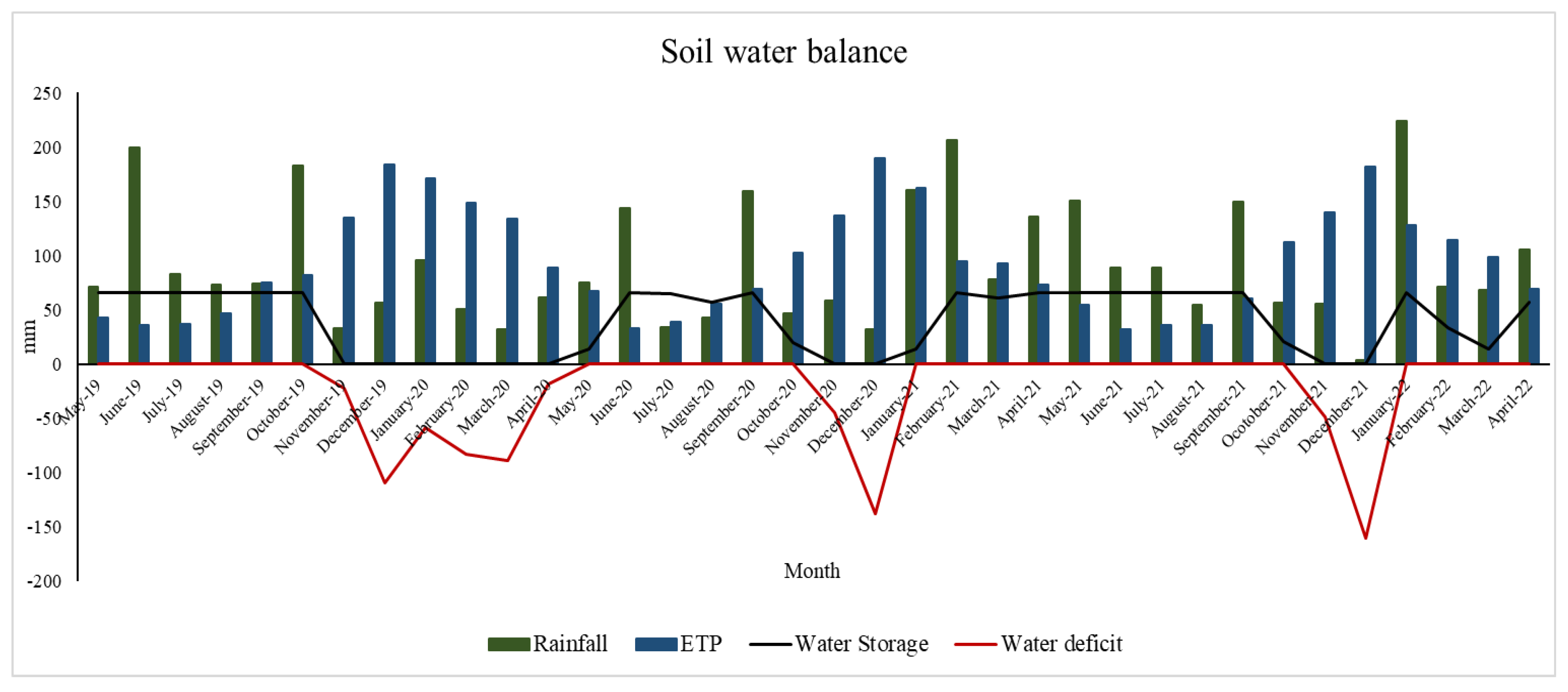
Soil water balance (
Figure 2) during the experimental period was characterized by a deficit between November and January (summer) in the three years. In Y1, the deficit was prolonged in time and covered the sowing period of pastures and crops in autumn (March and April). Soil water recharge occurred mainly in winter (June–September), when ETP was minimal, creating occasional muddy conditions in the grazing paddocks.
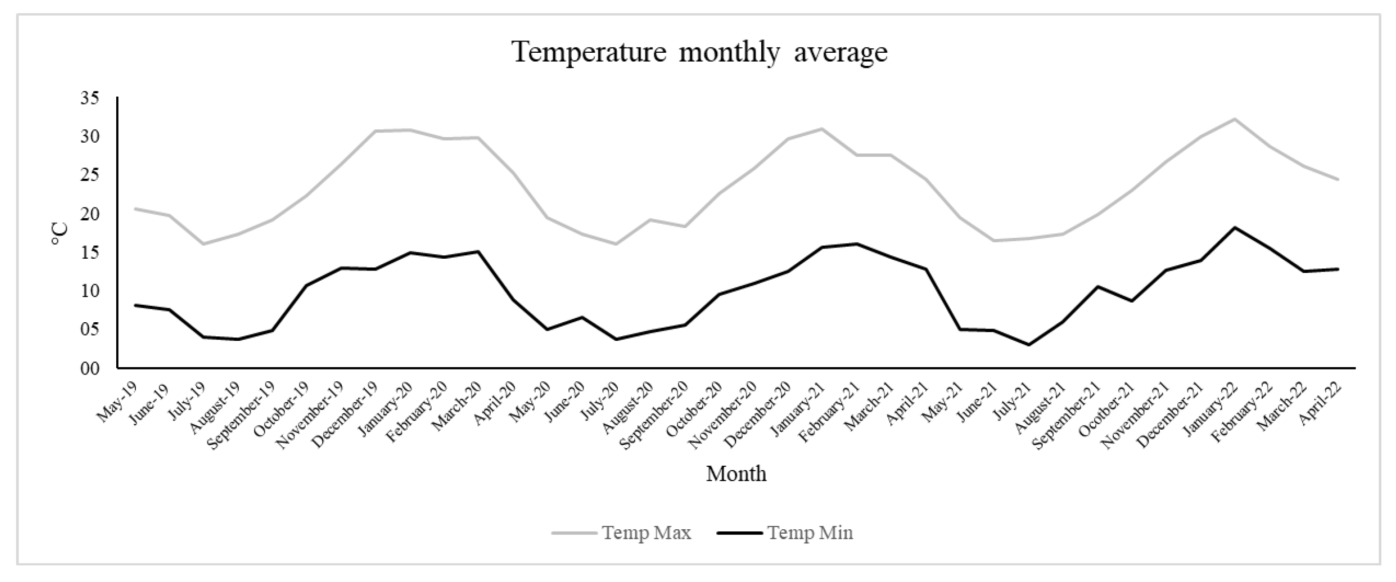
Figure 3 shows the monthly average of maximum and minimum temperatures (Ts). The maximum T was 41.4 °C and the minimum T was −5.1 °C, with a marked seasonal pattern. THI average was 62.1 ± 8.3. The maximum value was 81 and minimum was 41. During the experimental period, medium heat-stress conditions occurred on 6.1% of the days, whereas severe heat-stress conditions occurred on 0.8% of the days. These conditions were mainly in summer, where heat-stress conditions occurred on 16.2% of the days.
3.2. Crop Production
Table 4 shows grain yields for each crop in Year 1 (Y1, 2019–2020), Year 2 (Y2, 2020–2021) and Year 3 (Y3, 2021–2022) for the different rotations. Crop yield in CC was consistently lower than the yield obtained in crops rotating with perennial pastures (SR and LR). In Y1, grain yield reduction in CC was 36% (wheat), 11% (sorghum) and 17% (soybean) compared with the yield average observed in SR and LR. The same tendency was obtained in Y2 (10%, 8% and 15% yield reduction in CC for wheat, sorghum and soybean, respectively). During Y3, soybean grain yield in CC was 3% higher than the average of LR and SR. Due to adverse climatic conditions, oat crops were harvested only in Y2 and Y3 for SR and LR and Sorghum crops were not harvested in Y3.
Hay was produced in Y1, Y2 and Y3 from black oat paddocks (CC, SR and LR) and from one block of tall fescue (FR). Hay production (kg DM/ha) in Y1 was 50.1 in CC, 632.2 in SR, 90.1 in LR and 466.7 in FR, whereas in Y2, 916.7 was produced in CC, 417.8 in SR, 174,1 in LR and 458.3 in FR. During Y3, hay production was 516.7, 589.3, 276 and 441.6 in CC, SR, LR and FR, respectively.
3.3. Forage Growth
Data are presented as an average of different paddocks for oat, Italian ryegrass, natural grassland, permanent improvement and tall fescue, whereas in the permanent pasture, data are presented as an average of different ages in LR and SR (
Table 5).
In Y1, the white-clover-based permanent pasture (PP) in LR grew (kg DM/ha/day) 36.9 ± 28.03, 17.6 ± 15.26, 16.4 ± 8.60 and 14.8 ± 14.40, for first-, second-, third- and fourth-year pasture, respectively, and average daily growth decreased with the age of the pasture. In red-clover-based PP, maximum values were recorded in October (54.1 kg DM/ha/day) and minimum were in December and January (0 kg DM/ha/day). In both annual pastures (oat and ryegrass), maximum growth was registered in July (29.1 and 28.2 kg DM/ha/day, respectively). Tall fescue seeded in FR registered a maximum growth in October (57.2 kg DM/ha/day) and minimum growth in December (2.20 kg DM/ha/day). NG and PI had a marked peak of production in spring–summer, with maximum values registered during October–November (23.4 kg DM/ha/day) and minimum in June–July (0 kg DM/ha/day).
Similar forage growth results were obtained in Y2. Maximum values in PP were obtained in February (40.7 and 36.8 to LR and SR) and minimum values were observed in July (11.2 and 11.3 kg DM/ha/day). Maximum values in Oat and Ryegrass were recorded in September and August. In Tall Fescue, maximum values were observed in March (39.5 kg DM/ha/day). Finally, maximum values in NG and PI were observed in February–March (43.8 and 25.9 kg DM/ha/day).
During Y3, maximum values in PP were observed in September (106 kg DM/ha/day) and minimum values were observed in summer (0 kg DM/ha/day). In Oat and Ryegrass, maximum values were observed in May (56.1 kg DMD/ha/day) and August (39.2 kg DM/ha/day). Maximum values in NG were recorded in February, after a dry period, and the minimum values were observed during winter months and November and January. Maximum values in PI were obtained during March (43.5 kg DM/ha/day) and minimum values during June. In three years, Y1, Y2 and Y3, forage growth of summer crops (sorghum and moha) was estimated using values from the bibliography. Reference values were 100 kg DM/ha/day and 70 kg DM/ha/day for sorghum and moha, respectively [
47,
48].
3.4. Forage Production
Table 6 shows DM production for the four systems. Statistical differences were detected among systems. The highest productivity was observed in FR and SR, whereas the highest variability was observed in LR and SR. On the other hand, the lowest variability was observed in FR and CC (with the highest and the lowest DM production on average).
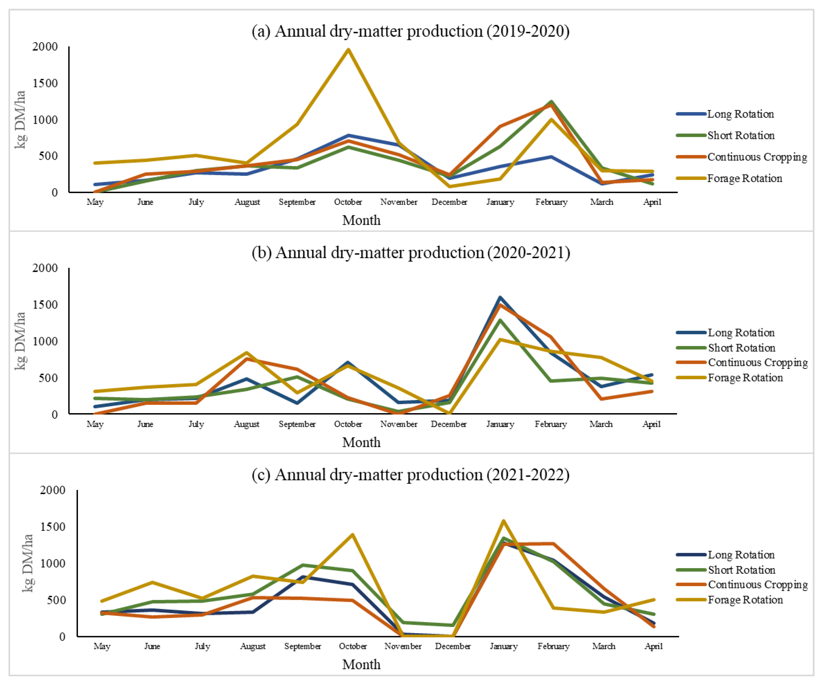
Forage production was higher in spring compared with the rest of the seasons (
Figure 4). The second forage production peak was registered in summer, associated with active growth of summer annual crops (sorghum and moha). Critical periods were observed in late spring (November–December) and early autumn (March–April), where systems had low DM production, associated with the presence of low-productive fallows, after glyphosate application, preparing the land for seeding first-year pastures (autumn) and annual crops (autumn and spring). The proportion of fallows within the PaCrR increases as the length of the pasture decreases, e.g., 100%, 75% and 50% of the area under the PaCrR corresponds to fallows in autumn for CC, SR and LR, respectively.
Established perennial pastures produced forage throughout the year. Species composition of perennial pastures determined the distribution of forage production. Pastures with white clover, tall fescue and birdsfoot trefoil in LR produced 26.3 ± 8.21% of the total annual DM production during winter, 34.8 ± 19.03% during spring, 23.4 ± 13.15% in summer and 15.5 ± 7.08% in autumn, averaging across Y1, Y2 and Y3. Short pastures in SR, comprising Yorkshire fog and red clover, had a more even distribution of forage production throughout the year compared with pastures in LR. They produced 23.9 ± 8.55%, 30.8 ± 14.43%, 28.1% ± 8.09% and 17.1 ± 10.33% of the total forage production in winter, spring, summer and autumn, respectively. Permanent improvement pasture in CC, which had a similar botanical composition to the pasture in LR, produced 16.2 ± 3.26% of the total DM production in winter, 41.5 ± 9.36% in spring, 21.1 ± 12.10% in summer and 21.2 ± 14.18% in autumn. Tall fescue in FR produced 38.6 ± 6.09% of the total annual DM production in winter, 34.3 ± 17.28% in spring, 19.8 ± 14.01% in summer and 7.3 ± 6.05% in autumn. Annual forage production of NG was 2947, 3811 and 3413 kg DM/ha for Y1, Y2 and Y3, respectively.
LR, SR and CC include pastures with legumes in a proportion of 48, 43 and 33% of the total area of the system, respectively. In LR, DM legume production was 39.5 ± 24.25%, 14.3 ± 14.01%, 17.2 ± 13.09% and 4.91 ± 2.079% of the total DM production for the 1st, 2nd, 3rd and 4th year of pasture, respectively. In SR, legumes contributed to 39.7 ± 28.22% and 21.5 ± 11.25% of the total DM (1st and 2nd year of pasture, respectively). The PI in CR had a legume contribution of 8.2 ± 5.35% of total DM production, averaging across Y1, Y2 and Y3. Data about forage quality are detailed in
Supplementary Materials (
Tables S1–S3).
Total nitrogen contribution to the soil is presented in
Figure 5. Data are presented as an average across Y1 (2019–2020), Y2 (2020–2021) and Y3 (2021–2022) for each pasture, according to age of pasture (1st year, 2nd year, 3rd year and 4th year). There was a trend to decrease N fixed as pasture age increased in both pastures (LR and SR).
3.5. Supplementation
Animals from all the systems received strategic supplementation when the available forage was not enough to prevent LW losses from the animals. Levels of supplementation are presented as kg feed DM/ha (
Table 7). In all years, supplementation was carried out during winter. In addition, summer supplementation was carried out in Y2 and Y3 associated with a prolonged dry period.
3.6. Grazing Management
Table 8 shows percentages of pasture occupation for each system. On average, pastures outside the area of the PaCrR were occupied by animals 45.1%, 40.2% and 40.7% of the time in Y1, Y2 and Y3, respectively. The combined use of NG and PI in CC had the maximum occupation rate (75.1% and 64.1% and 58.6%, respectively), whereas NG in FR had the minimum occupation rate (21.1%, 26.6% and 21.9%, respectively).
Within PaCrR, PP had an average occupation of 52.3%, 51.5% and 47.4% in Y1, Y2 and Y3, respectively. In both years, PP in FR had the highest occupation rate due to the absence of annual forage crops. LR and SR had similar occupation rates for PP. On average, each grazing period in PP lasted 6.2, 7.5 and 4.4 days in Y1, Y2 and Y3, respectively, whereas each grazing event in the annual forage crops lasted 4.3, 3.2 and 6.6 days in Y1, Y2 and Y3, respectively.
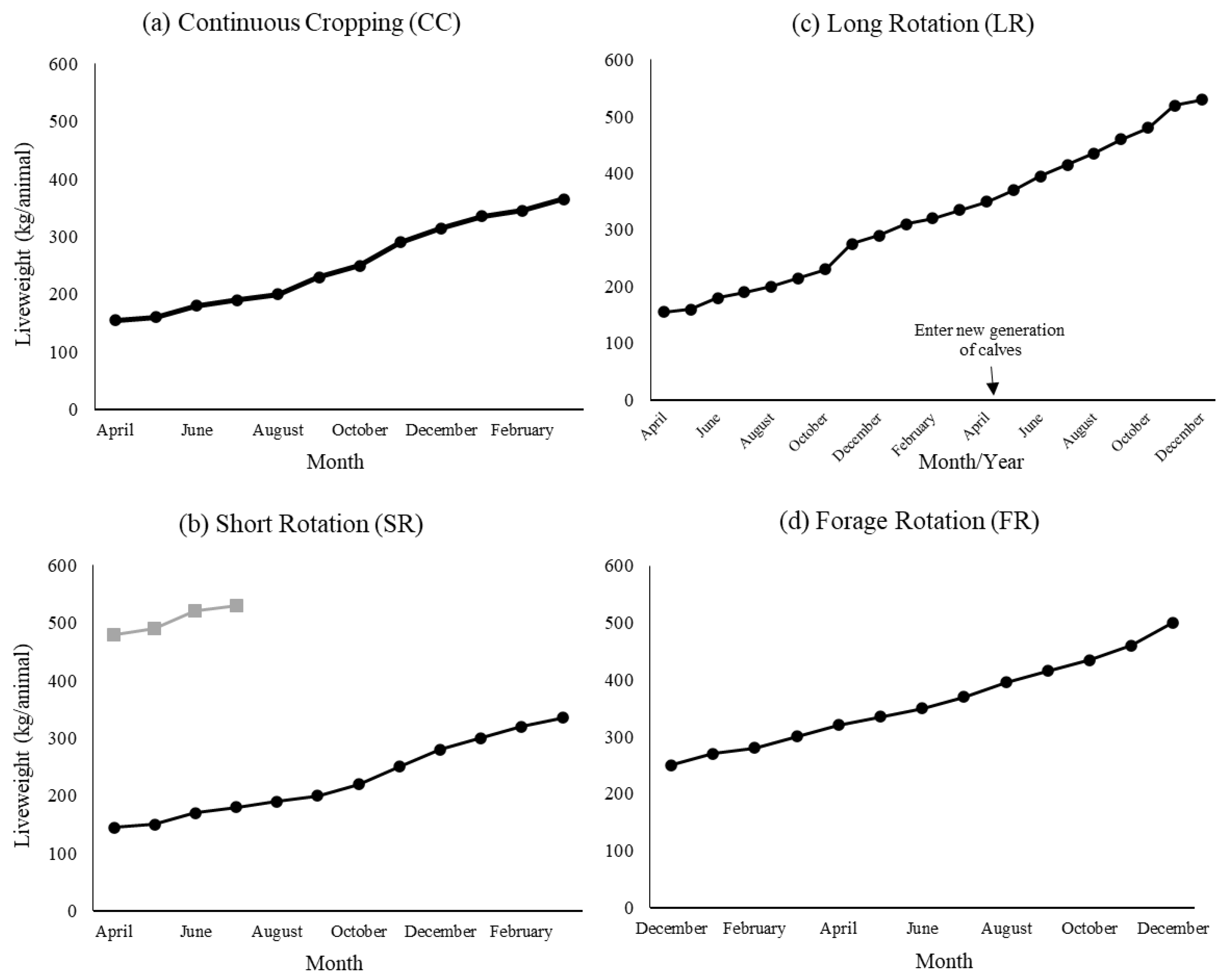
3.7. Animal Performance
Table 9 shows seasonal average daily gain (ADG) for the different livestock categories. The highest and lowest individual ADG was observed in spring and winter, respectively. Animal categories closer to slaughter (finishing steers and cows) registered numerically higher ADG compared to rearing categories (calves). However, younger animals (<18 months old) registered a better efficiency (lower numeric values) than older animals. On average, growing categories (calves and heifers) required 46.2% and 25.9% less feed to gain 1 kg of LW than culled cows and finishing steers, respectively.
Efficiency in each system was calculated from F/G ratio (
Table 10), considering the proportion of kg of LW produced in each system according to each animal category. Although no significant differences were found, a tendency to obtain better efficiencies was observed in those systems with a higher proportion of rearing. Forage utilization varied between 50 and 60% in LR, 55 and 62% in SR, 48 and 52% in CC and 35 and 39% in FR.
Average animal stocking rate (±s.d.) during the 3 years was 614 ± 33 (CC), 600 ± 44 (SR), 575 ± 15 (LR) and 498 ± 23 (FR) kg LW/ha. The minimum and maximum stocking rates were registered in FR (Y2: 473 kg LW/ha) and CC (Y3: 648 kg LW/ha), respectively.
Overall, CC and SR were the systems with the highest LW production and lowest variability over the years (
Table 11). CC and SR achieved the highest annual LW production in Y1 (404 and 393 kg LW/ha/year, respectively), Y2 (438 and 444 kg LW/ha/year, respectively) and Y3 (437 and 418 kg LW/ha/year). On the other hand, FR was the system with the lowest LW production in the three years (307, 344 and 280 kg LW/ha/year, Y1, Y2 and Y3, respectively), whereas LR achieved an intermediate level of production (316, 394 and 399 kg LW/ha/year, Y1, Y2 and Y3, respectively). In all systems, spring was the season with the highest contribution to the total LW production (35–48% in Y1, 38–46% in Y2 and 29–49% in Y3), while autumn had the lowest contribution (6–7% in Y1, 3–17% in Y2 and 8–22% in Y3).
In CC and FR, 100% of the annual LW production per ha was obtained from rearing calves and finishing steers, respectively. Both stages of production were carried out in LR, contributing to 57% (rearing calves) and 43% (finishing steers) of the total annual LW production averaging over the years. In SR, rearing heifers was the main contributor to the total LW production (92%), followed by finishing cows (8%).
4. Discussion
Integrated Crop Livestock Systems allow one to improve food production while, at the same time, reducing negative environmental impacts and, therefore, are an option to achieve economic, sociological, ecological, energy, environmental and biogeochemical synergies and efficiencies [
49]. The four systems evaluated in this work present different intensities of soil use and, at the same time, each system has a specific associated livestock strategy. The concept behind this rotation–livestock differential strategy association is that those systems that feature more intensive soil use, with more use of inputs (e.g., fertilizers, fuel, herbicides), are associated with more efficient livestock strategies (e.g., less feed to gain ratio, less GHG emissions), whereas systems with less intensity of soil use, including pasture phase in their rotation, are associated with less efficient livestock strategies evaluated (e.g., finishing animals), presenting trade-off to reduce negative impacts of agriculture or livestock production [
31].
This work reports results of productivity and management from four ICLSs for three years and aimed to characterize the systems according to crop production (t/ha); forage growth (kg DM/ha/day); forage production (kg DM/ha); and N fixation (kg N/ha) from legume production. Further, results about animal and system performance, such as liveweight production, liveweight gain, stocking rate and feed to gain ratio, were presented. Regarding management, supplementation data (kg DM/ha), fertilization (kg/ha) and pasture occupation were presented with the objective to understand how systems work.
Liveweight production (LWP, kg LW/ha/year) varied among systems. In general, CC and SR, i.e., those systems that included rearing stock in high proportion, had more LWP than LR and FR, which are associated with finishing cattle. This can be explained by the different biological efficiency of each stage, i.e., rearing vs. finishing [
50]. This is evidenced by the differences in F/G ratio among systems, with CC and SR requiring, on average, 17.3% less kg of DM forage per each kg of LW produced. These LWP levels were similar to those reported by Terra and García-Préchac (1996–2000) [
51] and Pereyra (2013–2017) [
52], in the same experimental site on permanent pastures and annual grazing crops, without support area.
There were differences in LWP across years. Y1 had the lowest levels of production associated with climatic conditions that made seeding of pastures difficult (autumn–early winter), along with the fact that Y1 could be considered as a management adjustment year. Year two had higher levels of meat production than Y1, explained by a greater number of animals in CC and SR and higher levels of supplementation in LR and FR (in this system with fewer animals than Y1). During Y3, levels of production were similar to Y2 in CC (−1 kg LWP/ha) and LR (+5 kg LWP/ha), whereas in SR and FR, levels of production were reduced (−26 kg LWP/ha and −34 kg LWP/ha, respectively). Although DM production was higher in Y3 than Y1 and Y2, dry conditions and high temperatures during summer, which affected forage production and quality and determined heat-stress conditions to animals, could explain the reduction in LWP.
Strategic supplementation played an important role in systems, improving LWP. This effect was observed mostly in those systems with lower efficiency (finishing animals), where the use of supplements was the highest on average (LR) or low but with high impact, improving LWP (FR). This allows one to infer a certain dependency on supplementation in these systems compared with those that achieved higher levels of LWP with lower levels of supplement.
Autumn and winter were critical periods for liveweight gain (LWG, kg/ha/day), associated with fallows, seeding of pastures, high water content and low DM forage mass in pastures. The highest LWGs were observed during spring, explained by a peak of DM production and improvements in climatic conditions. This determined the moment when the most kg of liveweight was produced along the year and the moment when animals were ready to slaughter.
DM production had slight differences among years, despite variation in climatic conditions among years. These conditions affected the seasonal productivity and the intra-annual distribution more than the annual total production of DM. Further, FR and SR had the highest production on average. High levels of nitrogen fertilization in FR and the absence of fallow periods and growth rates of permanent pasture in SR could explain these results. However, dry conditions during summer strongly affected tall fescue in FR production and quality and gave rise to weed growth (mainly Cynodon dactylon).
Natural grassland is a key component in ICLSs and had a strategic use during adverse conditions, as a supporting area. These grasslands are mostly composed of C4 grasses with high DM production in spring–summer [
53]. On the other hand, permanent pastures had high DM production in winter–spring, which allowed for complementary use of both grassland types and avoided overgrazing during critical periods for NG. Occupation of NG was different between systems; the highest occupation was in CC and SR. These systems with a short and without-pasture phase, respectively, had an important proportion of area in fallow period in autumn and spring (75% and 100% of area in rotation, respectively), which explained most of the use of NG, due to a reduction in the improved area. At the same time, these systems had low stocking rate during autumn, when grazing area is reduced. The use of permanent pastures was predominant in LR and FR and NG use was less than that for CC and SR.
Grain production varied among systems and there was a substantial effect of the pasture phase in grain yields. In Y1 and Y2, CC had less grain production than SR and LR. During Y3, CC had soybean production with similar values to LR. Along these lines, various authors report that the inclusion of pastures in a rotation with crops promotes better soil quality, associated with higher SOC, than those that do not include pastures [
54]. Results presented by Terra and Macedo [
55] showed that, in the same experiment, between 1995 and 2005, CC had significantly lower SOC than systems that rotated with pastures (i.e., LR and SR). Similarly, it has been reported that Brazilian ICLSs, with grazing animals, allow one to improve grain yield after the pasture phase, due to improved soil properties, i.e., soil microbial (mass, diversity) and soil structure (composition, density, porosity, nutrients) [
56].
Climatic conditions (wet conditions in winter and dry conditions in summer) affected oat grain production in Y1 and sorghum grain and wheat grain production in Y3, respectively, which allowed us to only obtain by-products that were used as fibrous feed in livestock production. Although grain production in the current scheme of production is considered as an output of the systems, in some cases, it could be considered as an input to LWP (to feed animals), depending on variation in international prices, environmental conditions and the needs of each system. This flexibility in resource use is presented as an advantage in ICLS management.
Legume inclusion in the rotation supplied nitrogen to the system. Pasture phase fixed 27.8 ± 2.59 kg N per ha/year in LR, 52 ± 45.2 kg/ha/year in SR and 10.8 ± 7.42 in CC, on average. These values had high variability, depending on the age of pasture, driven by botanical composition and year, though represented an important contribution given the current fertilizer prices. Further, biological fixation of nitrogen is more efficient in terms of GHG emissions and energy use than N inputs from inorganic fertilizers, with similar values of losses to waterways [
57]. Moreover, sowing legumes with high levels of condensed tannins, e.g.,
L. corniculatus L., as conducted in the permanent pasture of LR and permanent improvement in CC, is a way of reducing emissions per kg of DM consumed [
58] and reducing N losses through leaching [
59].
Livestock production contributes nutrients through excreta. Russelle et al. [
24] highlighted the importance of manure use to reduce costs and improve soil fertility. In Palo a Pique LTE, excreta are distributed homogenously within the boundaries of the systems, due to rotational stocking with a few days of permanence in each paddock and high stocking density. According to Ward et al. [
25], N fixation and livestock excreta allow for nutrient cycling. These authors discuss the importance of the circularity of nutrients in livestock systems, associated with lower costs of production and lower environmental impacts. In this regard, Moraes et al. [
56] reported that recycling of nutrients in the livestock phase is influenced by stocking rate and, in consequence, these systems export less nutrients out of the system than the crop phase.
Ruminant livestock can produce human food from human-inedible feedstuffs [
19]. In the four systems evaluated, livestock played an important role by transforming grass into high-quality protein, i.e., kg of meat. The pasture phase allows one to produce feed for animals in marginal soils, where continuous cropping is unsustainable [
31] and, at the same time, the use of high-quality pastures allows for improved liveweight production. The use of human-edible grains to feed animals is minimum, reducing the competition for resources [
60].
Although the systems analyzed here lacked spatial replication because of the large-scale and multidisciplinary crop–livestock research approach, we presented three years of data that were considered as a replication in time. The main objective is to report the real results and coefficients from mixed livestock systems in Uruguay. In this regard, Murison and Scott [
61] reported several published studies that used unreplicated treatments related to grazing livestock. They concluded that while treatments need to be replicated to allow for measurement of the experiment error, there are circumstances where appropriate scale may have priority over replication. On the other hand, the same authors reported the importance of assessing the whole-farm effects, emergent properties of the systems and, at the same time, individual productivity.
ICLSs present some opportunities related to international prices of commodities. However, there are also challenges, namely: (i) the dependence of external inputs to maintain high DM production in a scenario of price variability (i.e., fertilizer use); (ii) environmental issues associated with the need to reduce emissions per unit of product while maintaining high levels of production over time without wasting resources (i.e., forage quality and productivity, grazing management and C sequestration in soils, particularly in CC, where the rotation did not include a pasture phase); (iii) the need to adapt this kind of system through technologies to reduce the impact of climate change (i.e., diversification of forage basis in FR); (iv) the necessity to improve productivity, particularly in those systems that did not reach the proposed production levels (FR and LR), without increasing the use of human-edible food to feed animals (i.e., through improved forage utilization).


