Abstract
Utilizing degraded quality waters such as saline water as irrigation water with proper management methods such as leaching application is a potential answer to water scarcity in agricultural systems. Leaching application requires understanding the relationship between the amount of irrigation water and its quality with the dynamic of salts in the soil. The HYDRUS-1D model can simulate the dynamic of soil salinity under saline water irrigation conditions. However, these simulations are subject to uncertainty. A study was conducted to assess the uncertainty of the HYDRUS-1D model parameters and outputs to simulate the dynamic of salts under saline water irrigation conditions using the Markov Chain Monte Carlo (MCMC) based Metropolis-Hastings algorithm in the R-Studio environment. Results indicated a low level of uncertainty in parameters related to the advection term (water movement simulation) and water stress reduction function for root water uptake in the solute transport process. However, a higher level of uncertainty was detected for dispersivity and diffusivity parameters, possibly because of the study’s scale or some error in initial or boundary conditions. The model output (predictive) uncertainty showed a high uncertainty in dry periods compared to wet periods (under irrigation or rainfall). The uncertainty in model parameters was the primary source of total uncertainty in model predictions. The implementation of the Metropolis-Hastings algorithm for the HYDRUS-1D was able to conveniently estimate the residual water content (θr) value for the water simulation processes. The model’s performance in simulating soil water content and soil water electrical conductivity (ECsw) was good when tested with the 50% quantile of the posterior distribution of the parameters. Uncertainty assessment in this study revealed the effectiveness of the Metropolis-Hastings algorithm in exploring uncertainty aspects of the HYDRUS-1D model for reproducing soil salinity dynamics under saline water irrigation at a field scale.
1. Introduction
The severity of water shortage for irrigated agriculture is becoming a global catastrophe. On the other hand, the sustainability of agricultural systems and water resources has been extremely challenging due to the rising competition in water demands of the agricultural, industrial, and municipal sectors [1]. Irrigation with saline waters could be a proper alternative to freshwater to sustain the agricultural industry in arid and semi-arid regions facing different water scarcity levels [2]. These waters are mainly obtained from agricultural drainage water, municipal wastewater, and low-quality groundwater. It has been indicated in several studies that when saline water is used for irrigation purposes, special focus should be considered on controlling salinity accumulation in the crops’ root zone to achieve long-term productivity in the region [3,4,5,6]. The unsuitable management of saline water irrigation can potentially restrict crop water and nutrient uptake due to the inducing salinity build-up in the soil [7]. The salinity distribution and its levels depend on interactions of irrigation, rainfall, evapotranspiration, and the drainage condition of the agricultural fields [8]. Thus, implementing an effective method to alleviate concentrated salinity in the crops’ root zone is crucial. Leaching excessive salts downward from crops’ root zone through the application of more water than the crops’ water requirement during the growing season has been an effective method for salinity control. Leaching application is a critical factor in managing soil-soluble salts brought by saline water irrigation [9]. Therefore, balanced management between applying extra water to control salinity and conserving groundwater resources due to additional water withdrawal is expected. The ratio of water that passes the root zone to the amount of irrigation water is called the leaching fraction (LF) [9]. The minimum leaching fraction of irrigation water with particular quality that needs to be applied over the growing season to keep soil salinity below the crops’ salinity thresholds is called the leaching requirement (LR) [10]. To determine the correct value of LR, steady-state and transient-state are two existing approaches and introduced methods in the literature. In steady-state analysis, specific assumptions have been made that include the continuous downward flowing of irrigation water at a constant rate, constant evapotranspiration rate during the growing season, and constant soil soluble salt concentration at any point [8,11]. Comparing field observations proves that none of these assumptions are realistic [8,11]. Thus, using transient-state methods is preferable to compute suitable LR values when the source of irrigation water is saline. One of the well-distinguished transient numerical models is the HYDRUS-1D, model which has the capability of simulating water flow and transport of solutes and ions in unsaturated conditions of soils [12]. The HYDRUS-1D along with its solute transport and root water uptake modules have been proven to be a reliable model for investigating management scenarios regarding long-term and short-term effects of using marginal quality waters as irrigation water on soil salinity and water content [13,14]. Gonçalves et al., 2006 have shown that the HYDRUS-1D model successfully simulated soil water content, overall salinity, and soluble ions over and out of the irrigation season. The model was able to reasonably describe the contribution of rainfall in leaching soluble salts deposited by irrigation during the season [15]. Noshadi et al., 2020 used soil column lysimeters to calibrate and validate the HYDRUS-1D model under different controlled groundwater depths. They revealed that statistical indices of normalized root mean square error (NRMSE) and degree of agreement (d) values were 9.6% and 0.64 for simulating soil water content, and 6.2% and 0.98 for simulating soil salinity, respectively [16]. It has been shown by Phogat et al., 2010 that the HYDRUS-1D predictions of water percolation and soil electrical conductivity of sandy loam soil in mini lysimeters study were not statistically different from the measurements [17]. Salma et al., 2019 have investigated the reliability of the HYDRUS-1D model in terms of investigating the effects of different irrigation regimes, including full and deficit irrigation, on root water uptake and root zone salinity. Their results indicated good accuracy of the model by achieving the root mean square error (RMSE) values of 0.008 m3 m−3 and 0.28 dS/m for simulating soil water content and soil water electrical conductivity (ECsw), respectively [18]. Liu et al., 2019 calibrated and validated the HYDRUS-1D model to investigate the soil salt dynamic of the winter wheat–summer maize root zone irrigated with brackish water in a semi-arid region. The results have shown the model’s good performance regarding soil water content (SWC) and ECsw simulations. The RMSEs for simulating SWC and Ecsw were in the range of 0.017–0.04 cm3 cm−3 and 0.059–0.069 dS/m, respectively. In addition, the coefficient of determination (R2) values were from 0.78 to 0.92 for SWC simulations and from 0.67 to 0.89 for Ecsw simulations [19]. Helalia et al., 2021 have simulated water use and soil salinity of drip-irrigated almond and pistachios root zones by the HYDRUS-1D model under different irrigation water salinities for multiple locations in San Joaquin Valley (SJV), California. Their results have shown good accuracy of the model as NRMSE values between simulated and measured volumetric water content varied from 0.033 to 0.28. Moreover, the coefficient of correlation (R) values varied from 0.4 to 0.72 for ECsw, showing erratic behavior of the model in different locations due to multiple factors such as the non-uniformity of root and water redistributions under drip irrigation [20]. A challenge to obtaining acceptable outputs of the model is the calibration of its parameters, which is usually time and money consuming. Inverse modeling has been known as a convenient technique for calibrating HYDRUS-1D based on observational data [21,22,23,24]. Nevertheless, estimating model parameters are still associated with uncertainties that are reflected in model outputs. To achieve valid results from the model, it is necessary to quantify this type of uncertainty [25]. To date, very few studies have explored the uncertainty analysis of HYDRUS-1D parameters, particularly for simulating the salinity dynamic of the soil under saline irrigation conditions [26,27,28]. This study, by pursuing the Bayesian theorem, investigates the conditional probability distribution of the HYDRUS-1D parameters, grounded on the measurements. The Bayesian theorem consists of three main terms: (a) the likelihood function that incorporates the model outputs and measurements to identify the errors, (b) prior probability that covers all of the uncertainty without considering measurements (initial information), and (c) the posterior probability that combines the previous knowledge (prior) and new information (likelihood) to gain uncertainty of the model [29,30]. Various methods have been implemented to determine the uncertainty analysis of the models based on Bayesian inferences. Among these methods, those based on Markov Chain Monte Carlo (MCMC) approach have gained significant popularity in studies, particularly in hydrology [31,32,33,34,35,36]. The MCMC has been built based on formal Bayesian inference concepts to estimate the models’ parameters and quantification of uncertainty. The MCMC creates a Markov chain whose target distribution is posterior distribution. The Markov chain illustrates the sampling design for simulating Monte Carlo [34,37]. Kunnath-Poovakka et al., 2021 have investigated the parameters’ uncertainty of a hydrological model known as the Australian Water Resource Assessment Landscape (AWRA-L) model using an MCMC method and incorporating remotely sensed evapotranspiration and soil moisture data [38]. Yang et al., 2020 have taken advantage of the MCMC approach to develop a method for drought risk assessment under uncertainty [39]. Xu et al., 2018 adopted an MCMC-based algorithm to estimate the parameters and uncertainty of two-parameter non-stationary Lognormal distribution to analyze flood frequency in a river basin [40]. So far, most of the attention has been on implementing these Bayesian theorem-based methods for hydrological problems and few studies have been accomplished to use these approaches for addressing problems in irrigation science. The main aim of this study is to couple a Bayesian MCMC algorithm known as Metropolis-Hastings (M-H) with the numerical model of HYDRUS-1D to quantify the uncertainty of the parameters of water flow, solute transport, and root water uptake modules of the model for simulating soil salinity dynamics over the growing season and out of the growing season in under field conditions.
2. Materials and Methods
2.1. Site Description and Experimental Data
The field experiments were conducted in Alvalade do Sado, Alentejo, Portugal [15]. Soil monoliths were built for the aims of the study. The monoliths had 1.2 m2 × 1.00 m deep dimensions, which were isolated by plastic to restrict the lateral seepage of water and solute. The soil surface was exposed to atmospheric conditions, and the bottom had free drainage conditions. The vegetation cover was annual spontaneous plants such as gramineous, leguminosae, and compositae. To measure soil water content and pore ware salinity, TDR probes using waveguides from the Trase System (Soil Moisture Equipment Corp., Goleta, CA, USA) and ceramic suction cups were installed at 10, 30, 50, and 70 cm, respectively. The electrical conductivity (EC) of extracted water, using ceramic suction cups, was analyzed as soil water salinity (ECsw). The experiments were conducted for two growing years (505 days), starting on 15 May 2003, to 30 September 2004. The first irrigation season was started on 29 May 2003 and ended on 20 August 2003. The irrigation events of the next growing season were initiated on 23 June 2004 and continued until 20 August 2004. The monoliths were exposed to atmospheric conditions for the days out of irrigation seasons. It should be mentioned that no rainfall occurred from 21 August 2003 until 1 November 2003, and just one rainfall occurred from 21 August 2004 until 30 September 2004. The crop’s daily evapotranspiration and precipitations during the experiments are presented in Figure 1, and the irrigation seasons are specified with orange bars.
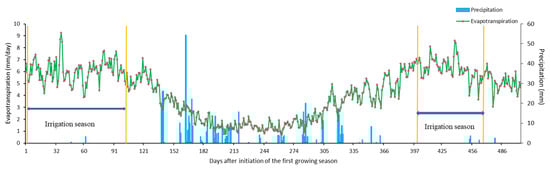
Figure 1.
The daily crop evapotranspiration and the precipitations during the experiments starting on 29 May 2003 until 30 September 2004. Orange bars are indicators of irrigation seasons.
In addition, Table 1 shows the average values of weather variables for the study period. The electrical conductivity of irrigation water (ECiw) was 1.6 dS/m (Table 2). Irrigation scheduling followed a fixed 10 mm irrigation depth for each irrigation event during the growing season. The soil profile was refilled whenever the depletion of total soil water reached 10 mm based on soil water content readings. Therefore, variable irrigation intervals were pursued in this study. The monoliths were irrigated using a surface irrigation method similar to the basin irrigation system [15]. The amount of seasonal irrigation depth was 500 mm for each growing season. The total amount of rainfall was 323.8 mm, and 170.1 mm for our experimental period in 2003 and 2004.

Table 1.
The average values of the weather parameters for study period in 2003 and 2004 near Alvalade do Sado, Alentejo, Portugal.
Table 2.
Chemical characteristics of the irrigation water [15].
The soil texture was silty loam from the soil surface to 85 cm depth and loam from 85 cm to 170 cm soil depth. The physical and chemical characteristics of the soil obtained through laboratory analysis including are presented in Table 3.
Table 3.
The physical and chemical characteristics of the soil [15].
In addition, the initial chemical conditions and the volumetric soil water content of the soil profile of the monoliths are presented in Table 4. As it has been shown, the average soil water salinity (ECsw), soil water content (θv), and sodium adsorption ratio (SAR) were 0.6 dS/m, 0.276 cm3 cm−3, and 1.92 (mmol(c)L−1)0.5, respectively.
Table 4.
The initial conditions of the soil profile of the monoliths [15].
The meteorological data were obtained from the weather station located 10 m from the experimental field and the Penman-Monteith method, Allen et al., 1998 was used to calculate the daily evapotranspiration [41]. To conduct ET partitioning for evaporation and transpiration, the average leaf area index (3.5 m2 m−2) and its corresponding soil cover factor (SCF) were used.
More details concerning experimental setup and study conditions can be found in Gonçalves et al., 2006.
2.2. HYDRUS-1D Model Simulations
The simulations were accomplished for the first 100 cm of the soil profile where the monoliths were built to prevent lateral water flow.
2.2.1. Water Flow and Root Water Uptake Modeling
The HYDRUS-1D model simulates water flow in the soil under saturated and unsaturated conditions by numerically solving the Richards equation (Equation (1)) using the Galerkin finite element method:
where θ is volumetric water content (L3 L−3), h is suction head (L), t is time (T), z is vertical coordinates (L), K(h) is soil unsaturated hydraulic conductivity (L T−1), and S(z,t) is sink term known as root water uptake (L3 L−3 T−1).
The relationship between h and θ is described by the Van Genuchten-Mualem function (Equation (2)) as follows [42]:
where θs is the saturated soil volumetric water content (L3 L−3), θr is the residual soil volumetric water content (L3 L−3), and α, n, and m are empirical parameters (m = 1 − 1/n).
The unsaturated hydraulic conductivity (Equation (3)) is described as a function of h [42]:
where Ks is the saturated hydraulic conductivity (L T−1), l is the empirical parameter, and Se is the effective saturation (Se = (θ − θr)/(θs − θr)).
The root water uptake or the sink term in Richards’ equation (Equation (1)). It represents the volume of water removed by plants’ roots (Equation (4)) from the unit of soil per time unit [43]:
where S(z) is the sink term in Richard’s equation (L3 L−3 T−1), β(z) is the normalized root density distribution (L−1), Tp is the potential transpiration rate (L3 L−2 T−1), α(h,π) is the dimensionless root water and salinity stresses response function.
The normalized linear root density distribution function (Equation (5)) based on root depth is as follows:
where z is root depth (L). Based on the observations in this study, 80% of root density was distributed in the first 30 cm of soil root zone, and the remaining 20% root density was extended to 70 cm soil depth [15].
The combined water and salinity stress response function is as follows [43,44]:
where h is the soil water pressure head (L), b is the slope of water uptake reduction as a function of the average root zone salinity (-), and a is the threshold of plant root water uptake to average root zone salinity (dS/m), π is root zone average salinity (dS/m), and P1 and h50 (L) are empirical crops, soil, and climate-based parameters. The h50 is known as the water pressure head, which reduces the root water uptake by half [44].
The partitioning of evaporation and potential transpiration can be computed by application of Beers’ law (Equation (7)) to calculate potential evapotranspiration as follows [45]:
where ETp is potential evapotranspiration (L T−1), and k is the dimensionless coefficient of radiation attenuation which was considered equal to 0.4 [14,46,47].
2.2.2. Solute Transport Modeling
The advection-dispersion equation was solved numerically in HYDRUS-1D as follows [48]:
where θ is the volumetric soil water content, c is the solute concentration (M L−3), qw is the soil water flux (L3 L−2 T−1), z is the soil depth (L), and De is the effective dispersion coefficient [L2 T−1].
The effective dispersion coefficient is the combination of diffusion and dispersion coefficients [48]:
where is the effective diffusion coefficient [L2 T−1] and Dlh is the coefficient of hydrodynamic dispersion [L2 T−1].
where λ is a proportionality constant called dispersity [L] and v is the average pore water velocity [L T−1]. The v is obtained from the results of water flow flux [L3 L−2 T−1].
where θ is the volumetric soil water content, θs is the volumetric saturated soil water content, and is the diffusion coefficient in free water.
where l is known as the tortuosity factor (l).
2.3. The HYDRUS-1D Model Setup
The simulations of soil salinity dynamics have been conducted by the HYDRUS-1D model for soil profile 100 cm in the monoliths. As the soil texture was relatively uniform (Table 3) for the observational points at 10, 30, 50, and 70 cm soil depths, the soil material and layer were considered equal to 1. The simulations were conducted on a daily basis for 505 days (from 15 May 2003 to 30 September 2004). To perform the water flow simulation and describe the unsaturated soil hydraulic properties, the Van Genuchten-Mualem (Equations (1) and (2)) hydraulic model was chosen. The initial values of the water flow parameters for calibration and uncertainty purposes were determined by the default values in the HYDRUS-1D library for the silt loam soil. The atmospheric boundary condition with the surface layer was chosen to represent the study condition at the soil surface. The atmospheric boundary condition was determined using time series irrigation, precipitation, evaporation, and transpiration fluxes. The free drainage boundary condition was used for the bottom of the soil profile. The soil adsorption was negligible based on the field observations [15]. Thus, the adsorption was eliminated by selecting the linear equilibrium adsorption model and assigning the zero value to the distribution coefficient [48]. The upper and bottom boundary conditions for the Advection-Dispersion equation (Equation (8)) were concentration flux and zero concentration, respectively. The root water uptake simulations were carried out by the S-Shape [49] model, and simultaneously the slope and threshold salinity stress reduction function was taken into account in a multiplicative approach (Equation (6)). Moreover, the initial condition was determined by the soil water content and ECsw measurements at 10, 30, 50, and 70 cm as presented in Table 4.
To benefit from two years of observational data, the uncertainty analysis was undertaken for the first year of the study: 15 May 2003 to 22 June 2004, which included the growing season and out of growing season period. The outputs of the M-H algorithm as calibration results were validated for simulating ECsw and soil water content in long-term aspect, with continues observational data from 15 May 2003 until 30 September 2004. The simulations were carried out for the period of the beginning of the first growing season until 45 days after end of the second growing season in the validation process.
2.4. Uncertainty Analysis and Metropolis-Hastings
The term uncertainty has been defined as the degree of confidence in the decision-making process based on the target outputs from the models [25]. The Bayesian inference is convenient in terms of predicting the models’ parameters (posterior distribution) by operating the uncertainty analysis grounded on previous knowledge regarding the model parameters (prior distribution), observational data, and likelihood function. The Bayesian concept or inference is demonstrated as follows:
where θ is the parameter, Y is the observational data, P(θ|Y) is the posterior distribution, L(θ|Y) is the likelihood function, and P(θ) is the prior distribution. The likelihood is computed from the probability distribution of residuals between observations (Y). The residuals are frequently assumed uncorrelated, normally distributed, and independent [50]. Thus, the outcoming likelihood function is as follows:
where σ is the standard deviation of model errors, Yi is the observational data, and Yi(θ) is the model output. To gain more numerical stability and simplicity, the logarithmic form of the likelihood function was used in this study:
To conduct an uncertainty analysis of the HYDRUS-1D model for simulating solute transport under saline irrigation conditions, we used the posterior distribution of the following parameters:
Water flow parameters = [θr, θs, α, Ks, n, l];
Solute transport parameters = [λ, Dlw];
Salinity Stress for root water uptake = [a,b];
Water Stress for root water uptake = [h50,P1].
The uncertainty analysis was performed in the Bayesian framework using the Metropolis-Hastings (M-H) algorithm for the Markov Chain Monte Carlo method combined with Gibbs sampling. To execute the M-H algorithm, the initial step is identifying the proposal distribution to generate new parametric candidates. In this study, we assumed the priors to be uniformly distributed [51] over space, to assign the same probability to all possible values of parameters. Hence, uniform distribution was considered as the proposal distribution to generate the samples using the Monte Carlo approach. Therefore, the Metropolis-Hastings algorithm was applied as follows [52]:
- 1.
- Determine the length of the Markov Chain, T
- 2.
- Draw an arbitrary initial candidate (θi)
- 3.
- Calculate the proposed initial candidate density: P(θi|Y) = L(θi|Y)*P(θi)
- 4.
- For n = 2, …, T do:
- 5.
- Generate a candidate (θt) from proposal distribution (q(θ)).
- 6.
- Calculate the target density: P(θt|Y) = L(θt|Y)*P(θt)
- 7.
- Calculate the Random Walk Metropolis acceptance criteria:
- 8.
- Generate a random sample from the uniform distribution as U(0,1);
- 9.
- If U ≤ α then θn = θt;
- 10.
- Else θn = θt−1;
- 11.
- End of the loop.
To achieve the goals of the study, the M-H algorithm was implemented in R-Studio V 1.4.1717 (Posit Corp, Boston, MA, USA) environment for the HYDRUS-1D model. To apply M-H, the model was run 100,000 times. The sets of parameters that resulted in the non-convergence of the model were discarded for any kind of analysis. To combine the Gibbs sampling algorithm, the parameter sampling was carried out one at a time and the rest of the parameters were treated like constant values. Then, metropolis acceptance criteria were evaluated for the sampled parameter at the time.
Prior information (Table 5) about the parameters was obtained from the HYDRUS-1D library, Maas and Hoffman, 1977, Grieve et al., 2012, Skaggs et al., 2006, and measurements were undertaken by Gonçalves et al., 2006 [15,44,53,54].
Table 5.
The prior distribution of the parameters used in HYDRUS-1D.
In addition, in this research, the relative sensitivity of the parameters was analyzed for the observational data by comparing the coefficient of variation (CV) of parameters’ posterior distributions generated by the M-H algorithm. Those parameters with higher values of CV were more sensitive to the soil salinity dynamic under saline irrigation water.
To determine the HYDRUS-1D model output (predictive) uncertainty, the model was run for 1000 parameter sets obtained from 95 confidence intervals (CI) of the parameter’s posterior distribution. To have an overall predictive uncertainty analysis for each soil depth, the p-factor (percent of observation data covered by 95 CI band) and r-factor (average width of 95 CI band divided by the standard deviation of observations) were computed [55,56]. To calculate the r-factor, the following formula was used:
where K is the total number of observations, qU is the model outputs (salinity) for 97.5% quantile, qL is the model outputs for 2.5% quantiles, and σ is the standard deviation of observation errors.
For the final step in uncertainty assessments, it seemed interesting to analyze the performance of the model in terms of simulating soil water content (SWC) that accounts for model outputs in terms of soil water movement and soil water uptake under saline water irrigation. The 50% quantiles of the parameters’ posterior distributions were used for this purpose. The root mean square error (RMSE), normalized root mean square error (NRMSE), and coefficient of agreement (d):
where is Mi, Si, and are observational values, simulated values, and the average value of measurements. Values of d close to 1 indicate a good performance model. The RMSE and NRMSE close to zero indicate good matching between simulated values and observations. The NRMSE ranges of <10%, 10–20%, 20–30%, and >30% evaluates the model performance as excellent, good, fair, and poor calibration [57].
3. Results
The 100,000 simulation runs of the HYDRUS-1D model after discarding the parameter sets resulted in 5000 iterations of each parameter for the MCMC algorithm. The uncertainty analysis results are presented in this section that assess the probability of the model parameters and outputs for simulating the salinity (ECsw) distribution during and out of the growing season.
3.1. Parameters Posterior Distribution
The posterior distributions of the model parameters represent the existing uncertainty in the model parameters after combining the prior information and observational data through the Bayes theorem. Therefore, comparing parameters priors and posteriors could be beneficial (Table 5 and Table 6). As it was mentioned in the previous section, the priors were obtained mainly from the HYDRUS-1D model database and other generic values in the literature. However, the posteriors are specific values for the parameters for a specific field, the vegetation cover, and the region’s prevailing climate. The average value of acceptance rate (AR), which is a fraction of accepted parameter samples to proposed ones, was 0.38. Thus, the AR value was in the acceptance range.
Table 6.
Statistical indices of the model posterior distribution obtained from the M-H algorithm.
The mean values of the parameters’ posteriors were noticeably different from their corresponding prior values. The range of the parameters shown by min and max values was reduced, and a significant reduction in the standard deviation (SD) and coefficient of variation (CV) was observed as well. As it is shown, for instance, the prior range of α was from 0.001 to 0.2, however, its posterior range was from 0.005 to 0.02, which was more limited than its prior values. The prior mean value of α was 0.101, which was changed to 0.01 for its posterior value. In addition, the SD value of α was changed from 0.057 to 0.003. Very similar to α considerable changes were found for other parameters for water flow simulation. However, the parameters that describe diffusion and hydrodynamic dispersion in the advection-dispersion equation (Dlw and λ) and threshold and slope of salinity stress water uptake reduction (a and b) did not noticeably change from priors. Figure 1, Figure 2 and Figure 3 indicate the histogram of the posterior distribution of parameters for water flow, solute transport, and root water uptake simulations. It should be mentioned that the x-axes of the histograms were considered to be equal to priors.
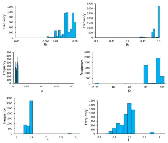
Figure 2.
Posterior distribution of soil water flow parameters: θr = residual soil water content, θs = saturated soil water content, Ks = is saturated hydraulic conductivity, l = tortuosity factor, α = empirical parameter, and n = empirical parameter. The x-axises of the plots are fixed to prior distribution (range) of the parameters.
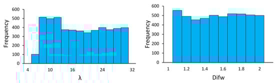
Figure 3.
Posterior distribution of solute transport parameters: Difw = diffusion coefficient and λ = dispersivity. The x-axises of the plots are fixed to prior distribution (range) of the parameters.
As it is illustrated, the posterior distributions of the parameters are different from their priors. The posterior distributions of water flow simulation as well as water stress reduction function parameters occupied small portion of their prior values. Thus, the parameters related to the advection process in the solute transport phenomenon have been estimated with high confidence (low uncertainty). These posterior distributions confirmed that the M-H algorithm was able to estimate the water flow parameters of the model with a low uncertainty level [58]. Nevertheless, the posterior distributions of dispersivity (λ) and diffusion coefficient (Dlw) did not considerably change from the corresponding priors (Figure 3). The posterior distributions of root water uptake reduction parameters (h50 and P1) for water stress have been remarkably changed after the M-H algorithm implementation for simulations of ECsw (Figure 4). However, the considerable uncertainty remained in the parameters of root water uptake reduction function for salinity stress (Figure 4) as their posterior distributions covered the prior ranges of the parameters. The unique relative sensitivity of the parameters was expected due to having atmospheric boundary conditions that constituted specific wetting and drying cycles. The relative sensitivity of the parameters to simulate soil salinity dynamics study was lower (higher CV) for solute transport and root water uptake reduction for salinity stress parameters compared to the parameters related to water flow simulation and root water uptake reduction function for water stresses (Table 6). The dispersivity (λ) was found as the least sensitive parameter compared to the others, and similar results were obtained by Skaggs et al., 2013 [59] for soil column experiments. The quantiles of the posterior distribution of the parameters are summarized in Table 7. The 95 CI output uncertainty of the model was obtained from the running model for 1000 parameter sets between the 2.5 and 97.5% quantiles.
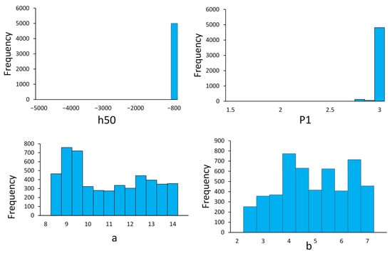
Figure 4.
Posterior distributions of root water uptake reduction parameters. The h50, P1, a, and b are the water pressure head for a 50% reduction in root water uptake, empirical parameter, threshold, and slope of root water uptake reduction function for salinity stress, respectively. The x-axises of the plots are fixed to prior distribution (range) of the parameters.
Table 7.
Quantiles of the posterior distribution of the model parameters.
3.2. Predictive Uncertainty
Figure 5 shows the 95 CI predictive band associated with the models’ parameters to simulate the dynamic of soil salinity at four different soil depths during and out of the growing season. The blue bands are 95 CI of the model outputs, and orange dots are observational points. The red bars in the figure sections are indicators of the end of irrigation events (close to the end of the growing season (a–d)), and the green bars are indicators beginning out of season rainfalls. The majority of the observational data are covered by the 95 CI band, which is an indicator of reaching parameter uncertainty to the model outputs [56]. Furthermore, covering most of the observational data in the 95 CI band shows that a significant portion of uncertainty in model outputs was due to existing uncertainty in the model parameters. However, at 70 cm (Figure 5d) soil depth, some of the observational points were out of the 95 CI band, which showed another source of uncertainty was influential at that specific soil depth. For evaluation of the predictive uncertainty, the r-factor and p-factor were calculated, and the results are presented in Table 5. The model output uncertainty is desirable if the 95 CI band covers 90% of observational data and the r-factor is less than one [55].
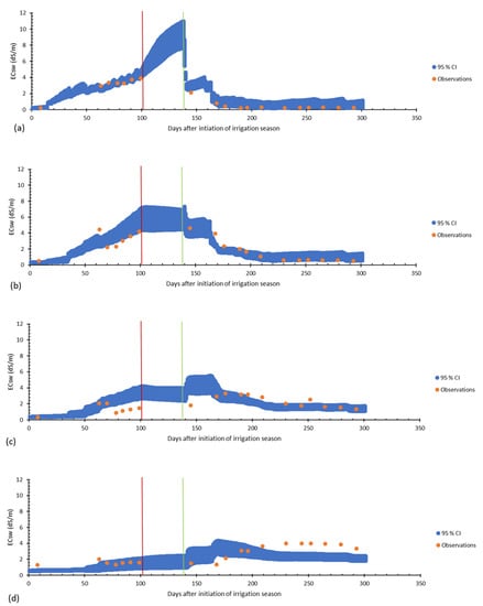
Figure 5.
Predictive uncertainty for simulating soil salinity dynamics during and out of growing season at (a) 10 (b) 30 (c) 50 and (d) 70 cm soil depth. Orange dots are measured values and blue bands are predictive uncertainty for parameters 95 CI.
Similar to predictive uncertainty graphs (Figure 5), the r- and p-factors results (Table 8) expressed a higher level of uncertainty for simulating soil salt dynamic at 50 and 70 cm soil depth. Furthermore, their corresponding the r-factors and p-factors were over 1 and below 100%, respectively, so the outputs of the model should be categorized as undesirable results.
Table 8.
Evaluation of the predictive uncertainty of the HYDRUS-1D model regarding soil salinity dynamic simulations.
As it is depicted in Figure 5, the 95 CI band is smaller during the irrigation season and rainy period out of the growing season. Hence, the predictive uncertainty of the HYDRUS-1D model was significantly higher during dry periods compared to wet periods in terms of simulating soil salinity dynamics.
3.3. Assessment of Simulated Soil Water Content and Salinity
The simulated time series of SWC are presented in Figure 6. The model’s SWC outputs were close to observational during the growing season and out of the growing season for two years of the study (2003 and 2004). Based on the statistical indices (Table 9), the overall performance of the HYDRUS-1D model was good regarding the SWC simulation.
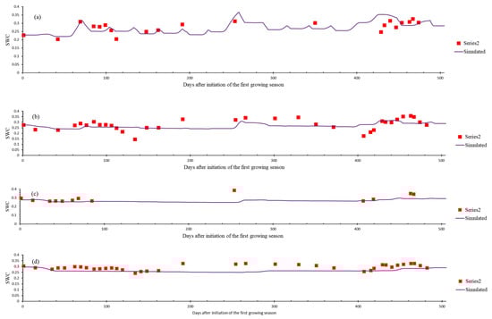
Figure 6.
Time series of the simulated soil water content during the growing season and out of the growing season with observational measurements at (a) 10, (b) 30, (c) 50, and (d) 70 cm soil depth.
Table 9.
Statistical indices to evaluate the performance of the -1D model regarding simulating soil water content.
The NRMSE values for SWC simulations were from 0.08 to 0.17 for four different soil depths that fall into good and excellent categories of the model accuracy, and the coefficient of agreement (d) values were from 0.5 to 0.78. The statistical indices and output graphs of the model (Figure 7) regarding the ECsw simulations validated the reliability of the calibrated model in reproducing the dynamics of soil salinity for two years. The d values were from 0.84 to 0.97 for the first three observational depths (10, 30, and 50 cm) and the corresponding NRMSE values were from 0.23 to 0.26, which were in the acceptable range. The highest deviations from the observational data were only found for simulated ECsw at 70 cm soil depth, which might not be desirable. The HYDRUS-1D model parameterized based on ECsw in saline water irrigation conditions was successful in reproducing the soil water movement, solute transport, and root water uptake process for two years during and out of the growing season.
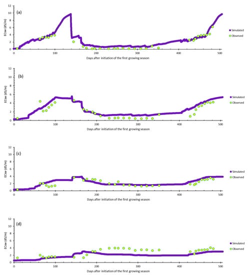
Figure 7.
Time series of the simulated ECsw during the growing season and out of the growing season with observational measurements for two years of study at (a) 10, (b) 30, (c) 50, and (d) 70 cm soil depth.
4. Discussion
Marginal water quality waters, such as saline water, have been known as alternative sources for agricultural systems to mitigate water scarcity. However, soil salinity is a potential threat in most cases for using these waters as irrigation water. The soil salinity can be controlled through irrigation management methods such as leaching application. The HYDRUS-1D is a well-known numerical model that could be used as a decision support tool to investigate irrigation water management strategies for using saline water as irrigation water. The proper calibration of this model is a common challenge that could be addressed by inverse solutions. The calibration of the models usually comes with some level of uncertainty that needs to be quantified and analyzed. The Markov Chain Monte Carlo (MCMC)-based algorithm, developed by pursuing the Bayesian theorem, has been known to be effective in exploring uncertainty aspects in the models’ calibrations. The algorithms that follow the Bayesian theorem integrate prior knowledge about the parameters of the models with available information about the specific study to calibrate the model and quantify the uncertainty by finding posterior distributions. In this study, the MCMC-based Metropolis-Hastings (M-H) algorithm was implemented for the HYDRUS-1D model to seek the posterior distributions of the model’s parameters to simulate the dynamics of soil salinity under saline irrigation conditions. The histograms and comparison of statistics of the prior and posterior distribution of the water flow simulation and root water uptake (RWU) reduction function for water stress parameters indicate that observational data included sufficient information to estimate these parameters [26]. The M-H algorithm was able to reasonably estimate residual soil water content (θr) at the field scale (CV = 0.04, SD = 0.003), which proved the algorithm’s effectiveness in estimating this parameter–which is complicated and time-consuming to be measured. The results indicated a higher level of uncertainty in diffusivity coefficient and dispersivity for solute transport simulations and threshold and slope of the RWU reduction function for salinity stress than the other parameters. A higher uncertainty level in solute transport parameters might be due to the scale of the study or some errors in the models’ inputs as an initial condition or boundary condition. Furthermore, the higher level of uncertainty in the threshold and slope parameters of the salinity stress reduction function is presumably due to the lack of sufficient knowledge in the literature for the vegetations of this study threshold to the soil salinity stress. Hence, the selection of our priors for these parameters might have encountered some errors that resulted in the insufficiency of the M-H algorithm in identifying them and reducing the uncertainty level. The posterior distributions of the parameters, which are concentrated in a specific part of the prior distribution, confirm the robustness of the Bayesian statistics concepts–specifically the M-H algorithm–in seeking the posterior distribution of the parameters and reducing the uncertainty. Similar highly concentrated results for seeking posterior distributions of the parameters of the crop models (DSSAT and large-scale crop model) have been reported by He et al., 2009 and Izumi et al., 2009 [58,60]. The results showed a higher level of uncertainty in model outputs during dry periods when no precipitation occurred. One of the hypotheses that could explain this matter is when the soil is exposed to drying (no irrigation or precipitation), the prevailing solute transport condition is more unsaturated than in the wet period, which could increase the complexity of the phenomena predicted by the model. The interactions of evapotranspiration and soil water, and solute fluxes under unsaturated conditions are more difficult to be reproduced by the model. The increase in the unsaturation level of the soil water would make it harder for the model to simulate the water flow and solute transport in the one-dimensional (1D) mode. The predictive uncertainty band covered most of the observational points in all of the observational depths except the 70 cm. This is an indicator of another source of uncertainty in addition to the uncertainty in the model parameters for this soil depth. Among multiple sources of uncertainty, it sounds reasonable to consider the measurement error accountable for these outsider points. However, there was a possibility that if another calibration was done for this soil layer, those points would be 95 CI. The validation of the HYDRUS-1D model, using continuous data for two years of the study, has proved the reliability of the calibration achieved by implementing the M-H algorithm. The model was able to successfully reproduce (Table 9) the ECsw and SWC during and out of the two growing seasons in 2003 and 2004 (Figure 6 and Figure 7). As indicated in the results, there are some detectable deviations in simulating ECsw at 70 cm soil depth. As mentioned in the results, the deviations were expected due to existing uncertainty in the model outputs. The output uncertainty was reflected in the model performance in terms of simulating soil salinity dynamics as the overall NRMSE value was more than 0.3, and R was equal to 0.52 at this soil depth. In this study, it has been proved that even if the target of calibration and uncertainty assessment of the HYDRUS-1D model is soil water salinity (ECsw), a very acceptable performance of the model can still be achieved. This is because the advection term in the advection-dispersion equation is usually the main driving force of the solute transport phenomenon in the soil porous media under saline irrigation conditions. This study’s findings authenticated the M-H algorithm’s solidity for exploring different aspects of the uncertainty in the HYDRUS-1D model to simulate salinity dynamics under saline water conditions.
The main challenges regarding the accomplishment of the current study to explore the uncertainty aspects of the HYDRUS-1D model for simulating the soil salinity were:
1. The lack of any reported values in the literature regarding the threshold of spontaneous crops to salinity stress.
2. The unavailability of additional data to validate the model performance for more than two years, specifically the recently obtained data that would contain the effects of climate change on the frequency of irrigation events and out-of-growing season precipitations.
To explore further aspects of the uncertainty of the HYDRUS-1D model, the following suggestion might be beneficial for further studies:
1. Testing additive approach for using the water and salinity stress reduction functions for mimicking root water uptake.
2. Investigating the Feddes model as a water stress reduction function [61].
3. Performing SWC and ECsw simulations for row crop cultivations such as corn and cotton.
4. Studying the uncertainty of the HYDRUS-1D model for simulating water and salinity dynamics under crop rotation schemes.
5. Furthermore, an investigation of the HYDRUS-1D uncertainty for reproducing SWC and ECsw under deficit irrigation with marginal quality waters would provide more information about uncertainty in the water and salinity stress reduction function parameters.
5. Conclusions
The uncertainty of the HYDRUS-1D model for simulating the dynamic of salts in the root zone at the field scale was assessed using the Metropolis-Hastings algorithm in the R-Studio environment. In this study, the uncertainty in the model’s soil water content, root water uptake and solute transport parameters, and outputs were explored based on measurement data of electrical conductivity of soil water (ECsw). The results of this study indicated a higher level of precision (low uncertainty) in parameters related to water movement simulations comparing with the solute transport parameters (specifically dispersivity and diffusivity). The results of the model’s output uncertainty (predictive uncertainty) showed a relatively lower level of uncertainty in ECsw during wet (under irrigation or rainfall) periods of the year compared with dry periods. The majority of output uncertainty in this study originated from parameter uncertainty. Moreover, it has been proved that even if the target of simulations for calibration and uncertainty purposes is ECsw, an excellent performance of the model can be achieved for simulating soil water content. Thus, the HYDRUS-1D outputs are reliable for investigating leaching requirement estimations scenarios to achieve proper irrigation scheduling for saline irrigation water conditions. However, to gain more insight into uncertainty aspects of the HYDRUS-1D model, it is highly recommended to pursue the uncertainty assessment of the model for simulating soil salt dynamic in the root zone of crops such as corn, wheat, or soybean under sprinkle or trickle irrigation systems.
Author Contributions
Conceptualization, F.M. and B.G.; methodology, F.M., A.M. and B.G.; supervision, A.M., J.A. and B.G.; software, F.M. and J.A.; investigation, F.M.; data curation, M.C.G.; resources, J.A. and H.A.; writing—original draft preparation, F.M.; writing—review and editing, F.M., A.M. and J.A. All authors have read and agreed to the published version of the manuscript.
Funding
The APC was funded by Kansas State University.
Institutional Review Board Statement
Not applicable.
Informed Consent Statement
Not applicable.
Data Availability Statement
The data could be available by requesting M.C.G.
Acknowledgments
The group of authors would like to thank Kansas State University for financially supporting the APC for this study. Special thanks to Gyuhyeong Goh, faculty member of the department of statistics at Kansas State University, for the professional comments on this study. In addition, the group of authors would express their gratitude to Maria C. Gonçalves, who is the author of this paper as well, for her remarkable contribution to this project.
Conflicts of Interest
The authors declare no conflict of interest.
References
- Singh, A. Conjunctive use of water resources for sustainable irrigated agriculture. J. Hydrol. 2014, 519, 1688–1697. [Google Scholar] [CrossRef]
- Chen, L.-J.; Feng, Q.; Li, F.-R.; Li, C.-S. Simulation of soil water and salt transfer under mulched furrow irrigation with saline water. Geoderma 2015, 241–242, 87–96. [Google Scholar] [CrossRef]
- Oster, J.D. Irrigation with poor quality water. Agric. Water Manag. 1994, 25, 271–297. [Google Scholar] [CrossRef]
- Huang, M.; Zhang, Z.; Zhai, Y.; Lu, P.; Zhu, C. Effect of Straw Biochar on Soil Properties and Wheat Production under Saline Water Irrigation. Agronomy 2019, 9, 457. [Google Scholar] [CrossRef]
- Yuan, C.; Feng, S.; Huo, Z.; Ji, Q. Effects of deficit irrigation with saline water on soil water-salt distribution and water use efficiency of maize for seed production in arid Northwest China. Agric. Water Manag. 2019, 212, 424–432. [Google Scholar] [CrossRef]
- Li, J.; Gao, Y.; Zhang, X.; Tian, P.; Li, J.; Tian, Y. Comprehensive comparison of different saline water irrigation strategies for tomato production: Soil properties, plant growth, fruit yield and fruit quality. Agric. Water Manag. 2019, 213, 521–533. [Google Scholar] [CrossRef]
- Hussain, R.A.; Ahmad, R.; Waraich, E.A.; Nawaz, F. Nutrient uptake, water relations, and yield performance lf different wheat cultivars (Triticum aestivum L.) under salinity stress. J. Plant Nutr. 2015, 38, 2139–2149. [Google Scholar] [CrossRef]
- Letey, J.; Hoffman, G.J.; Hopmans, J.W.; Grattan, S.R.; Suarez, D.; Corwin, D.L.; Oster, J.D.; Wu, L.; Amrhein, C. Evaluation of soil salinity leaching requirement guidelines. Agric. Water Manag. 2011, 98, 502–506. [Google Scholar] [CrossRef]
- Ayers, R.S.; Westcot, D.W. Water Quality for Agriculture; Food and Agriculture Organization of the United Nations: Rome, Italy, 1985; Volume 29. [Google Scholar]
- Corwin, D.L.; Grattan, S.R. Are Existing Irrigation Salinity Leaching Requirement Guidelines Overly Conservative or Obsolete? J. Irrig. Drain. Eng. 2018, 144, 02518001. [Google Scholar] [CrossRef]
- Corwin, D.L.; Rhoades, J.D.; Šimůnek, J. Leaching requirement for soil salinity control: Steady-state versus transient models. Agric. Water Manag. 2007, 90, 165–180. [Google Scholar] [CrossRef]
- Simunek, J.; Van Genuchten, M.T.; Sejna, M. The HYDRUS-1D software package for simulating the one-dimensional movement of water, heat, and multiple solutes in variably-saturated media. Univ. Calif.-Riverside Res. Rep. 2005, 3, 1–240. [Google Scholar]
- Zeng, W.; Xu, C.; Wu, J.; Huang, J. Soil salt leaching under different irrigation regimes: HYDRUS-1D modelling and analysis. J. Arid Land 2014, 6, 44–58. [Google Scholar] [CrossRef]
- Yang, T.; Šimůnek, J.; Mo, M.; Mccullough-Sanden, B.; Shahrokhnia, H.; Cherchian, S.; Wu, L. Assessing salinity leaching efficiency in three soils by the HYDRUS-1D and -2D simulations. Soil Tillage Res. 2019, 194, 104342. [Google Scholar] [CrossRef]
- Gonçalves, M.C.; Šimůnek, J.; Ramos, T.B.; Martins, J.C.; Neves, M.J.; Pires, F.P. Multicomponent solute transport in soil lysimeters irrigated with waters of different quality. Water Resour. Res. 2006, 42, W08401. [Google Scholar] [CrossRef]
- Noshadi, M.; Fahandej-Saadi, S.; Sepaskhah, A.R. Application of SALTMED and HYDRUS-1D models for simulations of soil water content and soil salinity in controlled groundwater depth. J. Arid Land 2020, 12, 447–461. [Google Scholar] [CrossRef]
- Phogat, V.; Yadav, A.K.; Malik, R.S.; Kumar, S.; Cox, J. Simulation of salt and water movement and estimation of water productivity of rice crop irrigated with saline water. Paddy Water Environ. 2010, 8, 333–346. [Google Scholar] [CrossRef]
- Slama, F.; Zemni, N.; Bouksila, F.; De Mascellis, R.; Bouhlila, R. Modelling the Impact on Root Water Uptake and Solute Return Flow of Different Drip Irrigation Regimes with Brackish Water. Water 2019, 11, 425. [Google Scholar] [CrossRef]
- Liu, B.; Wang, S.; Kong, X.; Liu, X.; Sun, H. Modeling and assessing feasibility of long-term brackish water irrigation in vertically homogeneous and heterogeneous cultivated lowland in the North China Plain. Agric. Water Manag. 2019, 211, 98–110. [Google Scholar] [CrossRef]
- Helalia, S.A.; Anderson, R.G.; Skaggs, T.H.; Šimůnek, J. Impact of Drought and Changing Water Sources on Water Use and Soil Salinity of Almond and Pistachio Orchards: 2. Modeling. Soil Syst. 2021, 5, 58. [Google Scholar] [CrossRef]
- Tan, X.; Shao, D.; Liu, H. Simulating soil water regime in lowland paddy fields under different water managements using HYDRUS-1D. Agric. Water Manag. 2014, 132, 69–78. [Google Scholar] [CrossRef]
- Karamouz, M.; Meidani, H.; Mahmoodzadeh, D. Inverse unsaturated-zone flow modeling for groundwater recharge estimation: A regional spatial nonstationary approach. Hydrogeol. J. 2022, 30, 1529–1549. [Google Scholar] [CrossRef]
- Wang, X.; Li, Y.; Wang, Y.; Liu, C. Performance of HYDRUS-1D for simulating water movement in water-repellent soils. Can. J. Soil Sci. 2018, 98, 407–420. [Google Scholar] [CrossRef]
- Stafford, M.J.; Holländer, H.M.; Dow, K. Estimating groundwater recharge in the assiniboine delta aquifer using HYDRUS-1D. Agric. Water Manag. 2022, 267, 107514. [Google Scholar] [CrossRef]
- Shafiei, M.; Ghahraman, B.; Saghafian, B.; Davary, K.; Pande, S.; Vazifedoust, M. Uncertainty assessment of the agro-hydrological SWAP model application at field scale: A case study in a dry region. Agric. Water Manag. 2014, 146, 324–334. [Google Scholar] [CrossRef]
- Zeng, W.; Lei, G.; Zha, Y.; Fang, Y.; Wu, J.; Huang, J. Sensitivity and uncertainty analysis of the HYDRUS-1D model for root water uptake in saline soils. Crop Pasture Sci. 2018, 69, 163–173. [Google Scholar] [CrossRef]
- Hartmann, A.; Šimůnek, J.; Aidoo, M.K.; Seidel, S.J.; Lazarovitch, N. Implementation and Application of a Root Growth Module in HYDRUS. Vadose Zone J. 2018, 17, 170040. [Google Scholar] [CrossRef]
- Li, J.; Zhao, R.; Li, Y.; Chen, L. Modeling the effects of parameter optimization on three bioretention tanks using the HYDRUS-1D model. J. Environ. Manag. 2018, 217, 38–46. [Google Scholar] [CrossRef]
- Ang, A.H.S.; Tang, W.H. Probability Concepts in Engineering: Emphasis on Applications to Civil and Environmental Engineering, 2e Instructor Site; John Wiley & Sons Incorporated: Hoboken, NJ, USA, 2007; ISBN 047172064X. [Google Scholar]
- Moreira, P.H.S.; van Genuchten, M.T.; Orlande, H.R.B.; Cotta, R.M. Bayesian estimation of the hydraulic and solute transport properties of a small-scale unsaturated soil column. J. Hydrol. Hydromech. 2016, 64, 30–44. [Google Scholar] [CrossRef]
- Blasone, R.-S.; Madsen, H.; Rosbjerg, D. Uncertainty assessment of integrated distributed hydrological models using GLUE with Markov chain Monte Carlo sampling. J. Hydrol. 2008, 353, 18–32. [Google Scholar] [CrossRef]
- Vrugt, J.A.; ter Braak, C.J.F.; Diks, C.G.H.; Schoups, G. Hydrologic data assimilation using particle Markov chain Monte Carlo simulation: Theory, concepts and applications. Adv. Water Resour. 2013, 51, 457–478. [Google Scholar] [CrossRef]
- Wang, H.; Wang, C.; Wang, Y.; Gao, X.; Yu, C. Bayesian forecasting and uncertainty quantifying of stream flows using Metropolis–Hastings Markov Chain Monte Carlo algorithm. J. Hydrol. 2017, 549, 476–483. [Google Scholar] [CrossRef]
- Zheng, Y.; Han, F. Markov Chain Monte Carlo (MCMC) uncertainty analysis for watershed water quality modeling and management. Stoch. Environ. Res. Risk Assess. 2016, 30, 293–308. [Google Scholar] [CrossRef]
- Raje, D.; Krishnan, R. Bayesian parameter uncertainty modeling in a macroscale hydrologic model and its impact on Indian river basin hydrology under climate change. Water Resour. Res. 2012, 48, W08522. [Google Scholar] [CrossRef]
- Nguyen, D.H.; Kim, S.-H.; Kwon, H.-H.; Bae, D.-H. Uncertainty Quantification of Water Level Predictions from Radar-based Areal Rainfall Using an Adaptive MCMC Algorithm. Water Resour. Manag. 2021, 35, 2197–2213. [Google Scholar] [CrossRef]
- Brooks, S.; Gelman, A.; Jones, G.; Meng, X.-L. Handbook of Markov Chain Monte Carlo; CRC Press: Boca Raton, FL, USA, 2011; ISBN 1420079425. [Google Scholar]
- Kunnath-Poovakka, A.; Ryu, D.; Eldho, T.I.; George, B. Parameter uncertainty of a hydrologic model calibrated with remotely sensed evapotranspiration and soil moisture. J. Hydrol. Eng. 2021, 26, 4020070. [Google Scholar] [CrossRef]
- Yang, X.; Li, Y.P.; Liu, Y.R.; Gao, P.P. A MCMC-based maximum entropy copula method for bivariate drought risk analysis of the Amu Darya River Basin. J. Hydrol. 2020, 590, 125502. [Google Scholar] [CrossRef]
- Xu, W.; Jiang, C.; Yan, L.; Li, L.; Liu, S. An adaptive metropolis-hastings optimization algorithm of Bayesian estimation in non-stationary flood frequency analysis. Water Resour. Manag. 2018, 32, 1343–1366. [Google Scholar] [CrossRef]
- Allen, R.G.; Pereira, L.S.; Raes, D.; Smith, M. Crop Evapotranspiration-Guidelines for Computing Crop Water Requirements-FAO Irrigation and Drainage Paper 56; FAO: Rome, Italy, 1998; Volume 300, p. D05109. [Google Scholar]
- Van Genuchten, M.T. A closed-form equation for predicting the hydraulic conductivity of unsaturated soils. Soil Sci. Soc. Am. J. 1980, 44, 892–898. [Google Scholar] [CrossRef]
- Skaggs, T.H.; van Genuchten, M.T.; Shouse, P.J.; Poss, J.A. Macroscopic approaches to root water uptake as a function of water and salinity stress. Agric. Water Manag. 2006, 86, 140–149. [Google Scholar] [CrossRef]
- Skaggs, T.H.; Shouse, P.J.; Poss, J.A. Irrigating forage crops with saline waters: 2. Modeling root uptake and drainage. Vadose Zone J. 2006, 5, 824–837. [Google Scholar] [CrossRef]
- Ritchie, J.T. Model for predicting evaporation from a row crop with incomplete cover. Water Resour. Res. 1972, 8, 1204–1213. [Google Scholar] [CrossRef]
- Wang, X.; Li, Y.; Chau, H.W.; Tang, D.; Chen, J.; Bayad, M. Reduced root water uptake of summer maize grown in water-repellent soils simulated by HYDRUS-1D. Soil Tillage Res. 2021, 209, 104925. [Google Scholar] [CrossRef]
- Zarate-Valdez, J.L.; Whiting, M.L.; Lampinen, B.D.; Metcalf, S.; Ustin, S.L.; Brown, P.H. Prediction of leaf area index in almonds by vegetation indexes. Comput. Electron. Agric. 2012, 85, 24–32. [Google Scholar] [CrossRef]
- Radcliffe, D.E.; Simunek, J. Soil Physics with HYDRUS: Modeling and Applications; CRC Press: Boca Raton, FL, USA, 2018; ISBN 1420073818. [Google Scholar]
- Genuchten, M.T.; Hoffman, G.J.; Hanks, R.J.; Meiri, A.; Shalhevet, J.; Kafkafi, U. Management aspect for crop production. In Soil Salinity under Irrigation; Springer: Berlin/Heidelberg, Germany, 1984; pp. 258–338. [Google Scholar] [CrossRef]
- Zhang, Y.; Arabi, M.; Paustian, K. Analysis of parameter uncertainty in model simulations of irrigated and rainfed agroecosystems. Environ. Model. Softw. 2020, 126, 104642. [Google Scholar] [CrossRef]
- Yang, J.; Reichert, P.; Abbaspour, K.C.; Xia, J.; Yang, H. Comparing uncertainty analysis techniques for a SWAT application to the Chaohe Basin in China. J. Hydrol. 2008, 358, 1–23. [Google Scholar] [CrossRef]
- Zhang, J.; Vrugt, J.A.; Shi, X.; Lin, G.; Wu, L.; Zeng, L. Improving Simulation Efficiency of MCMC for Inverse Modeling of Hydrologic Systems With a Kalman-Inspired Proposal Distribution. Water Resour. Res. 2020, 56, e2019WR025474. [Google Scholar] [CrossRef]
- Maas, E.V.; Hoffman, G.J. Crop salt tolerance—Current assessment. J. Irrig. Drain. Div. 1977, 103, 115–134. [Google Scholar] [CrossRef]
- Grieve, C.M.; Grattan, S.R.; Maas, E.V. Plant salt tolerance. ASCE Man. Rep. Eng. Pract. 2012, 71, 405–459. [Google Scholar]
- Abbaspour, K.C.; Johnson, C.A.; Van Genuchten, M.T. Estimating uncertain flow and transport parameters using a sequential uncertainty fitting procedure. Vadose Zone J. 2004, 3, 1340–1352. [Google Scholar] [CrossRef]
- Bouda, M.; Rousseau, A.N.; Konan, B.; Gagnon, P.; Gumiere, S.J. Bayesian uncertainty analysis of the distributed hydrological model HYDROTEL. J. Hydrol. Eng. 2012, 17, 1021–1032. [Google Scholar] [CrossRef]
- Steduto, P.; Hsiao, T.C.; Raes, D.; Fereres, E. AquaCrop—The FAO crop model to simulate yield response to water: I. Concepts and underlying principles. Agron. J. 2009, 101, 426–437. [Google Scholar] [CrossRef]
- He, J.; Dukes, M.D.; Jones, J.W.; Graham, W.D.; Judge, J. Applying GLUE for estimating CERES-Maize genetic and soil parameters for sweet corn production. Trans. ASABE 2009, 52, 1907–1921. [Google Scholar] [CrossRef]
- Skaggs, T.H.; Suarez, D.L.; Goldberg, S. Effects of soil hydraulic and transport parameter uncertainty on predictions of solute transport in large lysimeters. Vadose Zone J. 2013, 12, 1–12. [Google Scholar] [CrossRef]
- Iizumi, T.; Yokozawa, M.; Nishimori, M. Parameter estimation and uncertainty analysis of a large-scale crop model for paddy rice: Application of a Bayesian approach. Agric. For. Meteorol. 2009, 149, 333–348. [Google Scholar] [CrossRef]
- Homaee, M.; Feddes, R.; Dirksen, C. Simulation of root water uptake. Agric. Water Manag. 2002, 57, 127–144. [Google Scholar] [CrossRef]
Publisher’s Note: MDPI stays neutral with regard to jurisdictional claims in published maps and institutional affiliations. |
© 2022 by the authors. Licensee MDPI, Basel, Switzerland. This article is an open access article distributed under the terms and conditions of the Creative Commons Attribution (CC BY) license (https://creativecommons.org/licenses/by/4.0/).