A Simple Application for Computing Reference Evapotranspiration with Various Levels of Data Availability—ETo Tool

Abstract

Reference evapotranspiration (ETo) estimations may be used to improve the efficiency of irrigated agriculture. However, its computation can be complex and could require numerous weather data that are not always available for many locations. Different methods are available to estimate ETo when limited data are available, and the assessment of the most accurate one can be difficult and time consuming. There are some standalone softwares available for computing ETo but none of them allow for the comparison of different methods for the same or different datasets simultaneously. This paper aims to present an application for estimating ETo using several methods that require different levels of data availability, namely FAO-56 Penman–Monteith (PM), the Original and the three modified Hargreaves–Samani (HS and MHS1, MHS2 and MHS3), Trajkovic (TR) and the single temperature procedure (MaxTET). Also, it facilitates the comparison of the accuracy estimation of two selected methods. From an example case, for where the application was used to compute ETo for three different locations, results show that the application can easily and successfully estimate ETo using the proposed methods, allowing for statistical comparison of those estimations. HS proves to be the most accurate method for the studied locations; however, the accuracy of all methods tends to be lower for costal locations than for more continental sites. With this application, users can select the best ETo estimation methods for a specific location and use it for irrigation purposes.

1. Introduction

The computation of reference evapotranspiration (ETo), if accurate, may serve as a basis for decision-making in irrigated agriculture such as water management, irrigation system design and management, irrigation scheduling and crop modelling [1,2,3,4,5,6,7,8,9]. From all the methods available for estimating ETo, the FAO-56 application of the Penman–Monteith (PM) equation [4] is widely regarded as the most accurate. The method provides consistent ETo values in many regions and climates [10,11], and it can be used globally without the need for additional parameter estimations. It is well documented, has been implemented, has been extensively validated and, when compared with other methods, it has been accepted as an accurate ETo estimator [12,13,14,15,16,17,18]. The main constraint of the PM equation is the requirement of numerous weather data (air temperature, windspeed, relative humidity and solar radiation) that are not always available. The availability and reliability of weather datasets of radiation, relative humidity and wind speed may be limited in many regions of the globe, especially in developing countries. This limitation compelled different studies to develop simpler methods where only data on maximum and minimum air temperature and extra-terrestrial radiation are required, such as the Hargreaves and Samani [19], modified Hargreaves–Samani [20,21] and Trajkovic [22] methods. These methods were widely compared with PM by different authors [15,18,23,24,25,26,27,28]. However, without a computer application, this assessment is time consuming, even more so if one wants to compute ETo using different methods.

There are a few standalone softwares available for computing ETo, such as REF-ET [29], DailyET [30] and DSS ET [31], that allow for referencing ET estimations using several methods. However, besides all of them being Windows-based standalone software, none allow computing ETo for two datasets at the same time and easily comparing the obtained results.

The objective of this paper is to develop an application for (1) estimating reference evapotranspiration using several methods that require different levels of data availability and (2) to easily compare the estimation accuracy of two selected methods, namely comparing less weather data demanding methods. The theoretical basis of the application and its primary features are presented in this paper; an example of the use of the application, using observed and reanalysis data, is presented in the companion paper [32]. The application is available for download at https://bit.ly/ETo_Tool_app and a tutorial video can be found at https://youtu.be/B6snPkYu89I.

2. Conceptual Model and Accuracy Indicators

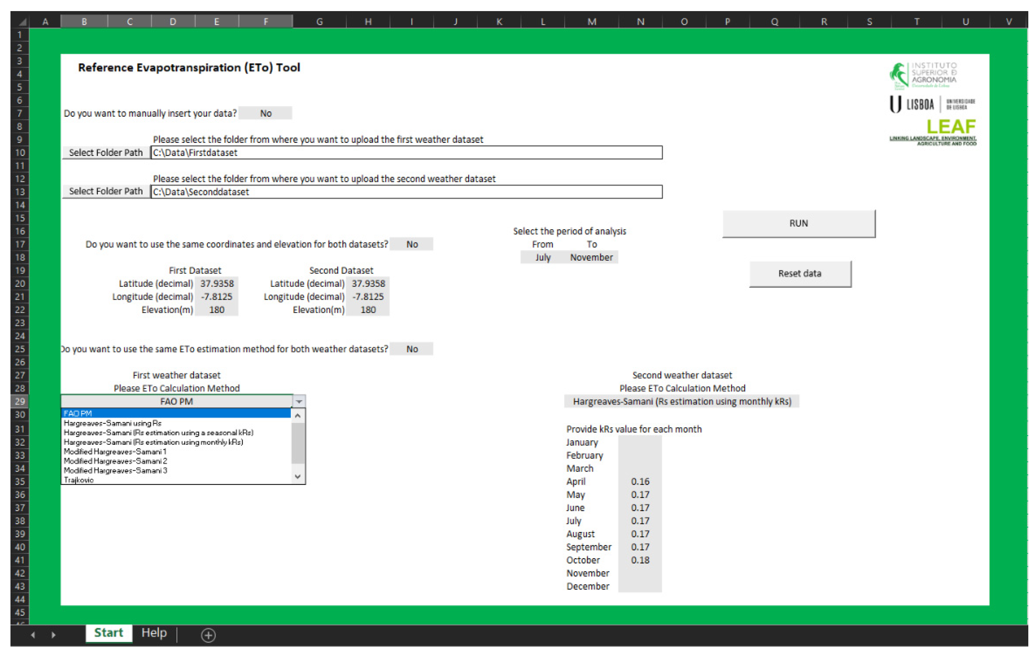
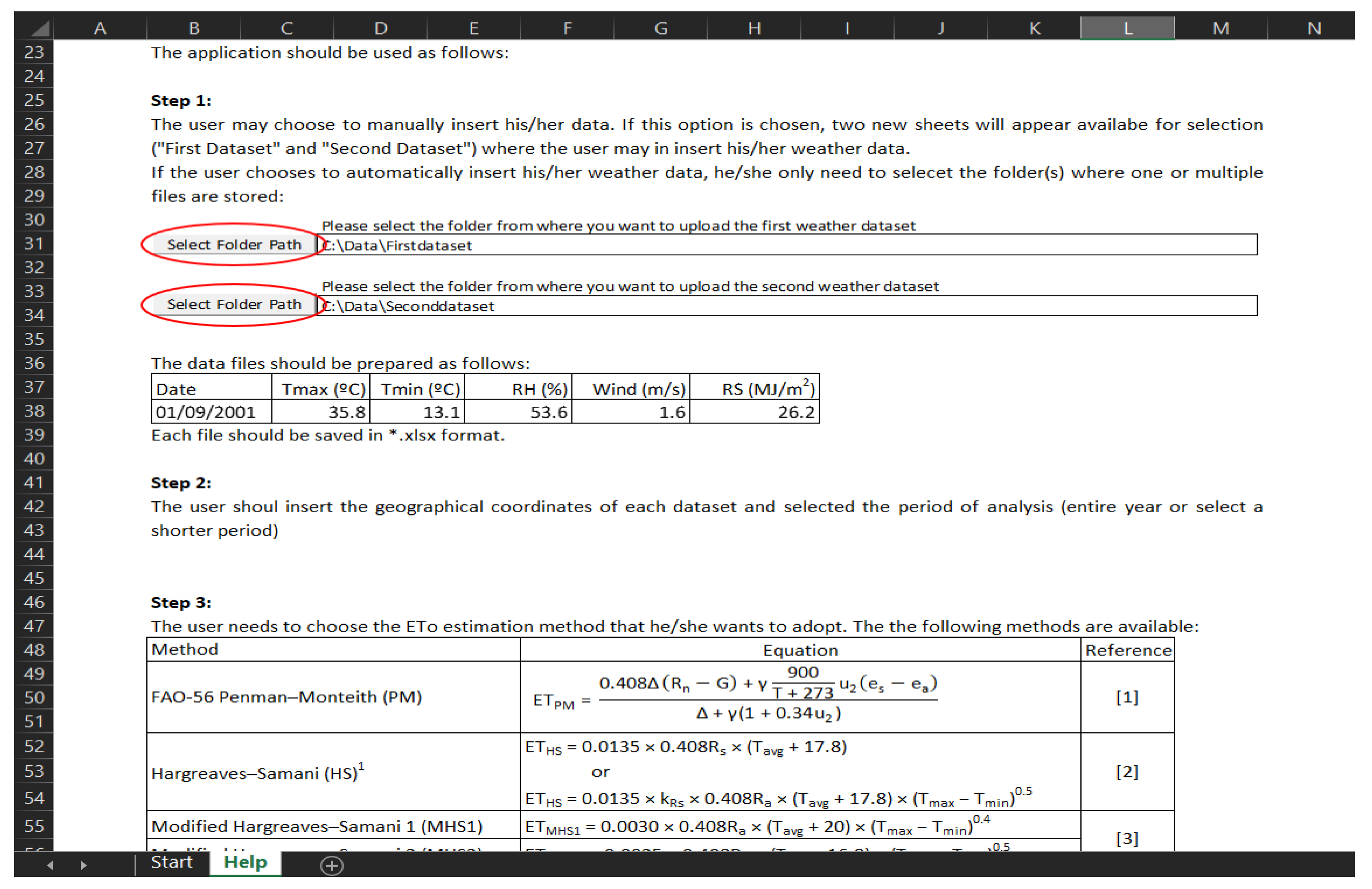
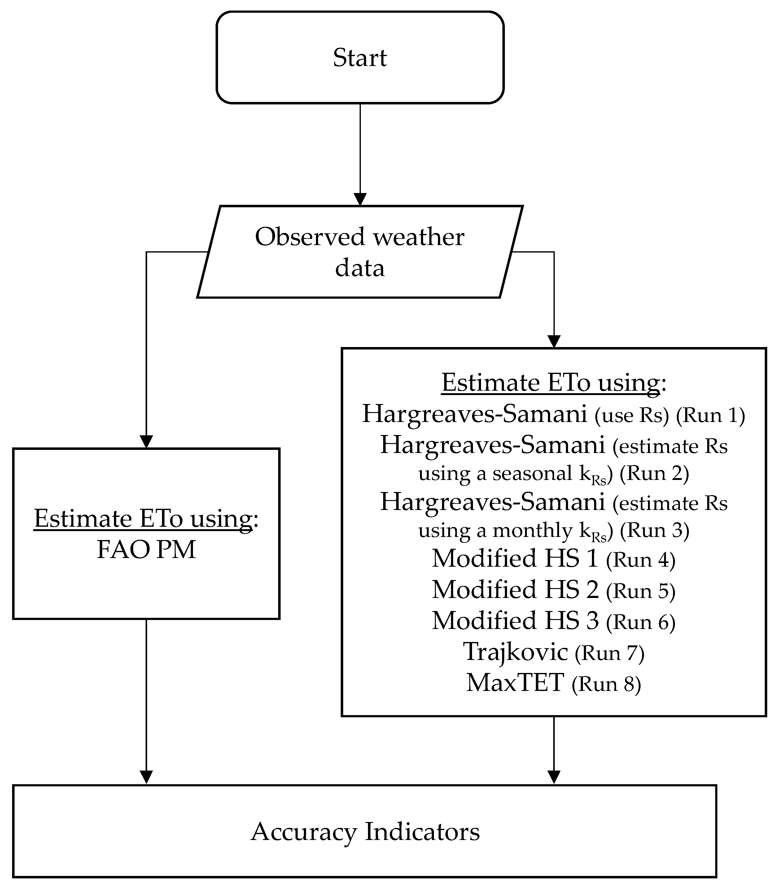
2.1. App Concept

The application has been programmed using the Visual Basic for Application (VBA) language and implemented as a Microsoft Excel© (Albuquerque, NM, USA) macro-enabled spreadsheet designated ETo Tool. This allows it to be run on any computer operating system, only requiring Microsoft Excel© and related Analysis ToolPak. ETo Tool computes reference evapotranspiration (ETo) at various time steps (daily to monthly) based on seven methods, which are described below. The estimation of ETo for two different locations at the same time can easily be done, enabling the statistical comparison of both resulting outputs. The user can choose to use the same location and ETo estimation method for both datasets, for the same location and two different methods or for two different locations and methods. The user may also choose to estimate ETo for the entire year or select a shorter period. We opted to give the user total flexibility for the task to be performed. The simplified flow chart of the ETo Tool is shown in Figure 1.

The application allows for estimating ETo using the following methods with varying degrees of data requirement:

(a) FAO-56 Penman–Monteith (PM)

The method, as proposed by Allen et al. [4], is expressed by:

$${\mathrm{ET}}_{\mathrm{PM}}=\frac{0.408\Delta \left({\mathrm{R}}_{\mathrm{n}}-\mathrm{G}\right)+\mathsf{\gamma }\frac{900}{\mathrm{T}+273}{\mathrm{u}}_2\left({\mathrm{e}}_{\mathrm{s}}-{\mathrm{e}}_{\mathrm{a}}\right)}{\Delta +\mathsf{\gamma }(1+0.34{\mathrm{u}}_2)}$$

(1)

where ET_PM is the grass reference evapotranspiration (mm day⁻¹); Rn is the net radiation (MJ m⁻² day⁻¹); G is the soil heat flux density (MJ m⁻² day⁻¹), considered as null for daily estimates; T is the daily mean air temperature (°C) at 2 m, based on the average of maximum and minimum temperatures; u₂ is the average wind speed at 2 m height (m s⁻¹); e_s is the saturation vapor pressure (kPa); e_a is the actual vapor pressure (kPa); (e_s − e_a) is the saturation vapor pressure deficit (Δe, kPa) at temperature T; Δ is the slope of the saturated vapor pressure curve (kPa °C⁻¹); γ is the psychrometric constant (0.0677 kPa °C⁻¹). The computation of all data required for calculating ETo follows the procedure proposed by Allen et al. (1998).

(b) Hargreaves–Samani (HS)

The Hargreaves–Samani method [19] estimates ETo using only the observed maximum and minimum temperatures and the estimation of the extraterrestrial radiation, and is expressed by:

ET_HS = 0.0135 × 0.408R_s × (T_avg + 17.8)

(2)

or

ET_HS = 0.0135 × k_Rs × 0.408R_a × (T_avg + 17.8) × (T_max − T_min)^0.5

(3)

where ET_HS is the grass reference evapotranspiration (mm day⁻¹); Rs is the solar radiation (MJ m⁻² day⁻¹); Ra is the extraterrestrial radiation (MJ m⁻² day⁻¹), 0.0135 is a factor for conversion from American to the International system of units; T_avg is the average air temperature (°C); T_max is the maximum air temperature (°C); T_min is the minimum air temperature (°C); k_Rs is the radiation adjustment coefficient (°C^−0.5). The empirical coefficient k_Rs was originally considered as 0.17 °C^−0.5 (Hargreaves and Samani, 1985). The use of a seasonal or monthly k_Rs is allowed.

(c) Modified Hargreaves–Samani 1 and 2 (MHS1 and MHS2)

Droogers and Allen [20] proposed two modifications of the original HS methods in order to improve ETo estimations. Those methods are expressed by:

ET_MHS1 = 0.0030 × 0.408R_a × (T_avg + 20) × (T_max − T_min)^0.4

(4)

ET _MHS2 = 0.0025 × 0.408R_a × (T_avg + 16.8) × (T_max − T_min)^0.5

(5)

(d) Modified Hargreaves–Samani 3 (MHS3)

Berti et al. [21] modified the original HS method as follows:

ET_MHS3 = 0.00193 × 0.408R_a × (T_avg + 17.8) × (T_max − T_min)^0.517

(6)

(e) Trajkovic (TR)

Trajkovic [22] proposed modified the original HS method as follows:

ET_Tr = 0.0023 × 0.408R_a × (T_avg + 17.8) × (T_max − T_min)^0.424

(7)

(f) Single temperature procedure (MaxTET)

The maximum temperature-based evapotranspiration (MaxTET) procedure, as proposed by Rodrigues and Braga [33], only uses maximum temperature to estimate ETo:

$${\mathrm{ET}}_{\mathrm{Tmax}}{=\mathrm{k}}_{\mathrm{Tmax}}{\times \mathrm{T}}_{\max }$$

(8)

where ET_Tmax is the reference crop evapotranspiration (mm day⁻¹), k_Tmax is the temperature adjustment coefficient (mm °C⁻¹) and T_max is the maximum air temperature (°C). The use of monthly k_Tmax that is locally calibrated is advisable.

Figure 2 shows a snapshot of the application interface. The application offers the possibility of manually inputting the weather data or to select the folder path where one or multiple dataset files are available may be uploaded into the spreadsheet. The data files must be in a standardized *.xlsx format; the first row must include the following information (one per column): date (dd/mm/year), maximum temperature (°C), minimum temperatures (°C), mean relative humidity (%), mean wind speed (m s⁻¹) and solar radiation (MJ m⁻² d⁻¹). The required inputs also include the geographical location of each station (latitude, longitude and elevation), the period of analysis and the method of ETo estimation to be used (as well as related coefficients, if required). For ETo estimation using temperature-based methods, maximum and minimum temperatures are mandatory. In this case, the remaining weather variables may be left blank. If the PM method is selected, mean relative humidity, mean wind speed and solar radiation are also required. In order to ease the use of the application, a help sheet (Figure 3) is avaiblable, with a step-by-step guide.

The results are presented in two different sheets: one with the computed results and scatter plot (Figure 4a); another with the accuracy indicators and statistical analysis. (Figure 4b)

2.2. Accuracy Indicators

The estimation accuracy of each variable was assessed through the metrics listed below, where FD_i and SD_i (i = 1, 2, …, n) represent pairs of values of ETo for the first and second datasets, respectively, $\overline{\mathrm{FD}}$ and $\mathrm{SD}$ are the respective mean values and n is the number of samples of each dataset:

• The coefficients of regression and determination, relating the first and second dataset, b and R², respectively, are defined as:

$$\mathrm{b}=\frac{{{\displaystyle \sum }}_{\mathrm{i}=1}^{\mathrm{n}}{\mathrm{FD}}_{\mathrm{i}}{\mathrm{SD}}_{\mathrm{i}}}{{{\displaystyle \sum }}_{\mathrm{i}=1}^{\mathrm{n}}{\mathrm{FD}}_{\mathrm{i}}{}^2}$$

(9)

$${\mathrm{R}}^2={\left\{\frac{{{\displaystyle \sum }}_{\mathrm{i}=1}^{\mathrm{n}}\left({\mathrm{FD}}_{\mathrm{i} }– \overline{\mathrm{FD}}\right)\left({\mathrm{SD}}_{\mathrm{i}} – \overline{\mathrm{SD}}\right)}{{\left[{{\displaystyle \sum }}_{\mathrm{i}=1}^{\mathrm{n}}{\left({\mathrm{FD}}_{\mathrm{i}} – \overline{\mathrm{FD}}\right)}^2\right]}^{0.5}{\left[{{\displaystyle \sum }}_{\mathrm{i}=1}^{\mathrm{n}}{\left({\mathrm{SD}}_{\mathrm{i}} – \overline{\mathrm{SD}}\right)}^2\right]}^{0.5}}\right\}}^2$$

(10)

Henseler et al. [34] defines that R² values of 0.25, 0.50 and 0.75 match weakly, moderately and significantly fit, respectively.

• The root mean square error, RMSE and its normalization, NRMSE, which characterizes the variance of the estimation error can be defined as:

$$\mathrm{RMSE}={\left[\frac{{{\displaystyle \sum }}_{i=1}^{\mathrm{n}}{\left(\mathrm{F}{\mathrm{D}}_{\mathrm{i} }– \mathrm{S}{\mathrm{D}}_{\mathrm{i}}\right)}^2}{\mathrm{n}}\right]}^{0.5}$$

(11)

$$\mathrm{NRMSE} =\frac{\mathrm{RMSE}}{ \overline{\mathrm{FD}}}\times 100\%$$

(12)

RMSE measures overall discrepancies between both datasets’ values and the smaller they are, the better accuracy. NRMSE is dimensionless, allowing comparison of its values for different variables, assuming a good fit with a normalization below 15%.

• The mean bias error, MBE, and its normalization, NMBE, that measures the systematic error between the second dataset and first dataset values can be defined as:

$$\mathrm{MBE}=\frac{{{\displaystyle \sum }}_{\mathrm{i}=1}^{\mathrm{n}}\left({\mathrm{SD}}_{\mathrm{i}}-{\mathrm{FD}}_{\mathrm{i}}\right)}{\mathrm{n}}$$

(13)

$$\mathrm{NMBE}=\frac{\mathrm{MBE}}{ \overline{\mathrm{FD}}}\times 100\%$$

(14)

The MBE and NMBE measure if the second dataset is over or under estimated with its positive or negative values, respectively. MBE intends to indicate the average interpolation bias [35].

• The Nash and Sutcliffe [36] modelling efficiency, EF, that is the ratio of the mean square error to the variance of the first dataset, subtracted from unity, can be defined as:

$$\mathrm{EF}=1.0 - \frac{{{\displaystyle \sum }}_{\mathrm{i}=1}^{\mathrm{n}}{\left({\mathrm{FD}}_{\mathrm{i}} {- \mathrm{SD}}_{\mathrm{i}}\right)}^2}{{{\displaystyle \sum }}_{\mathrm{i}=1}^{\mathrm{n}}{\left({\mathrm{FD}}_{\mathrm{i}} - \overline{\mathrm{FD}}\right)}^2}$$

(15)

As suggested by Legates and McCabe [37], if the square of the differences between the second and first datasets is as large as the variability in the observed data, then EF tends toward 0.0 and $\overline{\mathrm{FD}}$ is as good a predictor as the model, while negative values indicate that $\overline{\mathrm{FD}}$ is an even better predictor than the model. EF can vary between −∞ and 1.

The application also performs a one-way ANOVA, F-Test, t-Test and a descriptive statistics analysis, allowing for a more detailed comparison between both datasets (Figure 4b).

3. Example Case

In order to illustrate the use of ETo Tool, different mutilple runs, as presented in Figure 5, were performed for three different sites—Odemira, Beja and Elvas—to include coastal (Odemira), midland (Beja) and inland (Elvas) locations of Portugal (

Table 1. Location coordinates, elevation and distance to the sea.

Weather Station	Latitude (N)	Longitude (W)	Elevation (m)	Distance to the Sea (km)
Beja	38°02′15′′	07°53′06′′	206	79
Elvas	38°54′56′′	07°05′56′′	202	160
Odemira	37°30′06′′	08°45′12′′	92	4

). For each location, three different years were selected: humid, average and dry. Assuming a normal distribution for each dataset, the years when the ETo (during the irrigation months) is not exceeded with probabilities of 20, 50 and 80% were identified to represent low, average and high climatic demand, representing humid, average and dry years, respectively. The dataset for each location includes maximum and minimum temperature, solar radiation, relative humidity and wind speed.

Table 2. Accuracy indicators for the relationship between daily ETo estimated by the Penman–Monteith equation, by the temperature-based equations for Odemira and for three different years–humid, average and dry.

Year	ETo Estimation Method		Accuracy Indicators
			b	R2	NRMSE (%)	NMBE (%)	EF
Humid	HS	Using Rs	1.29	0.73	34.81	30.60	−0.98
		Using Seasonal kRs	1.12	0.62	22.82	12.60	0.15
		Using Monthly kRs	1.08	0.61	20.55	9.40	0.31
	MHS1		1.20	0.63	28.60	21.97	−0.33
	MHS2		1.18	0.62	28.01	19.31	−0.28
	MHS3		0.98	0.62	17.33	−1.25	0.51
	Tr		0.93	0.63	16.92	−6.43	0.53
	MaxTET		1.07	0.60	18.51	8.89	0.44
Average	HS	Using Seasonal kRs	1.18	0.84	24.00	18.72	0.31
		Using Monthly kRs	0.99	0.75	14.58	1.01	0.75
		Using Seasonal kRs	0.96	0.73	15.13	−1.99	0.73
	MHS1		1.08	0.75	17.80	10.43	0.62
	MHS2		1.05	0.75	16.27	6.94	0.68
	MHS3		0.87	0.75	18.73	−11.53	0.58
	Tr		0.83	0.75	21.78	−15.57	0.43
	MaxTET		0.95	0.67	17.27	−1.81	0.64
Dry	HS	Using Rs	1.17	0.80	22.95	17.07	0.29
		Using Seasonal kRs	1.01	0.75	14.58	1.52	0.71
		Using Monthly kRs	0.97	0.72	14.85	−1.58	0.70
	MHS1		1.09	0.78	17.00	10.38	0.61
	MHS2		1.07	0.74	17.02	7.57	0.61
	MHS3		0.88	0.74	17.78	−11.02	0.57
	Tr		0.84	0.77	20.29	−15.40	0.44
	MaxTET		0.96	0.73	14.44	−1.66	0.72

HS—Hargreaves-Samani method; MHS1—Modified Hargreaves-Samani 1 method; MHS2—Modified Hargreaves-Samani 2 method; MHS3—Modified Hargreaves-Samani 3 method; Tr—Trajkovic method; MaxTET—Single temperature procedure; Rs—solar radiation; k_Rs—radiation adjustment coefficient; b—coefficient of regression; R²—coefficient of determination; NRMSE—normalized root mean square error; NMBE—normalized mean bias error; EF—Nash and Sutcliffe modelling efficiency

,

Table 3. Accuracy indicators for the relationship between daily ETo estimated by the Penman–Monteith equation, by the temperature-based equations for Beja and for three different years–humid, average and dry.

Year	ETo Estimation Method		Accuracy Indicators
			b	R2	NRMSE (%)	NMBE (%)	EF
Humid	HS	Using Rs	1.01	0.99	8.13	1.58	0.99
		Using Seasonal kRs	1.05	0.88	14.16	6.15	0.84
		Using Monthly kRs	1.05	0.88	13.96	5.97	0.85
	MHS1		1.09	0.88	16.70	10.89	0.78
	MHS2		1.11	0.88	18.55	12.67	0.73
	MHS3		0.93	0.88	14.03	−6.39	0.85
	Tr		0.85	0.88	19.54	−13.95	0.70
	MaxTET		1.04	0.82	16.65	6.68	0.78
Average	HS	Using Rs	1.04	0.91	12.61	4.83	0.89
		Using Seasonal kRs	1.08	0.85	18.32	10.34	0.77
		Using Monthly kRs	1.08	0.85	18.32	10.22	0.77
	MHS1		1.11	0.85	21.17	14.94	0.70
	MHS2		1.14	0.85	23.32	17.20	0.63
	MHS3		0.95	0.85	15.36	−2.67	0.84
	Tr		0.87	0.85	19.50	−10.65	0.74
	MaxTET		1.08	0.82	19.96	11.51	0.73
Dry	HS	Using Rs	1.01	0.95	8.75	1.22	0.94
		Using Seasonal kRs	1.04	0.87	14.66	5.79	0.84
		Using Monthly kRs	1.04	0.88	14.34	5.55	0.85
	MHS1		1.08	0.87	17.11	10.48	0.78
	MHS2		1.11	0.87	18.83	12.37	0.74
	MHS3		0.92	0.87	14.85	−6.72	0.84
	Tr		0.84	0.87	20.32	−14.18	0.70
	MaxTET		1.05	0.83	16.98	7.83	0.79

and

Table 4. Accuracy indicators for the relationship between daily ETo estimated by the Penman–Monteith equation, by the temperature-based equations for Beja and for three different years–humid, average and dry.

Year	ETo Estimation Method		Accuracy Indicators
			b	R2	NRMSE (%)	NMBE (%)	EF
Humid	HS	Using Rs	1.03	0.94	9.93	4.50	0.93
		Using Seasonal kRs	1.07	0.83	18.39	9.35	0.76
		Using Monthly kRs	1.04	0.82	17.18	5.74	0.79
	MHS1		1.17	0.83	25.91	20.47	0.52
	MHS2		1.21	0.83	29.22	23.41	0.39
	MHS3		1.00	0.83	15.86	2.57	0.82
	Tr		0.91	0.83	17.19	−6.26	0.79
	MaxTET		1.04	0.80	18.43	7.29	0.76
Average	HS	Using Rs	0.97	0.92	10.82	−2.14	0.91
		Using Seasonal kRs	1.02	0.79	17.28	4.35	0.77
		Using Monthly kRs	0.98	0.80	16.22	0.79	0.80
	MHS1		1.11	0.79	22.59	15.18	0.61
	MHS2		1.15	0.79	24.89	17.70	0.53
	MHS3		0.95	0.79	16.90	−2.13	0.78
	Tr		0.87	0.79	20.36	−10.49	0.69
	MaxTET		0.99	0.79	17.07	2.07	0.78
Dry	HS	Using Rs	0.90	0.86	17.00	−8.98	0.81
		Using Seasonal kRs	0.95	0.75	19.39	−2.28	0.75
		Using Monthly kRs	0.92	0.77	19.25	−5.75	0.75
	MHS1		1.04	0.76	20.48	7.56	0.72
	MHS2		1.07	0.75	22.30	10.29	0.66
	MHS3		0.89	0.75	21.10	−8.33	0.70
	Tr		0.81	0.76	25.69	−16.28	0.55
	MaxTET		0.93	0.79	18.36	−4.09	0.77

summarize the accuracy indicators for the entire irrigation season for Odemira, Beja and Elvas, respectively, when comparing PM ETo with ETo estimated using all the methods available in the application, for three reference years–humid, average and dry. Results show that, when comparing ETo estimations, the accuracy of each method is dependent on the climatic demand and location. For a coastal location (Table 2)–Odemira—and a humid year, MH3 (lowest b and NMBE and highest EF) tends to lead to the best results, followed by TR and MaxTET. However, for ETo estimations in an average and dry year, the method that leads to the most accurate results is HS using a monthly k_Rs for both years. Differently, for Beja (Table 3)–a midland location—the HS (using Rs) method leads to the best results for all years. As for an inland location (Table 4)–Elvas—the accuracy results are similar to the ones for Beja, with the HS (using Rs) method outperforming the remaining methods. However, all methods for all years and locations present a moderate fit with R² higher than 0.5. Similar results were found by Rodrigues and Braga [28] for these locations.

Results also show that, for coastal locations, the accuracy of all methods tends to be lower than for more continental sites. Similar results were found by Martinez and Thepadia [38], as they found that HS performs worse for coastal regions of Florida than compared with other methods. Also, and since all methods are temperature-based, the effects of wind and relative humidity are not taken into account when estimating ETo. This can also explain the underperformance of HG using Rs for Odemira. Estévez et al. [39] obtained similar results, concluding that relative humidity data are relevant for accurate ETo calculations in coastal locations. These conclusions suggest that a sensitivity analysis of the impacts of wind, relative humidity and solar radiation on ETo estimations would be advisable.

Nonetheless, results show that the application allows for easily computation of ETo using different estimation methods and to statistically compare the results.

4. Conclusions

In this paper, an application for estimating reference evapotranspiration using seven different methods has been presented. It allows for the computation of ETo for two different datasets and to statistically compare the resulting estimations. This is simple and user-friendly Microsoft Excel© macro-enabled spreadsheet and is available for free download. This application facilitates (1) the calculation of ETo for two locations at the same time and (2) the calculation of ETo using the same or different estimation methods for both datasets, without any specific Operating System, and may be run on any platform. The FAO-56 PM equation is recommended as the standard for computing reference evapotranspiration. However, and since the use of this method may be limited due to the availability of data in areas where meteorological information is scarce, the application allows the user to choose from six different temperature-based methods with different levels of required data. Results indicate that the application can successfully estimate ETo using different methods, allowing statistically comparison of the estimations.

The application allowed comparing ET estimations from all methods for three locations (costal, midland and inland) of Portugal for three years of different climatic demand—humid, average and dry. Results show that the accuracy of each method is dependent on the climatic demand and location. For a coastal location, the Hargreaves–Samani method allows for accurate estimations of ETo when compared with the FAO-56 Penman–Monteith method. Results also show that, for coastal locations, the accuracy of all methods tend to be lower than for more continental sites. This may be due to the fact that, since all methods are temperature-based, the effects of wind and relative humidity are not taken into account when estimating ETo. These conclusions suggest that a sensitivity analysis of the impacts of wind, relative humidity and solar radiation on ETo estimations would be advisable.

It can be concluded that ETo Tool can be recommended for ETo estimations. Future work will be based on adding more methods, a feature that allows computing ETo with PM from reduced datasets and data visualization and a web version of this ETo estimation Tool for further simplification of use.

References

1. Doorenbos, J.; Pruitt, W.O. Guidelines for predicting crop-water requirements. In FAO Irrigation and Drainage Paper No. 24, 2nd ed.; FAO: Rome, Italy, 1977; p. 156. [Google Scholar]
2. Wright, J.L.; Jensen, M.E. Development and Evaluation of Evapotranspiration Models for Irrigation Scheduling. Trans. ASAE 1978, 21, 0088–0091. [Google Scholar] [CrossRef]
3. Jensen, M.E.; Burman, R.D.; Allen, R.G. Evapotranspiration and Irrigation Water Requirements; ASCE Manuals and Reports on Engineering Practices No. 70; American Society of Civil Engineers: New York, NY, USA, 1990; 360p. [Google Scholar]
4. Allen, R.G.; Pereira, L.S.; Raes, D.; Smith, M. Crop Evapotranspiration—Guidelines for Computing Crop Water Requirements. Irrigation and Drainage Paper 56; FAO: Rome, Italy, 1998; p. 300. [Google Scholar]
5. Allen, R.G.; Wright, J.L.; Pruitt, W.O.; Pereira, L.S.; Jensen, M.E. Water Requirements. In Design and Operation of Farm Irrigation Systems, 2nd ed.; Hoffman, G.J., Evans, R.G., Jensen, M.E., Martin, D.L., Elliot, R.L., Eds.; ASABE: Joseph, MI, USA, 2007; pp. 208–288. [Google Scholar]
6. Howell, T.A.; Evett, S.; Tolk, J.A.; Schneider, A.D. Evapotranspiration of Full-, Deficit-Irrigated, and Dryland Cotton on the Northern Texas High Plains. J. Irrig. Drain. Eng. 2004, 130, 277–285. [Google Scholar] [CrossRef]
7. Steduto, P.; Hsiao, T.C.; Raes, D.; Fereres, E. AquaCrop—The FAO crop model to simulate yield response to water: I. Concepts and underlying principles. Agron. J. 2009, 101, 426–437. [Google Scholar] [CrossRef] [Green Version]
8. Rodrigues, G.C.; Pereira, L.S. Assessing economic impacts of deficit irrigation as related to water productivity and water costs. Biosyst. Eng. 2009, 103, 536–551. [Google Scholar] [CrossRef] [Green Version]
9. Paredes, P.; Rodrigues, G.; Alves, I.; Pereira, L. Partitioning evapotranspiration, yield prediction and economic returns of maize under various irrigation management strategies. Agric. Water Manag. 2014, 135, 27–39. [Google Scholar] [CrossRef]
10. Allen, R.G.; Clemmens, A.J.; Burt, C.M.; Solomon, K.; O’Halloran, T. Prediction accuracy for project wide evapotranspiration using crop coefficients and reference evapotranspiration. J. Irrig. Drain. Eng. 2005, 131, 24–36. [Google Scholar] [CrossRef] [Green Version]
11. Allen, R.G.; Pruitt, W.O.; Wright, J.L.; Howell, T.A.; Ventura, F.; Snyder, R.; Itenfisu, D.; Steduto, P.; Berengena, J.; Yrisarry, J.B.; et al. A recommendation on standardized surface resistance for hourly calculation of reference ETo by the FAO56 Penman-Monteith method. Agric. Water Manag. 2006, 81, 1–22. [Google Scholar] [CrossRef]
12. Trajkovic, S. Temperature-Based Approaches for Estimating Reference Evapotranspiration. J. Irrig. Drain. Eng. 2005, 131, 316–323. [Google Scholar] [CrossRef]
13. Adeboye, O.B.; Osunbitan, J.A.; Adekalu, K.O.; Okunade, D.A. Evaluation of FAO-56 Penman-Monteith and temperature based models in estimating reference evapotranspiration using complete and limited data, application to Nigeria. Agric. Eng. Int. CIGR J. 2009, XI, 1–25. [Google Scholar]
14. Sentelhas, P.C.; Gillespie, T.J.; Santos, E.A. Evaluation of FAO Penman–Monteith and alternative methods for estimating reference evapotranspiration with miss-ing data in Southern Ontario, Canada. Agr. Water Manag. 2010, 97, 635–644. [Google Scholar] [CrossRef]
15. Mohawesh, O.E.; Talozi, S.A. Comparison of Hargreaves and FAO56 equations for estimating monthly evapotranspiration for semi-arid and arid environments. Arch. Agron. Soil Sci. 2012, 58, 321–334. [Google Scholar] [CrossRef]
16. Cobaner, M.; Citakoğlu, H.; Haktanir, T.; Kisi, O. Modifying Hargreaves–Samani equation with meteorological variables for estimation of reference evapotranspiration in Turkey. Hydrol. Res. 2016, 48, 480–497. [Google Scholar] [CrossRef]
17. Song, X.; Lu, F.; Xiao, W.; Zhu, K.; Zhou, Y.; Xie, Z. Performance of 12 reference evapotranspiration estimation methods compared with the Penman-Monteith method and the potential influences in northeast China. Meteorol. Appl. 2019, 26, 83–96. [Google Scholar] [CrossRef] [Green Version]
18. Paredes, P.; Fontes, J.C.; Azevedo, E.B.; Pereira, L.S. Daily reference crop evapotranspiration in the humid environments of Azores islands using reduced data sets: Accuracy of FAO-PM temperature and Hargreaves-Samani methods. Theor. Appl. Clim. 2018, 134, 595–611. [Google Scholar] [CrossRef]
19. Hargreaves, G.H.; Samani, Z.A. Reference Crop Evapotranspiration from Temperature. Appl. Eng. Agric. 1985, 1, 96–99. [Google Scholar] [CrossRef]
20. Droogers, P.; Allen, R.G. Estimating Reference Evapotranspiration Under Inaccurate Data Conditions. Irrig. Drain. Syst. 2002, 16, 33–45. [Google Scholar] [CrossRef]
21. Berti, A.; Tardivo, G.; Chiaudani, A.; Rech, F.; Borin, M. Assessing reference evapotranspiration by the Hargreaves method in north-eastern Italy. Agric. Water Manag. 2014, 140, 20–25. [Google Scholar] [CrossRef]
22. Trajkovic, S. Hargreaves versus Penman-Monteith under Humid Conditions. J. Irrig. Drain. Eng. 2007, 133, 38–42. [Google Scholar] [CrossRef]
23. Tabari, H.; Talaee, P.H. Local Calibration of the Hargreaves and Priestley-Taylor Equations for Estimating Reference Evapotranspiration in Arid and Cold Climates of Iran Based on the Penman-Monteith Model. J. Hydrol. Eng. 2011, 16, 837–845. [Google Scholar] [CrossRef]
24. Raziei, T.; Pereira, L.S. Estimation of ETo with Hargreaves–Samani and FAO-PM temperature methods for a wide range of climates in Iran. Agric. Water Manag. 2013, 121, 1–18. [Google Scholar] [CrossRef]
25. Valipour, M.; Eslamian, S. Analysis of potential evapotranspiration using 11 modified temperature-based models. Int. J. Hydrol. Sci. Technol. 2014, 4, 192. [Google Scholar] [CrossRef]
26. Valipour, M. Temperature analysis of reference evapotranspiration models. Meteorol. Appl. 2015, 22, 385–394. [Google Scholar] [CrossRef]
27. Akhavan, S.; Kanani, E.; Dehghanisanij, H. Assessment of different reference evapotranspiration models to estimate the actual evapotranspiration of corn (Zea mays L.) in a semiarid region (case study, Karaj, Iran). Theor. Appl. Clim. 2018, 137, 1403–1419. [Google Scholar] [CrossRef]
28. Rodrigues, G.; Braga, R. Estimation of Reference Evapotranspiration during the Irrigation Season Using Nine Temperature-Based Methods in a Hot-Summer Mediterranean Climate. Agriculture 2021, 11, 124. [Google Scholar] [CrossRef]
29. Allen, R.G. REF-ET: Reference Evapotranspiration Calculation Software for FAO and ASCE Standardized Equations; University of Idaho: Moscow, Russia, 2000. [Google Scholar]
30. Hess, T.M. Potential Evapotranspiration [DAILYET]; Silsoe College: Cranfield, UK, 1996. [Google Scholar]
31. George, B.A.; Reddy, B.R.S.; Raghuwanshi, N.S.; Wallender, W.W. Decision Support System for Estimating Reference Evapotranspiration. J. Irrig. Drain. Eng. 2002, 128, 1–10. [Google Scholar] [CrossRef]
32. Rodrigues, G.C.; Braga, R.P. Estimation of Daily Reference Evapotranspiration from NASA POWER Reanalysis Products in a Hot Summer Mediterranean Climate. Agronomy 2021, 11, 2077. [Google Scholar] [CrossRef]
33. Rodrigues, G.; Braga, R. A Simple Procedure to Estimate Reference Evapotranspiration during the Irrigation Season in a Hot-Summer Mediterranean Climate. Sustainability 2021, 13, 349. [Google Scholar] [CrossRef]
34. Henseler, J.; Ringle, C.; Sinkovics, R. The use of partial least squares path modeling in international marketing. Adv. Int. Mark. 2009, 20, 277–320. [Google Scholar]
35. Willmott, C.J.; Matsuura, K. On the use of dimensioned measures of error to evaluate the performance of spatial interpolators. Int. J. Geogr. Inf. Sci. 2006, 20, 89–102. [Google Scholar] [CrossRef]
36. Nash, J.E.; Sutcliffe, J.V. River flow forecasting through conceptual models part I—A discussion of principles. J. Hydrol. 1970, 10, 282–290. [Google Scholar] [CrossRef]
37. Legates, D.R.; McCabe, G.J., Jr. Evaluating the use of goodness-of-fit measures in hydrologic and hydroclimatic model validation. Water Resour. Res. 1999, 35, 233–241. [Google Scholar] [CrossRef]
38. Martinez, C.J.; Thepadia, M. Estimating Reference Evapotranspiration with Minimum Data in Florida. J. Irrig. Drain. Eng. 2010, 136, 494–501. [Google Scholar] [CrossRef]
39. Estévez, J.; Gavilán, P.; Berengena, J. Sensitivity analysis of a Penman-Monteith type equation to estimate reference evapotranspiration in southern Spain. Hydrol. Process. 2009, 23, 3342–3353. [Google Scholar] [CrossRef]
Figure 1. Simplified flow chart of ETo Tool application.
Agronomy 11 02203 g001
Figure 2. ETo Tool interface: input data and ETo estimation method selection.
Agronomy 11 02203 g002
Figure 3. ETo Tool interface: help.
Agronomy 11 02203 g003
Figure 4. ETo Tool interface: (a) computed results and scatter plot; (b) accuracy indicators and statically analysis.
Agronomy 11 02203 g004
Figure 5. Flow chart presenting the example application runs performed with ETo Tool.
Agronomy 11 02203 g005