Article

Delineation of Soil Texture Suitability Zones for Soybean Cultivation: A Case Study in Continental Croatia

Faculty of Agrobiotechnical Sciences Osijek, Josip Juraj Strossmayer University of Osijek, Vladimira Preloga 1, 31000 Osijek, Croatia
*
Author to whom correspondence should be addressed.
Agronomy 2020, 10(6), 823; https://doi.org/10.3390/agronomy10060823
Submission received: 10 May 2020 / Revised: 3 June 2020 / Accepted: 8 June 2020 / Published: 10 June 2020
(This article belongs to the Special Issue Cropping Systems Models for Sustainable and Intensive Management)

Abstract

:
Soil texture is a vital criterion in most cropland suitability analyses, so an accurate method for the delineation of soil texture suitability zones is necessary. In this study, an automated method was developed and evaluated for the delineation of these zones for soybean cultivation. A total of 255 soil samples were collected in the Continental biogeoregion of Croatia. Three methods for interpolation of clay, silt and sand soil content were evaluated using the split-sample method in five independent random repetitions. An automated algorithm for soil texture classification based on the United States Department of Agriculture (USDA) in 12 classes was performed using Python script. Suitability classes for soybean cultivation per soil texture class were determined according to previous agronomic and soybean land suitability studies. Ordinary kriging produced the highest accuracy of tested interpolation methods for clay, silt and sand. Highly suitable soil texture classes for soybean cultivation, loam and clay loam, were detected in the northern part of the study area, covering 5.73% of the study area. The analysis of classification results per interpolation method indicated a necessity of the evaluation of interpolation methods as their performance depended on the normality and stationarity of input samples.

Graphical Abstract

1. Introduction

Knowledge of naturally suitable locations for the cultivation of a particular crop type is a basis for effective natural resource management and sustainable agriculture [1]. The development of spatial models of cropland suitability analyses integrated with geographic information system (GIS) enabled decision-makers to develop a crop management system that increases yield and land productivity [2]. The selection of the relevant criteria is based on crop and site-specific requirements, typically compiled from previous studies or crop expert surveys in the study area. Land suitability analysis commonly integrates climate and soil criteria groups of specific land use [3]. Soil texture presents a vital criterion in the GIS-based soybean suitability analyses for the determination of locations with the highest potential yield increase [4,5]. Many soil physical and chemical properties are directly influenced by soil texture, affecting soil fertility and productivity [6,7]. Recent research proved the direct influence of soil texture on the important segments of the ecosystem, such as agricultural yield variability [8], soil microbial and structural recovery [9] and richness and diversity of soil bacterial communities [10]. Automation of classification algorithms allows more time-efficient and robust classification in comparison to the conventional manual approach [11]. Recently developed algorithms for soil classification cover a wide range of applications, most notably measurement of soil surface roughness [12], prediction of soil fertility [13] and estimation of degraded soils [14]. In addition, mapping of soil texture variability in both horizontal and vertical dimensions has been a subject of interest in previous studies [15,16]. The mapping of the GIS analysis results presents an effective tool in their distribution to the end-users, both for farmers on a large scale, as well as for land policy managers on a small (regional) scale. Such data representation does not require extensive knowledge of spatial data and therefore allows simple interpretation, especially when integrated into web GIS maps.
Interpolation overcomes the limited representation of the agricultural soil properties by discrete soil sampling. Instead, it incorporates these ground-truth data to predict soil properties and enable a continuous representation of the entire agricultural field [17]. Interpolation methods are generally divided into geostatistical and deterministic methods. According to [18], geostatistical interpolation methods model the uncertainty associated with a spatial estimation based on random function theory, while the deterministic methods use only the input sample values and mathematical functions for interpolation. Geostatistical methods also apply statistical functions to quantify the predictions’ uncertainty, in contrast to deterministic interpolation methods. The basic step in the implementation of the geostatistical interpolation methods is the variogram analysis for the fitting of the most suitable theoretical mathematical model to an empirical variogram [19]. The evaluation of the interpolation methods enables the selection of the optimal, most accurate interpolation method for a particular soil sample [20]. The interpolation accuracy of soil samples has a direct impact on the creation of land-use management plans and variable-rate applications in precision agriculture [21].
Soybean (Glycine max L.) is the main oilseed crop in the world, presenting a high-quality source of oil and protein [22,23]. The long-term projection by [24] predicts a 1.3% global annual increase of soybean yield, which does not meet the food demands in the world. The development of soybean suitability analyses is therefore necessary for the improvement of soybean yield, especially to land policy managers [25]. A study by [26] noted the importance of soybean introduction in the cropping system, allowing the effective exploitation of soil nutrients and the overall reduction of pesticides and herbicides in precision agriculture. Soil texture is proven to have a significant impact on soybean cultivation and yield [27,28]. Improvement of research regarding soybean yield enhancement and sustainability is essential to satisfy growing soybean global demands [29].
The purpose of this study was to delineate soil texture suitability zones for soybean cultivation using an automated soil texture classification algorithm in a GIS environment. The specific objectives of the study were to: (1) evaluate and select the most accurate method for the interpolation of clay, silt and sand from input samples, (2) automate the process of soil texture classification in a GIS environment and (3) provide a map of soil texture suitability zones for soybean cultivation at a regional scale.

2. Materials and Methods
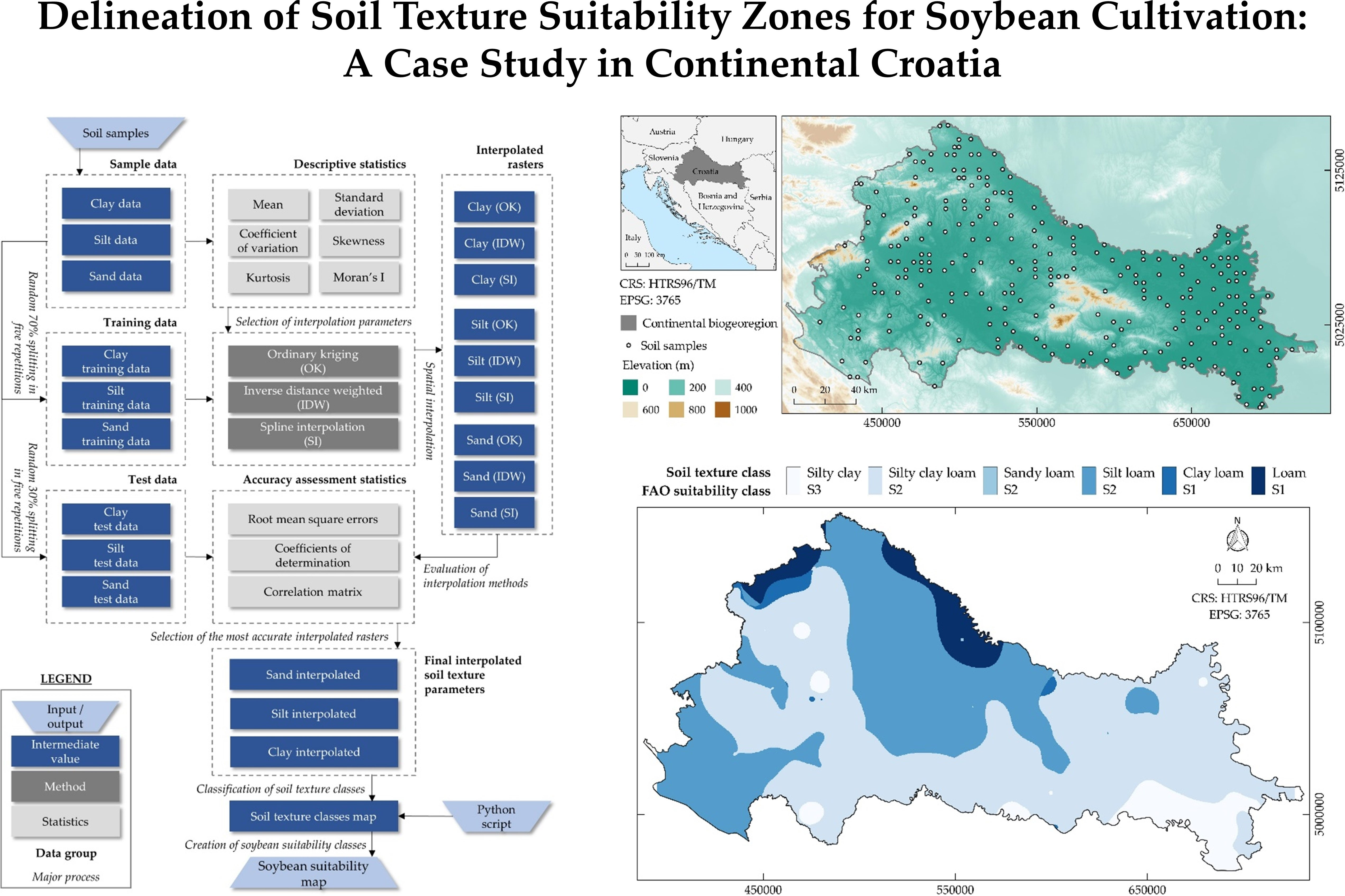
2.1. Study Area

The study area is the Continental biogeoregion of Croatia, covering 30,863 km2 and being one of the three national biogeoregions defined by the European Environment Agency [30] (Figure 1). The other two biogeoregions present in Croatia are alpine and Mediterranean biogeoregions. The study area is characteristically a moderately warm, rainy climate, as per Köppen’s classification. Soybean is gradually becoming one of the most produced crops in Croatia, with a 119% yield production increase between 2013 and 2016 as per Croatian Bureau of Statistics data. The terrain is dominantly lowland, at lower elevations. According to CORINE 2018 land cover data, agricultural areas represent the major land cover class with 54.0% of the study area. The second-largest land cover classes are forests and seminatural areas with 40.7% of the study area, followed by artificial surfaces (3.5%), water bodies (1.4%) and wetlands (0.5%).

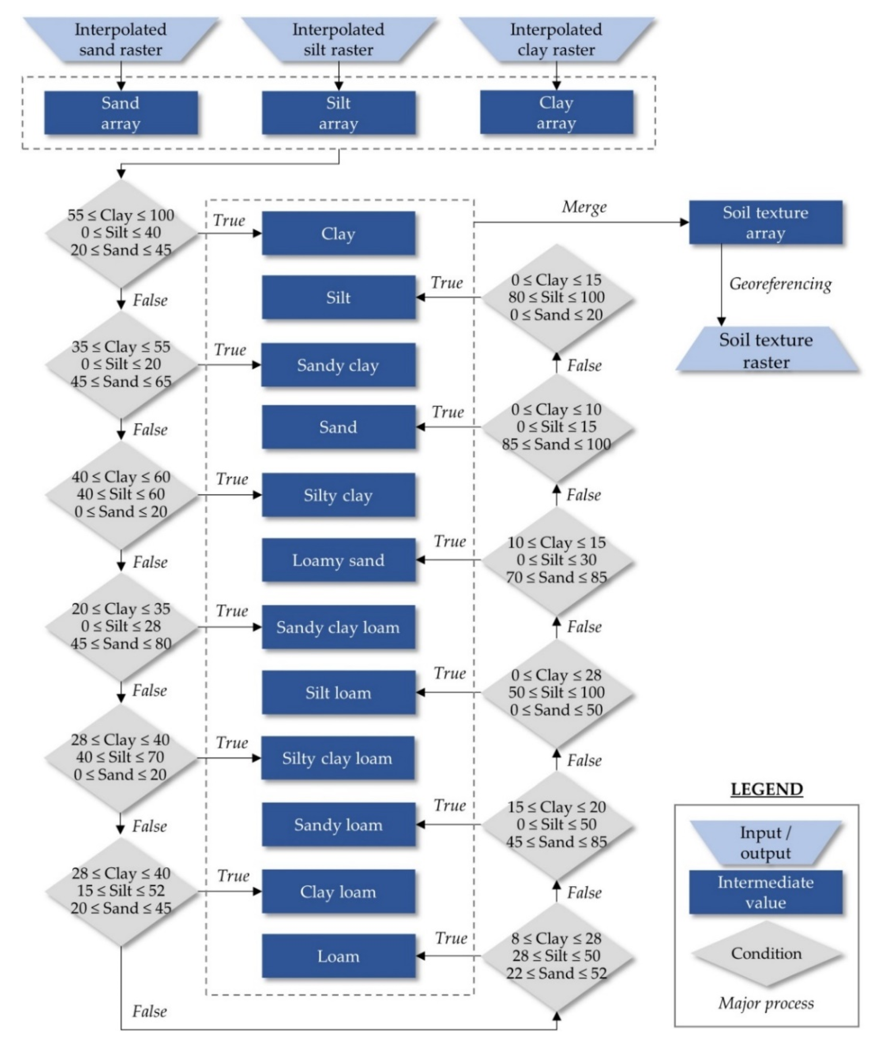
2.2. Automated Classification for Delineation of Soil Texture Suitability Zones for Soybean Cultivation in a GIS Environment

The selected interpolation methods for evaluation in this research were ordinary kriging (OK), inverse distance weighted (IDW) and spline interpolation (SI). These methods were recommended for the interpolation of soil properties by [31]. The workflow of this research is shown in Figure 2. All spatial calculations in this study were conducted using open-source GIS software: SAGA GIS v7.4.0 for the samples pre-processing and spatial interpolation and QGIS v3.8.3 for interpolation results and soil texture map visualization. Python v3.7.4 was used for scripting as a base for the automation of soil texture classification. The selected coordinate reference system (CRS) was the Croatian Terrestrial Reference System (HTRS96/TM). The spatial resolution of interpolated rasters was set to 250 m.
Input soil sample data was downloaded using the Croatian Agency for the Environment and Nature soil data WFS service. Soil samples were collected in the field according to ISO 11272:2017 and were pre-treated according to ISO 11464:2006 [32]. A total of 255 samples were collected in the study area during the year 2016. The soil texture content was determined by sieving and the sedimentation method prescribed in ISO 11277:2009. Soil fractions (<2 mm) were reclassified to three classes regarding particle size: clay (<0.002 mm), silt (0.002–0.063 mm) and sand (>0.063 mm). Each soil sample collected in the field represented a set of clay, silt and sand data on the same location. These values were filtered by attributes from input samples into a separate vector point layer in a GIS environment. The split-sample method was applied for the creation of training and test datasets, randomly splitting input samples to training data (70%) and test data (30%). From the total of 255 collected soil samples in the study area, 179 training samples and 76 test samples were randomly split from the original set individually for each repetition. The split-sample method was performed in five independent repetitions, resulting in five training and five corresponding test sample sets. Descriptive statistics consisting of mean, standard deviation (SD), coefficient of variation (CV), skewness (SK) and kurtosis (KT) were calculated to quantify normality and stationarity of the training sets. These properties are regarded as necessary for the determination of interpolation parameters for each method [33]. Normality designated the distribution of sample values, quantifying its deviation to normal distribution. Stationarity represented the number of local variations in the sample values, where low local variations indicate higher stationarity. Input data normality and stationarity are regarded as necessary indicators for the selection of optimal interpolation parameters [34].
OK is the most commonly used geostatistical interpolation method and is thoroughly described in [19,35]. It is also considered as the best linear unbiased spatial predictor [36]. OK incorporates a variogram as a tool for the modelling of spatial dependence between the input sample values and the mutual distance of samples [37]. The variogram was modelled based on (1):
γ ( h ) = 1 2 N x = 1 N [ Z ( x )     Z ( x + h ) ] 2 ,
where γ ( h )   is the semivariance, N is the number of sample pairs and Z ( x ) and Z ( x + h ) are the observation values at point x and at a point separated by h.
IDW is a deterministic interpolation method that predicts the values based on a weighted average of the input samples. The weights were assigned to each sample in an inversely proportional way to the distance from the predicted location [38]. The prediction principle of IDW is outlined in detail in [39].
SI is the deterministic interpolation method that performs the spatial interpolation by using the polynomial functions for describing the components of the interpolated area. Mutual fitting of those functions is performed, so that they join smoothly, consequentially resulting in the smooth representation of the interpolated area [17]. SI performs best in the case of gently varying surfaces, which is commonly associated with samples with high stationarity [31].
The three selected interpolation methods were applied to five randomly created training sets, resulting in 15 interpolation variations separately for clay, silt and sand soil content. The selection of interpolation parameters for all three interpolation methods was performed according to the evaluated normality and stationarity of the training sets. The existence and the range of the spatial variability of training samples and full samples were observed using Moran scatterplots, Moran’s I values and autocorrelograms [40]. All three tested interpolation methods were implemented in SAGA GIS software. OK was conducted with logarithmic transformation in the pre-processing due to lack of normal distribution of sample values for all soil parameters, as proposed by [41]. The starting parameters used for OK interpolation of training sets and final interpolation using full sample sets were a range of 170,000 m with 25 lags, with each lag covering a distance of 6800 m. Tested theoretical mathematical models for fitting to the empirical variogram were linear, square root, logarithmic, Gaussian and spherical. The selection of these models and corresponding ranges was performed based on the highest fitting coefficient of determination to the empirical variogram in ranges with existing spatial autocorrelation. The interpolation by the IDW method was performed by using the power parameter of 3 to prevent the emphasis of local variations in the interpolation results, due to moderate stationarity of training sets. SI was conducted by the thin plate spline process to ensure the smoothing of the interpolated surface to decrease the impact of higher local variabilities of the input samples [42]. The ranges of deterministic interpolation methods were selected based on observed spatial autocorrelation, amounting to maximum distances with continuous positive autocorrelation values.
Final clay, silt and sand soil content raster were interpolated with the full input sample data, using the most accurate interpolation method determined during accuracy assessment. Soil texture classification was performed in 12 classes according to the specifications of the United States Department of Agriculture (USDA) [43]. The classification process was automated using the algorithm realized in Python script (Figure 3, Appendix A). The automation in the GIS environment was developed to perform classification robustly and independently of the CRS, location extent, or spatial resolution of input rasters.

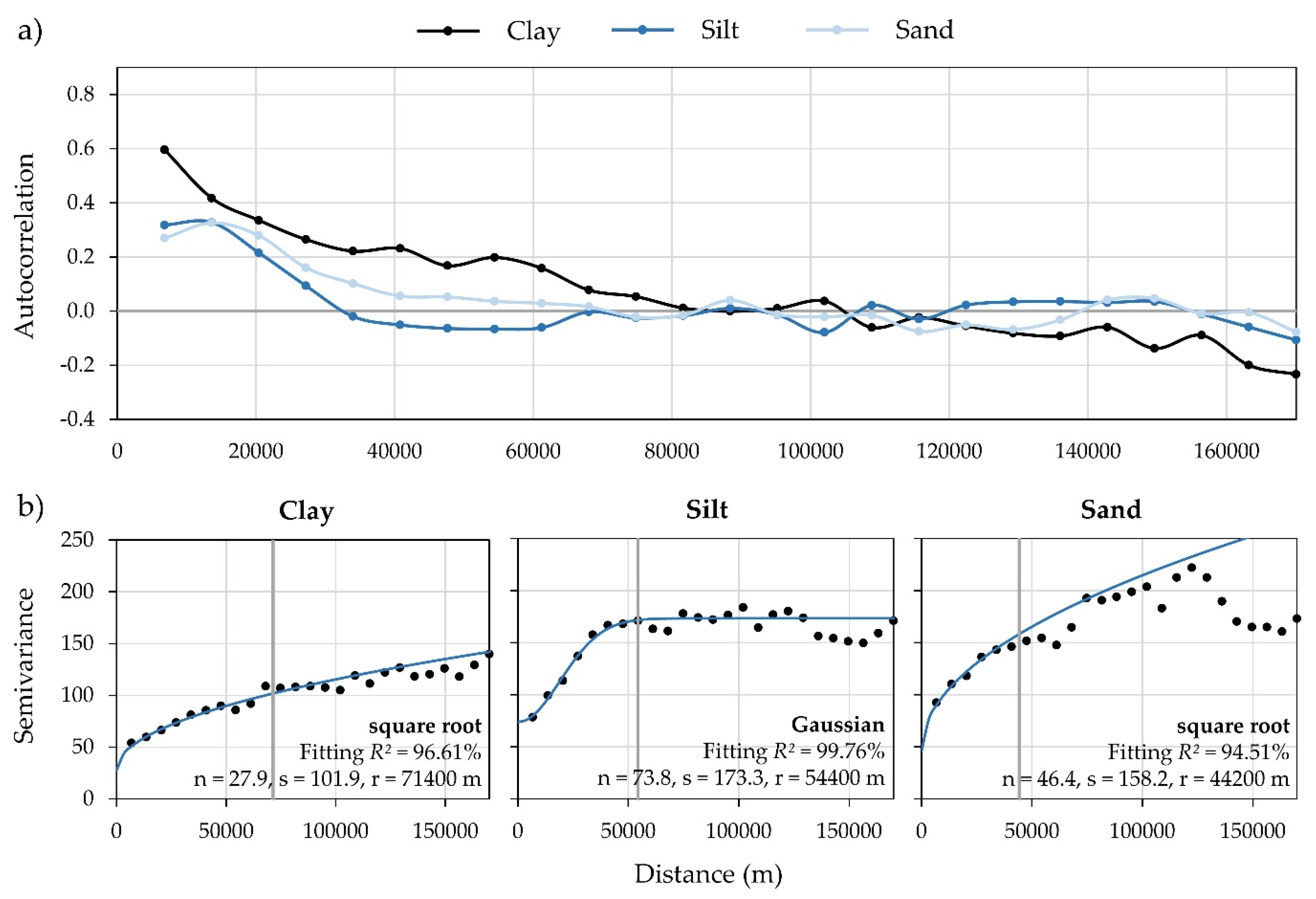
2.3. Accuracy Assessment of Interpolated Rasters

Accuracy assessment of the selected interpolation methods was conducted by the calculation of coefficients of determination (R2) and root-mean-square error (RMSE) for all interpolated rasters. These statistical values are considered as complementary for the evaluation of interpolation results for soil parameters [44]. The R2 quantified fitting of interpolated values to the regression line, while RMSE was used to assess variation in data based on absolute fit. The R2 values were calculated using a linear regression model. The higher R2 and lower RMSE indicate a better model fitting. Formulas for the calculation of R2 (2) and RMSE (3) were [45]:
R 2 = 1     1 n ( y i     y ^ i ) 2 1 n ( y i     y ¯ i ) 2 ,
R M S E = 1 n 1 n ( y i     y ^ i ) 2
where y i is the measured (sampled) value, y ^ i is the predicted value, y ¯ i is the average of the measured value y, and n is the number of observations.

2.4. Determination of Soybean Suitability Zones According to Soil Texture Classes

Loamy soil is the most suitable for the majority of crops, generally containing more organic soil matter and retaining moisture and nutrients better than other soil textures [46]. Levels of the suitability of 12 soil texture classes for soybean cultivation were evaluated based on previous soybean-specific agronomic and land suitability studies. Soybean-specific agronomic studies that evaluated the effects of soil texture for various applications in soybean cultivation are shown in Table 1. All evaluated studies noted a higher level of suitability for loamy textures compared to other classes present in the study area. Loamy soil textures with higher silt or clay content were regarded as more suitable compared to higher sand content, such as sandy loam or loamy sand. Recent studies based on GIS-based multicriteria land suitability for soybean cultivation containing soil texture as an influential criterion are shown in Table 2. The suitability of soil texture classes was natively represented according to Food and Agriculture Organization (FAO) specifications [47] or adjusted to this specification from original classes. FAO specifications for land suitability consist of five suitability zones: highly suitable (S1), moderately suitable (S2), marginally suitable (S3), marginally not suitable (N1) and permanently not suitable (N2). Similar to agronomic studies, loamy textures were considered as the most suitable, with clay loam and loam being regarded as highly suitable. Suitability levels generally decreased with the increase of clay, silt or sand soil contents. The final classification of soil texture suitability zones for soybean cultivation was performed according to FAO specifications and is presented in Figure 4.

3. Results

Descriptive statistics used for the estimation of training sample sets’ normality and stationarity are shown in Table 3. Silt soil content was observed as the dominant soil texture parameter in the study area, followed by clay. Clay and silt soil content data resulted in similar CV values through all five repetitions, representing low-variance data. Sand soil content produced CV values higher than 1.100 in all repetitions, indicating a high-variance data. SK remained consistent for all three soil parameters through repetitions. Clay and silt soil content resulted in right-tailed and left-tailed moderate skewness, respectively. Sand soil content consistently produces the highest SK values of all soil parameters, indicating a highly skewed data. KT resulted in the most variability of the calculated descriptive statistics for all soil parameters. However, values in all repetitions indicated a considerable platykurtic distribution for clay and silt soil contents and a considerable leptokurtic distribution for sand soil content. Sand soil content data values indicate a highly skewed distribution and moderate data stationarity.
The Moran scatterplot per training set is shown in Figure 5. Positive spatial autocorrelation was observed for all three soil parameters, with mean Moran’s I resulting in 0.396, 0.259 and 0.333 for clay, silt and sand, respectively. Interpolation ranges for IDW and SI per training sample set are presented in Appendix B. Mean distances until negative autocorrelation values were 81,600 m for clay, 29,920 m for silt and 54,400 m for sand. Variograms and interpolation parameters using OK for five training sample sets are presented in Appendix B. Square root and Gaussian theoretical mathematical models allowed the best fitting on most occasions, being applied 6 times each.
OK resulted in the highest mean RMSE and R2 values for all soil parameters and was determined as the most accurate interpolation method in this study (Table 4). It was followed by IDW as the second most accurate method according to both statistical values, while SI was the least accurate interpolation method. The interpolation results within the same soil parameter and interpolation methods generally produced high variability in accuracy values. Most notably, the difference between maximum and minimum values for RMSE was 2.26 for clay interpolation using SI, while R2 was 0.353 for the interpolation of clay using IDW. All three interpolation methods produced the highest accuracy for the interpolation of sand, followed by clay and silt soil contents.
Autocorrelogram and OK interpolation parameters of full sample sets are shown in Figure 6. Deterministic interpolation methods were performed with maximum ranges of 81,600 m for clay, 27,200 m for silt and 68,000 m for sand, matching maximum distances with positive autocorrelation. The specific local variabilities of the interpolation results were analysed according to Figure 7. OK produced interpolation results with low extreme values, compared to IDW and SI results. Consequentially, local variability in all soil fractions was minimized in interpolation results. Generalization of the local variabilities for OK is particularly noticeable in the south-west part of the study area for sand soil content interpolation. IDW results displayed the effects of all local variabilities to some degree but restricted their impact on interpolated results on local surroundings of the training samples. SI was the most balanced interpolation method considering the effects of local variabilities. The effects of local variations were retained in the interpolation results, having higher impacts on the surroundings of the training samples than IDW.
Histograms of interpolation results enabled quantification of the effect of local variabilities in the interpolation results (Figure 8). IDW resulted in the narrowest value interval of the tested interpolation method while having the top frequency value for every soil parameter. In contrast, SI produced the most variability regarding the interpolation values interval. Standard deviations of sand interpolation resulted in the greatest variability, with 7.91 for OK, 9.90 for IDW and 12.80 for SI.
The correlation matrix of tested interpolation methods for the respective soil fractions is displayed in Table 5. The maximum correlation was achieved for silt interpolation between IDW and SI. The lowest correlation was observed between OK and SI for both clay and sand interpolation. The visualization of classified soil texture in soil texture triangles is performed in Figure 9. OK produced the lowest dispersion of soil texture classes, dominantly covering silty clay loam and silt loam. IDW and SI covered a slightly wider range of soil texture classes. This observation particularly refers to loam, which is present in ground truth data (255 soil samples), but under-classified by OK. Both deterministic methods showed a notable presence of results in silty clay and clay loam classes, however, these classes had a low presence in ground truth data.
The interpolation of final clay, silt and sand soil fractions was performed by OK, as the most accurate interpolation method, with all 255 input samples. The results of the soil texture classification using Python script are displayed by coverage per soil texture class (Table 6). Loam and clay loam, as the two most suitable soil texture zones for soybean cultivation, were detected in the northern part of the study area, mostly covering the border area near the river Drava. Silt loam and silty clay loam, the two moderately suitable zones, covered 88.22% of the study area. Silty clay, as the only marginally suitable zone, was mostly present in the south-east on the study area. The soybean suitability thematic map according to soil texture classes is shown in Figure 10.

4. Discussion

The first objective of the study regarding the selection of the most accurate interpolation method was fulfilled by accuracy assessment based on five independent random split samples. Clay and silt possessed values moderately deviated from a normal distribution and moderate data stationarity, while sand possessed highly skewed values. Previous studies [60,61,62,63] suggested that these cases are common in analyses of soil properties, so the transformation of skewed data was determined as a necessary procedure in the algorithm. The application of logarithmic transformation in the pre-processing to OK minimized the effect of skewed distribution, as suggested by [64]. The descriptive statistics of clay, silt and sand in this study suggest that the thresholds for performing logarithmic transformation could be CV > 0.500 as the first condition, and the second condition that SK and KT deviate 0.500 or more from values of the normal distribution sample of zero and three, respectively. However, it is necessary to test this assumption on the different soil samples to evaluate its reliability. Similar studies imply the applicability of statistical tests like the Shapiro–Wilk [65] or Kolmogorov–Smirnov test [66] for the evaluation of data normality and could present an upgrade to the soil classification algorithm in future research. Sparse sampling density of one sample per 118 km2 used in this study is expected to have an impact on overall interpolation accuracy results. Denser soil sampling is expected to result in the lower CV of soil parameter values [67] and more accurate interpolation results [68,69]. However, the mapping of soil properties on a large scale was successfully performed using low-density samples, using one sample per 199 km2 in [70] and even one sample per 443 km2 in [71]. Due to the structure of the workflow and automatic soil texture classification algorithm in a GIS environment, a similar performance is expected by adding more samples in the existing area or using the same number of samples on a smaller area. Slightly more time-expensive computation in these cases is the only notable difference expected, as more input data should be processed.
The highest fitting R2 values for OK were achieved on shorter distances with full sample sets (71,400 m, 54,400 m and 44,200 m, compared to 84,320 m, 69,360 m and 119,680 m) in contrast to mean values of five training sample sets, which correspond better to observed spatial autocorrelation. OK was determined as the most accurate interpolation method for all three soil fractions, with R2 ranging from 0.592 to 0.784 and RMSE from 1.81 to 3.10. IDW was the second most accurate method, resulting in the most uniform accuracies through the interpolation repetitions. Moderate interpolation accuracies imply the necessity for denser soil samples in soil texture classification on a national level [72]. Sampling using regular grids proved in most cases to be the optimal suitable field sampling method [73]. The evaluation of interpolation methods displayed the importance of testing multiple methods. Mean R2 differences between OK as the most accurate and SI as the least accurate methods were 0.267 for clay, 0.189 for silt and 0.255 for sand. Mean RMSE differences showed the same trend, amounting to 1.60 for clay, 0.84 for silt and 1.28 for sand. The correlation matrix supported the previous statement, as the lowest correlation was observed between OK and deterministic interpolation methods, especially SI. OK also produced the most accurate interpolation results in a similar study, compared to deterministic interpolation methods [31]. However, a study by [34] proved that in the case of low sample data normality and stationarity, deterministic methods like IDW produce more accurate results than OK. The accuracy assessment in five independent repetitions was proven to be effective, as it allowed testing of interpolation performances in variable conditions. The interpolation results of IDW and SI were suitable for maintaining the effects of local soil variabilities, however the same can be achieved by the modifications of OK parameters if necessary [74].
The fulfilment of the second objective of the study regarding the automation of soil texture classification enabled the operator to avoid manual reclassification of classes. Automation of the classification process naturally resulted in shorter processing time than by manual tools execution [75]. Lower human interference in the data processing also provided a uniform classification result regardless of the input data, as well as its universal applicability. Recent advances in machine learning algorithms development allowed their implementation and automation in soil texture mapping, also presenting a new possibility in future research [76]. The current limitation of this study is the full automation of the interpolation and classification algorithm, which could be performed by R or Python programming languages.
The applied soil texture classification algorithm allowed the delineation of soil texture suitability zones, which is often used as a criterion in various GIS-based multicriteria analysis studies. Soil texture was an impactful criterion in many natural resource management studies: grassland conservation [77], irrigation management [78], soil salinity analyses [79] and drought risk assessment [80]. Future directions of suitability analyses using soil texture zones are planned for vegetable suitability multicriteria analyses, which are highly beneficial in sustainable planning [81].

5. Conclusions

The automation of soil texture classification enabled time-efficient delineation of suitability zones for soybean cultivation. Clay, silt and sand soil contents were evaluated using a random split-sample method in five repetitions, which ensured the objective determination of training data normality and stationarity. The descriptive statistics of evaluated training data indicated moderate data normality and stationarity for clay and silt, while sand soil content resulted in highly skewed distribution and moderate stationarity. The application of logarithmic transformation as a pre-processing to OK reduced the effect of non-normal distribution, particularly for the sand soil fraction. Tested deterministic methods, IDW and SI, produced lower interpolation accuracy values than OK, but were considered as viable methods in the case of low data normality and stationarity. The authors recommend the evaluation of interpolation methods for suitability calculations, as their performance is variable and depends on the properties of input samples. It was also observed that these methods were effective in retaining the local variation data in the interpolation result. Loam and clay loam were determined as the most suitable soil texture zones for soybean cultivation, covering the northern part of the study area near the river Drava. Classified soil texture classes with the highest presence in the study area were moderately suitable silty clay loam (53.26%) and silt loam (34.96%). According to the proposed methods, the study area is dominantly moderately suitable for soybean cultivation, based on the soil texture data. The integration of Sentinel-2 multispectral satellite images and GIS-based multicriteria analysis with current results presents the foundation of future research.

Author Contributions

Conceptualization, D.R.; methodology, D.R.; software, D.R.; validation, M.J., V.Z. and I.P.; formal analysis, D.R.; investigation, D.R.; resources, M.J., V.Z. and I.P.; data curation, D.R.; writing—original draft preparation, D.R.; writing—review and editing, D.R., M.J., V.Z. and I.P.; visualization, D.R.; supervision, M.J. and I.P.; funding acquisition, M.J. and I.P. All authors have read and agreed to the published version of the manuscript.

Funding

This research received no external funding.

Acknowledgments

This work was supported by the Faculty of Agrobiotechnical Sciences Osijek as a part of the scientific project “AgroGIT—Technical and Technological Crop Production Systems, GIS and Environment Protection”.

Conflicts of Interest

The authors declare no conflict of interest.

Appendix A. Automatic Soil Texture Classification Algorithm Scripted in Python

#import of the required libraries
import gdal
import numpy
from osgeo import osr
import os
#import of interpolated clay, silt and sand soil content rasters (marked in italic)
clay_all = gdal.Open(‘clay.tif’)
clay_band = clay_all.GetRasterBand(1)
clay = clay_band.ReadAsArray()
silt_all = gdal.Open(‘silt.tif’)
silt_band = silt_all.GetRasterBand(1)
silt = silt_band.ReadAsArray()
sand_all = gdal.Open(‘sand.tif’)
sand_band = sand_all.GetRasterBand(1)
sand = sand_band.ReadAsArray()
#assignment of new soil texture raster
soil_texture = clay
[cols,rows] = soil_texture.shape
#automatic classification function for soil texture
def classification (clay,silt,sand,x,y):
    soil_texture_class = 0
    if 55 <= clay[x][y] <= 100 and 0 <= silt[x][y] <= 40 and 20 <= sand[x][y] <= 45:
      soil_texture_class = 1 #clay
    elif 35 <= clay[x][y] <= 55 and 0 <= silt[x][y] <= 20 and 45 <= sand[x][y] <= 65:
      soil_texture_class = 2 #sandy clay
    elif 40 <= clay[x][y] <= 60 and 40 <= silt[x][y] <= 60 and 0 <= sand[x][y] <= 20:
      soil_texture_class = 3 #silty clay
    elif 20 <= clay[x][y] <= 35 and 0 <= silt[x][y] <= 28 and 45 <= sand[x][y] <= 80:
      soil_texture_class = 4 #sandy clay loam
    elif 28 <= clay[x][y] <= 40 and 40 <= silt[x][y] <= 70 and 0 <= sand[x][y] <= 20:
      soil_texture_class = 5 #silty clay loam
    elif 28 <= clay[x][y] <= 40 and 15 <= silt[x][y] <= 52 and 20 <= sand[x][y] <= 45:
      soil_texture_class = 6 #clay loam
    elif 8 <= clay[x][y] <= 28 and 28 <= silt[x][y] <= 50 and 22 <= sand[x][y] <= 52:
      soil_texture_class = 7 #loam
    elif 15 <= clay[x][y] <= 20 and 0 <= silt[x][y] <= 50 and 45 <= sand[x][y] <= 85:
      soil_texture_class = 8 #sandy loam
    elif 0 <= clay[x][y] <= 28 and 50 <= silt[x][y] <= 100 and 0 <= sand[x][y] <= 50:
      soil_texture_class = 9 #silt loam
    elif 10 <= clay[x][y] <= 15 and 0 <= silt[x][y] <= 30 and 70 <= sand[x][y] <= 85:
      soil_texture_class = 10 #loamy sand
    elif 0 <= clay[x][y] <= 10 and 0 <= silt[x][y] <= 15 and 85 <= sand[x][y] <= 100:
      soil_texture_class = 11 #sand
    elif 0 <= clay[x][y] <= 15 and 80 <= silt[x][y] <= 100 and 0 <= sand[x][y] <= 20:
      soil_texture_class = 12 #silt
    return soil_texture_class
#automatic classification of each pixel in new soil texture raster
for x in range(len(soil_texture)):
    for y in range(len(soil_texture[x])):
      soil_texture[x][y] = classification(clay,silt,sand,x,y)
#export of classified soil texture raster (marked in italic)
driver = gdal.GetDriverByName(“GTiff”)
outdata = driver.Create(‘soil_texture.tif’, rows, cols, 1, gdal.GDT_UInt16)
outdata.SetGeoTransform(clay_all.GetGeoTransform())
outdata.SetProjection(clay_all.GetProjection())
outdata.GetRasterBand(1).WriteArray(soil_texture)
outdata.GetRasterBand(1).SetNoDataValue(-99999)
outdata.FlushCache()
outdata = None
band = None
soil_texture = None

Appendix B. Interpolation Parameters of Training Sample Sets

Figure A1. Autocorrelograms of five training sample sets for clay, silt and sand. Dn denominates maximum distance with continuous positive autocorrelation for n training set.
Agronomy 10 00823 g0a1
Figure A2. Variograms and OK interpolation parameters of five training sample sets (n: nugget, s: sill, r: range).
Agronomy 10 00823 g0a2

References

  1. Plaščak, I.; Jurišić, M.; Radočaj, D.; Barač, Ž.; Glavaš, J. Hazel plantation planning using GIS and multicriteria decision analysis. Poljoprivreda 2019, 25, 79–85. [Google Scholar] [CrossRef]
  2. El Baroudy, A.A. Mapping and evaluating land suitability using a GIS-based model. Catena 2016, 140, 96–104. [Google Scholar] [CrossRef]
  3. Radočaj, D.; Jurišić, M.; Gašparović, M.; Plaščak, I. Optimal Soybean (Glycine max L.) Land Suitability Using GIS-Based Multicriteria Analysis and Sentinel-2 Multitemporal Images. Remote Sens. 2020, 12, 1463. [Google Scholar] [CrossRef]
  4. Kazemi, H.; Akinci, H. A land use suitability model for rainfed farming by Multi-criteria Decision-making Analysis (MCDA) and Geographic Information System (GIS). Ecol. Eng. 2018, 116, 1–6. [Google Scholar] [CrossRef]
  5. Greve, M.H.; Kheir, R.B.; Greve, M.B.; Bøcher, P.K. Quantifying the ability of environmental parameters to predict soil texture fractions using regression-tree model with GIS and LIDAR data: The case study of Denmark. Ecol. Indic. 2012, 18, 1–10. [Google Scholar] [CrossRef]
  6. García-Tomillo, A.; Mirás-Avalos, J.M.; Dafonte-Dafonte, J.; Paz-González, A. Mapping Soil Texture Using Geostatistical Interpolation Combined with Electromagnetic Induction Measurements. Soil Sci. 2017, 182, 278–284. [Google Scholar] [CrossRef]
  7. Zebec, V.; Semialjac, Z.; Marković, M.; Tadić, V.; Radić, D.; Rastija, D. Influence of physical and chemical properties of different soil types on optimal soil moisture for tillage. Poljoprivreda 2017, 23, 10–18. [Google Scholar] [CrossRef]
  8. Zipper, S.C.; Soylu, M.E.; Booth, E.G.; Loheide, S.P. Untangling the effects of shallow groundwater and soil texture as drivers of subfield-scale yield variability. Water Resour. Res. 2015, 51, 6338–6358. [Google Scholar] [CrossRef] [Green Version]
  9. Bach, E.M.; Baer, S.G.; Meyer, C.K.; Six, J. Soil texture affects soil microbial and structural recovery during grassland restoration. Soil Biol. Biochem. 2010, 42, 2182–2191. [Google Scholar] [CrossRef]
  10. Chau, J.F.; Bagtzoglou, A.C.; Willig, M.R. The effect of soil texture on richness and diversity of bacterial communities. Environ. Forensics 2011, 12, 333–341. [Google Scholar] [CrossRef]
  11. Gašparović, M.; Zrinjski, M.; Gudelj, M. Automatic cost-effective method for land cover classification (ALCC). Comput. Environ. Urban Syst. 2019, 76, 1–10. [Google Scholar] [CrossRef]
  12. Gilliot, J.M.; Vaudour, E.; Michelin, J. Soil surface roughness measurement: A new fully automatic photogrammetric approach applied to agricultural bare fields. Comput. Electron. Agric. 2017, 134, 63–78. [Google Scholar] [CrossRef]
  13. Sirsat, M.S.; Cernadas, E.; Fernández-Delgado, M.; Barro, S. Automatic prediction of village-wise soil fertility for several nutrients in India using a wide range of regression methods. Comput. Electron. Agric. 2018, 154, 120–133. [Google Scholar] [CrossRef]
  14. Bonini Neto, A.; Bonini, C.S.B.; Reis, A.R.; Piazentin, J.C.; Coletta, L.F.S.; Putti, F.F.; Heinrichs, R.; Moreira, A. Automatic recovery estimation of degraded soils by artificial neural networks in function of chemical and physical attributes in Brazilian Savannah soil. Commun. Soil Sci. Plant Anal. 2019, 50, 1785–1798. [Google Scholar] [CrossRef]
  15. Adhikari, K.; Kheir, R.B.; Greve, M.B.; Bøcher, P.K.; Malone, B.P.; Minasny, B.; McBratney, A.; Greve, M.H. High-resolution 3-D mapping of soil texture in Denmark. Soil Sci. Soc. Am. J. 2013, 77, 860–876. [Google Scholar] [CrossRef]
  16. Gomez, C.; Dharumarajan, S.; Féret, J.B.; Lagacherie, P.; Ruiz, L.; Sekhar, M. Use of sentinel-2 time-series images for classification and uncertainty analysis of inherent biophysical property: Case of soil texture mapping. Remote Sens. 2019, 11, 565. [Google Scholar] [CrossRef] [Green Version]
  17. Webster, R.; Oliver, M.A. Geostatistics for Environmental Scientists, 2nd ed.; John Wiley & Sons: Chichester, UK, 2007; p. 330. [Google Scholar]
  18. Augusto Filho, O.; Soares, W.; Irigaray, C. Mapping of compactness by depth in a quaternary geological formation using deterministic and geostatistical interpolation models. Environ. Earth Sci. 2017, 76, 607. [Google Scholar] [CrossRef]
  19. Oliver, M.A. The variogram and kriging. In Handbook of Applied Spatial Analysis; Ficher, M., Getis, A., Eds.; Springer: Berlin, Germany, 2010; pp. 319–352. [Google Scholar] [CrossRef]
  20. Bhunia, G.S.; Shit, P.K.; Maiti, R. Comparison of GIS-based interpolation methods for spatial distribution of soil organic carbon (SOC). J. Saudi Soc. Agric. Sci. 2018, 17, 114–126. [Google Scholar] [CrossRef] [Green Version]
  21. Long, J.; Liu, Y.; Xing, S.; Qiu, L.; Huang, Q.; Zhou, B.; Shen, J.; Zhang, L. Effects of sampling density on interpolation accuracy for farmland soil organic matter concentration in a large region of complex topography. Ecol. Indic. 2018, 93, 562–571. [Google Scholar] [CrossRef]
  22. Du, Y.; Zhao, Q.; Chen, L.; Yao, X.; Xie, F. Effect of Drought Stress at Reproductive Stages on Growth and Nitrogen Metabolism in Soybean. Agronomy 2020, 10, 302. [Google Scholar] [CrossRef] [Green Version]
  23. Kumagai, E.; Takahashi, T. Soybean (Glycine max (L.) Merr.) Yield Reduction due to Late Sowing as a Function of Radiation Interception and Use in a Cool Region of Northern Japan. Agronomy 2020, 10, 66. [Google Scholar] [CrossRef] [Green Version]
  24. Ray, D.K.; Mueller, N.D.; West, P.C.; Foley, J.A. Yield trends are insufficient to double global crop production by 2050. PLoS ONE 2013, 8, e66428. [Google Scholar] [CrossRef] [PubMed] [Green Version]
  25. Masuda, T.; Goldsmith, P.D. World soybean production: Area harvested, yield, and long-term projections. Int. Food Agribus. Manag. Rev. 2009, 12, 1–20. [Google Scholar] [CrossRef]
  26. Toleikienė, M.; Brophy, C.; Arlauskienė, A.; Rasmussen, J.; Gecaitė, V.; Kadžiulienė, Ž. The introduction of soybean in an organic crop rotation in the Nemoral zone: The impact on subsequent spring wheat productivity. Zemdirbyste 2019, 106, 321–328. [Google Scholar] [CrossRef]
  27. Melakeberhan, H.; Avendaño, F.; Pierce, F. Spatial analysis of soybean yield in relation to soil texture, soil fertility and soybean cyst nematode. Nematology 2004, 6, 527–545. [Google Scholar] [CrossRef]
  28. Arora, V.K.; Singh, C.B.; Sidhu, A.S.; Thind, S.S. Irrigation, tillage and mulching effects on soybean yield and water productivity in relation to soil texture. Agric. Water Manag. 2011, 98, 563–568. [Google Scholar] [CrossRef]
  29. Pagano, M.C.; Miransari, M. The importance of soybean production worldwide. In Abiotic and Biotic Stresses in Soybean Production; Miransari, M., Ed.; Academic Press: Cambridge, MA, USA, 2016; pp. 1–26. [Google Scholar] [CrossRef]
  30. European Environment Agency—Biogeographical Regions. Available online: https://www.eea.europa.eu/data-and-maps/data/biogeographical-regions-europe-3 (accessed on 9 May 2020).
  31. Robinson, T.P.; Metternicht, G. Testing the performance of spatial interpolation techniques for mapping soil properties. Comput. Electron. Agric. 2006, 50, 97–108. [Google Scholar] [CrossRef]
  32. Croatian Geological Institute—Description and Explanation of Applied Methods. Available online: http://www.haop.hr/sites/default/files/uploads/news/2017-12/Opis_i_obrazlozenje_koristenih_metoda_istrazivanja_HGI.pdf (accessed on 9 May 2020).
  33. Hengl, T.; Heuvelink, G.B.; Stein, A. A generic framework for spatial prediction of soil variables based on regression-kriging. Geoderma 2004, 120, 75–93. [Google Scholar] [CrossRef] [Green Version]
  34. Jurišić, M.; Plaščak, I.; Antonić, O.; Radočaj, D. Suitability Calculation for Red Spicy Pepper Cultivation (Capsicum annum L.) Using Hybrid GIS–Based Multicriteria Analysis. Agronomy 2020, 10, 3. [Google Scholar] [CrossRef] [Green Version]
  35. Oliver, M.A.; Webster, R. A tutorial guide to geostatistics: Computing and modelling variograms and kriging. Catena 2014, 113, 56–69. [Google Scholar] [CrossRef]
  36. Negreiros, J.; Painho, M.; Aguilar, F.; Aguilar, M. Geographical information systems principles of ordinary kriging interpolator. J. Appl. Sci. 2010, 10, 852–867. [Google Scholar] [CrossRef]
  37. Ciotoli, G.; Lombardi, S.; Annunziatellis, A. Geostatistical analysis of soil gas data in a high seismic intermontane basin: Fucino Plain, central Italy. J. Geophys. Res. Solid Earth 2007, 112, B05407. [Google Scholar] [CrossRef]
  38. Pesquer, L.; Cortés, A.; Pons, X. Parallel ordinary kriging interpolation incorporating automatic variogram fitting. Comput. Geosci. 2011, 37, 464–473. [Google Scholar] [CrossRef]
  39. De Mesnard, L. Pollution models and inverse distance weighting: Some critical remarks. Comput. Geosci. 2013, 52, 459–469. [Google Scholar] [CrossRef]
  40. Fortin, M.J.; Drapeau, P.; Legendre, P. Spatial autocorrelation and sampling design in plant ecology. In Progress in Theoretical Vegetation Science; Grabherr, G., Mucina, L., Dale, M.B., Ter Braak, C.J.F., Eds.; Springer: Dordecht, The Netherlands, 1990; pp. 209–222. [Google Scholar]
  41. Gribov, A.; Krivoruchko, K. New flexible non–parametric data transformation for trans–gaussian kriging. In Geostatistics Oslo 2012; Abrahamsen, P., Hauge, R., Kolbjørnsen, O., Eds.; Springer: Dordrecht, The Netherlands, 2012; pp. 51–65. [Google Scholar] [CrossRef]
  42. Chen, C.; Li, Y. A robust method of thin plate spline and its application to DEM construction. Comput. Geosci. 2012, 48, 9–16. [Google Scholar] [CrossRef]
  43. Ditzler, C.; Scheffe, K.; Monger, H.C. Soil Survey Manual; Government Printing Office: Washington, DC, USA, 2017; p. 639.
  44. An, D.; Zhao, G.; Chang, C.; Wang, Z.; Li, P.; Zhang, T.; Jia, J. Hyperspectral field estimation and remote-sensing inversion of salt content in coastal saline soils of the Yellow River Delta. Int. J. Remote Sens. 2016, 37, 455–470. [Google Scholar] [CrossRef]
  45. Merdun, H.; Çınar, Ö.; Meral, R.; Apan, M. Comparison of artificial neural network and regression pedotransfer functions for prediction of soil water retention and saturated hydraulic conductivity. Soil Tillage Res. 2006, 90, 108–116. [Google Scholar] [CrossRef]
  46. University of Florida—Soil Texture. Available online: https://ufdcimages.uflib.ufl.edu/IR/00/00/31/07/00001/SS16900.pdf (accessed on 9 May 2020).
  47. Food and Agriculture Organization—The Structure of the FAO Framework Classification. Available online: http://www.fao.org/3/x5648e/x5648e0j.htm (accessed on 9 May 2020).
  48. Gaillard, R.; Duval, B.D.; Osterholz, W.R.; Kucharik, C.J. Simulated effects of soil texture on nitrous oxide emission factors from corn and soybean agroecosystems in Wisconsin. J. Environ. Qual. 2016, 45, 1540–1548. [Google Scholar] [CrossRef] [PubMed]
  49. Avendaño, F.; Pierce, F.J.; Schabenberger, O.; Melakeberhan, H. The spatial distribution of soybean cyst nematode in relation to soil texture and soil map unit. Agron. J. 2004, 96, 181–194. [Google Scholar] [CrossRef]
  50. Butcher, K.; Wick, A.F.; DeSutter, T.; Chatterjee, A.; Harmon, J. Corn and soybean yield response to salinity influenced by soil texture. Agron. J. 2018, 110, 1243–1253. [Google Scholar] [CrossRef]
  51. Miransari, M.; Smith, D. Using signal molecule genistein to alleviate the stress of suboptimal root zone temperature on soybean-Bradyrhizobium symbiosis under different soil textures. J. Plant Interact. 2008, 3, 287–295. [Google Scholar] [CrossRef]
  52. Hassink, J. Effects of soil texture and structure on carbon and nitrogen mineralization in grassland soils. Biol. Fertil. Soils 1992, 14, 126–134. [Google Scholar] [CrossRef]
  53. Rosolem, C.A.; Sgariboldi, T.; Garcia, R.A.; Calonego, J.C. Potassium leaching as affected by soil texture and residual fertilization in tropical soils. Commun. Soil Sci. Plant Anal. 2010, 41, 1934–1943. [Google Scholar] [CrossRef]
  54. Workneh, F.; Yang, X.B.; Tylka, G.L. Soybean brown stem rot, Phytophthora sojae, and Heterodera glycines affected by soil texture and tillage relations. Phytopathology 1999, 89, 844–850. [Google Scholar] [CrossRef] [PubMed] [Green Version]
  55. He, W.Y.; Luo, X.L.; Sun, G.J. The Trend of GIS-Based suitable planting areas for Chinese soybean under the future climate scenario. In Ecosystem Assessment and Fuzzy Systems Management; Cao, B.Y., Ma, S.Q., Cao, H.H., Eds.; Springer International Pubishing: Cham, Switzerland, 2014; pp. 325–338. [Google Scholar]
  56. Subiyanto, H.; Arief, U.M.; Nafi, A.Y. An accurate assessment tool based on intelligent technique for suitability of soybean cropland: Case study in Kebumen Regency, Indonesia. Heliyon 2018, 4, e00684. [Google Scholar] [CrossRef] [PubMed] [Green Version]
  57. Boix, L.R.; Zinck, J.A. Land–use planning in the Chaco plain (Burruyacú, Argentina). Part 1: Evaluating land–use options to support crop diversification in an agricultural frontier area using physical land evaluation. Environ. Manag. 2008, 42, 1043–1063. [Google Scholar] [CrossRef] [PubMed]
  58. Seyedmohammadi, J.; Sarmadian, F.; Jafarzadeh, A.A.; Ghorbani, M.A.; Shahbazi, F. Application of SAW, TOPSIS and fuzzy TOPSIS models in cultivation priority planning for maize, rapeseed and soybean crops. Geoderma 2018, 310, 178–190. [Google Scholar] [CrossRef]
  59. Bandyopadhyay, S.; Jaiswal, R.K.; Hegde, V.S.; Jayaraman, V. Assessment of land suitability potentials for agriculture using a remote sensing and GIS based approach. Int. J. Remote Sens. 2009, 30, 879–895. [Google Scholar] [CrossRef]
  60. Song, Y.Q.; Zhao, X.; Su, H.Y.; Li, B.; Hu, Y.M.; Cui, X.S. Predicting Spatial Variations in Soil Nutrients with Hyperspectral Remote Sensing at Regional Scale. Sensors 2018, 18, 3086. [Google Scholar] [CrossRef] [PubMed] [Green Version]
  61. Metwally, M.S.; Shaddad, S.M.; Liu, M.; Yao, R.-J.; Abdo, A.I.; Li, P.; Jiao, J.; Chen, X. Soil Properties Spatial Variability and Delineation of Site–Specific Management Zones Based on Soil Fertility Using Fuzzy Clustering in a Hilly Field in Jianyang, Sichuan, China. Sustainability 2019, 11, 7084. [Google Scholar] [CrossRef] [Green Version]
  62. Delbari, M.; Afrasiab, P.; Loiskandl, W. Geostatistical analysis of soil texture fractions on the field scale. Soil Water Res. 2011, 6, 173–189. [Google Scholar] [CrossRef] [Green Version]
  63. Zhang, Y.; Guo, L.; Chen, Y.; Shi, T.; Luo, M.; Ju, Q.; Zhang, H.; Wang, S. Prediction of Soil Organic Carbon based on Landsat 8 Monthly NDVI Data for the Jianghan Plain in Hubei Province, China. Remote Sens. 2019, 11, 1683. [Google Scholar] [CrossRef] [Green Version]
  64. Zhang, C.; Fay, D.; McGrath, D.; Grennan, E.; Carton, O.T. Use of trans-Gaussian kriging for national soil geochemical mapping in Ireland. Geochem. Explor. Environ. A 2008, 8, 255–265. [Google Scholar] [CrossRef]
  65. Barłóg, P.; Hlisnikovský, L.; Kunzová, E. Effect of Digestate on Soil Organic Carbon and Plant-Available Nutrient Content Compared to Cattle Slurry and Mineral Fertilization. Agronomy 2020, 10, 379. [Google Scholar] [CrossRef] [Green Version]
  66. Bogunović, I.; Telak, J.L.; Pereira, P. Agriculture Management Impacts on Soil Properties and Hydrological Response in Istria (Croatia). Agronomy 2020, 10, 282. [Google Scholar] [CrossRef] [Green Version]
  67. Dong-Sheng, Y.; Zhang, Z.; Hao, Y.; Xue-Zheng, S.; Man-Zhi, T.; Wei-Xia, S.; Hong-Jie, W. Effect of soil sampling density on detected spatial variability of soil organic carbon in a red soil region of China. Pedosphere 2011, 21, 207–213. [Google Scholar] [CrossRef]
  68. Nanni, M.R.; Povh, F.P.; Demattê, J.A.M.; Oliveira, R.B.D.; Chicati, M.L.; Cezar, E. Optimum size in grid soil sampling for variable rate application in site-specific management. Sci. Agric. 2011, 68, 386–392. [Google Scholar] [CrossRef] [Green Version]
  69. Schmidt, J.P.; Taylor, R.K.; Milliken, G.A. Evaluating the potential for site-specific phosphorus applications without high-density soil sampling. Soil Sci. Soc. Am. J. 2002, 66, 276–283. [Google Scholar] [CrossRef]
  70. Ballabio, C.; Panagos, P.; Monatanarella, L. Mapping topsoil physical properties at European scale using the LUCAS database. Geoderma 2016, 261, 110–123. [Google Scholar] [CrossRef]
  71. Cruz-Cárdenas, G.; López-Mata, L.; Ortiz-Solorio, C.A.; Villaseñor, J.L.; Ortiz, E.; Silva, J.T.; Estrada-Godoy, F. Interpolation of Mexican soil properties at a scale of 1:1,000,000. Geoderma 2014, 213, 29–35. [Google Scholar] [CrossRef]
  72. Zebec, V.; Rastija, D.; Lončarić, Z.; Bensa, A.; Popović, B.; Ivezić, V. Comparison of chemical extraction methods for determination of soil potassium in different soil types. Eurasian Soil Sci. 2017, 50, 1420–1427. [Google Scholar] [CrossRef]
  73. Pennock, D.; Yates, T.; Braidek, J. Soil sampling designs. In Soil Sampling and Methods of Analysis; Carter, M.R., Gregorich, E.G., Eds.; CRC Press: Boca Raton, FL, USA, 2007; pp. 1–14. [Google Scholar]
  74. Lloyd, C.D.; Atkinson, P.M. Assessing uncertainty in estimates with ordinary and indicator kriging. Comput. Geosci. 2001, 27, 929–937. [Google Scholar] [CrossRef]
  75. AlShahrani, A.M.; Al–Abadi, M.A.; Al–Malki, A.S.; Ashour, A.S.; Dey, N. Automated system for crops recognition and classification. In Computer Vision: Concepts, Methodologies, Tools, and Applications; Khosrow-Pour, M., Ed.; IGI Global: Hershey, PA, USA, 2018; pp. 1208–1223. [Google Scholar]
  76. Hengl, T.; Mendes de Jesus, J.; Heuvelink, G.B.; Ruiperez Gonzalez, M.; Kilibarda, M.; Blagotić, A.; Shangguan, W.; Wright, M.N.; Geng, X.; Bauer-Marschallinger, B.; et al. SoilGrids250m: Global gridded soil information based on machine learning. PLoS ONE 2017, 12, e0169748. [Google Scholar] [CrossRef] [PubMed] [Green Version]
  77. Vázquez-Quintero, G.; Prieto-Amparán, J.A.; Pinedo-Alvarez, A.; Valles-Aragón, M.C.; Morales-Nieto, C.R.; Villarreal-Guerrero, F. GIS-Based Multicriteria Evaluation of Land Suitability for Grasslands Conservation in Chihuahua, Mexico. Sustainability 2020, 12, 185. [Google Scholar] [CrossRef] [Green Version]
  78. Rodríguez Sousa, A.A.; Barandica, J.M.; Rescia, A. Ecological and Economic Sustainability in Olive Groves with Different Irrigation Management and Levels of Erosion: A Case Study. Sustainability 2019, 11, 4681. [Google Scholar] [CrossRef] [Green Version]
  79. Hamdi, L.; Suleiman, A.; Hoogenboom, G.; Shelia, V. Response of the Durum Wheat Cultivar Um Qais (Triticum turgidum subsp. durum) to Salinity. Agriculture 2019, 9, 135. [Google Scholar] [CrossRef] [Green Version]
  80. Wijitkosum, S.; Sriburi, T. Fuzzy AHP Integrated with GIS Analyses for Drought Risk Assessment: A Case Study from Upper Phetchaburi River Basin, Thailand. Water 2019, 11, 939. [Google Scholar] [CrossRef] [Green Version]
  81. Hayashi, K.; Kawashima, H. Integrated evaluation of greenhouse vegetable production: Toward sustainable management. In ISHS Acta Horticulturae 655, Proceedings of the XV International Symposium on Horticultural Economics and Management, Berlin, Germany, 1 September 2004; Bokelmann, W., Ed.; ISHS: Leuven, Belgium, 2004; pp. 489–496. [Google Scholar] [CrossRef]
Figure 1. Continental biogeoregion of Croatia.
Agronomy 10 00823 g001
Figure 2. Research workflow for the delineation of soil texture suitability zones for soybean cultivation.
Agronomy 10 00823 g002
Figure 3. An automatic algorithm for soil texture classification in the GIS environment according to USDA specifications.
Agronomy 10 00823 g003
Figure 4. Soil texture suitability zones for soybean cultivation according to USDA soil texture classification.
Agronomy 10 00823 g004
Figure 5. Moran scatterplots for five training sample sets for clay, silt and sand.
Agronomy 10 00823 g005
Figure 6. Properties of full sample sets for clay, silt and sand: (a) autocorrelogram, (b) variograms and OK interpolation parameters (n: nugget, s: sill, r: range).
Agronomy 10 00823 g006
Figure 7. Interpolation results for evaluated interpolation methods using full sample sets.
Agronomy 10 00823 g007
Figure 8. Histograms of interpolation results per soil texture parameter using full sample sets.
Agronomy 10 00823 g008
Figure 9. Soil texture triangles classified from: (a) ground truth data, (b) OK interpolation, (c) IDW interpolation, (d) SI interpolation.
Agronomy 10 00823 g009
Figure 10. Thematic map of soybean suitability according to soil texture classes.
Agronomy 10 00823 g010
Table 1. Soil texture suitability for various applications from previous soybean-specific studies.
SourceSoil Texture Classes in the StudyApplication
[48]loamy sand, sandy loam, silt loamNitrous oxide emission in agricultural fields
[49]loamy sand, sandy clay loamCyst nematode population density
[50]sandy loam, silty clay loamYield response to salinity
[51]loamy textures, sandy textures, clay texturesEffect of root zone temperatures on interorganismal signal molecules
[52]loamy textures, clay textures, sandy texturesCarbon and nitrogen mineralization
[53]clay, sandy clay loamCanopy dry matter production
[54]sandy loam, silt loam, loam, sandy clay loam, clay loam, silty clay loam, clayIncidence of brown stem rot in conservation-till fields
The most suitable soil texture classes per study were bolded.
Table 2. Soil texture suitability for soybean cultivation from previous GIS-based multicriteria analysis studies.
SourceSuitability Level for Soybean Cultivation
S1S2S3N1N2
[55]loamsandy loam, clay loam, silt loamsandy clay, silty clayother classessand
[56]loam, clay loam, silty clay loam, silt loamsandy loam, clay, silty clay, silty clay loamloamy sand, siltsand
[57]silt loam, silty clay loam, loamsandy clay loamsandy loam//
[58]silty clay loam, sandy clay loam, clay loamloam, silt, silty loam, sandy clay, silty claysandy loam, clayloamy sandsand
[59]clay loamsandy clay loamloamy sandsandy loam/
Table 3. Descriptive statistics of random training sample sets.
Set No.Soil ParameterMean (%)CVSKKT
Clay30.9970.3680.6780.228
Set 1Silt58.1410.223−0.7600.833
Sand10.8621.2072.3226.515
Clay31.3550.3320.5840.336
Set 2Silt57.9450.211−0.5990.391
Sand10.7011.1502.0655.093
Clay29.8890.3430.5810.159
Set 3Silt57.9580.225−0.8000.874
Sand12.1531.1412.0604.861
Clay29.8990.3540.6330.334
Set 4Silt58.2760.225−0.8050.860
Sand11.8261.1732.1165.000
Clay30.7950.3530.5940.241
Set 5Silt57.3050.228−0.6880.674
Sand11.9001.1512.0825.050
Clay30.5870.3500.6140.260
MeanSilt57.9250.222−0.7300.726
Sand11.4881.1642.1295.304
Table 4. Accuracy assessment of the evaluated interpolation methods per soil parameter.
Set No.Stat. ValueOKIDWSI
ClaySiltSandClaySiltSandClaySiltSand
Set 1RMSE1.853.041.793.132.912.513.504.803.79
R20.7860.6320.7400.4560.5600.6450.4900.3280.444
Set 2RMSE2.011.801.522.512.062.683.194.152.90
R20.7330.7270.8460.7200.7030.6800.4750.4370.597
Set 3RMSE2.703.591.603.003.283.285.503.853.77
R20.6550.4690.8420.5980.4220.5370.3130.3850.497
Set 4RMSE2.783.082.452.752.582.623.243.272.61
R20.5380.6300.6730.5520.6320.6370.4410.4720.528
Set 5RMSE2.133.981.701.813.142.424.033.662.40
R20.7880.5030.8200.8090.5280.7100.4460.3920.580
MeanRMSE2.293.101.812.642.792.703.893.943.09
R20.7000.5920.7840.6270.5690.6420.4330.4030.529
Table 5. Correlation matrix of interpolation results using Pearson’s coefficient of correlation.
ClaySiltSand
OKIDWSIOKIDWSIOKIDWSI
OK1.000 1.000 1.000
IDW0.8691.000 0.8261.000 0.8181.000
SI0.7750.8681.0000.8030.9141.0000.7260.8691.000
Table 6. Coverage per soil texture class in the study area.
CoverageSilty ClaySilty Clay LoamClay LoamLoamSandy LoamSilt Loam
Area (%)6.0453.260.994.740.0134.96
Area (km2)186116,4123061460210,773

