Sustainability Performance through Technology Adoption: A Case Study of Land Leveling in a Paddy Field

Abstract

Energy is required in all agricultural activities. Diagramming material flows needed by crop production systems supports the proper analysis of energy flows interactions within a system’s boundaries. The latter complemented with an economic analysis gives a clear view of how beneficial a new practice within a crop cycle is—in this case, the variable slope (VS) land leveling (LL) operation. VS is a global navigation satellite system (GNSS, with real time kinematics—RTK—accuracy) LL technique used to create a smooth continuous surface with a constant slope, by cutting and filling topsoil layers only in those points presenting “anomalies” of micro-relief which make the movement of water difficult. This operation is important for paddy production since: (i) it enables to crop during dry seasons by harnessing the water of rivers and wells, and (ii) improves the production during rainy seasons, by allowing the farmer to manage the drainage timely and homogeneously. The present study aims to analyze, from the energy perspective, the effects of the VS leveling implementation in a paddy field (located in the Costa Rican Pacific), throughout input (labor, gas oil, etc.) and output (yield and price) data of five consecutive years (2011–2015). A material flow diagram was created representing two scenarios: before and after leveling the land. The materials were converted into energy (MJ ha⁻¹) data, used for the estimation of EROI (energy return on investment), EP (energy productivity) and EB (energy balance) indices, while looking for a clearer understanding of the LL impact on the use of energy within the agroecosystem. Moreover, in order to complement the energy perspective, an economic point of view was considered as well through a profitability analysis where the total gain obtained over the years with LL was compared with that obtained without LL. Results showed that the increase in energy consumed by incorporating VS leveling is compensated by the gradual increase of energy embodied in yield, increasing energy balance (EB) from 26,192 MJ ha⁻¹ up to 91,166 MJ ha⁻¹. Similarly, EROI and EP were duplicated with LL. Economic total gain after incorporating the VS increased from less than 500 USD ha⁻¹ up to 1800 USD ha⁻¹ in the third year after leveling. Yield is more affected under adverse weather conditions with irregular water supply, either limited or excessive; and effects are less pronounced when the yield limiting factor is associated with biotic stress unrelated to irrigation and drainage facts. An environmental positive impact should also be noted, since VS allowed the production benefits of having highly-efficient irrigation and drainage systems, while avoiding major damage to topsoil layers.

1. Introduction

Rice is one of the most consumed cereals around the world, and it is in the basis of nutrition (staple food) for vulnerable sections within Latin-American society. In Costa Rica the paddy is a primary crop, because of its nutritional value and the large area planted. With more than sixty thousand hectares, for the period covered in the present study, the paddy is among the major crops in the country. In theory, the suitable climatic conditions and water-resource abundance on the Pacific coast should enable two growing seasons yearly: (i) during the rainy season by the use of precipitation, so called “rainfed paddy,” and (ii) during the dry season by the approach of rivers and wells, so called “irrigated paddy.” Nonetheless, due to the lack of appropriate infrastructure for irrigation, growers generally plant only during the rainy season under suboptimal drainage and micro-relief conditions, the latter referring to the formation of puddles in low elevation spots, and dryness in higher elevation zones.

With land leveling (LL, also known as “land forming”) [1] uniform slopes are created, enabling a continuous (manageable) flow of water (at a non-eroding speed) within the field [2]. Such an operation allows for better production in both dry and rainy, seasons. In the dry season the LL makes precise irrigation feasible, whereas in the rainy season the benefit of implementing LL is reflected in improved homogeneous and timely drainage. Said drainage has a great impact on the homogeneous germination and establishment of lowland rainfed paddy fields with direct seeding. During the LL, the topsoil of higher elevation zones which hinder the flow of water are removed (“cut” material), and subsequently deposited in lower elevation zones of water stagnation (“fill” material). Both cut and fill volumes are balanced in a way that depends on factors such as soil compaction. Gains in crop yield resulting from LL are attributed to its direct effect on the improvement of the water availability to plants [3], more efficient weed control and greater efficiency in nutrient uptake [4].

Since the 1970s, grade control for leveling was achieved through the use of rotating lasers, until the beginnings of 2000s. Laser-based leveling, as one of the firsts methods used in paddy production, permitted the field to be graded with fixed slopes (FS) in two orthogonal directions—a denotes a planar surface. A fundamental drawback to FS designs is the potential disruption or excessive removal of topsoil due to large cut and fill depths [5]. Notwithstanding, the advent of global navigation satellite systems (GNSSs) in machine control systems enabled grade control to be achieved in 3D space, without restriction to a 2D subspace defined by a plane [6]. A particular GNSS relative positioning method called real time kinematics (RTK) allows for control of the scrapper cutting blade to be achieved at the few-centimeter level of accuracy. A GNSS/RTK-based leveling design type called variable slope (VS) has been implemented more and more in paddy fields during the last two decades [7], with characteristics that are not feasible with laser-based instruments.

VS designs provide a continuous piece-wise linear surface with a variable but consistently positive slope in the direction of irrigation/drainage flow, while possibly allowing the slope to change signs (undulate) in the orthogonal direction [8]. Such a design could be determined, for example, by mathematical optimization after the method presented by [9], where depths of cuts and fills are minimized at nodes of a grid, points at which slopes can also change. Among other constraints, the optimization problem can also account for a specified range of allowable slopes in two orthogonal directions (i.e., the direction of the grid lines) [10]. The combination of an accurate survey of the agricultural field, a program for VS design and RTK-based grade control allows cuts and fills to be made primarily at locations where the natural terrain impedes the flow of water. The result is a graded field that typically fits much better to the original terrain than what could have been achieved with a FS-designed surface, thereby protecting topsoil and saving money through reduced grading-machine operation and lower fuel consumption.

The implementation of VS leveling has not been analyzed in terms of its energy performance within the crop production system. From soil tillage to harvest, mechanized agriculture consumes energy. Between the input and output of a material flow diagram, several energy sources are consumed and transformed to accomplish work. The understanding of this process is critical to describe the efficiency, profitability, sustainability [11] and energy savings [12] of agricultural production systems. A way to represent energy flows is to depict them graphically using a material flow diagram, as suggested by Odum in the 1960s [13]. This kind of diagram facilitates understanding of the convergence of energy inputs in an agricultural system [14]. Additionally, such a diagram can reveal a more complete view of the benefits of adopting technology in agriculture. It can also be complemented by an economic analysis in which costs of investment are subtracted from the total gain, facilitating comparisons to scenarios where technology is not adopted. Economic analyses for new technologies in agriculture have been suggested before in order to assess their real benefits in several agricultural contexts—for example, path tracking in sugar cane machinery’s operation [15,16] and variable rates of nitrogen application in orange [17] and coffee plantations.

This study aimed to analyze the energy performance of VS-LL’s adoption in a paddy, throughout a case study performed with five-year inputs and yield information from a field located on the Pacific coast of Costa Rica. The energy performance study was also complemented with an economic analysis, which based on costs and price/gain data over the five years of the study, aimed to estimate the effect of the operation on the crop profitability.

2. Materials and Methods

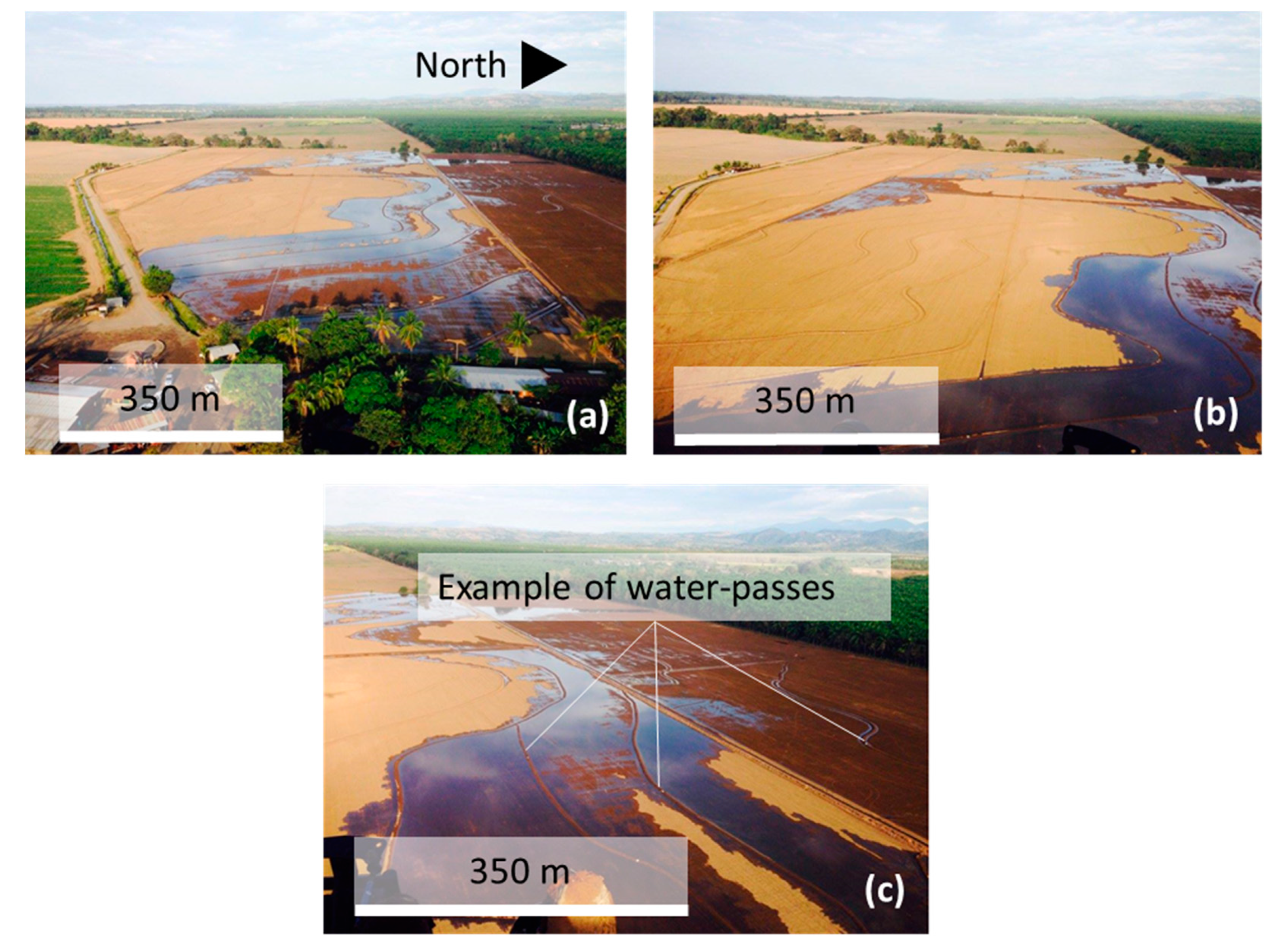
2.1. Environment

The study was conducted in the Central Pacific region of Costa Rica. The field spans approximately 30 ha. The predominant soil type is alluvial Inceptisols [18]. The climate presents two well-defined seasons: a dry season and a rainy season. The dry season ranges from December to March, with April being a transitional month. The rainy season with ≈2500 mm of annual rainfall (around the 40% of it during the growing season), extends generally from May to October, with November as a transitional month. The present study is based on the data from five years (2011–2015) of a rainfed paddy, i.e., cultivated during the rainy seasons; thus, it has the benefits of LL impacting mostly the drainage. Irrigation was not often executed, just during crucial moments when it was required, especially in 2015.

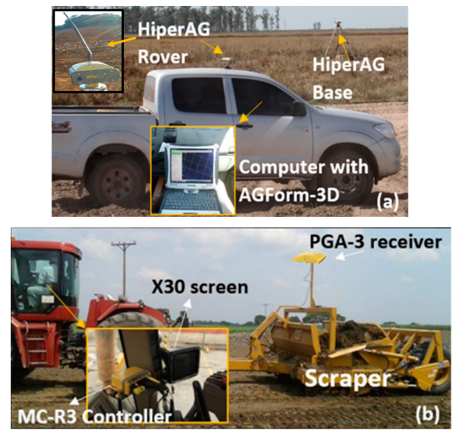
2.2. Land-Leveling Procedures

The process of LL typically involves three main steps, which are: (i) surveying, i.e., a topographic survey of the field; (ii) designing, i.e., the design of an optimal surface; and (iii) grading, i.e., the implementation of the design with tractors and scrapers moving soil. After leveling, frequently, levees with an ellipsoidal smooth surface of about 15–18 cm height and 1.5–2.0 m base-width are created on the field along contours of each 5–10 cm elevation differences. The function of these levees is to facilitate the management of water for irrigation and drainage [8]. Depending on the soil and weather conditions, maintenance actions can be executed in the subsequent years—namely: (i) a topographic survey to check where the designed surface has been altered, and (ii) reparation of points where the levees are broken (e.g., due to the machinery). However, in the studied field such maintenance was not executed, and it was therefore not included in the analysis. An RTK system (Topcon Agriculture; Livermore, California, USA) [19] was used for the field survey in this study. The system consisted of two HiperAG receivers (GPS+GLONASS), one as a base station receiver (“base”) and the other as a rover receiver (“rover”). The base was placed at a fixed point in the field, and the rover mounted on a four-wheel drive vehicle. The average speed of the vehicle during the survey was 5 m/s, and the frequency at which the rover provided RTK solutions was 10 Hz. It is expected that RTK accuracy is 2 cm or less in the horizontal plane (X, Y) and 3 cm or less in height (Z). In the same vehicle, a computer was installed with the AGForm-3D [19] land-leveling software, whose “survey mode” was used to record elevation points in real time. Data points were collected every 5 m along lines spaced about 20 m apart (i.e., at the nodes of an approximately 5 m to 20 m grid), generating a data set with density of 100 points ha⁻¹. For step (2), the “design module” of AGForm-3D was used to create a VS design with an average slop of 0.15% southwestwards, and a maximum cut surface depth of 12 cm at a 1.20 cut/fill ratio factor. Note that AGForm-3D was used for both step (1) and step (2), since it integrates functionalities for both. For step (3), a grading system was used, which automatically controled the hydraulic valves of a scraper during the leveling operation. That grading system was comprised of a GNSS receiver (MC-R3), a GNSS antenna (PGA-3) and a display (X30 computer) installed on the tractor equipped with a scraper. Figure 1 depicts the equipment. The ArcGIS (version 10.2, ESRI, Redlands, California), a geographic information system (GIS), was used to compute and overlap the 3D maps of the original and the leveled topography.

For our analysis we count this operation within the “indirect inputs”—specifically, in the machinery operations. Its economic cost is implicit in the gross amount of investment. Furthermore, in an attempt to reinforce the differences between VS and FS in this manuscript, we computed FS leveling pursuing the planar surface that best fit the original topography of the field. Its main characteristics, such as the total volume of soil removed and the cut depth, were compared with those obtained with the VS design.

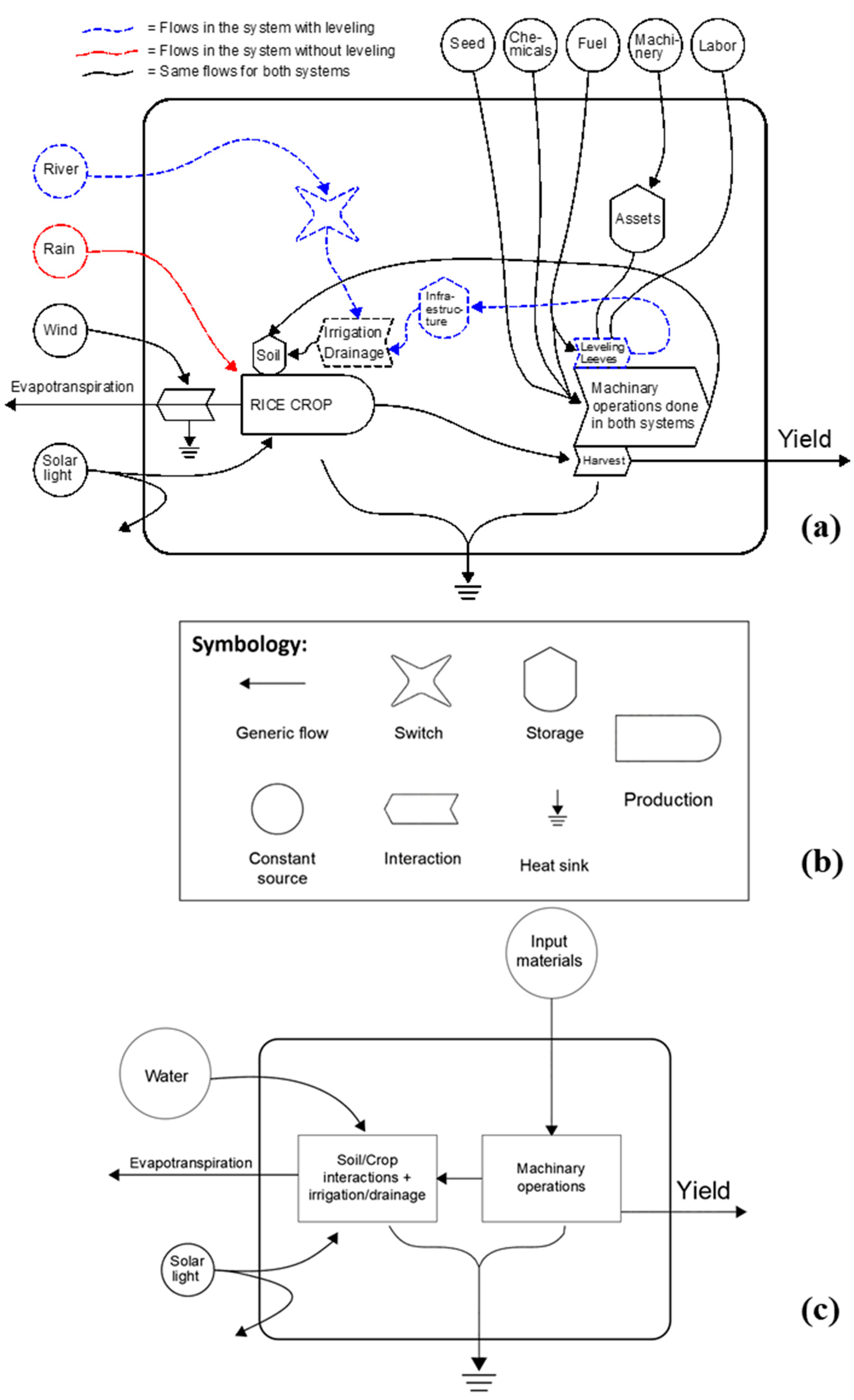
2.3. Material Flow Diagram and Energy Analysis

The material flow diagram of the system herewith analyzed (Figure 2a) is based on terminology suggested by [20]. The symbols are self-explanatory by their names (Figure 2b), except for the switch, which represents paths of energy flow that can be activated and deactivated by human actions. We used that symbol to represent the opening/closing actions in water inlets. The material flow diagram, as a whole, characterizes the path of the energy, since it is included in the system until it leaves. The symbols are used to represent what occurs with the energy within the system—whether it flows, interact with other materials, is stored, is dissipated as heat or is transformed into production (in this case, crop yield). The material flow diagramming involves a set of input data and certain outputs, as described in the following. Input data associated with growing and harvesting a hectare of paddy, including information about seeds, chemicals, fuel, machinery and labor, were obtained directly from the farmer, who also provided the fuel consumption of each operation. In addition, a simplified version of the diagram is presented in Figure 2c, particularly for readers unfamiliar with the illustration of material flows.

In the Figure 2 the interactions of inputs within the system are represented in an energy flow diagram for both scenarios studied, i.e., with and without the implementation of LL. All the acquired inputs (seeds, chemicals, fuel, machinery and labor) are directly related to machinery operations, which improve soil conditions. Obviously, soil quality directly affects the growth of a paddy, which is also influenced by weather conditions—sunlight, rain, wind, etc. Evapotranspiration is represented as a special interaction of climate (wind, sunlight and rain) and the crop. Moreover, the differences between the two systems studied (i.e., one with and one without LL) are represented by different line types. Blue dashed lines show the energy flows present only in the paddy production system with LL, and red dashed lines with arrows show the flows present only on the system without leveling. The continuous lines represent permanent energy flows. These data were converted into energy-per-area using energy equivalents obtained from [21,22] from the Nebraska Trac. Test Lab [14,23]. We calculated the energy required (MJ ha⁻¹) for every input for two scenarios: one with and one without the benefit of land-leveling operations. The primary differences between those two scenarios are due to the addition of costs of machinery operations associated with LL itself and levees marking, and labor. The latter is associated with the labor required for irrigation and drainage, both consisting basically of the same task of opening and closing the water-pass points along the levees (Figure 3). To irrigate the field there is an additional task required: to open/close the water entrance; however, this is a fast and punctual task with a negligible impact on the labor estimations.

Output information was obtained from the yield data of five continuous cropping seasons, from 2011 to 2015, recorded with a gravimetric yield monitor [24], which consisted of a GNSS receiver with sub-meter accuracy, a moisture sensor, a touchscreen console and an impact plate (which indirectly detects the weight of each data point collected). Since only a few farmers in the country used VS-LL, national yield averages were used to show that variations in the production of the study field are not linked to national trends. The original data, in units of Mg ha⁻¹, were converted to units of MJ ha⁻¹ using the equivalence 14,600 MJ Mg⁻¹ ([21]

Table 1. Energy performance of paddy production for both “with leveling” and “without leveling” cases. The respective sources of the embodied energy equivalencies are presented in brackets.

Inputs			Applied (Kg ha−1)	Embodied Energy (MJ kg−1)	Input Energy (MJ ha−1)
					Without Leveling	With Leveling
Direct inputs		Seed	115.00	14.60 [21]	1679.00	1679.00
		Insecticide	28.50	50.00 [23]	1422.50	1422.50
		Herbicide	3.20	90.00 [23]	283.50	283.50
		Fungicide	12.10	50.00 [23]	602.50	602.50
		Bactericide	2.30	50.00 [23]	112.50	112.50
		Fert. N	43.80	73.00 [23]	3199.60	3199.60
		Fert. P2O5	56.40	13.00 [23]	733.30	733.30
		Fert. K2O	64.90	9.00 [23]	584.20	584.20
		Fert. Mg	7.70	10.00 [23]	76.60	76.60
				Subtotal	8693.70	8693.70
Indirect inputs	Labor		Labor (h ha−1)
		Irrigation/drainage	40.00	2.2 [14]	-	88.00
		Weed control	25.00	2.2 [14]	55.00	55.00
		Manual fert.	8.00	2.2 [14]	17.60	17.60
		Other	12.50	2.2 [14]	27.50	27.50
				Subtotal	100.1	188.1
	Machinery		Fuel (L ha1−1)
		Blader roller	8.50	56.30 [22]	478.60	478.60
		Harrowing	6.00	56.30 [22]	337.80	337.80
		Leveling	44.00	56.30 [22]	-	2477.20
		Levee mark	30.00	56.30 [22]	-	1689.00
		Tune up surface	40.00	56.30 [22]	2252.00	2252.00
		Spraying	1.20	56.30 [22]	67.60	67.60
		Sowing	15.00	56.30 [22]	844.50	844.50
		Harvest	20.00	56.30 [22]	1126.00	1126.00
		Fertilization	3.90	56.30 [22]	219.80	219.80
				Subtotal	5326.20	9492.40
				Total input	14,120.00	18,374.20
Outputs			Yield (Mg ha−1)	Embodied Energy (MJ Mg−1)	Input Energy (MJ ha−1)
					Without Leveling	With Leveling
Years		2011	2.80	14,600.00 [21]	40,296.00
		2012	4.42	14,600.00 [21]	64,532.00
		2013	6.09	14,600.00 [21]		88,914.00
		2014	5.40	14,600.00 [21]		78,840.00
		2015	7.50	14,600.00 [21]		109,500.00
				Total output	104,828.00	277,254.00

in Section 3). Data obtained from the yield monitor were processed to generate “yield maps.” In order to analyze the energy performances of the studied systems, the following energy indicators were used (Equations (1)–(3)):

• Energy Return on Investment (EROI) [21,25].

$$EROI=\frac{EO}{EI}$$

(1)

• Energy Productivity (EP) [21,26].

$$EP=\frac{Y}{EI}$$

(2)

• Energy Balance (EB) [21,22,27].

$$EB=EO-EI$$

(3)

The EROI is a unitless index used to represent the amount of energy produced divided by the energy invested; EP is energy productivity, representing the crop produced per unit of energy invested. EP can be computed either as a unitless value if both factors (Y and EI) are converted to MJ ha⁻¹, or as weight (Mg or Kg) per MJ data if Y is not converted. In the present study we calculated the EP in kg MJ⁻¹. EB is energy balance, representing the net energy balance; EO is energy output in units of MJ ha⁻¹; EI is energy input in units of MJ ha⁻¹; and Y is crop yield in units of Mg ha⁻¹. The EI is the sum of the energies contained in all direct (kg ha⁻¹) and indirect (h and L ha⁻¹) inputs, while EO denotes the amount of energy contained in the total grain produced per hectare. To obtain both EI and EO values in terms of MJ ha⁻¹, equivalencies of embodied energy per unit of input and output were utilized (the references are clarified in Table 1).

2.4. Economic Analysis

Our economic analysis quantified the total gain in both scenarios (i.e., with and without LL) by subtracting the amount invested from the partial gain (yield increase times market price). The assumed production cost for a paddy was 2100 USD ha⁻¹ [28,29,30,31]. From 2013 to 2015, it was estimated that the investments in technology, i.e., the cost to acquire the necessary equipment (72,000 USD), depreciated in the total area (400 ha) where said technology was used for over three years of the study. The IT (investment in technology) represents the investment in all the equipment needed for both surveying and leveling; although it can be overestimated due to the short lifespan considered (three years), the investment was 60 USD ha⁻¹. Taken into account as well were the investments in increased machinery use (leveling and levee marking) and labor (irrigation/drainage tasks). A lifespan of 10 years was adopted for the machinery. The partial gain was determined by multiplying additional yield by the market price, 580 USD Mg⁻¹ for all the years [30]. Equations (4) and (5) express how the profit without leveling (PWoL) and the profit with leveling (PWL) were calculated:

$$\mathit{P}\mathit{W}\mathit{o}\mathit{L}\mathbf{=}\frac{\mathit{Y} \mathbf{\times }\mathit{P}}{\mathit{A}}\mathbf{-}\mathit{C}\mathit{P}$$

(4)

$$\mathit{P}\mathit{W}\mathit{L}\mathbf{=}\frac{\mathit{Y} \mathbf{\times }\mathit{P}}{\mathit{A}}\mathbf{-}\mathbf{\left[}\mathit{C}\mathit{P}\mathit{+}\mathit{I}\mathit{T}\mathit{+}\mathit{I}\mathit{M}\mathit{O}\mathit{+}\mathit{I}\mathit{L}\mathbf{\right]}$$

(5)

where Y is the crop yield in Mg, P is the price (USD Mg⁻¹) of one Mg of rice, A is the area of the plot in ha and CP is the cost of production (USD ha⁻¹) for one hectare of paddy. For the estimation of PWL we included IT, IMO (increment in machinery operations) and IL (increment in labor), all expressed in USD. The CP represents agricultural inputs determined by agronomic prescription, such as fertilizers, pesticides and seeds. Investment in machinery operations (IMO) for LL was obtained based on 230 USD ha⁻¹. For every hectare, around 120 m³ of soil was moved, resulting in a cost of about 1.9 USD m⁻³. Investment in labor (IL) was also based on the farmer’s records—considered the same as the cost for irrigation management; it totaled 140 USD ha⁻¹ which was the only additional labor after land forming.

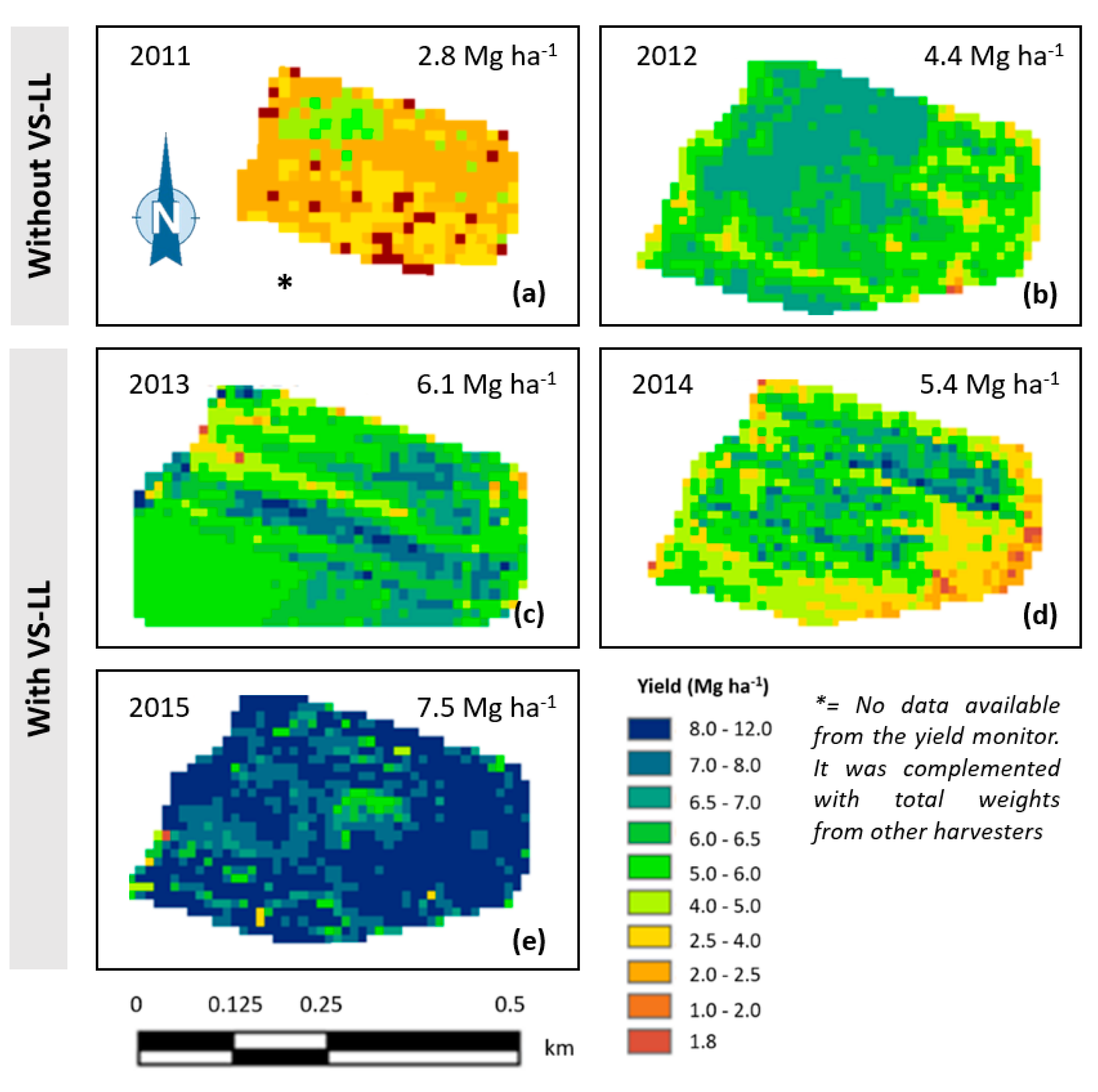
3. Results and Discussion

The surfaces depicted in the following figure were generated from surveys and VS leveling designs using AGForm-3D. The original (Figure 4a) and leveled (Figure 4b) surfaces are presented alongside the map of cuts and fills carried out (Figure 4c). In an attempt to reinforce the differences between the VS 3D-land forming and the FS best-fitting plane leveling, previously reported by [6], we estimated how much the maximum cut depth and volume of soil removed would be if the FS was employed. The results showed that the volume of soil to be removed with the FS would be 450 m³ ha⁻¹, i.e., around 3.75 times more compared with the VS (120 m³ ha⁻¹, as reported in Section 2). Moreover, the depths of cuts and fills in the VS design were always lower than 20 cm (distributed in site specific spots of a few square meters), whereas the FS design resulted in cuts and fills exceeding 45 cm (distributed larger areas of several hundred square meters). Obviously, our choice of a VS design surface in this case fulfills our objective to minimize topsoil disturbance, compared to the alternative FS design surface.

Figure 5 shows yield maps for the harvest periods evaluated. LL was conducted only in years 2013, 2014 and 2015. The lowest yield in the five-year study was observed in 2011, before LL commenced, when the average was 2.76 Mg ha⁻¹. In 2012, the average increased to 4.42 Mg ha⁻¹, but it was still lower than the yields obtained in 2013–2015 when LL was performed. In 2013, after implementing leveling, the yield increased by more than 3 Mg ha⁻¹ compared to 2011 and more than 1.5 Mg ha⁻¹ compared to 2012. Consequently, technological adoption alone does not guarantee against yield decrease. Rather, combining LL with good practices such as selection of a quality seed hybrid and an appropriate planting density [10] should result in a higher probability of avoiding yield decreases. We assert that LL creates conditions more favorable for the inputs and that is should be expected to result in a more homogeneous growth of the crop.

The impacts of LL on crop production were analyzed considering biotic and abiotic stress conditions of particular seasons. For that purpose, field records of crop health, and historical records about the occurrence of El Niño and La Niña climatic phenomena offer an idea about stress environments in specific years. Figure 6a presents the Oceanic Niño Index (ONI, National Oceanic and Atmospheric Administration—NOAA) [32] used to monitor the El Niño-Southern Oscillation (ENSO), namely, the presence of either of the two phenomena (Figure 6b) during the period of the study (2011–2015). The figure includes the national and the field study average yields as well (Figure 6c).

In 2011, La Niña caused rainier and cooler weather, which alongside the lack of levees to drain the field and suboptimal microrelief, might be associated with the lower average yield of the study field compared with the Costa Rican mean. During 2012–2013, at neutral to transitional ENSO phases, and without a meaningful biotic stress, the effect of LL on production is clearer. The yield increased from 4.42 Mg ha⁻¹ in 2012 to 6.09 Mg ha⁻¹ in 2013 (first year with leveling). In 2014, aside from weather factors promoted by the El Niño in the second half of that year, the decrease in crop yield is attributed to a rice mite (Steneotarsonemus spinki) attack. In 2015, with a more intense El Niño effect but without meaningful biotic stress, the average yield in the study field surpassed two times the national mean; meaning that such a production increase was not linked to a general trend in the country. This finding highlights the greater impact of LL when the capacity to manage precision irrigation and drainage becomes crucial to keep a crop healthy, under adverse weather conditions. Specifically, in 2015, there was a combined effect of the LL benefits, which was used (i) to improve the water retention within the field by closing the water-passes when precipitation rates declined, and (ii) to execute some irrigation events when they were necessary due to the stronger El Niño effect.

In a parallel study, Quiros et al. [32] analyzed the effect of LL on the distribution of yield homogeneous zones. In 2013, in a contiguous rainfed paddy field without LL, the authors reported a yield 3.79 Mg ha⁻¹ lower than the one measured in the present study (already with LL by that time). Remarkably, in 2014 when the field analyzed in the [33] research was leveled, its yield (5.10 Mg ha⁻¹) was similar to the one observed in the present study (5.40 Mg ha⁻¹). Moreover, in 2015 the yield increased by around 2.90 Mg ha⁻¹ in both studies. These results offer an idea about the consistency in the impact of LL on the yield, particularly in 2015 when LL was used for both irrigation and drainage purposes.

Besides the quantitative impacts on yield, our investigation addresses the flow of materials within the paddy system as well (Figure 2, Section 3). The diagram describes how the input energy coming from constant external sources, such as seeds, chemicals and fuel, interacts with the machinery operations done in both systems, and its embodied energy finally converges in the crop land. Some fuel is invested for leveling and levees marking operations and some of its energy is stored in the new infrastructure (levees), and some other amount of energy is required by irrigation. Part of the remaining energy was used to provide inputs into the soil, which provides together rain (in systems without leveling), river water (only in systems with leveling), solar light and the evapotranspiration (as an interaction which liberates water from the system as well) conditions to rice production in the paddy crop until harvest. Finally, some heat comes out from the harvest operation to obtain the yield as the final output. As a final annotation, the energy flow arrow of the sunlight that comes immediately out of the system represents the solar light reflected by the canopy.

All the inputs required and all the energy the paddy produced are listed for both systems: with and without leveling (Table 1). Direct inputs represent the same amount of energy in both scenarios, because the amounts of seeds and chemicals required do not depend on whether LL is done or not. The energy demand was 8.69 GJ ha⁻¹, of which seed and nitrogen comprise the highest values. On the other hand, indirect inputs varied from 5.33 GJ ha⁻¹ without leveling to 9.49 GJ ha⁻¹ with leveling. This difference was due to the increase of machinery use for leveling. In this study, energy output is considered as the amount of energy per amount of the grain harvested. Following [21] a value of 14,600.00 MJ Mg⁻¹ was adopted.

To better understand the benefits of technology adoption, in terms of energy conserved, the use of certain energy indices for the inputs and outputs is most helpful.

Table 2. Energy indices computed for each year of the study.

Status	Year	Index
		EROI	EP (kg MJ−1)	EB (MJ ha−1)
Not leveled	2011	2.85	0.19	26,192.00
	2012	4.57	0.31	50,412.00
Leveled	2013	4.84	0.33	70,580.00
	2014	4.29	0.29	60,506.00
	2015	5.96	0.41	91,166.00

shows the values of three energy indices calculated for each year of the study: energy return on investment (EROI), energy productivity (EP) and energy balance (EB). EROI is computed as a ratio of the amount of energy produced to the amount of energy invested. For example, an EROI value of 1 means that the amount of energy invested was the same as the amount of energy produced, whereas a value greater than 1 means that there was more energy produced than invested. Considering the general improvement that leveling resulted in, 2014 was an exception for EROI and EP (both 7% lower than in 2012). In the same season, EB was 20% above 2012. For both 2013 and 2015, EROI and EP were 5% to ≈30% above 2012, respectively, whereas the EB values for 2013 and 2015 were 20% and 80% above that of 2012, respectively. Averaged index values for the scenarios leveled and non-leveled show that leveling has a 93.3% improvement in EB and 35.5% improvements in EROI and EP, respectively, compared to the non-leveled case. Note that EROI and EP represent the same trend, since output energy is directly proportional to yield.

The higher yield, EP, ER and EB values in 2015, compared to 2013 and 2014, suggest that the benefit of LL may increase over time, which would be an argument in its favor as a partial solution to the growing demand to conserve energy in paddy production [4,35]. The additional energy demand (4254 MJ ha⁻¹) is equivalent to 0.29 Mg ha⁻¹ of paddy, which is the minimum additional yield to keep the same EB.

Finally, an economic analysis can also help to decide for or against technology adoption (GNSS-controlled LL in this case). Thus, we present

Table 3. Economic analysis comparing the investment partial and total gains of the scenarios with and without LL.

Year		Investment (USD)				Partial Gain			Total Gain (USD)
		CP *	IT *	IMO *	IL *	Yield (Mg)	Price (USD Mg−1)	(USD ha−1)
Not leveled *	2011	2100				2.76	580	1601	−499
	2012	2100				4.42	580	2564	464
Leveled **	2013	2100	60	230	140	6.09	580	3532	1002
	2014	2100	60	230	140	5.40	580	3132	602
	2015	2100	60	230	140	7.50	580	4350	1820

* Calculated based on the PWoL (Equation (4)); ** calculated based on the PWL (Equation (5)).

, which shows the resulting profit in the field for each of the five years of study. The negative value of profit in 2011 was due to low income caused by a low yield. From 2013 to 2015, after leveling was performed, the investment cost was 2530 USD ha⁻¹, being the sum of CP (2100 USD ha⁻¹), IT (60 USD ha⁻¹), IMO (230 USD ha⁻¹) and IL (140 USD ha⁻¹). Income is the result of yield multiplied by the paddy price (580 USD Mg⁻¹), which was considered fixed for all five years.

After leveling, the average profit was 3.4 times higher than 2012 (from 2.3 to 4.9). We did not consider 2011 when making these comparisons, as its unexpectedly low total gain could overestimate the benefits of technological adoption (here, LL). Indeed, a longer-term analysis could prove more reliable, but decisions on whether to adopt new technology cannot always wait. Often, when technological options are introduced into the market, farmers have no reliable way to judge the degree of their benefit. The results suggest that, for the technology evaluated here, and even with the lower yield of 2014, the investment was worth it. The additional production cost of 430 USD ha⁻¹ (i.e., IT+IMO+IL) is equivalent to 0.74 Mg ha⁻¹ of paddy, which was the minimum additional yield to keep the same profit realized in 2012 before LL was performed.

Alongside the energy performance and economic profitability, the ecological benefit of the GNSS/RTK-based VS-LL might be highlighted from two perspectives: (i) the higher efficiency in the use of water, and (ii) the shallower soil alteration. Such technology which improves irrigation and drainage efficiencies may help in the feasibility of producing crops in water-scarce regions. Given the current generalized water scarcity around the world [36], it might be helpful in a wide range of crops and regions, especially those crucial for the food safety of vulnerable populations. For instance, Sub-Saharan African crops are in need of these techniques to improve production systems, in a context where the access to food is increasingly difficult, and the lack of technology makes it difficult to access the sources of water in their arid to semi-arid climate [37]. Abdullaev et al. [38], for instance, reported a reduction of more than 500 m³ ha⁻¹ in the water application rate in fields leveled by laser. A similar impact would be expected with VS leveling, without the large soil displacement commonly seen in laser leveling. Moreover, by means of the shallower cuts and fills, the GNSS/RTK-based VS-LL is suitable for soil conservation. This is a critical fact in the present context where soil is being degraded by human actions and land use changes, and again, the least advanced economies (Sub-Saharan Africa, South America and South Asia) are the most affected [39].

The impact of the LL on the yield in the studied rainfed paddy field is directly attributed to the improved drainage. With the field leveled and levees built the farmer was able to: (i) release the excess of water within the field during, e.g., either days of higher precipitation or specific phenologies which require drier soil, and (ii) retain the water in the field during days of lower rainfall. Indirectly, LL improves the homogeneous availability of water for the crop [3], at the time that facilitates a more efficient control of weeds, and a greater efficiency in nutrient uptake [4]. Besides the commented-on benefits of LL for crop production, a set of limitations associated with the LL operation, in general (not VS specific), have to be mentioned. First, considering the risk of removing the topsoil layer, its depth must be considered before executing the operationm in the sense that the maximum cut designed must be several centimeters shallower than the topsoil. In addition, the field size should be accounted for in the designs as well, avoiding long soil carrying distances and deeper and larger cut and fill areas; for instance, large fields (in the order of several tens of hectares) should be divided into smaller ones where the cut and fills can be better distributed. Moreover, the price of LL equipment (specified above) is sometimes a limitation for farmers, depending on their production capacity; however, at the same time it presents an opportunity for companies to develop outsourcing businesses.

4. Conclusions

The implementation of LL-VS positively impacted the sustainability performance in the studied paddy field. Improvements of yield and energy performance were detected after the adoption of VS-LL. The impact of LL on yield is stronger under adverse weather conditions with irregular water supply, either limited or excessive. In such situations the precision irrigation (in dry seasons) and drainage (in rainy seasons) management enabled by LL becomes crucial to keep a crop productive. Furthermore, our analysis has shown that the technological adoption of VS-LL resulted in gains of energy efficiency and crop profitability. In average results, the additional energy demand (4254.00 MJ ha⁻¹) was compensated by higher additional energy output, providing greater EROI, EP and EB. Moreover, the augment in the return of energy obtained by implementing the VS leveling surpasses the increase in input energy that it requires, since the increase in energy output in the form of yield is higher than the increase of indirect inputs. Indeed, the energy compensation is reached with additional yield above 0.29 Mg ha⁻¹, over the one obtained without land forming. In addition, from the economic perspective, after leveling the average profit was 3.4 even with the lower yield of 2014. Therefore, this suggests that the VS was worth the investment for the field and the conditions of the present study. Finally, environmental benefits should also be noted, since VS allowed shallower topsoil cuts distributed on specific spots. Indeed, the implementation of said operation brings the production benefits of a more efficient irrigation system, while at the time that avoiding major damage to topsoil layers.

References

1. Jat, M.L.; Gupta, R.; Ramasundaram, P.; Gathala, M.; Sidhu, H.S.; Singh, S.; Singh, R.; Saharawat, Y.; Kumar, V.; Chandna, P.; et al. Laser-assisted precision LL: A potential technology for resource conservation in irrigated intensive production systems of Indo-Gangetic Plains. In Integrated Crop and Resource Management in the Paddy-Wheat System of South Asia; Ladha, J.K., Singh, Y., Eds.; International Rice Research Institute (IRRI): Los Bolaños, Philippines, 2009; pp. 223–237. [Google Scholar]
2. Khan, F.; Khan, S.U.; Sarir, M.S.; Khattak, R.A. Effect of LL on some physico-chemical properties of soil in district DIR lower. Sarhad J. Agric. 2007, 23, 107–114. [Google Scholar]
3. Bouman, B.A.M.; Hengsdijk, H.; Hardy, B.; Bindraban, P.; Tuong, P.; Ladha, J.K. Water-Wise Paddy Production; International Rice Research Institute (IRRI): Los Bolaños, Philippines, 2002; 356p. [Google Scholar]
4. Chauhan, B.S. Weed Management in Direct-Seeded Rice Systems; International Rice Research Institute (IRRI): Los Bolaños, Philippines, 2012; 20p. [Google Scholar]
5. Bueno, M.V.; de Campos, A.D.S.; da Silva, J.T.; Massey, J.; Timm, L.C.; Faria, L.C.; Roel, A.; Parafit, J.M.B. Improving the Drainage and Irrigation Efficiency of Lowland Soils: Land-Forming Options for Southern Brazil. J. Irrig. Drain Eng. 2020, 146, 04020019. [Google Scholar] [CrossRef]
6. Quiros, J.J.; Aguero, J.A.; Fiorio, P.R. Melhoramento da drenagem através da técnica de nivelamento por declividade variável em uma área de algodão com o sistema GNSS-RTK_AGForm-3D. In Proceedings of the XLIV Brazilian Congress of Agricultural Engineering, Sao Pedro-SP, Brazil, 13–17 September 2015. [Google Scholar]
7. Quiros, J.; Winkler, A.S.; Aguero, J.; Tavares, T.R.; Martello, M. Efeito da sistematização por declividade variável no microrrelevo de talhão cultivado com arroz no pacífico central da Costa Rica. In Proceedings of the Brazilian Congress of Precision Agriculture, Goiânia, Brasil, 4–6 October 2016. [Google Scholar]
8. Quiros, J.; Winkler, A.; Aguero, J. Avaliação do desempenho da marcação de taipas com um sistema de direção automática assistida. In Proceedings of the X Brazilian Congress of Irrigated Rice, Gramado-RS, Brazil, 8–11 August 2017. [Google Scholar]
9. Sowell, R.S.; Shih, S.F.; Kriz, G.J. Land forming design by linear programming. Trans. ASABE 1973, 16, 296–301. [Google Scholar] [CrossRef]
10. Aquino, L.S.; Timm, L.C.; Reichardt, K.; Barbosa, E.P.; Parfitt, J.M.B.; Nebel, A.L.C.; Penning, L.H. State-space approach to evaluate effects of land levelling on the spatial relationships of soil properties of a lowland area. Soil Till. Res. 2015, 145, 135–147. [Google Scholar] [CrossRef]
11. Perryman, M.E.; Schramski, J.R. Evaluating the relationship between natural resource management and agriculture using embodied energy and eco-exergy analyses: A comparative study of nine countries. Ecol. Complex. 2015, 22, 152–161. [Google Scholar] [CrossRef]
12. Bora, G.C.; Nowatzki, J.F.; Roberts, D.C. Energy savings by adopting precision agriculture in rural USA. Energy Sustain. Soc. 2012, 2, 5. [Google Scholar] [CrossRef] [Green Version]
13. Brown, M.T. A picture is worth a thousand words: Energy systems language and simulation. Ecol. Model. 2004, 178, 83–100. [Google Scholar] [CrossRef]
14. Romanelli, T.L.; Milan, M. Material flow determination through agricultural machinery management. Sci. Agric. 2010, 67, 375–383. [Google Scholar] [CrossRef] [Green Version]
15. Spekken, M.; de Bruin, S. Optimized routing on agricultural fields by minimizing maneuvering and servicing time. Precis. Agric. 2013, 14, 224–244. [Google Scholar] [CrossRef]
16. Spekken, M.; Molin, J.P.; Romanelli, T.L. Cost of boundary manoeuvres in sugarcane production. Biosyst. Eng. 2015, 129, 112–126. [Google Scholar] [CrossRef]
17. Colaço, A.F.; Povh, F.P.; Molin, J.P.; Romanelli, T.L. Energy assessment for variable rate nitrogen application. Agric. Eng. Int. CIGR J. 2012, 14, 85–89. [Google Scholar]
18. Monge, L.A.; Alvardo, A. Caracterización y clasificación de los principales suelos del Valle de Parrita. Argon. Costarr. 1979, 3, 123–128. [Google Scholar]
19. Topcon Agriculture. Available online: https://www.topconpositioning.com/agriculture (accessed on 8 July 2020).
20. Odum, H.T. Environmental Accounting: Emergy and Environmental Decision Making, 1st ed.; Wiley: Hoboken, NJ, USA, 1996; p. 359. [Google Scholar]
21. Eskandari, H.; Attar, S. Energy comparison of two paddy cultivation systems. Renew. Sustain. Energy Rev. 2015, 42, 666–671. [Google Scholar] [CrossRef]
22. Rathke, G.W.; Wienhold, B.J.; Wilhelm, W.W.; Diepenbrock, W. Tillage and rotation effect on corn-soybean energy balances in eastern Nebraska. Soil Till. Res. 2007, 97, 60–70. [Google Scholar] [CrossRef] [Green Version]
23. Pellizzi, G. Use of energy and labour in Italian agriculture. J. Agric. Eng. Res. 1992, 52, 111–119. [Google Scholar] [CrossRef]
24. AgLeader. Available online: https://www.agleader.com (accessed on 8 July 2020).
25. Atlason, R.; Unnthorsson, R. Ideal EROI (energy return on investment) deepens the understanding of energy systems. Energy 2014, 67, 241–245. [Google Scholar] [CrossRef]
26. Brar, A.S.; Buttar, G.S.; Jhanji, D.; Sharma, N.; Vashist, K.K.; Mahal, S.S.; Deol, J.S.; Singh, G. Water productivity, energy and economic analysis of transplanting methods with different irrigation regimes in Basmati paddy (Oryza sativa L.) under north-western India. Agric. Water Manag. 2015, 158, 189–195. [Google Scholar] [CrossRef]
27. Valentas, K.; Singh, R.P.; Rotstein, E. Handbook of Food Engineering Practice; CRC Press: Boca Raton, FL, USA, 1997. [Google Scholar] [CrossRef]
28. Corporación Arrocera Nacional (CONARROZ). Statistical Report, 2011–2012. 2012. Available online: https://www.conarroz.com/estadisticasarroceras.php (accessed on 8 July 2020).
29. Corporación Arrocera Nacional (CONARROZ). Statistical Report, 2012–2013. 2013. Available online: https://www.conarroz.com/estadisticasarroceras.php (accessed on 8 July 2020).
30. Corporación Arrocera Nacional (CONARROZ). Statistical Report, 2013–2014. 2014. Available online: https://www.conarroz.com/estadisticasarroceras.php (accessed on 8 July 2020).
31. Corporación Arrocera Nacional (CONARROZ). Statistical Report, 2012–2015. 2015. Available online: https://www.conarroz.com/estadisticasarroceras.php (accessed on 8 July 2020).
32. National Oceanic and Atmospheric Administration (NOAA). Cold & Warm Episodes by Season. Available online: https://origin.cpc.ncep.noaa.gov/products/analysis_monitoring/ensostuff/ONI_v5.php (accessed on 19 August 2020).
33. Quiros, J.; Winkler, A.S.; Aguero, J.; Tavares, T.R.; Martello, M. Efeito da sistematização sobre a produtividade e distribuição de unidades de gestão diferenciada em um campo cultivado com arroz (Oriza sativa). In Proceedings of the Brazilian Congress of Precision Agriculture, Goiânia, Brasil, 4–6 October 2016. [Google Scholar]
34. National Meteorological Institute of Costa Rica (IMN). Boletín ENOS. Available online: https://www.imn.ac.cr/boletin-enos (accessed on 19 August 2020).
35. Khoshnevisan, B.; Rajaeifar, M.A.; Clark, S.; Shamahirband, S.; Anuar, N.B.; Shuib, N.L.M.; Gani, A. Evaluation of traditional and consolidated paddy farms in Guilan Province, Iran, using life cycle assessment and fuzzy modeling. Sci. Total. Environ. 2014, 481, 242–251. [Google Scholar] [CrossRef] [PubMed]
36. Food and Agriculture Organization (FAO). Water Scarcity—One of the Greatest Challenges of Our Time. Available online: http://www.fao.org/fao-stories/article/en/c/1185405/ (accessed on 18 August 2020).
37. Food and Agriculture Organization (FAO). Resources and Challenges in the Context of Climate Change. Available online: http://www.fao.org/3/i2345e/i2345e04.pdf (accessed on 18 August 2020).
38. Abdullaev, I.; Hassan, M.U.; Jumaboev, K. Water saving and economic impacts of LL: The case study of cotton production in Tajikistan. Irrig. Drain. Syst. 2007, 21, 251–263. [Google Scholar] [CrossRef]
39. Borrelli, P.; Robinson, D.A.; Fleischer, L.R.; Lugato, E.; Ballabio, C.; Alewell, C.; Meusburger, K.; Modugno, S.; Schütt, B.; Ferro, V.; et al. An assessment of the global impact of 21st century land use change on soil erosion. Nat. Commun. 2017, 8, 1–13. [Google Scholar] [CrossRef] [PubMed] [Green Version]
Figure 1. Field equipment and machinery: GNSS-RTK system for (a) topographic survey and (b) land leveling (LL).
Agronomy 10 01681 g001
Figure 2. Material flows in LL and non-leveling systems, both with specific line types: blue dashed lines for flows for the leveled scenario; red dashed lines for the flows in the systems without leveling. Continuous lines represent permanent energy flows (a). The symbols and terminology (b) are based on [20], presented by [14] as well. In (c) a simplified version of the diagram is presented for readers unfamiliar with the illustration of material flows.
Agronomy 10 01681 g002
Figure 3. Aerial perspective of the study field during irrigation in 2016 (a,b), and a zoom-in exemplifying where some water-passes were located (c). Pictures are included for illustration purposes; no similar pictures are available for the years of the study.
Agronomy 10 01681 g003
Figure 4. 3D surfaces of (a) original topography, (b) VS leveled topography and (c) the respective map of cuts and fills. The contour lines in (b) represent the pattern of the levees that were marked on field after the executing the VS design.
Agronomy 10 01681 g004
Figure 5. Yield maps based on the information obtained from the yield monitoring system [24] for the harvest periods 2011–2015. The labels on the left-hand side indicate the years without (a,b) and with (ce) VS-LL. The average yield is presented at the top right of each map. A common color scale was used for the four maps.
Agronomy 10 01681 g005
Figure 6. Monthly intensity of El Niño and La Niña according to the Oceanic Niño Index (ONI, National Oceanic and Atmospheric Administration—NOAA) [31] (a); locally reported El Niño and La Niña phases regarding the El Niño-Southern Oscillation (ENSO, National Meteorological Institute of Costa Rica—IMN) [34] (b); and yearly average yields in the country and the study field (c) [28,29,30,31].
Agronomy 10 01681 g006