Autowave Physics of Material Plasticity

Abstract

The notions of plastic flow localization are outlined in the paper. It is shown that each type of localized plasticity pattern corresponds to a definite stage of deformation hardening. In the course of plastic flow development, a changeover in the types of localization patterns occurs. The types of localization patterns are limited in number: four pattern types are all that can be expected. A correspondence was set up between the emergent localization pattern and the respective flow stage. It is found that the localization patterns are manifestations of the autowave nature of plastic flow localization process, with each pattern type corresponding to a definite mode of autowave. In the course of plastic flow development, the following modes of autowaves will form in the following sequence: switching autowave → phase autowave → stationary dissipative structure → collapse of the autowave. Of particular interest are the phase autowave and the respective pattern observed. Propagation velocity, dispersion, and grain size dependence of wavelength were determined experimentally for the phase autowave. An elastic-plastic strain invariant was also introduced to relate the elastic and plastic properties of the deforming medium. It is found that the autowave characteristics follow directly from this invariant.

1. Introduction

Almost 200-year-old history of scientific research of the nature of plastic deformation in solids has not yet led to a complete understanding of this problem, but has elucidated limitations of mechanical and physical approaches to it. Thus, the mechanics of plasticity is characterized by a variety of employed macroscale models (e.g., see [1,2,3]), often very simplified. They quite often have only a pragmatic substantiation and are focused on solving particular problems of plastic deformation. Within the framework of these approaches, narrow practical aims can be achieved, obviously insufficient for understanding of the nature of plasticity phenomenon.

Physical (usually dislocation) models of plasticity [4,5,6] are mostly based on an electron microscopic analysis of small volumes of a deformed crystal [7]. Microstructural data obtained in these cases are extrapolated without doubt to a macroscopic volume; generally speaking, this is not always well substantiated.

In 1987 Seeger and Frank [8] proposed to consider plastic deformation as a process of structurization stating that “the use of thermodynamics of irreversible processes in open systems to a description of structurization during plastic deformation of crystal materials is quite promising on qualitative level.” This idea opened the way to application of synergetic methods in physics of plasticity [9,10,11,12]. The attractiveness of this idea was explained by the well-known progress in understanding of the nature of functioning of alive organisms [13,14,15] provided by this science.

However, the use of the synergetics approach requires a realistic description of a deforming medium taking into account such its properties as:

- Openness providing energy exchange between the sample and the testing machine [16],

- Nonlinearity [17] on the macroscopic level in the form of the strain–stress curve $\sigma \left(\epsilon \right)$ and on the dislocation level in the complex character of the strain–stress interaction during deformation [4,5,6],

- Inhomogeneity due to the presence of crystal defects, internal stresses, and other deviations from ideal crystal structure that can, according to synergetics principles, lead to self-organization of the structure [9,10,11],

- Activity of the deforming medium determined by the presence of potential energy sources (elastic stress concentrators) distributed over the volume [5,18], which can relax during deformation, generating lattice defects,

- Irreversibility of plastic deformation, i.e., impossibility of restoration of initial structure and properties after removal of loading because of lattice defect generation [5,18].

The above consideration translates the deforming medium to the class of objects whose dynamics should be described within the frames of synergetics [9,10,11,12,13,14,15]. Authors of [10] pointed out that “it is impossible to investigate so important and widespread mechanical phenomena as plasticity and fluidity on purely mechanical basis; instead, they should be considered as a part of the general subject area of nonlinear dynamic systems operating far from resonance”.

This explains current interest to the study of the plasticity problem within the framework of a more general problem of the behavior of a substance far from the equilibrium state. A similar approach, which is new for synergetics, can be useful for other fields of science, since plastic deformation is a response of an open nonequilibrium system on external action that can be investigated comparatively easily. It is important that the microscopic aspect of the problem has been studied much better than the macroscopic one (for example, see [4,5,6,7,19,20,21]).

2. Experimental Basis of the New Approach

It is natural to start general analysis of structurization from very important statement of authors [22] that “structurization in an open nonlinear medium is associated with the effect of localization.”

2.1. Hypothesis about Plastic Flow Localization

This statement is applicable to plastic deformation during which initially homogeneous medium is spontaneously separated into deforming and nondeforming zones (nuclei) whose boundaries can move. Deformation starts from nucleation of the Lüders band during elastoplastic transition [11] and ends by formation of a failure neck. It is reasonable to assume that plastic flow at intermediate stages is also macroscopically localized, and the lack of data is caused by disadvantages of experimental procedures used to record a plastic flow.

These considerations have allowed us to hypothesize in [23] that macroscopic localization is a general distinguishing characteristic of plastic deformation process accompanying it from elastoplastic transition to failure. The application of the localization phenomenon in analysis of plasticity means transition to geometrical description of the problem. In this case, the process is characterized by shapes of localized plasticity nuclei, volume localization, velocity, and character of their motion, etc. The localization pattern forms a deformation structure in the sense prescribed in [8]; correct explanation of the nature of plasticity is impossible without its analysis.

2.2. Plastic Strain Localization Patterns

The correctness of the suggested hypothesis was confirmed by numerous experiments on plastic deformation of different materials by different mechanisms. To observe localization patterns, the method combining mechanical tests with double-exposure speckle photography adapted for plastic deformation was used [24,25]. This allowed to reconstruct the displacements vector field $\mathbf{r}\left(x,y\right)$ arising on the flat sample surface for step-by-step strain increase by $\delta \epsilon \approx {10}^{-3}$ at any stage of the process and the components of plastic distortion tensor [1]

$${\beta }_{ij}=\nabla \mathbf{r}\left(x,y\right)={\epsilon }_{ij}+{\omega }_z=\left(\begin{array}{cc}{\epsilon }_{xx}& {\epsilon }_{xy}\\ {\epsilon }_{yx}& {\epsilon }_{yy}\end{array}\right)+{\omega }_z$$

(1)

to be calculated. Figure 1a–d shows dependences of the plastic strain tensor component ${\epsilon }_{xx}$ in the samples, referred to as the localized strain patterns. The behavior of the components of the tensor (1) can be analyzed using the X-t diagrams (dependences of the deformation nucleus coordinates X on time t). They allow to measure the spatial, λ, and temporal, T, periods of the process, as it is shown, for example, in Figure 2b. Then the wave number $k=2\pi /\lambda$, the frequency $\omega =2\pi /T$, and the motion rate of the deformation nucleus $V_{aw}=\lambda /T=\omega /k$ are calculated.

To elucidate the meaning of the pattern, the relative strain increment $\delta \epsilon$ between two exposures can be estimated as

$$\delta \epsilon \approx \frac{\delta L}{L}\approx \frac{{\displaystyle \sum _{i=1}^N{\left({\epsilon }_{xx}^{(mag)}\right)}_i{l}_i}}{L}\approx \frac{N\cdot \langle {\epsilon }_{xx}l\rangle }{L},$$

(2)

where N is the number of localized active flow nuclei with size l in the pattern, ${\epsilon }_{xx}^{(mag)}$ is the amplitude of the plastic strain tensor component ${\epsilon }_{xx}$ in such nuclei, $\langle {\epsilon }_{xx}l\rangle$ is the average elongation within the nucleus, and $L>Nl$ is the sample length. Verification of Equation (2) showed that the total strain is actually the sum of strains in active nuclei, i.e., the events in localization zones are more impor­tant than the events in zones between them that, in principle, can be neglected.

Over the last few years, the existence of the localized plastic flow patterns has been independently confirmed by a number of authors (for example, see [26,27,28,29,30,31]). The use of laser interferometry, methods of correlation of digital surface images, and thermal vision systems in these investigations has confirmed the correctness of the hypothesis about the universal character of plastic flow localization formulated above. These patterns are characteristics for the macroscopic observations of plasticity phenomena only.

2.3. Plastic Flow as an Autowave Process

Evidence of the existence of localized plastic flow patterns and data on their temporal dynamics have forced researchers to understand that an explanation of the observable patterns should be based on the notion of periodic spatiotemporal processes on the macroscopic levels. This can be explained, at least, by two ways.

First of all, it is well known that the so-called the Kolsky stress waves [32] are formed during elastoplastic transition in deforming materials. Experimentally, they were studied in detail in [33,34]. Hähner used this point of view and considered dislocation reactions on the Lüders front as a wave process analogous to the Kolsky stress waves [35].

On the other hand, simultaneously, in our work [36] the autowave representations were suggested. The autowaves are generated in active media spontaneously [34]. The choice between waves and autowaves was determined further by three arguments. The first consisted in the difference between the velocities of the Kolsky stress waves $10\le V_K\left(\theta \right)\approx \sqrt{\theta /{\rho }_0}\le {10}^2$ m/s ($\theta =d\sigma /d\epsilon$) is the work hardening coefficient and ${\rho }_0$ is the material density) [32,33] and the investigated processes ${10}^{-5}\le V_{aw}\le {10}^{-4}$ m/s. The ratio $V_K/V_{aw}\approx {10}^5-{10}^7$ excluded reduction of the observable localization processes to the Kolsky stress waves.

The second argument is the difference between the mechanisms of initiation of waves and autowaves. To excite a wave process, an external impact is necessary, whereas an autowave process is engendered by internal interactions of elements of the active medium [34]. From representations about the mechanical method of material testing it is clear that loading is quasi-static in character, so that the autowave localization nature is preferable.

Finally, the third argument in favor of the autowave is that the forms of the Kolsky stress waves are reduced actually only to propagation of solitary deformation fronts [33]. At the same time, the autowaves form different modes [34] corresponding to different experimental patterns of localized plasticity. Taken together, considerations above led to the opinion that the examined spatiotemporal processes can be viewed as the localized plastic flow autowaves [25].

2.4. Patterns. Autowaves. Work Hardening Stages

Investigations performed in [35,36,37,38,39,40,41] showed that geometrically the localized plasticity pattern is the cross section of the volume autowave mode by the observable sample surface. To understand the nature of the phenomenon, it is important to compare the observable patterns with stages of work hardening [5,6] that can be seen on the flow curve $\sigma \left(\epsilon \right)$ or on the dependences $\theta \left(\epsilon \right)$ [6,42].

It turns out that there is a one-to-one correspondence between the stages and patterns. This is illustrated by the X-t diagrams in Figure 2a–d. Thus, for the yield plateau stage with $\sigma \approx const$ and $\theta \approx 0$, the localized plasticity pattern depicts motion of the single nucleus (Figure 2a) known as the Lüders band [11]. On its front, the elastic medium is transformed into the plastically deforming state with different structure and work hardening mechanisms.

The stage of linear work hardening with $\sigma ~\epsilon$ and $\theta \approx const$ is determined by the interaction and multiplication of dislocation [5,35]. In this case, the strain nuclei can be repeatedly excited in the same volumes of the material with time intervals determined by the properties and the state of the medium (Figure 2b).

At the parabolic work hardening stage ($\sigma ~{\epsilon }^{1/2}$ and $\theta ~d\sigma /d\epsilon ~{\epsilon }^{-1/2}$), the process is governed by screw dislocation annihilation [4,42]. A system of stationary nuclei of plasticity localization (Figure 2c) is observed in the sample.

At the prefailure stage with $\sigma ~{\epsilon }^n$ and $1/2>n\ge 0$ the strain nuclei move, but the character of the motion is more complicated in comparison with the stage of linear work hardening. Here the time dependences of positions of the localized strain nuclei $X\left(t\right)$ are linear and after extrapolation form bunches of straight lines. This is the case at stresses ${\sigma }_p<\sigma <{\sigma }_B,$ where ${\sigma }_p$ is the stress of termination of the parabolic work hardening stage. The velocities of the nuclei in this stage depend linearly on the coordinates of their origin $\stackrel{⌢}{x}$

$$V_{aw}\left(\stackrel{⌢}{x}\right)={\alpha }_0+\alpha \stackrel{⌢}{x},$$

(3)

where ${\alpha }_0$ and $\alpha$ are constants. The corresponding X-t diagram is shown in Figure 2d.

A comparison of the data on dislocation mechanisms of work hardening at each stage [4,5,6,7] with the characteristics of the autowave processes described in [34,43,44] allows us to juxtapose a certain autowave mode to each pattern [34] and to formulate the following Correspondence rule:

- The localized strain at the yield plateau stage can be considered as a switching autowave [34], similar to the Lüders front propagation;

- At the stage of linear work hardening, the phase autowave of the localized plasticity is formed [34]. In this case, the condition exists $\omega t-kx=const$. The phase autowave is characterized by the length and oscillation frequency; its propagation velocity, unlike the Kolsky stress wave, cannot be expressed in terms of the material characteristics of the medium [34];

- The stationary dissipative structure corresponds to the stage of parabolic work hardening [34] at which the spatial period of the localization nuclei is about the same as the autowave length at the stage of linear work hardening;

- The pattern characteristics for the prefailure stage illustrate the collapse of the autowave process of localization [45] before the failure neck formation.

Thus, the autowave modes unambiguously correspond to the work hardening stages, and the plastic flow can be considered as the sequence of the autowave modes determined by the laws of work hardening. It is well known [34] that autowave generation in chemical and biological systems requires special generators to observe each mode. At the same time, the deforming sample in tension can be considered as a universal generator of different autowave modes [46]. Indeed, a metal sample of simple shape in tension with a constant velocity at a constant temperature can generate spontaneous consistent and natural autowaves of different types caused by coordinated reorganization of the structure.

2.5. Characteristics of the Phase Localized Strain Autowaves

The phase autowaves of the localized plasticity are most convenient and interesting for analysis since their lengths and propagation velocities have been measured precisely. Empirical features have been established for them, including the dependence of the propagation velocity on the work hardening coefficient $V_{aw}\left(\theta \right)$, the dispersion law $\omega \left(k\right)$, and the dependence of the length of autowave on the grain size $\lambda \left(\delta \right)$.

2.5.1. Autowave Propagation Rate $V_{aw}\left(\theta \right)$

At the easy slip and linear work hardening stages, this dependence is shown in Figure 3a. Obviously,

$$V_{aw}\left(\theta \right)=V_0+\frac{\mathsf{\Xi }}{\theta }~{\theta }^{-1},$$

(4)

where $V_0$ and $\mathsf{\Xi }$ are constants. The correlation coefficient between $V_{aw}$ and ${\theta }^{-1}$ at the stages of easy slip and linear work hardening was ~0.7 [47]. The form of dependence (4) $V_{aw}~{\theta }^{-1}$ additionally confirms the above-discussed difference between the observable localized plasticity autowaves and the waves described in [35,36] for which $V_{pw}~{\theta }^{{}^{1/2}}$.

2.5.2. Autowave Dispersion Relationship $\omega \left(k\right)$

In [48,49] it was shown that the dispersion law for autowaves has the form (Figure 3b)

$$\omega =\omega \left(k\right)={\omega }_0+\alpha {\left(k-k_0\right)}^2$$

(5)

where a, $k_0$, and ${\omega }_0$ are constants depending on the material. By substitutions $\omega ={\omega }_0\cdot \tilde{\omega }$ and $k=k_0+\tilde{k}/\sqrt{\alpha /{\omega }_0}$, where $\tilde{\omega }$ and $\tilde{k}$ are dimensionless frequency and wave number, Equation (5) is reduced to its canonical form $\tilde{\omega }=1+{\tilde{k}}^2$.

In the spectrum $\omega \left(k\right)$ there is a gap at $0\le \omega <{\omega }_0\approx$10^–2 Hz (Figure 3b), so that at any temperature, $\hslash {\omega }_0<<k_{B}T$, and spontaneous localization of the plastic flow can arise. Thus, the jump-like strain associated with localization was observed at $T\le$ 1 K [50]. Probably, the plastic strain localization autowaves can be absent only because of geometrical restrictions for small sample sizes [9].

2.5.3. Dependency of Autowave Length on Grain Size $\lambda \left(\delta \right)$

This dependence was studied for polycrystalline Al [51] with grain sizes 5 × 10^–6 $\le \delta \le$ 5 × 10^–3 m that were grown by recrystallization at 853 K after deformation. The dependence $\lambda \left(\delta \right)$ is shown in Figure 4. When choosing the form of the function $\lambda \left(\delta \right)$, it was taken into account that the localized strain wavelength increased with elongation of the shears. When the grain size becomes close to the sample size, the rate of growth slowed down, because the length of the slip line cannot exceed the grain size. Hence it follows that $d\lambda /d\delta =a\lambda -a^{*}{\lambda }^2$, where a > 0 and $a^{*}$ > 0 are dimensional constants, and the term $a^{*}{\lambda }^2$ takes into account slowing down of the $\lambda$ increment at large $\delta$. Integration of this equation yields the Verhulst (logistic) function [9]:

$$\lambda ={\lambda }_0+\frac{{\lambda }^{*}}{1+C\cdot \exp (-a\delta )}$$

(6)

where C ≈ 2.25 is the integration constant and ${\lambda }_0\approx$ 4 × 10^–3 m, a = 1.4 × 10³ m^–1, a* = 8.8 × 10⁴ m^–2, and ${\lambda }^{*}=a/a^{*}$ ≈ 1.6 × 10^–3 m are determined experimentally.

3. Plastic Flow Localization. Quantitative Description

The above choice of autowaves predetermined the application of the adequately developed theory of autowave processes [34,43]. Generally, the autowaves in active media of different nature are described by parabolic differential equations of reaction-diffusion type $\dot{y}=\zeta \left(y\right)+D{y}^{″}$ [34,52]. They are obtained by adding a nonlinear function $\zeta \left(y\right)$ to the right side of the differential diffusion or heat conductivity equation $\dot{y}=D{y}^{″}$ and allow one to explain generation of autowave structures on macroscopic scale in a homogeneous system [34,53]. An explicit form of the function $\zeta \left(y\right)$ is determined either by physical reasons if the mechanism of the phenomenon is known or is written in the form of cubic nonlinearity. Methods of solving these equations [54] have been successfully used to analyze the dynamics of structures in chemical and biological objects.

It is well known that efficient models of autowave process generation are based on a competition of the autocatalytic (activator) and damping (inhibitor) factors that govern the kinetics of the processes [13,34,53], so that no less than two equations are required for their adequate description. In chemical kinetics, one of the equations describes the activator concentration and another gives the inhibitor concentration. In systems of other natures, the choice of the governing factors is a more complicated problem.

3.1. Autowave Plastic Flow Equations

The complexity of physical aspects of the plasticity problem consists of optimal choice of variables suitable for a description of plastic flow processes. For a localized plastic flow, it was suggested to consider the plastic strain ε as an activator and the elastic stress σ as an inhibitor [25]. The main argument in favor of such choice consists of the following. As is well known [1,55], to describe the plastic deformation of a solid, the stress tensor is subdivided into the strain deviator and spherical tensor of strain. In this case, the strain deviator is responsible for plastic change of the form, and the spherical tensor creates hydrostatic compression or tension that prevents the plastic strain according to the law of elasticity of volume strain [1]. The choice of the plastic strain and elastic stress as control parameters is convenient because it allows experimental determination of σ and ε from the diagram $\sigma \left(\epsilon \right)$ and spatial separation of elastically stressed and plastically strained zones defining the multiscale character of the process [56].

The evidence in favor of such choice are adiabatic cooling of the sample in tension and local heat generation in shear planes [10]. These processes are opposite. The authors [57] hold a similar point of view on the nature of the activator and inhibitor of plastic deformation. Taking into account the choice of the governing factors, the equations for the strain (activator) and stress (inhibitor) can be written by analogy with [34,53] (they are actually postulated) in the form of the system of equations

$$\{\begin{array}{}\mathrm{(7)}& \dot{\epsilon }=f\left(\epsilon \right)+D_{\epsilon \epsilon }{\epsilon }^{″},\hfill \mathrm{(8)}& \dot{\sigma }=g\left(\sigma \right)+D_{\sigma \sigma }{\sigma }^{″},\hfill \end{array}$$

where the first equation describes the kinetic strain changes (activator) and the second equation describes the stress (inhibitor). Double subscripts of the coefficients $D_{\epsilon \epsilon }$ and $D_{\sigma \sigma }$ in Equations (7) and (8) are explained below.

The nonlinear functions $f\left(\epsilon \right)$ and $g\left(\sigma \right)$ take into account the nonlinearity of deforming medium and describe the event of relaxation of the strain localized on the front of a strain nucleus [5,58]. They characterize the redistribution of strains and stresses among neighboring microvolumes near the relaxing stress concentrator and are due to continuous motion of the strain front. The diffusion terms $D_{\epsilon \epsilon }{\epsilon }^{″}$ and $D_{\sigma \sigma }{\sigma }^{″}$ describe the macroscale redistribution of the strain and stress. It is possible to consider that the right sides of Equatins (7) and (8) contain hydrodynamic ($f\left(\epsilon \right)$ and $g\left(\sigma \right)$) and diffusion-like ($D_{\epsilon \epsilon }{\epsilon }^{″}$ and $D_{\sigma \sigma }{\sigma }^{″}$) components [59] whose roles in the strain dynamics are not equal.

It is well known from the theory of parabolic differential equations [43] that the interaction propagation rate in medium is infinite, i.e., $V^{\left(\mathrm{inter}\right)}\to \infty$. Such situation is physically unrealizable and must be replaced by the condition $V^{\left(\mathrm{inter}\right)}\approx V_t$ that limits the velocity of signal transfer in the medium by the sound velocity $V_t$. The time of emergence of new plasticity nuclei is $\tau \ge \lambda /V_t.$ This gives rise to the idea that the acoustic properties of the medium can play an important role in the initiation of new dislocation shears at a macroscopic distance from the existing plasticity nuclei [60]. We note that the first-order time derivatives in Equations (7) and (8) emphasize the irreversibility of plastic strain. Thus, Equations (7) and (8) consider nonlinearity and activity of the deforming medium as well as the openness of the system and the irreversibility of the plastic flow.

Equation (7) follows from the condition of continuity of functions describing deformation kinetics [61]. In this case,

$$\dot{\epsilon }=\nabla \cdot \left(D_{\epsilon \epsilon }\nabla \epsilon \right),$$

(9)

where $D_{\epsilon \epsilon }\nabla \epsilon$ is the strain flow in the field of its gradient. If the coefficient $D_{\epsilon \epsilon }$ depends on co-ordinate, x, i.e., $D_{\epsilon \epsilon }\left(x\right)$, then

$$\dot{\epsilon }={\epsilon }^{\prime }\cdot {D^{\prime }}_{\epsilon \epsilon }+D_{\epsilon \epsilon }{\epsilon }^{″}=f\left(\epsilon \right)+D_{\epsilon \epsilon }{\epsilon }^{″}$$

(10)

where $f\left(\epsilon ,\sigma \right)={\epsilon }^{\prime }\cdot {D^{\prime }}_{\epsilon \epsilon }$ is a nonlinear function of the strain and stress. It is clear that Equation (10) is equivalent to Equation (7) postulated above.

In its turn, Equation (8) follows from the Euler equation [62]

$$\frac{\partial }{\partial t}\rho v_i=-\frac{\partial {\mathsf{\Pi }}_{ik}}{\partial x_k},$$

(11)

in which ${\mathsf{\Pi }}_{ik}=p{\delta }_{ik}+\rho v_i{v}_k-{\sigma }_{vis}={\sigma }_{ik}-\rho v_i{v}_k$ is the momentum flow density tensor, ${\delta }_{ik}$ is the unit tensor, p is the pressure, and $v_i$ and $v_k$ are the components of the flow velocity. The stress tensor ${\sigma }_{ik}=-p{\delta }_{ik}+{\sigma }_{vis}$ is the sum of elastic, ${\sigma }_{el}=-p{\delta }_{ik}$, and viscous, ${\sigma }_{vis}$ stress components, that is, $\sigma ={\sigma }_{el}+{\sigma }_{vis}$, and $\dot{\sigma }={\dot{\sigma }}_{el}+{\dot{\sigma }}_{vis}.$ The elastic stress relaxation rate can be written as follows [50]: ${\dot{\sigma }}_{el}\equiv g\left(\sigma ,\epsilon \right)=-B^{-1}M{\rho }_d{b}^2\sigma =-M{\rho }_{m}b{V}_{disl}~V_{disl}$, where M is the elastic modulus of the system ‘sample–test machine’, $B\approx$10^–5–10^–4 Pa·s is the dislocation drag coefficient, and $V_{disl}=\left(b/B\right)\cdot \sigma$ is the dislocation motion rate [63].

The viscous stresses depend on the elastic wave velocity in the medium and its dynamic viscosity $\eta$ as ${\sigma }_{vis}=\eta \nabla V_t$. Here $V_t\approx V_{t0}+\beta \sigma$ [60], $V_{t0}$ is the propagation velocity of the transverse elastic waves at $\sigma =0$ and $\beta =const$. In this case, $\partial {\sigma }_{vis}/\partial t=V_t\nabla \cdot \left(\eta \nabla V_t\right)=\eta V_t{\partial }^2{V}_t/\partial x^2$, and the relaxation rate of viscous stress is $\partial {\sigma }_{vis}/\partial t=\eta V_t{\partial }^2{V}_t/\partial x^2=\eta \beta V_t{\partial }^2\sigma /\partial x^2$, so that

$$\partial \sigma /\partial t=g\left(\sigma \right)+D_{\sigma \sigma }{\partial }^2\sigma /\partial x^2$$

(12)

where $D_{\sigma \sigma }=\eta \beta V_t$ is the transfer coefficient. Thus, the terms ${\dot{\sigma }}_e=g\left(\sigma \right)$ and ${\dot{\sigma }}_{vis}=D_{\sigma \sigma }\cdot {\partial }^2\sigma /\partial x^2$ in Equation (12) determine the relaxation rates of the elastic and viscous stresses, respectively, and Equations (12) and (8) are equivalent.

3.2. Analysis of the Autowave Plasticity Equations

To estimate the possibilities of Equations(7) and (8) for a description of localized plasticity, we now consider the explicit form of the nonlinear functions

$$f\left(\epsilon \right)=-\frac{\epsilon }{{\theta }_{\epsilon }}+\frac{\sigma }{\eta }$$

(13)

and

$$g\left(\sigma \right)=-\frac{\left(\sigma -{\sigma }_y\right)-{\sigma }^{*}}{{\theta }_{\sigma }}+\frac{\sigma \epsilon }{{\theta }_{\epsilon }},$$

(14)

where $\eta$ is the dynamic viscosity of the medium, ${\theta }_{\epsilon }$ and ${\theta }_{\sigma }<<{\theta }_{\epsilon }$ are the relaxation times of the strain and elastic stresses, and ${\sigma }_y$ is the yield strength. Evidentially, Equation (13) is the Maxwell equation for a viscoelastic medium. The first term in Equation (14) describes the stress relaxation to the level ${\sigma }^{*}$, and the second term describes the nonlinear feedback effects.

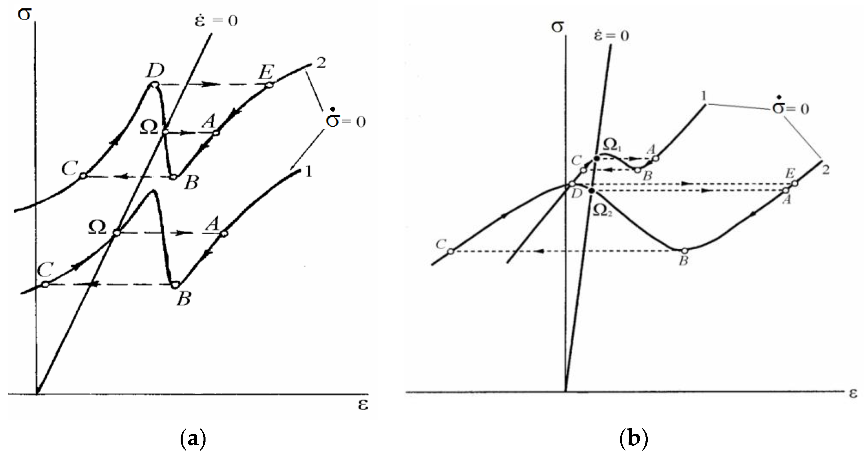
To analyze qualitatively Equations (13) and (14), we take advantage of the isocline method by equating to zero the left sides of the equations. Then

$$\sigma =\frac{\eta }{{\theta }_{\sigma }}\epsilon =G\epsilon$$

(15)

and

$$\sigma =\frac{{\sigma }_0+{\sigma }_y}{1-\left({\theta }_{\sigma }/{\theta }_{\epsilon }\right)\epsilon }.$$

(16)

The 0-isoclines so obtained are shown in Figure 5a. Their analysis consists of the search of special points (points of intersection of 0-isoclines). The N-shaped form and the position of function (16) are determined by constants entering into it and by the strain ε. For small stresses, after achievement of the special point Ω, any small deviation from the equilibrium leads to the jump-like transition Ω → А to the stable isocline branch $\dot{\sigma }=0$. At low stresses, the point makes the cycle А → B → С → Ω, and the system returns to the equilibrium again. At high stresses (the upper curve), after disruption of the equilibrium Ω → А, the depicting point no longer returns to the equilibrium position and moves along the closed trajectory А → B → С → D → E → B. The first case corresponds to the propagation of the switching autowave (the Lüders front). The repetition of cycles in the second case indicates the formation of the phase autowave.

The function $f\left(\epsilon \right)$ can also be defined in another way. For example, for the thermal activation character of the relaxation process, this dependence can be logarithmic in character, which follows from the kinetics of the thermally activated plastic deformation [64]. Then

$$f\left(\epsilon \right)=\frac{A}{{\theta }_{\sigma }}\ln \epsilon +\frac{\sigma -{\sigma }_{\vartheta }}{{\theta }_{\sigma }},$$

(17)

where the constant A is determined by the mechanism of plastic strain and ${\sigma }_{\vartheta }$ is the stress function. The equation for the 0-isocline in this case has the form

$$\sigma ={\sigma }_{\vartheta }+A\ln \epsilon$$

(18)

shown in Figure 5b. The subsequent analysis also demonstrates the change in plastic flow modes. At low stresses (curve 1), the depicting point on the path Ω₁ → A → B → C returns to the equilibrium position. At high stresses (curve 2), the depicting point after transition Ω₂ → A moves along the trajectory B → C → D → E → B that corresponds to the formation of the phase autowave.

Thus, Equations (7), (8), (10), and (12) are applicable for a description of the formation of autowaves. With their help, the existence of switching and phase localized plasticity autowaves at stages of the yield plateau and linear work hardening, respectively, can be explained.

3.3. On the Application of the Autowave Representations

In physics of lattice defects, one of the first attempts to use Equation (7) belongs to Donth [65,66] who explained with its help the contribution of dislocation kink motion to the amplitude-dependent internal friction. Later on, such ideas were used directly to describe the self-organization of dislocation ensembles during plastic deformation. For example, the situation with propagation of strain fronts was studied in [67,68], where correct estimation was obtained of the autowave propagation velocity of inhomogeneous plastic shear (the switching autowave) for motion of the Lüders band.

In [69,70,71,72], the autowave representations were used to solve the problem of the jump-like strain and to analyze the formation of slip bands. For these purposes, the authors wrote dynamic equations for dislocation ensembles and considered conditions of forming slip bands from originally chaotic defect distribution. The complex structure of the strain waves propagating in the deforming medium and consisting of the head part of soliton type and of the oscillating tail gradually lagging behind the head part during motion was predicted. This effect can be considered as one of the mechanisms of autowave generation in deforming media. General analysis of the problem of stability of a dislocation ensemble demonstrated that dislocation density fluctuations lead to the emergence of stress concentrators in a deforming medium.

Apparently, the mechanisms of self-organization and formation of dislocation ensembles were considered most consistent and rigorously in [73,74,75,76]. Thus, in [74] the relationship between the strength and plasticity was analyzed on the examples of work hardening curves for some metals and alloys with the Face Centered Cube (FCC) lattice. The analysis was based on the criterion for the neck formation in a sample in tension and on the work hardening curve illustrating the dynamics of dislocation density in the material with increasing strain degree and the influence of structural factors of these processes.

The influence of the Peierls stress on the strength and strain before the neck formation was studied in [75] for metals and alloys in tension. The analysis was based on the equation of dynamics of dislocation density with strain determining the character of work hardening of the material and the influence of the Peierls stress on the parameters of this equation in terms of the annihilation coefficient of screw dislocations. In [76] the mechanism of work hardening and formation of fragmented dislocation structures in metals subject to severe plastic deformation was discussed based on the equations of dislocation kinetics.

The authors of [77,78], based on the autowave approach, succeeded in explaining the transition of the autowave strain modes to the plastic flow from the Lüders front to the phase autowave and the quadratic dependence of the autowave dispersion at the stage of linear work hardening. The authors of [79,80] considered, in detail, the possibility of self-organization of dislocation structures by a plastic flow, substantiated the introduction of the hydrodynamic strain flow component, and illustrated how such process affects the work hardening kinetics and dynamics. They demonstrated that the dynamics of the deformation processes obeys the laws of synergetics.

3.4. Generation of Plastic Strain Autowaves. Autowave Model

The mechanisms of influence of the values $\epsilon$ and $\sigma$ governing the plastic flow can be the following. The autocatalytic factor (strain) acts so that each accomplished shear initiates the similar process in the neighboring volume required for accommodation, so that the effective radius of action for this parameter is on the order of the shear zone size l, and its propagation velocity is commensurable with the dislocation velocity $V_{disl}$. The elastic energy liberated during each shear is redistributed within the volume, causing relative growth of the stress concentration, which impeds (damps) the plastic strain. The radius of action of this factor is commensurable with the sample size L>> l, and the propagation velocity is equal to that of the elastic waves $V_t>>V_{disl}.$ Such relationship between the action radii and the propagation rates of the activating and inhibiting factors that governs the process is necessary for autowave generation [34].

3.5. Plastic Strain as Self-Organization Process in a Medium

Haken [12] stated that “the system is called self-organizing if it acquires any spatial, time, or functional structure without specific external impact.” In this case, the localization dynamics, that is, spontaneous stratification of the medium into deforming and non-deforming volumes is equivalent to its self-orga­ni­zation, that is, ordering (structurization). An explanation of such processes is a traditional problem for synergetics.

Olemskoi [11,81,82,83] applied synergetic apparatus to a detailed description of problems of condensed state physics. In particular, he first succeeded in consideration from these positions the patterns of formation of single defects and localization autowaves in the plastic flow under active loading.

In [84,85,86,87,88,89,90,91], problems of structurization of condensed media were analyzed; in particular, the formation of localized plasticity autowaves and the nature of hydrodynamic and diffusion-like plastic flow modes. The application of these ideas directly to a solution of the plasticity problem signaled a new view on the plastic strain as on the process of self-organization of defective structure on different scale levels. Balankin [84,85] successfully used the synergetic approach to describe the strain nature and the destruction processes based on excitation mechanisms of the crystal lattice. In [86,87,88,89,90,91] the authors described the process of plastic strain as a nonequilibrium kinetic transition leading to plastic flow localization. Within the framework of this approach, the deforming material was considered as a system capable of generating dissipative structures more efficient in comparison with motion of single dislocations, in particular, plastic flow autowaves. This is in agreement with the results of investigations of dislocation structures in a plastic flow. Thus, for example, the authors of [92] established regularities of generation of new dislocation substructures during deformation and showed that a new structure emerges against the background of the old structure and is accompanied by its degradation. It is important that emergence of new substructures corresponds to a change in the mechanism of work hardening.

3.6. Structure of the Autowave Plastic Flow Model

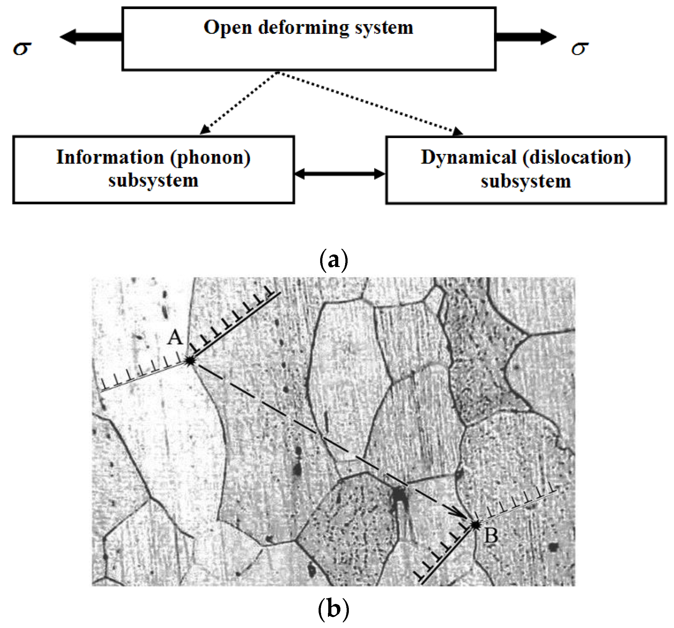
The new approach required the development of a self-organization model focused on the problem of plasticity of solids. It is conformed to the idea of Kadomtsev [45] who considered that “during self-organization of complex open physical systems, trends may emerge toward their stratification into information and dynamic subsystems”.

This claim is in agreement with representations about competition between the autocatalytic and damping factors discussed above, and a relationship can be seen of the dynamic and information subsystems with them. Therefore, to develop a model, we define the specificity of the information and dynamic subsystems in a deforming medium bearing in mind that

- The structure of the information and dynamic subsystems should be closely related to the processes that control the plastic flow,

- There should be a mechanism of subsystem interaction of such power that events in one subsystem could cause responses in another.

Deformation involves the elastic and plastic components. The elastic state at nominal (average) stresses ${\sigma }_{nom}<{\sigma }_y$ is characterized by the presence in the material of a set of dwelling stress concentrators with amplitude ${\sigma }_c>>{\sigma }_{nom}$ randomly distributed over the volume, which is typical of an active medium. For ${\sigma }_{nom}>{\sigma }_y$, the medium is transformed into the plastic state in which a part of the concentrators remains in the waiting state, and another part relaxes. This is taken into account in the Two-component plasticity model whose flowchart is shown in Figure 6a. In this case, the dynamic subsystem is formed by a set of relaxing concentrators—elementary plastic strain relaxation events, where thermally activated relaxation (destruction) of the concentrator is considered as an elementary plastic flow event of dislocation shear, twinning, etc. The information subsystem includes a set of elastic pulses of acoustic emission generated during relaxation events.

The state of a deforming medium in this model is characterized by wandering of acoustic pulses in the system of elastic stress concentrators. Being superimposed on the elastic concentrator fields, they increase the probability of plastic strain relaxation events. Autowave modes are generated due to interaction of the dynamic and information subsystems provided on the one hand, by generation of pulses of acoustic emission in each relaxation event, and on the other hand, by their absorption by dwelling concentrators. Thus, either spontaneous or induced relaxation is observed in the system by the condition ${\sigma }_{nom}>{\sigma }_y$; the latter is caused by activation of dwelling concentrators by acoustic emission pulses [93,94,95].

The scenario of plastic flow, as it is shown in Figure 6b, includes the two steps. First of all, transformations in the dynamic subsystem, that is, spontaneous or induced plastic shear (transformation of the waiting concentrator into the relaxing one and again into the dwelling one; points A and B). After that, transformations in the information subsystem, that is, emission of acoustic pulse in the process of concentrator destruction (point A) and its absorption by another dwelling concentrator (point C). Then these steps are repeated.

Thus, two effects, typically studied separately, are combined in the two-component model. The first effect is the acoustic emission accompanying the plastic flow events and conventionally used to non-destructive testing the material state [93,96]. The second effect is acoustic aided plasticity whose mechanism, explained in [94,95], consists of plasticization of the material by imposing stresses oscillating with ultrasonic frequency on a deforming object.

Obviously, the above-described mechanism is possible because of the known property of a nonlinear deforming medium to generate harmonics during elastic signal propagation. In this case, the elements of the medium can be related with these harmonics [45]. Thus, in particular, if the acoustic signal containing the harmonic of a certain frequency is generated in the process of destruction of the stress concentrator A, such harmonic can be absorbed by the accepting concentrator C of similar structure and spectrum with the corresponding increase of the impact.

3.7. Quantitative Estimations of Possibilities of the Model

Let us compare the expectation times for thermally activated relaxation events [64] in the absence of acoustic pulse (spontaneous relaxation)

$${\vartheta }_{sp}\approx {\omega }_D^{-1}\exp \left(\frac{U_0-\gamma \sigma }{k_{B}T}\right),$$

(19)

and after its imposition (induced relaxation)

$${\vartheta }_{ind}\approx {\omega }_D^{-1}\exp \left[\frac{U_0-\gamma \sigma -\delta U_{ac}}{k_{B}T}\right]\approx {\omega }_D^{-1}\exp \left[\frac{U_0-\gamma \left(\sigma +{\epsilon }_{ac}E\right)}{k_{B}T}\right].$$

(20)

In these equations, ${\omega }_D$ is the Debye frequency, $U_0$ is the potential barrier to be overcome during the relaxation event, $\gamma \approx b^{2}l\approx {10}^4{b}^3$ is the activation volume of this event [64], l is the size of the shear zone, $k_B$ is the Boltzmann constant, Т is temperature, and Е is the elastic modulus. With the help of calculations by Equations (19) and (20) we set the activation enthalpy of the destruction process as $U_0-\gamma \sigma \approx$ 0.5 eV [64], and the acoustic pulse with elastic strain amplitude ${\epsilon }_{ac}$ decreases this parameter by $\delta U\approx \gamma {\epsilon }_{ac}E\approx$ 0.1 eV. Calculation for $k_{B}T\approx$ 1/40 eV yields ${\vartheta }_{sp}\approx$ 5 × 10⁻⁵ s and ${\vartheta }_{ind}\approx$ 9 × 10^–7 s $<<{\vartheta }_{sp}.$ Such estimations explain the principal possibility of plastic flow acceleration under the action of acoustic pulses and confirm the correctness of the model.

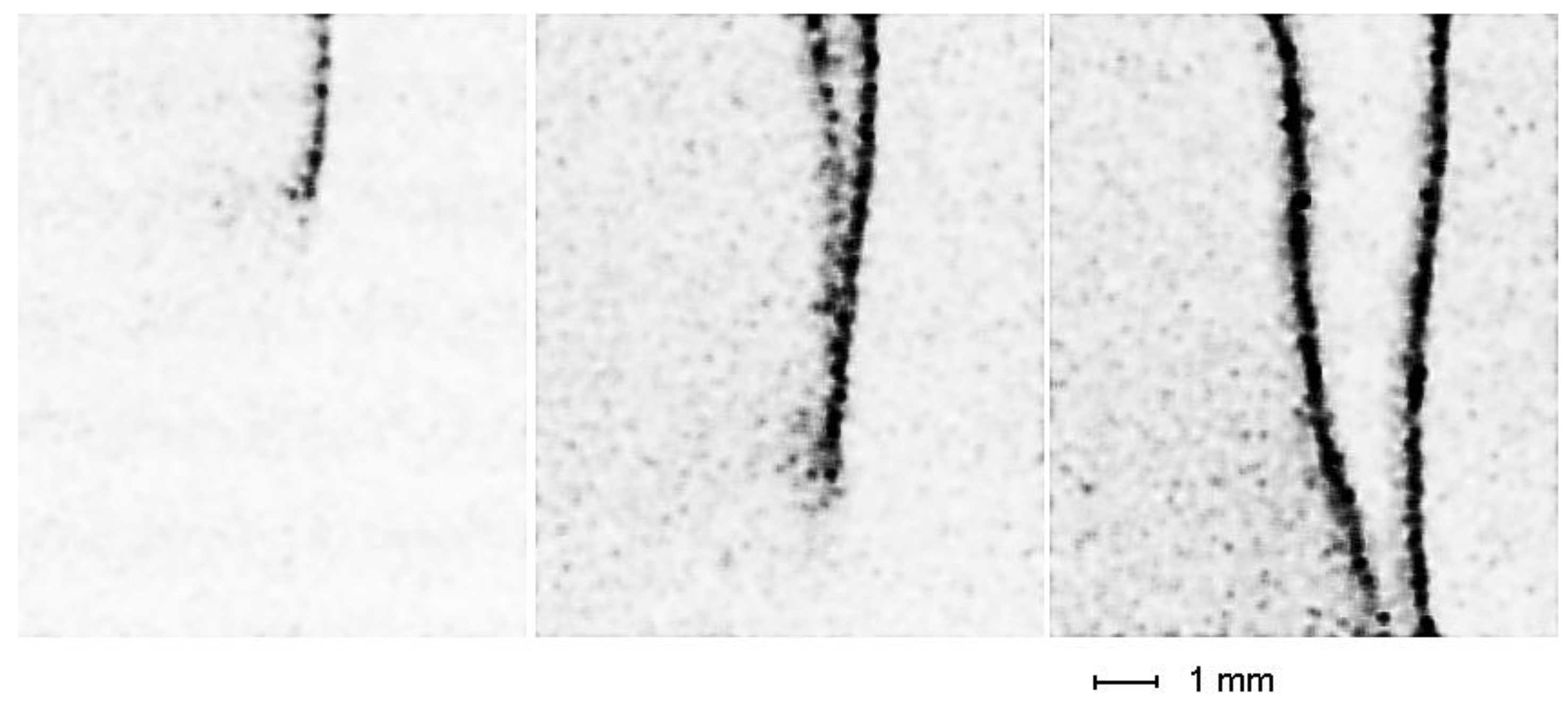
Equations (19) and (20) demonstrate the possibility of induced destruction of stress concentrators. It seems likely that the rate of localized plasticity autowave dynamics is determined by the time of plasticity nucleus growth from a nucleus that can be identified with the intergrowth of the Lüders band through the sample (${\tau }_L\approx 10\mathrm{s}>>{\vartheta }_{sp}$, Figure 7).

The principal problem in explanation of the autowave nature irrespective of the system nature matches the macroscopic autowave scale with the microscale of internal interactions. In the context of the model being developed, it can be explained as follows. Let a shear emits a pulse of transverse acoustic waves with frequency ${\omega }_m\approx$ 10⁶ Hz corresponding to a maximum of the spectrum [93].

As shown in [97], having passed through an elastically stressed region, such pulse is split into two orthogonally polarized acoustic waves propagating with velocities $v_1$ and $v_2\ne v_1$. The difference between their wavelengths

$$\delta L=L_2-L_1\approx \frac{v_2-v_1}{{\omega }_m}\approx \frac{{\sigma }_2-{\sigma }_1}{2{\omega }_m{\rho }_0{V}_t}$$

(21)

reaches ~10^–4 m provided that the difference between the principal normal stresses ${\sigma }_2-{\sigma }_1\approx$ 10² MPa in Equation (21), the material density ${\rho }_0\approx$ 5 × 10³ kg/m³, and the sound velocity $V_t$ ≈ 10³ m/s. The probability of activation of a new shear increases when the maxima of ${\sigma }^2$ coincide in both waves, that is, when the elastic energy is maximal. This corresponds to the condition $L^2/\delta L\approx \lambda \approx$ 10^–2 m, which is close to the observable autowave length and explains the origin of the plasticity nuclei at the distance ~λ from the existing strain front at the expense of the process of acoustic initiation of strain.

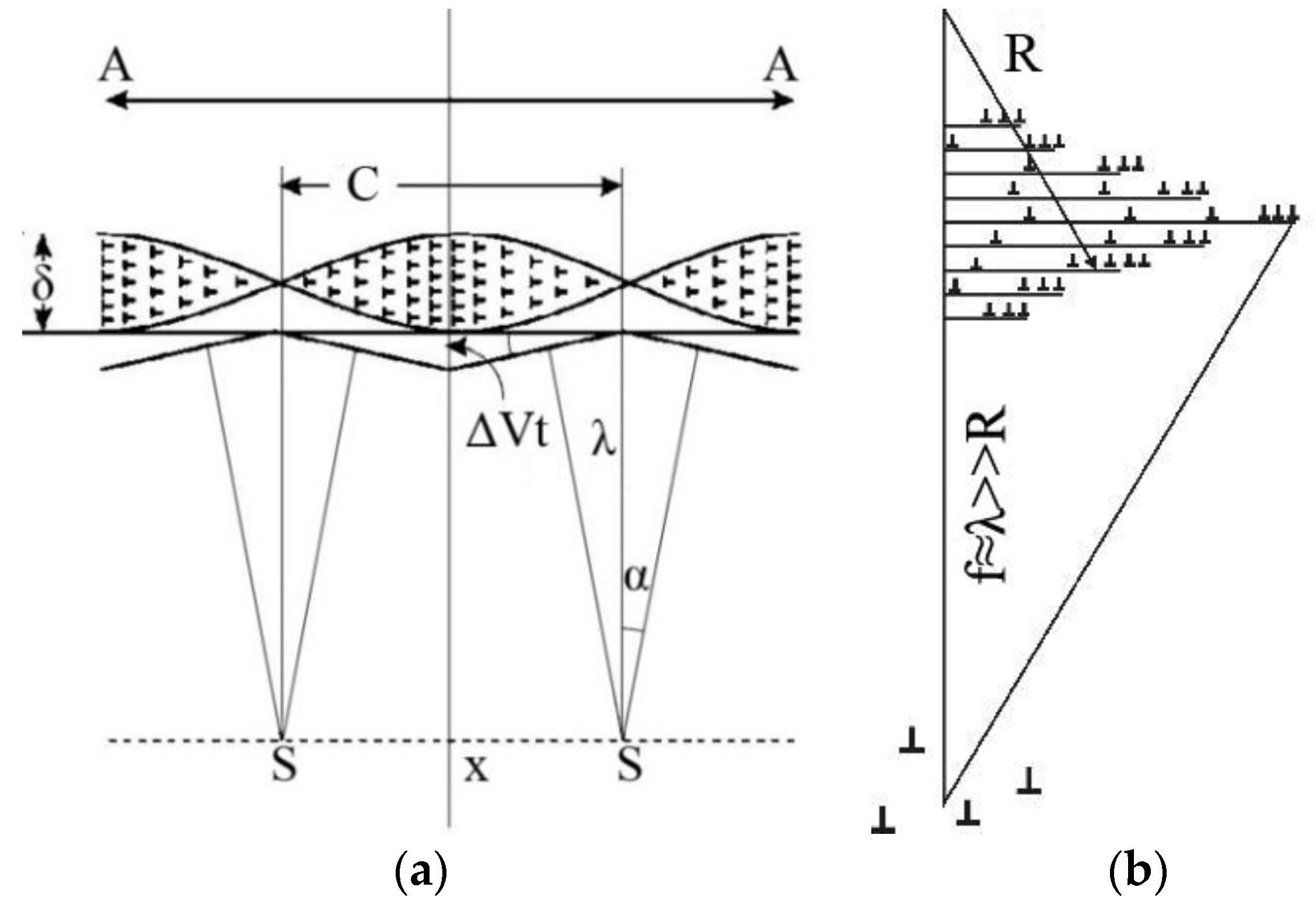
Another variant of estimation is based on an analysis of acoustic signal propagation through a fragment with inhomogeneous density of dislocations of the type of the existing plastic flow nucleus (Figure 8a). If the dislocation density in the fragment decreases from the nucleus toward the periphery, the internal stresses ${\sigma }_i\approx Gb{\rho }_d^{1/2}$ [6] are inhomogeneously distributed. Such fragment can be considered as an acoustic lens with diameter C. Together with the dependence $V_t~{\sigma }_i$ [60], this causes rotation of the plane wave front А–А passing in this region through a small angle α.

The waves from neighboring regions playing the role of lenses are focused onto the symmetry axis where the level of the elastic stress increases, thereby increasing the probability of relaxation plasticity events.

This initiates the formation of a new strain nucleus at the same distance ~λ from the initial. Simple geometric calculation the details of which and the designations are explained in Figure 8a demonstrates that

$$\lambda \approx \frac{C}{2\sin \alpha }\approx \frac{C}{2\tan \alpha }\approx \frac{1}{\Delta V_t\delta /C{V}_t}\approx C\cdot \frac{C}{2\delta }\cdot \frac{V_t}{\Delta V_t}.$$

(22)

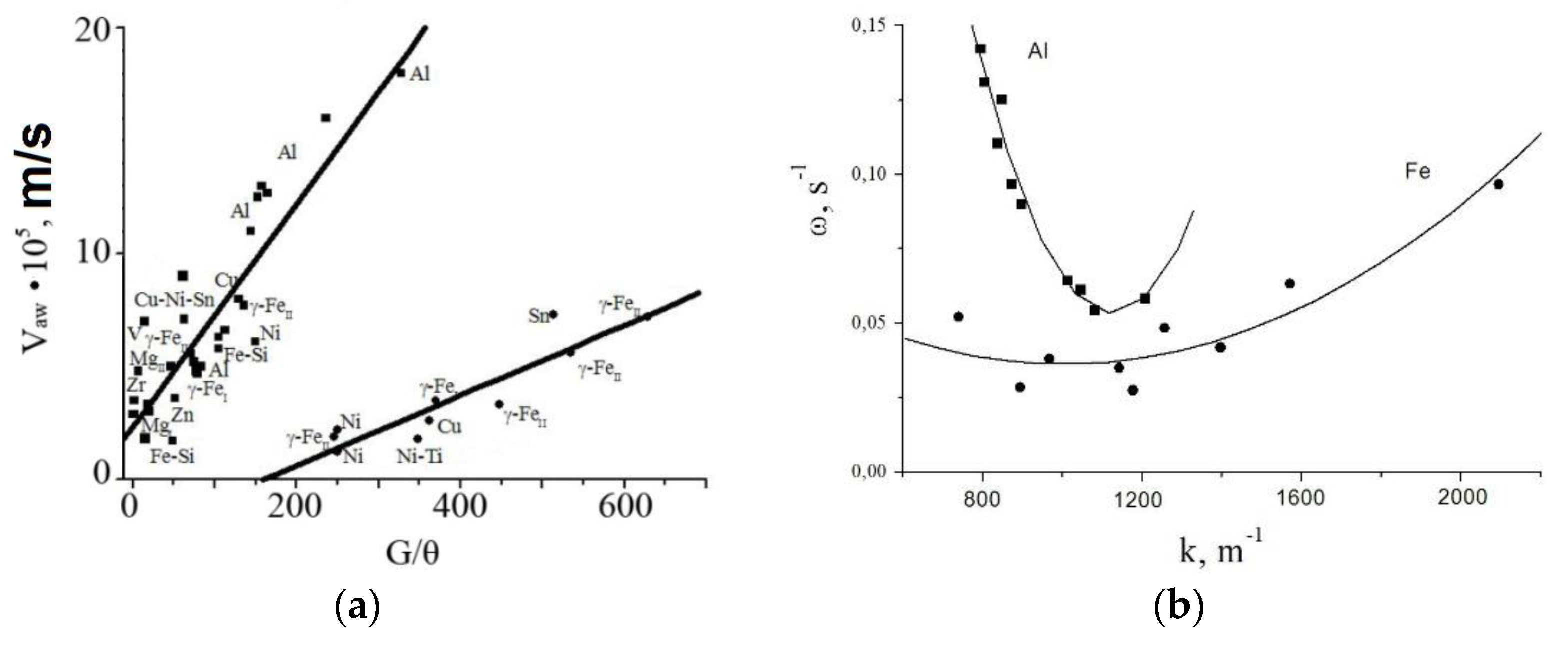
It is convenient to estimate the effect quantitatively for polycrystalline Al in which the velocity is $V_t\approx$ 3⋅10³ m/s, and its experimentally determined range of variation in the plastic strain interval corresponding to the stage of parabolic hardening is $\Delta V_t\le$10 m/s [43]. For the fragment size δ ≈ 10^–7 m and the ratio $C/2\delta \approx$ 10, we obtain λ ≈ 10^–2 m, which is close to the observable distance between the localized strain nuclei (autowave strain length). Since $\lambda >>C>b$, we can consider that Equation (22) relates the microscale of the dislocation substructures and the macroscale of the autowave deformation.

A simpler variant of such estimation is possible. Since the velocity of elastic waves depends on the strain and the dislocations are conventionally distributed inhomogeneously. The inhomogeneity zone with size $l_d$ can be considered as an acoustic lens with curvature radius $R\approx l{}_d$. Its focal length $\xi$ (Figure 8b) is [49]

$$\xi =\frac{R}{\kappa -1},$$

(23)

where $\kappa =V_0/V$ is the refractive index of sound waves in the deforming medium. From experimental data presented in [60], it follows that $\kappa \le$1.002 almost until destruction; during deformation of Al, $R\approx l{}_d$ ≈ 10^–5 m. Then according to Equation (23) $\xi \approx \lambda \approx$ 5 × 10^–3 m. The probability of stress concentrator destruction increases at this distance, and a new strain localization nucleus is formed. Since the parameters $\kappa$ and R are determined by the material structure, the dynamics of the strain nuclei in the plastic flow can control reorganization of the autowave strain localization pattern. Dislocation ensembles with inhomogeneous distribution of defects in the volume—dislocation fragments, cells etc.—can play the role of acoustic lenses [4,7,98].

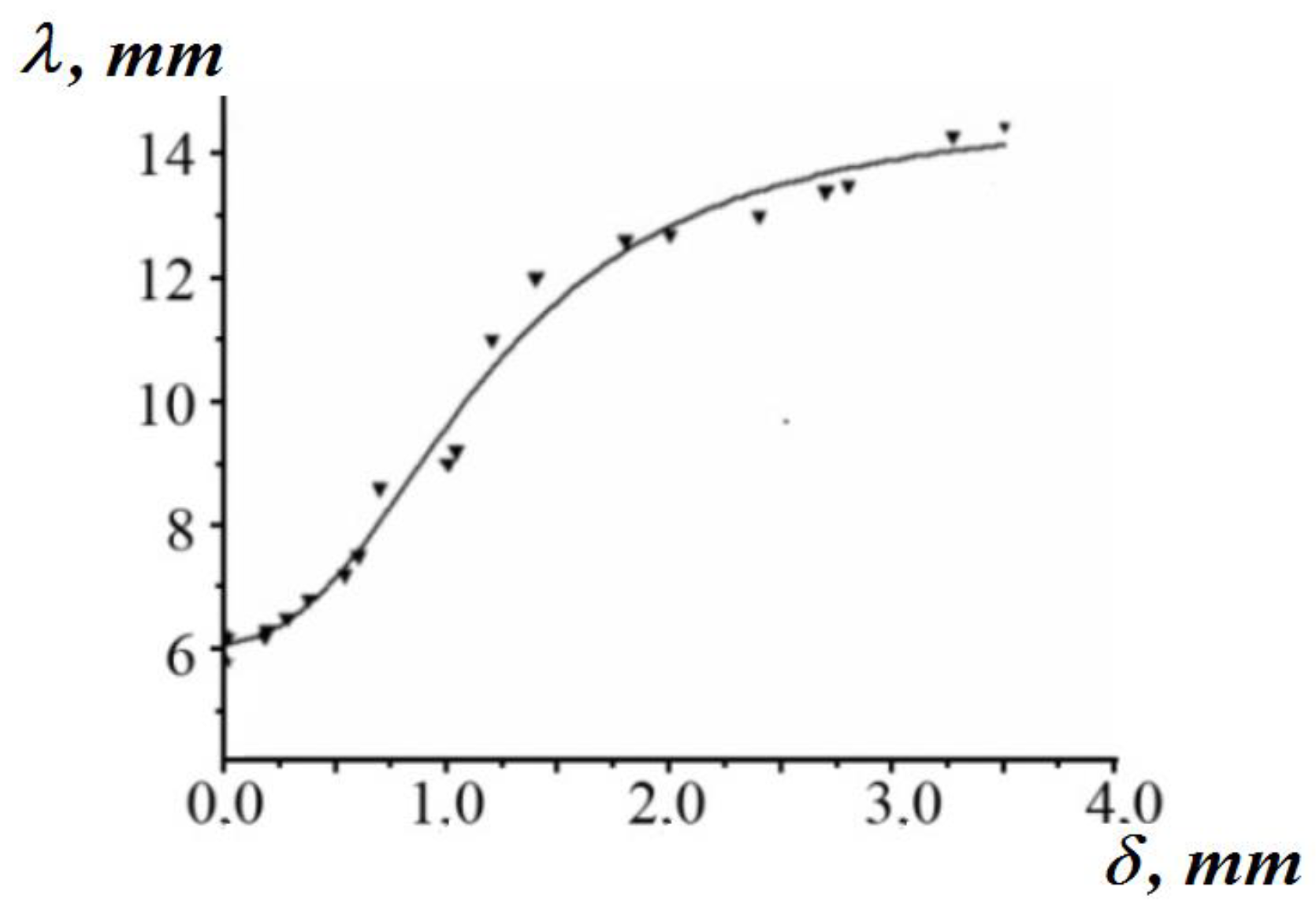
In these cases, variants of propagation and behavior of macroscopic localized strain zones can be caused by the change of the acoustic lens geometry (parameters C and δ and their ratio $C/2\delta$) or dislocation distributions during plastic flow. According to Equation (22), the increase of the fragment size initiates growth of λ and can cause motion of the plastic flow nucleus along the tension axis at the stage of linear work hardening.

The above estimations show that the most complicated problem of plastic flow physics, which is the emergence of macroscopic autowave scale of ~10^–2 m in actual deforming material whose structural defects (dislocations) possess much smaller spatial scale on the order of the Bürgers vector of ~10^–10 m, finds a non-contradictory explanation in the context of the proposed two-component model of localized plastic flow dynamics.

4. Elastic-Plastic Strain Invariant

The interaction of elastic waves with plastic shears directly plays the principal role in the two-component model of localized plasticity. For this reason, the existence of the quantitative relationship between the corresponding characteristics was established with the help of numerical analysis of quantitative data of the localized plastic flow dynamics.

4.1. On the Existence of the Elastic-Plastic Invariant

For phase localized plasticity autowaves, the relationship

$$\frac{\lambda V_{aw}}{\chi V_t}\approx const$$

(24)

or $\lambda V_{aw}~\chi V_t$ holds true, where $\lambda$ and $V_{aw}$ have been determined above, $\chi$ is the interplanar distance corresponding to the maximum intensity of the X-ray reflection, and $V_t$ is the propagation rate of transverse ultrasonic waves. The last two parameters for the materials are determined in [99,100]. To elucidate the meaning of Equation (24), data on the value of the ratio $\lambda V_{aw}/\chi V_t$ obtained for different strain modes of the investigated materials and presented in

Table 1. The comparison of $\chi V_t$ and $\lambda V_{aw}$ products for metals.

×107 m2/s	Linear Work Hardening Stage
	Cu	Zn	Al	Zr	Ti	V	Nb	α-Fe	γ-Fe	Ni	Co	Mo
$\lambda V_{aw}$	3.6	3.7	7.9	3.7	2.5	2.8	1.8	2.55	2.2	2.1	3.0	1.2
$\chi V_t$	4.8	11.9	7.5	11.9	7.9	6.2	5.3	4.7	6.5	6.0	6.0	7.4
$\lambda V_{aw}/\chi V_t$	0.75	0.3	1.1	0.3	0.3	0.45	0.33	0.54	0.34	0.35	0.5	0.2

,

Table 2. The comparison of $\chi V_t$ and $\lambda V_{aw}$ products for alkali-halide crystals and rocks.

×107 m2/s	KCl	NaCl	LiF	Marble	Sandstone
$\lambda V_{aw}$	3.0	3.1	4.3	1.75	0.6
$\chi V_t$	7.0	7.5	8.8	3.7	1.5
$\lambda V_{aw}/\chi V_t$	0.43	0.4	0.5	0.5	0.4

and

Table 3. The comparison of $\chi V_t$ and $\lambda V_{aw}$ products for individual dislocation paths.

×107 m2/s	NaCl	LiF	CsI	KCl	Zn
$l{V}_{disl}$	4.1	4.1	1.9	4.1	1.8
$\chi V_t$	7.3	8.6	4.0	6.8	4.0
$l{V}_{disl}/\chi V_t$	0.56	0.47	0.47	0.6	0.45

were statistically analyzed in [47] for the following cases:

- Linear work hardening and easy glide in single crystals and polycrystals,

- Compression strain of alkali-halide crystals (KCl, NaCl, and LiF),

- Compression strain of rocks (marble and sandstone),

- Creep of polycrystalline aluminum,

- Strain caused by motion of individual dislocations in Zn, CsI, NaCl, KCl, and LiF single crystals [101,102]; here the free path of dislocations was used instead of the autowave length.

Investigations were performed for single crystals and polycrystals deformed by slipping, twinning (γ-Fe and marble), and grain boundary processes (sandstone). On diagrams $\sigma \left(\epsilon \right)$ for the investigated materials, sections of linear strain hardening can be seen in which the phase localized plastic flow autowaves emerge. The ratios $\lambda V_{aw}/\chi V_t$ used to estimate the data are given in Table 1, Table 2 and Table 3 for 38 investigated materials. As follows from these Tables, $0.2\le \widehat{Z}\le 1.1.$

To elucidate the nature of the invariant, the question about the law of $\widehat{Z}$ distribution in a sample is of principal importance. To answer it, as a 0-hypothesis it was accepted that sizes $\widehat{Z}$ obey a normal law [47]. This means that the correlation of their behavior in experimentally established limits with the behavior of any characteristic of the material is absent.

To test the 0-hypothesis by the graphic method, data of Table 1, Table 2 and Table 3 were transformed into the variation series ${\widehat{Z}}_1<{\widehat{Z}}_2<{\widehat{Z}}_3<\dots <{\widehat{Z}}_i<\dots <{\widehat{Z}}_{n-1}<{\widehat{Z}}_{n=38}$ whose terms serve as arguments for the search of numerical values of quintiles $-\infty <Q<\infty$ of the normal distribution corresponding to $i/\left(n+1\right)$ [47]. The hypothesis about the normal distributions of $\widehat{Z}$ is accepted, if Q is actually linear in $\widehat{Z}.$ As can be seen from Figure 9, the dependence $Q\left(\widehat{Z}\right)$ in the coordinates $Q-\widehat{Z}$ is linear in character. Thus, the parameter $\widehat{Z}$ obeys the normal distribution, and variations of $\widehat{Z}$ for $0.2\le \widehat{Z}\le 1.1$ depend only on experimental errors in measuring the parameters of the phase localized plasticity autowaves.

Thus, the average value $\langle \lambda V_{aw}/\chi V_t\rangle$, its variance ${\sigma }^2$, and standard error $\pm \sqrt{{\sigma }^2/n}$ [47] were determined. It turned out that

$${\langle \frac{\lambda V_{aw}}{\chi V_t}\rangle }_{n=38}=\langle \widehat{Z}\rangle =0.49\pm 0.04\approx \frac{1}{2}.$$

(25)

Since $\left|\sqrt{{\sigma }^2/n}\right|<<\widehat{Z},$ it is possible to suppose that, the value $\widehat{Z}$ is evaluated sufficiently exactly.

Equation (25), called the Elastic-plastic strain invariant, quantitatively relates the characteristics of the elastic waves (χ and $V_t$) to the characteristics of plastic flow localization autowaves ($\lambda$ and $V_{aw}$), combining the elastic (${\epsilon }_{el}<<1$) and plastic (${\epsilon }_{pl}\approx 1$) strain components simultaneously acting in a solid. In this case, the product $\chi V_t$ describes the kinetics of redistributions of elastic stresses with the velocity $V_t$, and the product $\lambda V_{aw}$ plays the same role for reorganization of the localized plastic flow patterns with the velocity $V_{aw}$.

Thus, the elastic-plastic strain invariant acquires the status of the characteristic suitable for a description of plastic flow processes in materials irrespective of their nature and operating plasticity micromechanisms. To refine its physical meaning, we take into account that $V_t\approx \chi \cdot \left({\omega }_D/2\pi \right)$ and $\hslash {\omega }_D\approx k_B{\theta }_D$, where $\hslash =h/2\pi$ is the Planck constant and ${\theta }_D$ is the Debye parameter [103]. Then using these substitutions, we have

$$\lambda V_{aw}=\widehat{Z}\chi V_t\approx \widehat{Z}{\chi }^2\frac{{\omega }_D}{2\pi }\approx \widehat{Z}\cdot \frac{k_B}{h}\cdot \left({\chi }^2{\theta }_D\right).$$

(26)

The parameter $\lambda V_{aw}$ that characterizes the plastic flow at the stage of linear strain hardening (the plasticity parameter) can be predicted directly from Equation (26) for the known values $\chi$ and ${\theta }_D$. The results of such calculations, presented in

Table 4. The estimation of $\lambda V_{aw}$ values via lattice characteristics of metals.

Metal	χ	θD	${(\mathit{\lambda }{\mathit{V}}_{\mathit{a}\mathit{w}})}^{\left(\mathbf{calc}\right)}$	${(\mathit{\lambda }{\mathit{V}}_{\mathit{a}\mathit{w}})}^{\left(\mathbf{exp}\right)}$	${{\left(\mathit{\lambda }{\mathit{V}}_{\mathit{a}\mathit{w}}\right)}^{\left(\mathbf{calc}\right)}/\left(\mathit{\lambda }{\mathit{V}}_{\mathit{a}\mathit{w}}\right)}^{\left(\mathbf{exp}\right)}$
	×1010 m	K	×107 m2/s	×107 m2/s
Ni	2.03	375	1.6	2.1	0.8
Cu	2.08	315	1.4	3.6	0.4
Al	2.33	394	2.2	2.6	0.8
Mo	2.22	380	1.9	1.2	1.6
Co	2.18	385	1.9	1.3	1.5
Sn	3.75	170	2.5	2.4	1.0
α-Fe	2.02	420	1.8	2.55	0.7
In	2.72	129	0.95	2.6	0.4
Zn	2.077	234	1.0	3.7	0.3
Cd	2.34	120	0.65	0.9	0.7
Mg	2.45	318	1.9	9.9	0.2

, show that Equation (26) correctly predicts the order of magnitude of $\lambda V_{aw}$. Since the Debye parameter depends on the temperature [103], Equation (26) can be used for prediction of the temperature dependence of the plasticity parameter $\lambda V_{aw}$.

4.2. Nature of the Elastic-Plastic Strain Invariant

Relating the characteristics of the elastic ($\chi$ and $V_t$) and plastic ($\lambda$ and $V_{aw}$) deformation components, invariant (25) plays an important role for a description of dynamics of the localized plasticity. We now look at some details of its nature. As shown above, the plastic strain localization is a consequence of self-organization of a nonlinear active deforming medium. As is well known, the common feature of the self-organization processes in open systems such as a deforming body is a decrease in the entropy [16]. This condition is indeed satisfied in the process of generation of localized plastic flow autowaves [104], and the use of the entropy to explain the invariant nature is well justified.

The two-component plasticity model is based on the emergence and destruction (relaxation) of elastic stress concentrators accompanied by generation of dislocations. This means that during deformation, the spatiotemporal distributions of the stress fields $\sigma \left(x,y,t\right)$ and plastic strains $\epsilon \left(x,y,t\right)$ undergo interrelated transformations. The velocities $V_t$ and $V_{aw}$ control the transformation kinetics of the elastic and plastic fields, and the lengths $\chi$ and $\lambda$ are the spatial scales of these processes. For this reason, it is convenient to write invariant (25) in the form

$$\frac{\lambda \cdot V_{aw}}{\chi \cdot V_t}=\frac{\lambda }{\chi }\cdot \frac{V_{aw}}{V_t}=\frac{\lambda /\chi }{V_t/V_{aw}}=\widehat{Z}<1,$$

(27)

where the ratios $\lambda /\chi =p_{scale}>1$ and $V_t/V_{aw}=p_{kin}>1$ make sense of the scale and kinetic thermodynamic probabilities [105]. The scale thermodynamic probability $p_{scale}$ is interpreted as the number of possible nuclei of emergence of the localized plastic flow autowaves in a deforming medium, that is, it is determined by significant difference between the spatial scales of elastic and plastic deformation processes. The structure parameter $p_{scale}$ is dissipative one and causes the autowave dispersion, that is, destroys the order. As to the kinetic thermodynamic probability $p_{kin}$, it determines the choice by a deforming system of the observable autowave velocity from the range of its possible values $0\le V_{aw}\le V_t$. This parameter, on the contrary, promotes ordering, because it can be associated with the rule of subordination of slow processes to the fast one’s characteristic for synergetics [12].

In this case, from Equation (27) it follows that

$$\ln \widehat{Z}=\ln p_{scale}-\ln p_{kin}$$

(28)

that corresponds to equations for changes in the entropy due to different scales

$$\Delta S_{scale}=k_B\ln \frac{\lambda }{\chi }=k_B\ln p_{scale},$$

(29)

and different velocities

$$\Delta S_{kin}=k_B\ln \frac{V_t}{V_{aw}}=k_B\ln p_{kin}.$$

(30)

From Equations (28)–(30) we finally obtain

$$\Delta S=-k_B\ln p_{kin}+k_B\ln p_{scale}=-\Delta S_{kin}+S_{scale}=k_B\ln \frac{1}{2}<0,$$

(31)

from which it follows that the entropy of the deforming system decreases during phase autowave generation. The signs of $\Delta S_{scale}>0$ and $\Delta S_{kin}<0$ in Equation (31) confirm the antagonism of contributions of the scale and kinetic factors to the nature of the localized plasticity.

The parameter $\Delta S<0$ characterizes the decrease in the entropy due to generation of the phase autowave of a localized flow characteristic for the self-organization processes in a deforming medium. Since

$$\widehat{Z}=\exp \left(\Delta S/k_B\right)\approx \frac{1}{2},$$

(32)

then $\Delta S=k_B\mathrm{l}\mathrm{n}1/2\approx -0,7k_B$ per elementary relaxation event [106].

Let us elucidate the nature of Equations (7) and (8) considering the relationship between the elastic and plastic displacements of elements of the medium at small deviations from the equilibrium. In this case, the displacement velocities during transformations of the strain and stress fields are linear in gradients of plastic and elastic strains to within the first order of smallness [105] so that

$${\dot{u}}_{pl}^{\left(p\right)}\approx D_{\epsilon \epsilon }\nabla {\epsilon }_{pl},$$

(33)

$${\dot{u}}_{el}^{\left(p\right)}\approx D_{\sigma \sigma }\nabla {\epsilon }_{el},$$

(34)

respectively. We also take into account the occurrence of velocities additional to Equations (33) and (34) due to strain–stress interactions

$${\dot{u}}_{el}^{\left(ad\right)}\approx D_{\epsilon \sigma }\nabla {\epsilon }_{pl},$$

(35)

$${\dot{u}}_{pl}^{\left(ad\right)}\approx D_{\sigma \epsilon }\nabla {\epsilon }_{el}.$$

(36)

Here it has been accepted that $\lambda V_{aw}\equiv D_{\epsilon \sigma }$ and $\chi V_t\equiv D_{\sigma \epsilon }$.

Now from Equations (33)–(36) follows

$$\{\begin{array}{}\mathrm{(37)}& {\dot{u}}_{pl}=D_{\epsilon \epsilon }\nabla \epsilon +D_{\epsilon \sigma }\nabla {\epsilon }_{el},\hfill \mathrm{(38)}& {\dot{u}}_{el}=D_{\sigma \epsilon }\nabla {\epsilon }_{el}+D_{\sigma \sigma }\nabla \epsilon .\hfill \end{array}$$

Their coefficients of these equations form the matrix $\left[\begin{array}{cc}{D}_{\epsilon \epsilon }& D_{\epsilon \sigma }\\ D_{\sigma \epsilon }& D_{\sigma \sigma }\end{array}\right]$ [105] that explains double subscripts of the coefficients D in Equations (7), (8), etc. According to the Onsager principle [105,107], the non-diagonal elements of this matrix are equal, that is, $\lambda V_{aw}\equiv D_{\epsilon \sigma }=D_{\sigma \epsilon }\equiv \chi V_t$. At the same time, the diagonal elements $D_{\epsilon \epsilon }$ and $D_{\sigma \sigma }$, which serve as the coefficients of autowave Equations (7) and (8), are not necessarily equal: below it will be shown that $D{}_{\epsilon \epsilon }<<D_{\sigma \sigma }.$

4.3. Invariant as the Master Equation of the Autowave Model of Plasticity

Since invariant (25) relates the characteristics of simultaneously proceeding elastic and plastic processes in a deforming medium, it plays a role of the Master equation of autowave mechanics of localized plastic flow being developed. This is confirmed by the circumstance that invariant (25) has a number of consequences that can be used not only to understand the nature of some important features of dynamics of localized plasticity, but also to describe them quantitatively. We consider these consequences below.

4.3.1. Velocity of the Localized Plasticity Autowaves

Differentiating Equation (25) with respect to the deformation ε

$$\lambda \frac{d{V}_{aw}}{d\epsilon }+V_{aw}\frac{d\lambda }{d\epsilon }=\widehat{Z}\cdot \chi \frac{d{V}_t}{d\epsilon }+\widehat{Z}\cdot V_t\frac{d\chi }{d\epsilon }$$

(39)

and writing the result for V_aw, we obtain

$$V_{aw}={\left(\frac{d\lambda }{d\epsilon }\right)}^{-1}\left(\widehat{Z}\cdot \chi \frac{d{V}_t}{d\epsilon }+\widehat{Z}\cdot V_t\frac{d\chi }{d\epsilon }-\lambda \frac{d{V}_{aw}}{d\epsilon }\right).$$

(40)

The interplanar distance χ is independent of the plastic strain, so that $\widehat{Z}\cdot V_t\cdot d\chi /d\epsilon =0$, and

$$V_{aw}=\widehat{Z}\chi \cdot \frac{d{V}_t}{d\lambda }-\lambda \cdot \frac{d{V}_{aw}}{d\lambda }.$$

(41)

Transformations of Equation (41) lead to the relationship

$$V_{aw}=\widehat{Z}\chi \cdot \frac{d{V}_t}{d\lambda }-\chi \cdot \frac{d{V}_{aw}}{d\lambda }\cdot \frac{\lambda }{\chi }\approx V_0+\frac{\mathsf{\Xi }}{\theta },$$

(42)

analogous to the experimentally obtained dependence $V_{aw}\left(\theta \right)~{\theta }^{-1}$ if we express the work hardening coefficient as the ratio of the structural parameters λ and $\chi <<\lambda$ [5], that is, as $\theta \approx \chi /\lambda$.

4.3.2. Dispersion of the Localized Plasticity Autowaves

Let us write down invariant (25) in the form

$$V_{aw}=\frac{\mathsf{\Theta }}{\lambda }=\frac{\mathsf{\Theta }}{2\pi }\cdot k$$

(43)

where $\mathsf{\Theta }=\widehat{Z}\chi V_t$. If $V_{aw}=d\omega /dk$, then $d\omega =\left(\mathsf{\Theta }/2\pi \right)\cdot k\cdot dk.$ In this case,

$${\displaystyle \underset{{\omega }_0}{\overset{\omega }{\int }}d\omega }=\frac{\mathsf{\Theta }}{2\pi }{\displaystyle \underset{0}{\overset{k-k_0}{\int }}k\cdot dk},$$

(44)

and the dispersion law for the localized plastic flow autowaves acquires the quadratic form

$$\omega \left(k\right)={\omega }_0+\frac{\mathsf{\Theta }}{4\pi }{\left(k-k_0\right)}^2,$$

(45)

where $\mathsf{\Theta }/4\pi \equiv \alpha$ is the parameter used in Equation (5).

In this case, the corresponding coefficients can also be estimated quantitatively. Writing Equation (26) in the form

$$V_{aw}\approx \widehat{Z}{\chi }^2\frac{k_B{\theta }_D}{h}\cdot \frac{1}{\lambda }\approx \widehat{Z}{\chi }^2\frac{k_B{\theta }_D}{h}\cdot k\approx \varsigma \cdot k$$

(46)

we can calculate the coefficient $\varsigma =\widehat{Z}{\chi }^2\cdot k_B{\theta }_D/h\approx \widehat{Z}{\chi }^2\cdot {\omega }_D$ for the parameters ${\chi }^{\left(\mathsf{\Phi }\mathsf{\epsilon }\right)}$, ${\chi }^{\left(\mathrm{A}\mathsf{\lambda }\right)}$, ${\theta }_D^{\left(\mathrm{Fe}\right)}=$ 420 K, and ${\theta }_D^{\left(Al\right)}=$ 394 K [103]. Then ${\varsigma }^{\left(Fe\right)}\approx$ 3.7 × 10^-7 m²/s and ${\varsigma }^{\left(Al\right)}\approx$4.45 × 10^–7 m²/s. This is in agreement with values ${\varsigma }^{\left(Fe\right)}=$ (1 ± 0.08) × 10^–7 m²/s and ${\varsigma }^{\left(Al\right)}=$ (12.9 ± 0.15) × 10^–7 m²/s experimentally determined from the dependence $V_{aw}\left(k\right)$ presented in [25].

4.3.3. The Material Structure and the Localized Plasticity Autowaves

It follows from invariant (25) that

$$\lambda =\widehat{Z}\chi \cdot \frac{V_t}{V_{aw}}.$$

(47)

If the velocities $V_t$ and $V_{aw}$ depend on the grain size $\delta$, then differentiation of Equation (47) with respect to $\delta$ yields

$$\frac{d\lambda }{d\delta }=\widehat{Z}\chi \cdot \frac{d}{d\delta }\left(\frac{V_t}{V_{aw}}\right)=\widehat{Z}\chi \cdot \left(\frac{V_{aw}\cdot d{V}_t/d\delta -V_t\cdot d{V}_{aw}/d\delta }{V_{aw}^2}\right),$$

(48)

from which it follows that

$$d\lambda =\widehat{Z}\chi \cdot \left(\frac{d{V}_t}{d\delta }\cdot \frac{1}{V_{aw}}-V_t\frac{d{V}_{aw}}{d\delta }\cdot \frac{1}{V_{aw}^2}\right)\cdot d\delta =\left(a_1\lambda -a_2{\lambda }^2\right)\cdot d\delta ,$$

(49)

where $a_1=\frac{1}{V_t}\cdot \frac{d{V}_t}{d\delta }=\frac{d\ln V_t}{d\delta }$ and $a_2=\frac{1}{\widehat{Z}\chi V_t}\cdot \frac{d{V}_{aw}}{d\delta }$ since $V_{aw}=\widehat{Z}\chi V_t\cdot \frac{1}{\lambda }.$ A solution of differential Equation (49) is Verhulst function

$$\lambda \left(\delta \right)={\lambda }_0+\frac{a_1/a_2}{1+C\exp (-a_1\delta )},$$

(50)

obtained experimentally for Al with grain sizes 5 × 10^–3 $\le \delta \le$ 15 mm. In Equation (50), ${\lambda }_0=const$ and C is the integration constant (see above).

4.3.4. Elastic-Plastic Invariant and the Hall–Petch Relationship

It is well known that the mechanical characteristics of polycrystalline materials (yield stress, strength limit, flow stress, and others) depend on such structural parameter, as the grain size [18,108]. The corresponding dependences are usually linear in the co-ordinates “property – ${\delta }^{-1/2}$”. It makes sense to check the validity of invariant (25) for two intervals of grain sizes $5\cdot {10}^{-6}\le \delta \le {10}^{-4}$ m and ${10}^{-4}\le \delta \le 5\cdot {10}^{-3}$ m. Results given in

Table 5. Elastic-plastic invariant for two grain size ranges.

Grain Size Ranges	$\mathit{\chi }{\mathit{V}}_{\mathit{t}}\cdot {10}^7$	$\mathit{\lambda }{\mathit{V}}_{\mathit{a}\mathit{w}}\cdot {10}^7$	$\frac{\mathit{\lambda }{\mathit{V}}_{\mathit{a}\mathit{w}}}{\mathit{\chi }{\mathit{V}}_{\mathit{t}}}$
m	m2/s
$5\cdot {10}^{-6}\le \delta \le {10}^{-4}$	5.13	2.61	~0.5
${10}^{-4}\le \delta \le 5\cdot {10}^{-3}$	6.17	3.12	~0.5

indicate the validity of the elastic-plastic invariant under these conditions.

4.3.5. Scale Effect for the Autowaves

If the autowave lengths are measured in samples of different lengths L, then

$$\frac{d}{dL}\left(\lambda V_{aw}\right)=\frac{d\lambda }{dL}{V}_{aw}+\lambda \frac{d{V}_{aw}}{dL}=\widehat{Z}\frac{d}{dL}\left(\chi V_t\right)=0$$

(51)

and

$$\frac{d\lambda }{dL}=-\frac{\lambda }{V_{aw}}\frac{d{V}_{aw}}{dL}.$$

(52)

For $\lambda ={\lambda }_0=const$ and $d{V}_{aw}/dL\approx V_{aw}/L$, we have $d\lambda /dL\approx \left({\lambda }_0/V_{aw}\right)\cdot \left(V_{aw}/L\right)$ and $d\lambda ~dL/L$, that is, $\lambda ~\ln L$, as established previously in [25].

4.3.6. Autowave Equation for a Plastic Flow

Let us write invariant (25) as

$$\chi /\lambda =\widehat{Z}\left(V_{aw}/V_t\right)$$

(53)

and assume that $\epsilon \approx \lambda /\chi >>1$ is the plastic strain. Introducing the operator $\partial /\partial t=D_{\epsilon \epsilon }\cdot {\partial }^2/\partial x^2$ and acting by it on both sides of Equation (53), we obtain

$$\frac{\partial \epsilon }{\partial t}=\widehat{Z}{D}_{\epsilon \epsilon }\left(-V_t\cdot \frac{{\partial }^2{V}_{aw}^{-1}}{\partial x^2}+V_{aw}^{-1}\cdot \frac{{\partial }^2{V}_t}{\partial x^2}\right)=\widehat{Z}{D}_{\epsilon \epsilon }\left[-V_t\cdot \frac{{\partial }^2{V}_{aw}^{-1}}{\partial x^2}+\frac{{\partial }^2\left(V_t/V_{aw}\right)}{\partial x^2}\right].$$

(54)

The velocity of ultrasound propagation depends weakly on the strain, so that $V_t\approx const$ in Equation (54). Since $V_t/V_{aw}\approx {\widehat{Z}}^{-1}\cdot \lambda /\chi \approx \epsilon$, then

$$\frac{\partial \epsilon }{\partial t}=-\widehat{Z}{D}_{\epsilon }{V}_t\frac{{\partial }^2{V}_{aw}^{-1}}{\partial x^2}+D_{\epsilon \epsilon }\frac{{\partial }^2\epsilon }{\partial x^2}.$$

(55)

This relationship is equivalent to differential Equation (7) of the reaction-diffusion type for the strain rate derived above.

4.3.7. The Taylor–Orowan Equation. Relationship with the Dislocation Theory

The most important problem of the autowave approach to the plastic flow is elucidation of its relationship to the dislocation theory [4,5,6,7] traditionally used to explain the nature of work hardening in real crystals. As is well known, these models are based on the Taylor–Orowan equation for dislocation kinetics [7]

$$\frac{d\epsilon }{dt}=b{\rho }_{md}{V}_{disl},$$

(56)

relating the plastic strain rate to the density of mobile dislocations and their rate. The comparison Equations (56) and (54) shows that the first term $-\widehat{Z}{D}_{\epsilon \epsilon }{V}_t\frac{{\partial }^2{V}_{aw}^{-1}}{\partial x^2}$ in the right-hand side of Equation (54) is analogous to expression $b{\rho }_{md}{V}_{disl}$ in Equation (56). Indeed, let $V_t\approx \chi {\omega }_D\approx b{\omega }_D$ and $D_{\epsilon \epsilon }=\widehat{Z}{D}_{\sigma \sigma }=\widehat{Z}\chi V_t$. If we set that $\frac{{\partial }^2{V}_{aw}^{-1}}{\partial x^2}\approx \frac{V_{aw}^{-1}}{x^2},$ we obtain for the dislocation chaos $x^{-2}\approx l^{-2}\approx {\rho }_{md}$, where l is the free path of dislocations. Then it follows from the equations above that

$$-\widehat{Z}{D}_{\epsilon \epsilon }{V}_t\frac{{\partial }^2{V}_{aw}^{-1}}{\partial x^2}\approx -{\widehat{Z}}^2\cdot \chi V_t^2\cdot b{\omega }_D\cdot \frac{V_{aw}^{-1}}{x^2}\approx -{\widehat{Z}}^{2}b{V}_t\frac{V_t/V_{aw}}{l^2}\approx -{\widehat{Z}}^2{V}^{*}{}^{-1}b{\rho }_{md}{V}_t.$$

(57)

Setting $V_d~V_t\approx V_{disl}$, we can write $V_t\approx V_{disl}\cdot {\mathsf{\Psi }}^{-1}$, so that

$$\frac{\partial \epsilon }{\partial t}=-\frac{{\widehat{Z}}^2}{V^{*}\mathsf{\Psi }}\cdot b{\rho }_{md}{V}_{disl}+D_{\epsilon \epsilon }{\partial }^2\epsilon /\partial x^2=\alpha b{\rho }_{md}{V}_{disl}+D_{\epsilon \epsilon }{\partial }^2\epsilon /\partial x^2.$$

(58)

The relationship of autowave Equation (7) with Equation (56) of dislocation kinetics was established in [109,110] based on experimental data.

Equation (58) differs from the Taylor–Orowan Equation (56) by the term $D_{\epsilon \epsilon }{\partial }^2\epsilon /\partial x^2$ responsible for macroscopic strain redistribution over the volume, including that proceeding at a certain distance from the existing fronts. This means that the Taylor–Orowan equation is a special case of general Equation (58) including, along with the hydrodynamic component $f\left(\epsilon \right)=b{\rho }_{md}{V}_{disl}~V_{disl}$, the diffusion-like component $D_{\epsilon \epsilon }{\partial }^2\epsilon /\partial x^2~{\partial }^2\epsilon /\partial x^2$ of the strain flow.

From here, the important conclusion follows that the autowave plastic flow model can be reduced to the dislocation theory. It is obvious that at small dislocation densities, the application of the Taylor–Orowan Equation (56) allows one to obtain correct results. However, for large strains, high defect densities, and consecutive allowance for the nonlinear dislocation properties, it is necessary to use autowave Equation (58) [111,112,113,114].

4.3.8. On the Nature of Localized Plasticity Autowaves

An analysis of the elastic-plastic invariant allows one to understand the common reason for the emergence of the localized plastic strain autowaves. According to the Taylor–Orowan Equation (56), the condition $\dot{\epsilon }=const$ set to a testing machine is fulfilled only for constant dislocation flow ${\rho }_{md}{V}_{disl}=const$ provided by sufficient mobile dislocation density and velocity of their motion. This condition can be violated under strain hardening, decrease in the density of mobile dislocations with increasing strain, or decrease of dislocation velocity when the effective stress decreases from $\sigma$ to $\sigma -Gb{\rho }_{tot}^{1/2}$ [6] (where ${\rho }_{tot}$ is the total dislocation density). In this case, the condition $\dot{\epsilon }=const$ can be satisfied only if we incorporate the diffusion-like strain mechanism described by the term $D_{\epsilon \epsilon }{\epsilon }^{″}$ in Equation (7) and induce the relaxation mechanism of emergence of a localized plastic flow nucleus at the distance $~\lambda$ from the initial nucleus by one of the above-considered mechanisms. Exactly this is the reason for the formation of the macroscopic localized plastic flow autowave.

4.3.9. Spatial Scales of the Plastic Flow

The diagonal elements of the matrix coefficients of Equations (37) and (38) $\left[\begin{array}{cc}{D}_{\epsilon \epsilon }& D_{\epsilon \sigma }\\ D_{\sigma \epsilon }& D_{\sigma \sigma }\end{array}\right]$ can be interpreted considering that the coefficient $D_{\epsilon \epsilon }$ is related to the mobile dislocation density and the coefficient $D_{\sigma \sigma }$ is determined by the stress distribution. Then because of dimensionality reasons, it follows that

$$D_{\sigma \sigma }\approx \sqrt{F/{\rho }_0}$$

(59)

where F is the force of sample tension during testing and

$$D_{\epsilon \epsilon }\approx \frac{d}{dt}{\rho }_{md}^{-1}.$$

(60)

The dislocation density ${\rho }_{md}$ depends extremely on the strain [115], and its derivative with respect to time in Equation (60) can change sign during deformation.

From Equation (59) it follows that typically $D_{\sigma \sigma }\approx$ 1 m²/s. The value of $D_{\epsilon \epsilon }$ in Equation (60) is determined less precisely, because the data on mobile dislocation density at different stages of the plastic flow available from the literature differ substantially. However, from the available experimental data [4,5,6,7] it follows that 10^–8 $\le D_{\epsilon \epsilon }\le$ 10^–7 m²/s, so that $D_{\epsilon \epsilon }<<D_{\sigma \sigma }$. We note that this condition corresponding to a slower propagation of the activator (plastic strains) in comparison with the inhibitor (stresses or elastic strains) is necessary for autowave generation in active media [13,14,15,34].

As already mentioned above, the coefficient $D_{\sigma \sigma }$ describes the redistribution of stresses over the volume and the coefficient $D_{\epsilon \epsilon }$ is determined by the reorganization of dislocation substructures. In this case, it is natural to consider that $D_{\sigma \sigma }$ and $D_{\epsilon \epsilon }$ characterize the macroscopic and dislocation levels of plastic flow, respectively. Taking advantage of the diffusion approach, we now express the coefficients $D_{\epsilon \epsilon }$ and $D_{\sigma \sigma }$ in general as the product of the scale factor R by the velocity V, that is, $D=\mathrm{RV}$. Here, R is the size of the inhomogeneity zone in the deforming system and V is the velocity of redistribution of the strain or stress. Since the coefficient $D_{\sigma \sigma }$ is associated with stress redistribution, the characteristic velocity of this process is the transverse sound velocity $V_t$, that is, $\mathrm{V}=V_t\approx$ 10³ m/s. In this case, $\mathrm{R}\equiv l_{\sigma }=D_{\sigma \sigma }/V_t\approx$ 10^–3 m can be identified with the scale of macroscopic inhomogeneity of the plastic flow. For the coefficient $D_{\epsilon \epsilon }\approx$ 10^–8 m²/s, we can set $\mathrm{V}\approx V_{disl}\approx$ 10 m/s [101], so that in this case, $\mathrm{R}\equiv l_{\epsilon }\approx D_{\epsilon \epsilon }/V_{disl}\approx$ 10^–9 m ≈ nb, where n ≈ 2, …, 5, which obviously corresponds to the dislocation scale of the plastic flow.

This analysis establishes the hierarchy of scale levels for plastic deformation. It implies that values of the transport coefficients $D_{\epsilon \epsilon }$ and $D_{\sigma \sigma }$ in Equations (7) and (8), characterizing the dislocation and macroscopic scales of autowave, are determined by the scales of underlying levels. Thus, the equation

$$D_{\epsilon \epsilon }\approx l_d{V}_{disl}$$

(61)

relates the coefficient $D_{\epsilon }$ to the dislocation free path $l_{\epsilon }$, and the equation

$$D_{\sigma \sigma }\approx \lambda V_t$$

(62)

plays the same role for the macroscopic level.

Results of calculations from Equations (61) and (62) are presented in

Table 6. The characteristics of localized plastic flow autowaves.

Composition (wt. %)	Vaw⋅105 m/s	Dεε⋅107 m2/s	R ⋅109, m
Fe-0.1 %C-2 %Mn	4.5	8.1	5.3
Cu-10 %Ni-6 %Sn	6.5	7.6	5.2
NiTi	1.0	0.8	0.6
Ni3Mn	10.0	13.5	6.8
γ-Fe-12% Mn	3.5	7.8	4.3
γ-Fe-0.5%N	2.7	2.0	1.0

. The coefficient $D_{\epsilon \epsilon }$ was estimated from the displacement of strain fronts $\delta x$ during time t as $D_{\epsilon \epsilon }\approx {\left(\delta x\right)}^2/t$. The $D_{\epsilon \epsilon }$ values so obtained were used to calculate the scale factor R.

When discussing, we will also take into account that the presence of minimal size $l_{min}$ that allows the implementation of such a process is characteristic for the autowaves in active media [9]. From equality of the oscillation period ${\vartheta }_{os}\approx 2\pi \cdot {\omega }^{-1}$ and the characteristic diffusion time ${\vartheta }_D\approx l_{min}^2/2D$ in the system, it follows that

$$l_{min}\approx {\left(2D{\vartheta }_{os}\right)}^{1/2}\approx {\left(4\pi \cdot D/\omega \right)}^{1/2}.$$

(63)

Using for calculation of $l_{min}$ the characteristics of the slowest processes $D\equiv D_{\epsilon \epsilon }\approx {10}^{-8}$ m²/s and $\omega \approx {10}^{-3}$ Hz, we obtain the estimation from below $l_{min}\approx$ 10^–2 m, close to the experimentally observed minimal length of the sample $l_{min}^{(exp)}\le$ 2⋅10^–2 m at which the autowave processes of plastic strain localization are not observed and not registered.

4.3.10. Mobile Dislocation Density

Using Equations (58) and (59), we obtain from invariant (25)

$$\frac{d}{dt}\left({\rho }_{md}^{-1}\right)\approx \widehat{Z}\cdot \sqrt{F/{\rho }_0}=\mathsf{\Omega },$$

(64)

or

$$\frac{d}{dt}\left({\rho }_{md}^{-1}\right)\approx -{\rho }_{md}^{-2}\frac{d{\rho }_{md}}{dt}=\mathsf{\Omega }.$$

(65)

From here it follows that

$${\rho }_{md}^{-2}d{\rho }_{md}=-\mathsf{\Omega }dt$$

(66)

that is, ${\rho }_{md}~-t^{-1}$ or ${\rho }_{md}~{\epsilon }^{-1}$, since $\epsilon ~t$ under active loading. This decrease of the mobile dislocation density at high strains was reported by Gilman [115].

4.3.11. Work Hardening Coefficient

We now take advantage of Equation (41) for the autowave velocity and Equation (45) for the dispersion obtained above to write the equality

$$\theta =\frac{\mathsf{\Xi }}{2\pi \alpha }\lambda =\frac{\mathsf{\Xi }}{2\pi \widehat{Z}\chi V_t}\lambda \approx \frac{\mathsf{\Xi }}{\pi V_t}\cdot \frac{\lambda }{\chi }.$$

(67)

Calculation of the numerical value of the work hardening coefficient from Equation (67) yields $\theta \approx 3\cdot {10}^{-3}$, which is close to experimental values of this parameter at the stage of linear work hardening of single crystals [5,6].

4.3.12. Relationship between the Elastic and Plastic Components of Deformation

Discussing the physical meaning of invariant (25), we noted that to analyze the relationship between the elastic, ${\epsilon }_{el}$, and plastic, ${\epsilon }_{pl}$, components of the total deformation ${\epsilon }_{tot}$, it is generally accepted ${\epsilon }_{tot}={\epsilon }_{el}+{\epsilon }_{pl}\approx {\epsilon }_{pl}$, since ${\epsilon }_{pl}>>{\epsilon }_{el}$. However, from invariant (25) it obviously follows that the interrelation between the elastic and plastic components of total strain is not reduced to this standard additive formula, but is much more complicated.

According to the developed representations, the elastic strain plays the role of the parameter that controls the plastic flow. In particular, it is exactly the behavior of the elastic strain field that explains the formation of the macroscopic scale of plastic strain localization in deforming objects.

5. Conclusions

The representations developed for a description of physical nature of plastic strain in solids are based on fundamental principles of synergetics and consider the activity, nonlinearity, and nonequilibrium state of a deforming medium as well as irreversibility of the phenomena proceeding in it. These representations put at the forefront the macroscopic autowave features of plastic flow dynamics. A deforming sample in tension behaves as a universal generator of various autowave modes, that is, the sample in tension at a constant velocity can spontaneously, consecutively, and naturally generate autowaves of different types.

Within the limits of this approach, the localized plastic flow is described by the two-component model based on causal relationship between elementary plasticity events and signals of acoustic emission they generated. The model can be used to estimate the spatial and time parameters of the deformation process.

The master equation of the model is the elastic-plastic strain invariant. With its help, the consistent, quantitative, and sufficiently universal method of macroscopic description of the plastic flow phenomenon was suggested. Many important features of plastic flow patterns can be explained as consequences of the elastic-plastic invariant.

The natural relationship was successfully found between the developed autowave theory of plastic deformation and the dislocation theory. It turned out that the latter is the limiting case of the former for small dislocation density. This makes possible to use the existing dislocation models to explain the mechanisms that define the formation of the localized plasticity autowaves.