Chance-Constrained Optimization Formulation for Ship Conceptual Design: A Comparison of Metaheuristic Algorithms

Abstract

This paper presents a new chance-constrained optimization (CCO) formulation for the bulk carrier conceptual design. The CCO problem is modeled through the scenario design approach. We conducted extensive numerical experiments comparing the convergence of both canonical and state-of-the-art metaheuristic algorithms on the original and CCO formulations and showed that the CCO formulation is substantially more difficult to solve. The two best-performing methods were both found to be differential evolution-based algorithms. We then provide an analysis of the resulting solutions in terms of the dependence of the distribution functions of the unit transportation costs and annual cargo capacity of the ship design on the probability of violating the chance constraints.

1. Introduction

In the last few decades, the role of optimization in engineering design has been steadily growing in importance. This is especially true in the domains that seek an optimal design of large and complex systems. In such cases, the utilization of appropriate and effective optimization techniques often leads to an improvement in product quality and better functionality [1]. One of the main obstacles to successfully employing optimization methods often lies in the appropriate modeling of the engineering problem at hand, as one needs to balance the precision of the constructed model with the computational costs that are incurred during the evaluation of a proposed design as well as the computational complexity of the suitable algorithms.

In almost all real-world applications, the problems to be solved are frequently affected by various sources of uncertainty. In the context of design optimization, these uncertainties can stem, for instance, from inherent material imperfections, varying loading conditions, unavoidable inaccuracies in performed simulations or conducted analyses, inadequate manufacturing precision, imprecise geometries, or fluctuations of the model’s parameters over time. The uncertainty in the design optimization process can be roughly divided into two main categories [2]. In the first category is the so-called irreducible uncertainty (sometimes also called the aleatory uncertainty or the random uncertainty), which is inherent to the modeled system, such as varying material properties, the background noise, or quantum effects. In the second category, we have the so-called epistemic uncertainty (also called the reducible uncertainty), which is the uncertainty that is directly caused by a subjective lack of knowledge possessed by the designer. Such uncertainty frequently arises from the various approximations used in the formulation of the model and the numerical errors that are introduced by computational methods that evaluate the solutions.

Quite a few complementary approaches have been proposed that help us with modeling the effects of the uncertainty in the design optimization problems. The two main categories here are the set-based approaches of robust optimization [3] and the probabilistic-based approaches of stochastic programming [4]. Other possible approaches include the Dempster–Shafer theory [5], the fuzzy-set theory [6], the possibility theory [7], and the information-gap decision theory [8]. In the set-based uncertainty approaches, it is assumed that the uncertain variable $\xi$ belongs to a set $\mathsf{\Xi }$ (which one might think of as the support of the distribution of $\xi$), but these approaches make no assumptions about the relative likelihood (probability) of different points within this set. On the other hand, the models of probabilistic uncertainty use known distributions over the set $\mathsf{\Xi }$. These uncertainty models can provide much more detailed information than their set-based counterparts, and consequently allow the designer to take into account the probabilities of different outcomes of the chosen design. The underlying distributions are usually constructed by either utilizing expert knowledge or they can be learned from the available data. The chance-constrained optimization (CCO) formulation (sometimes also called the probabilistic constrained formulation) that will be further investigated in this paper falls into the category of stochastic programming approaches.

Among the most-used approaches for solving complex engineering design optimization problems are the metaheuristic (or the evolutionary computation) techniques. These methods take their primal inspiration from the behavior of various organisms that can be found in nature. Among them are classical techniques such as the genetic algorithm (GA), the evolutionary strategy (ES), differential evolution (DE), or particle swarm optimization (PSO). Many of these methods found their use in diverse and complex applications, where the utilization of exact optimization algorithms was either found to be inadequate or computationally too expensive [9], such as the design of mechanical components [10] and quantum operators [11], feature selection [12,13], landslide displacement prediction [14], airfoil geometry design [15], or barrier option pricing in economics [16]. Another class of methods that is popular for such complex optimization problems is the class of the deterministic DIRECT (which is an acronym of DIviding RECTangles) algorithms [17]. The DIRECT algorithms are space-decomposition techniques that perform a division of the search space into non-overlapping hyper-rectangles. Lastly, for design optimization problems in which the evaluations of the functions are prohibitively expensive (such as analysis requiring finite element method computations or computational fluid dynamics simulations), the so-called surrogate-assisted methods are currently the most used techniques [18]. These methods utilize the surrogate models (or metamodels) for approximating the expensive evaluations, and leverage their use in the optimization process.

Although the role of the various sources of uncertainty in design optimization is largely acknowledged, the approaches utilizing such formulations together with metaheuristic algorithms are still relatively rare. Among the first ones was the optical coating design problem studied in [19,20], which used both stochastic sampling-based approaches. The construction of robust solutions by evolutionary algorithms (EAs) was investigated in [21]. The extensions to GAs that enable them to search for robust solutions were proposed in [22] for the single-objective case and [23] for the multi-objective one. The use of a GA to solve a CCO formulation for air quality management was investigated in [24]. The six-sigma robust design approach using EAs was developed in [25]. To save the computational time required for repeated function evaluations, some studies used surrogate models [26,27] for calculating the required statistics of the resulting distributions.

Optimization techniques are also a pivotal tool in the maritime industry, where various routing [28], speed optimization [29], and fleet deployment [30] models are frequently used. These models are often multiobjective, trying for example to find the right balance between the operating costs and the unwanted emissions [28,31]. The current review on the integration of simulation and optimization in maritime logistics operations can be found in [32]. Other applications of optimization in the maritime industry are the container stacking problems [33], which increase the efficiency of maritime transport, and the design of the unmanned surface vehicle-enabled maritime wireless communications networks [34].

The early ship design optimization models can be traced back to [35,36], where the bulk carrier conceptual design was first proposed. The models were later expanded in [1] to the robust optimization design setting and were solved by using the PSO algorithm. The PSO algorithm was also used to tackle the multidisciplinary optimization of conceptual ship design proposed in [37], for solving the ship hydrodynamics problems in [38], and for the high-fidelity global optimization of shape design with the assistance of surrogate models in [39]. The DIRECT-type methods were employed for the ship hydrodynamic optimization in [40] and for the multi-objective ship hull design in [41]. Stochastic optimization formulations of the ship design, coupled with expensive computational fluid dynamics simulations for the ship resistance and operational efficiency, were studied in [42]. Another stochastic optimization approach coupled with adaptive surrogates was investigated in [43].

In this paper, we present a new extension of the conceptual bulk carrier design problem first described in [35,36]. This extension follows the scenario design-based approach for CCO formulations [44] to account for the different sources of uncertainty. We conducted extensive numerical experiments that compare the convergence of both canonical and state-of-the-art metaheuristic methods on the original and CCO formulations of the conceptual bulk carrier design problem. We also provide an analysis of the resulting solutions in terms of the dependence of the distribution functions of the unit transportation costs and annual cargo capacity on the probability of violating the imposed chance constraints. The code for the CCO formulation, as well as the codes for all the methods used in the numerical comparisons, are publicly available in the Zenodo repository [45].

The rest of the paper is organized as follows. The general CCO formulation is described in Section 2, while the particular CCO formulation of the bulk carrier conceptual design is developed in Section 3. The selected metaheuristic methods for the numerical tests and the experimental setup are discussed in Section 4. The results of the experiments are reported and discussed in Section 5. Finally, concluding remarks and future work are addressed in Section 6.

2. Chance-Constrained Optimization

We start by defining the general CCO problem, which can be formulated as follows. Let $\mathcal{X}\in {\mathbb{R}}^n$ be the domain of optimization in an $n-$dimensional space and consider a “family” of constraints $x\in {\mathcal{X}}_{\xi }$ that is parameterized by $\xi \in \mathsf{\Xi }$. Here, the uncertain parameter $\xi$ is used to describe the different possible instances of the uncertain optimization scenario (i.e., the different possible values of the parameters of the model). In this setting, we use the probabilistic description of uncertainty with a probability measure $\mathcal{P}$ that describes the probability with which the uncertain parameter $\xi$ takes value in its support $\mathsf{\Xi }$. Then, the CCO problem can be written as:

$$\begin{array}{cc}\hfill \mathrm{minimize}& \mathbb{E}\left[f\right(x,\xi \left)\right]\hfill \end{array}$$

(1)

$$\begin{array}{cc}\hfill \mathrm{subject}\mathrm{to}& x\in \mathcal{X},\hfill \end{array}$$

(2)

$$\begin{array}{cc}\hfill & \mathcal{P}\{\xi :x\in {\mathcal{X}}_{\xi }\}\ge 1-ϵ,\hfill \end{array}$$

(3)

where $f:{\mathbb{R}}^n\times \Sigma \to \mathbb{R}$ is the objective function and $\mathbb{E}$ is the expectation. In the CCO problem (1)–(3) constraint violation is tolerated, but the size of the violated constraint set (in terms of its probability) must be no larger than a pre-specified value $ϵ$. The parameter $ϵ$ gives us the opportunity to trade the robustness of the solution (i.e., the probability of violating the constraints) for the performance (i.e., better levels of the objective function values). The optimal objective value of (1)–(3) is, therefore, a decreasing function of $ϵ$. For $ϵ=0$, the formulation transforms into a robust optimization design problem [3]. There are also other possibilities for the risk measure to optimize instead of the expectation, such as the variance or the expected shortfall [46], that can be utilized in engineering optimization under uncertainty [47]. In this work, we focus only on the expectation measure.

The CCO formulations have a long history going back to the 1950s [48] and have since enjoyed focused attention from the optimization community. The majority of the developed theory focuses on problems where convexity assumptions about $f,\mathcal{X}$, and additional assumptions about ${\mathcal{X}}_{\xi }$ and $\xi$ are needed [4]. Although CCO problems can be efficiently solved in some very special cases [49,50], the feasible set of CCO is in general non-convex, even with assumptions about convexity of $f,\mathcal{X}$, and ${\mathcal{X}}_{\xi }$, and exact numerical solutions to CCO problems are in general extremely hard to find. Current research on using metaheuristic algorithms for solving these CCO formulations focuses mainly on submodular functions [51,52] and the specific EAs for the chance-constrained knapsack problem [53].

In this paper, we will model the CCO problem (1)–(3) by utilizing the scenario design approach developed in [44,54]. Here, we assume that the uncertainty is fully described by S scenarios ${\xi }^1,\dots ,{\xi }^S$ that have equal probabilities of occurring. A scenario design approach is then given by the following optimization problem:

$$\begin{array}{cc}\hfill \mathrm{minimize}& \frac{1}{S}\sum _{i=1}^{S}f(x,{\xi }^i)\hfill \end{array}$$

(4)

$$\begin{array}{cc}\hfill \mathrm{subject}\mathrm{to}& g_d\left(x\right)\le 0,\hfill \end{array}$$

(5)

$$\begin{array}{cc}\hfill & \left(\sum _{i=1}^S\left(g_s(x,{\xi }^i)\le 0\right)\right)/S\ge 1-ϵ,\hfill \end{array}$$

(6)

where the functions $g_d$ (for the deterministic constraints) and $g_s$ (for the scenario constraint) describe the sets $\mathcal{X}$ and ${\mathcal{X}}_{\xi }$, respectively. Note that using scalar-valued constraint functions can be assumed here, since multiple constraints $g_1\left(x\right)\le 0,\dots ,g_m\left(x\right)\le 0$ can be modeled by a single scalar-valued constraint as $g\left(x\right)={\max }_{j=1,\dots ,m}{g}_j\left(x\right)$. The chance constraint Equation (6) demands that the proportion of scenarios in which the constraint $g_s(x,{\xi }^i)\le 0$ (or, alternatively $x\in {\mathcal{X}}_{{\xi }^i}$) is violated must be less than $ϵ$.

3. Bulk Carrier Conceptual Design

In this section, we develop the specific CCO model for the conceptual design of a bulk carrier that is subjected to the uncertain usage conditions. More specifically, the parameters that are assumed uncertain (the port handling rate $PHR$, the round trip miles $RTM$, and the fuel price $FP$) are summarized in

Table 1. Uncertain parameters used in the CCO formulation.

Uncertain Parameter	Symbol	Unit	Distribution Type	Lower Bound	Upper Bound
Port handling rate	$PHR$	ton/day	uniform	5000	10,000
Round trip miles	$RTM$	nm	uniform	3000	7000
Fuel price	$FP$	GBP/ton	uniform	80	140

, while the optimization (alternatively design or decision) variables are described in

Table 2. Optimization variables used in the CCO formulation.

Variable	Symbol	Unit	Lower Bound	Upper Bound
Length	L	m	100	600
Beam	B	m	10	100
Depth	D	m	5	30
Draft	T	m	5	30
Block coefficient	$C_B$	-	0.63	0.75
Cruise speed	$V_k$	knots	14	18

. Here, we assume that the uncertain parameters involved in the design optimization process are independent of each other (uncorrelated). The ranges of the optimization variables put the conceptual bulk carrier in the Capesize category.

The original version of the presented model was proposed in [35] and further developed (with corrections made to the computation of the Froude number $Fn$) in [36]. The approximate model utilizes the Admiralty coefficient method for the estimation of the power P with the Admiralty coefficient expressed as a function of the block coefficients $V_k$ and $Fn$. This model was also used for the development of an integrated multidisciplinary design optimization framework with the PSO [37]. In [1], the model was modified to fit the robust design optimization paradigm.

In our work, the objective function (7) is the expected annual cargo capacity $ACC$ (with the unit [M ton]), which we will want to maximize (the model is written in a minimization format so we flip the sign). The chance constraint will concern the unit transportation cost $UTC$, which we would like to be less than a certain threshold $THR$ with a high probability $1-ϵ$. We assume that the probability distribution of the three uncertain parameters is described by S scenarios, i.e., that we have $PH{R}^i,RT{M}^i,F{P}^i,i=1,\dots ,S$. The chance-constrained model then has the following form:

$$\begin{array}{ccccc}\hfill \min & -\frac{1}{S}\sum _{i=1}^{S}AC{C}^i\hfill & \hfill & & \hfill (\mathrm{annual}\mathrm{cargo}\mathrm{capacity})\end{array}$$

(7)

$$\begin{array}{ccccc}\hfill \mathrm{s}.\mathrm{t}.& KG=1.0+0.52·D,\hfill & \hfill & & \hfill (\mathrm{vert}.\mathrm{center}\mathrm{of}\mathrm{gravity})\end{array}$$

(8)

$$\begin{array}{ccccc}\hfill & BMT=\frac{(0.085·C_B-0.002)·B^2}{T·C_B},\hfill & \hfill & & \hfill (\mathrm{metacentric}\mathrm{radius})\end{array}$$

(9)

$$\begin{array}{ccccc}\hfill & KB=0.53·T,\hfill & \hfill & & \hfill (\mathrm{vert}.\mathrm{center}\mathrm{of}\mathrm{buoyancy})\end{array}$$

(10)

$$\begin{array}{ccccc}\hfill & W_s=0.034·L^{1.7}·B^{0.7}·D^{0.4}·C_B^{0.5},\hfill & \hfill & & \hfill (\mathrm{steel}\mathrm{weight})\end{array}$$

(11)

$$\begin{array}{ccccc}\hfill & W_o=L^{0.8}·B^{0.6}·D^{0.3}·C_B^{0.1},\hfill & \hfill & & \hfill (\mathrm{outfit}\mathrm{weight})\end{array}$$

(12)

$$\begin{array}{ccccc}\hfill & DPC=1.025·L·B·T·C_B,\hfill & \hfill & & \hfill \left(\mathrm{displacement}\right)\end{array}$$

(13)

$$\begin{array}{ccccc}\hfill & V=0.5114·V_k,\hfill & \hfill & & \end{array}$$

(14)

$$\begin{array}{ccccc}\hfill & g=9.8065,\hfill & \hfill & & \end{array}$$

(15)

$$\begin{array}{ccccc}\hfill & Fn=\frac{V}{{(g·L)}^{0.5}},\hfill & \hfill & & \hfill (\mathrm{Froude}\mathrm{number})\end{array}$$

(16)

$$\begin{array}{cc}\hfill & a=4977.06·C_B^2-8105.61·C_B+4456.51,\hfill \end{array}$$

(17)

$$\begin{array}{cc}\hfill & b=-10847.2·C_B^2+12817·C_B-6960.32,\hfill \end{array}$$

(18)

$$\begin{array}{ccccc}\hfill & P=DP{C}^{2/3}·\frac{V_k^3}{a+b·Fn},\hfill & \hfill & & \hfill \left(\mathrm{power}\right)\end{array}$$

(19)

$$\begin{array}{ccccc}\hfill & W_m=0.17·P^{0.9},\hfill & \hfill & & \hfill (\mathrm{machinery}\mathrm{weight})\end{array}$$

(20)

$$\begin{array}{ccccc}\hfill & LSW=W_s+W_o+W_m,\hfill & \hfill & & \hfill (\mathrm{light}\mathrm{shipweight})\end{array}$$

(21)

$$\begin{array}{ccccc}\hfill & DWT=DPC-LSW,\hfill & \hfill & & \hfill \left(\mathrm{deadweight}\right)\end{array}$$

(22)

$$\begin{array}{ccccc}\hfill & RC=40000·DW{T}^{0.3},\hfill & \hfill & & \hfill (\mathrm{running}\mathrm{costs})\end{array}$$

(23)

$$\begin{array}{ccccc}\hfill & DC=\frac{0.19·P·24}{1000}+0.2,\hfill & \hfill & & \hfill (\mathrm{daily}\mathrm{consumption})\end{array}$$

(24)

$$\begin{array}{ccccc}\hfill & PC=6.3·DW{T}^{0.8},\hfill & \hfill & & \hfill (\mathrm{port}\mathrm{cost})\end{array}$$

(25)

$$\begin{array}{ccccc}\hfill & MDWT=2.0·DW{T}^{0.5},\hfill & \hfill & & \hfill (\mathrm{miscellaneous}\mathrm{deadweight})\end{array}$$

(26)

$$\begin{array}{ccccc}\hfill & SC=1.3·(2000·W_s^{0.85}+3500·W_o+2400·P^{0.8}),\hfill & \hfill & & \hfill (\mathrm{ship}\mathrm{cost})\end{array}$$

(27)

$$\begin{array}{ccccc}\hfill & CC=0.2·SC,\hfill & \hfill & & \hfill (\mathrm{capital}\mathrm{costs})\end{array}$$

(28)

$$\begin{array}{cc}\hfill & 6-\frac{L}{B}\le 0,\hfill \end{array}$$

(29)

$$\begin{array}{cc}\hfill & \frac{L}{D}-15\le 0,\hfill \end{array}$$

(30)

$$\begin{array}{cc}\hfill & \frac{L}{T}-19\le 0,\hfill \end{array}$$

(31)

$$\begin{array}{cc}\hfill & T-0.45·DW{T}^{0.31}\le 0,\hfill \end{array}$$

(32)

$$\begin{array}{cc}\hfill & T-0.7·D-0.7\le 0,\hfill \end{array}$$

(33)

$$\begin{array}{cc}\hfill & 25000-DWT\le 0,\hfill \end{array}$$

(34)

$$\begin{array}{cc}\hfill & DWT-500000\le 0,\hfill \end{array}$$

(35)

$$\begin{array}{cc}\hfill & Fn-0.32\le 0,\hfill \end{array}$$

(36)

$$\begin{array}{cc}\hfill & -KB-BMT+KG+0.07·B\le 0,\hfill \end{array}$$

(37)

$$\begin{array}{ccccc}\hfill & S{D}^i=\frac{RT{M}^i}{24·V_k},i=1,\dots ,S,\hfill & \hfill & & \hfill (\mathrm{sea}\mathrm{days})\end{array}$$

(38)

$$\begin{array}{ccccc}\hfill & F{R}^i=DC·(S{D}^i+5),i=1,\dots ,S,\hfill & \hfill & & \hfill (\mathrm{fuel}\mathrm{carried})\end{array}$$

(39)

$$\begin{array}{ccccc}\hfill & CDW{T}^i=DWT-F{C}^i-MDWT,i=1,\dots ,S,\hfill & \hfill & & \hfill (\mathrm{cargo}\mathrm{deadweight})\end{array}$$

(40)

$$\begin{array}{ccccc}\hfill & P{D}^i=2·(\frac{CDWT}{PH{R}^i}+0.5),i=1,\dots ,S,\hfill & \hfill & & \hfill (\mathrm{port}\mathrm{days})\end{array}$$

(41)

$$\begin{array}{ccccc}\hfill & RTP{A}^i=\frac{350}{(S{D}^i+P{D}^i)},i=1,\dots ,S,\hfill & \hfill & & \hfill (\mathrm{round}\mathrm{trips}\mathrm{per}\mathrm{year})\end{array}$$

(42)

$$\begin{array}{ccccc}\hfill & AC{C}^i=DWT·RTP{A}^i,i=1,\dots ,S,\hfill & \hfill & & \hfill (\mathrm{annual}\mathrm{cargo}\mathrm{capacity})\end{array}$$

(43)

$$\begin{array}{ccccc}\hfill & F{C}^i=1.05·DC·S{D}^i·F{P}^i,i=1,\dots ,S,\hfill & \hfill & & \hfill (\mathrm{fuel}\mathrm{cost})\end{array}$$

(44)

$$\begin{array}{ccccc}\hfill & V{C}^i=(F{C}^i+PC)·RTP{A}^i,i=1,\dots ,S,\hfill & \hfill & & \hfill (\mathrm{voyage}\mathrm{costs})\end{array}$$

(45)

$$\begin{array}{ccccc}\hfill & A{C}^i=CC+RC+V{C}^i,i=1,\dots ,S,\hfill & \hfill & & \hfill (\mathrm{annual}\mathrm{cost})\end{array}$$

(46)

$$\begin{array}{ccccc}\hfill & UT{C}^i=\frac{A{C}^i}{AC{C}^i},i=1,\dots ,S,\hfill & \hfill & & \hfill (\mathrm{unit}\mathrm{transportation}\mathrm{cost})\end{array}$$

(47)

$$\begin{array}{cc}\hfill & \left(\sum _{i=1}^S\left(UT{C}^i-THR\le 0\right)\right)/S\ge 1-ϵ.\hfill \end{array}$$

(48)

The constraints (8)–(28) define the parameters of the bulk carrier (such as the displacement, the power, the deadweight, the ship cost, etc.) that are not affected by the values of the uncertain parameters. The constraints (29)–(37) need to be met in order for the bulk carrier to be structurally sound. The constraints (38)–(47) then define the parameters of the bulk carrier (such as the sea days, the annual cost, etc.) that are affected by the values of the uncertain parameters (and thus need to also be indexed by the given scenario i). Finally, the last constraint (48) demands that the proportion of scenarios in which the unit transportation cost $AC{C}^i$ is less than the threshold $THR$ is at least $1-ϵ$.

4. Selected Methods and Experimental Setup

As the resulting chance-constrained model (7)–(48) is highly nonlinear and nonconvex, there are no algorithms that would have guaranteed convergence to the global optimum in a reasonable amount of time. In such situations, the use of nature-inspired metaheuristic algorithms is well-justified, as they have been consistently shown to find good solutions for complex optimization problems even with a severely restricted computational budget.

There is now an extremely wide range of metaheuristic algorithms that one can choose from for the optimization of the proposed CCO model. However, many of the recently proposed methods have been found to be just a “re-branding” of already known methods [55,56] or have dubious quality [9,57,58,59]. For the selection of the metaheuristic methods, we followed the guidelines in [60]. As the representative metaheuristic methods, we chose two standard and extensively utilized methods (PSO and DE). Furthermore, we included some of the best-performing methods from the recent Congress on Evolutionary Computation (CEC) Competitions on Real-Parameter Single Objective Optimization. Many of these methods utilize linear population size reduction (LPSR) schemes to efficiently use the available computational budget by having larger populations at the beginning of the search (hence, leading to more exploitation capabilities at the start) and reducing the population as iterations progress (focusing more on exploitation of the best-found solutions). We briefly present the selected methods (their main principles and reasons for selection) in alphabetical order. The implementation of the selected methods, as well as all the important information about their parametrization and the implementation of the optimization model, can be found in a public Zenodo repository [45].

4.1. Brief Description of Selected Methods

The first selected method was the Adaptive Gaining-Sharing Knowledge (AGSK) algorithm, which was the second-best-scoring method at the CEC’20 competition. The algorithm presented an improvement on the original GSK algorithm [61] by extending its adaptive settings to the two control parameters, which control junior and senior gaining and sharing phases during the process of optimization [62]. The AGSK algorithm was also found to be one of the most effective methods for complex robotics problems [63].

The second selected method was the hybridization of the AGSK algorithm by a DE variant called the IMODE algorithm [64]—we denote this method by APGSKI. While IMODE won the CEC’20 competition, the hybridized APGSKI ranked fourth in the CEC’21 one.

The third selected method was DE, which is one of the oldest but still widely popular evolutionary computation techniques [65]. At its core, DE is a method that aims at maintaining and creating new populations of candidate solutions by using the combinations of existing solutions by following specific rules and keeping the candidate solution with the best properties for the optimization problem in question. There has been extensive research performed on extending and hybridizing DE [66,67] and on its applications to engineering problems [68]. DE also serves as a basis for many surrogate-assisted techniques [69].

The fourth selected method was another hybrid method called EA4eig, which uses three different algorithms based on DE with Success History Based Adaption (SHBA), LSPR, and an Eigen transformation approach that is based on the evolution strategy with the Covariance Matrix Adaptation (CMA-ES) algorithm [70]. EA4eig was the winner of the CEC’22 competition.

The fifth selected method was the Effective Butterfly Optimizer (EBO), which is a swarm-based method that also utilizes SHBA, LSPR, and a so-called covariance matrix adapted retreat, which uses a similar strategy to the CMA-ES algorithm. EBO was the winner of the CE’17 competition.

The sixth selected method was the LSHADE or Success History-based Adaptive Differential Evolution with linear population size reduction [71]. This metaheuristic method has its basis in adaptive DE, and is perhaps the best-known and widely used example of the utilization of the LPSR and SHBA schemes [72].

The last selected method was PSO, which is another canonical algorithm [73]. This pivotal swarm-based method was designed by simulating an approximated social model inspired by the foraging behaviors of a school of fish or a flock of birds [74]. PSO is also still among the most utilized and studied evolutionary computation methods [75,76] and there is an unyielding interest in its possible parametrizations [77]. Variants of the PSO algorithm were also the methods selected for solving the ship design optimization formulations in [37,38,39].

4.2. Experimental Setup

For the numerical investigation of the selected algorithms on the bulk carrier optimization problem, we chose six different parametrizations of the model based on the chance-constraint parameter $ϵ=[0.01,0.05,0.10,0.15,0.20,0.25]$ with the threshold value $THR=12$. For the description of the uncertainty, we used ${10}^5$ scenarios sampled from the distributions described in Table 1. These scenarios remained fixed for all instances and runs (i.e., we did not resample them). To demonstrate the difficulty of the CCO formulation, we also performed the computational analysis for a deterministic case, where only one scenario for the uncertain parameters was considered (with $PHR=8000,RTM=5000,FP=100$), and the constraint (48) was neglected.

As the selected metaheuristic algorithms are stochastic methods, each of them was run 20 times on the given model parametrization in order to obtain statistically representative results and provide a solid basis for the subsequent algorithmic comparison. The maximum number of function evaluations was set to 30,000. The different hyperparameters for the selected methods either followed generally recommended settings (for the standard methods) or were taken from the implementations of the methods for the CEC competition. All values of these hyperparameters can be found in the Zenodo repository [45]. We did not perform any parameter tuning [78]. Both the optimization model and implementations of the chosen metaheuristic algorithms were programmed in MATLAB R2022b and the experiments were run on a workstation with 3.7 GHz AMD Ryzen 9 5900X 12-Core processor and 64 GB RAM. Even with the relatively low number of available function evaluations, the computation times for the methods were rather high because of the high number of scenarios used for the description of the uncertainty. Each run of one of the algorithms on the CCO model took roughly 330 s. There was no significant difference in the runtime of the different methods, as the computation time was dominated by the evaluation of the solutions (i.e., the computation of the CCO model).

5. Results and Discussion

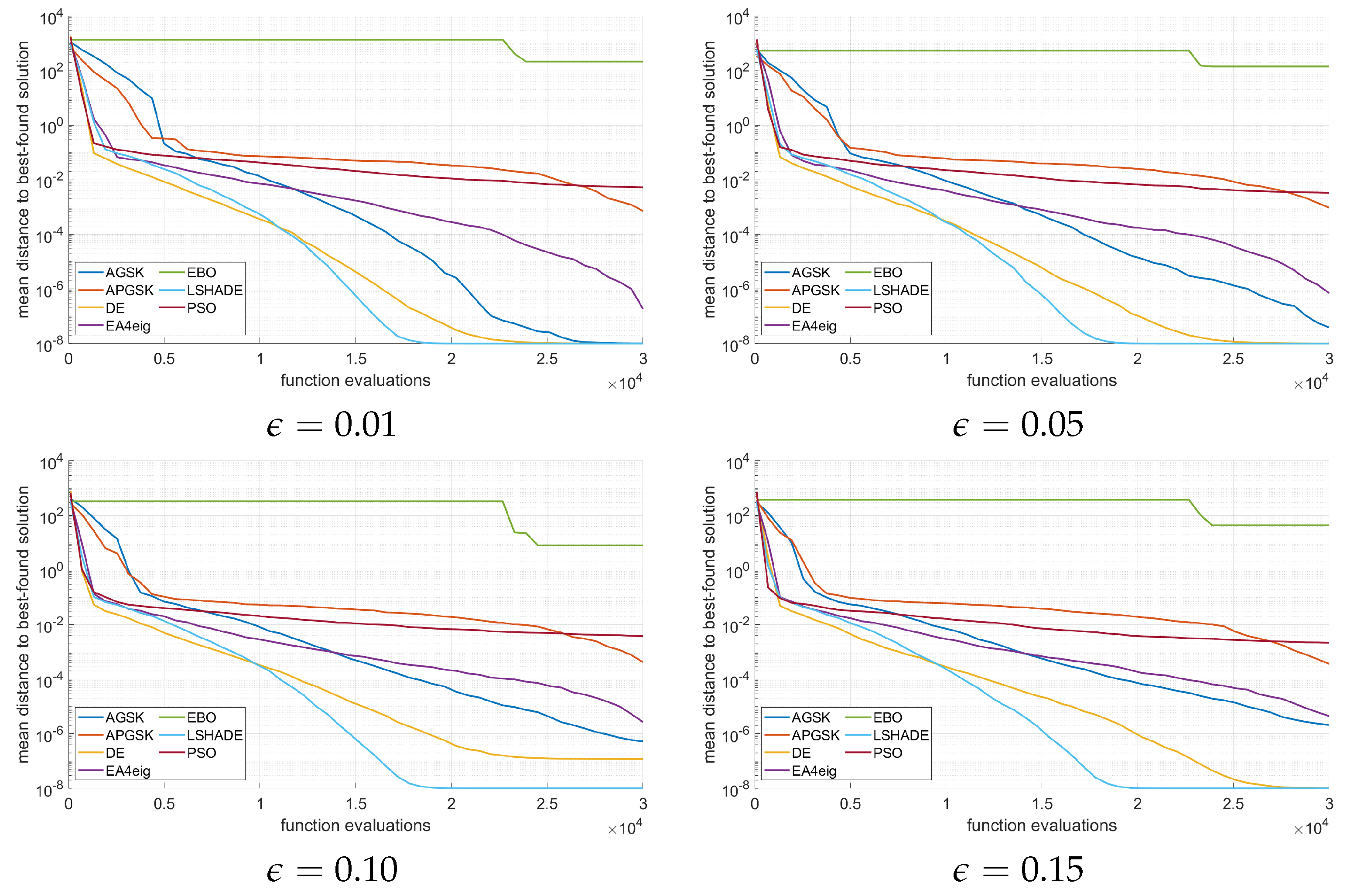
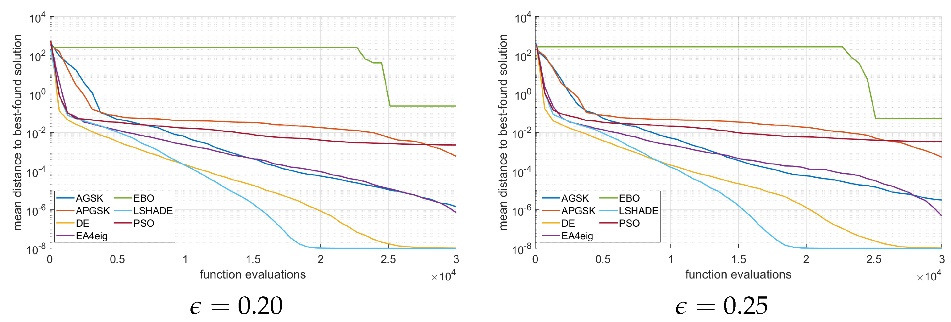
5.1. Performance Comparison of the Selected Methods

We first evaluated the performance of the selected methods on the deterministic case. In the analysis of the results, we decided to truncate the obtained best-found objective values to the seventh decimal place. The results of the computations (the statistics of the 20 independent runs) are summarized in

Table 3. Statistics of the 20 runs of the selected methods on the deterministic case.

	AGSK	APGSKI	DE	EA4eig	EBO	LSHADE	PSO
min	−1.2593538	−1.2593538	−1.2593538	−1.2593538	−1.2593538	−1.2593538	−1.2546087
mean	−1.2593538	−1.2593538	−1.2593538	−1.2593538	−1.2593538	−1.2593538	−1.2513056
max	−1.2593538	−1.2593538	−1.2593538	−1.2593538	−1.2593536	−1.2593538	−1.2485806
std	0.000	0.000	0.000	0.000	4.472 × 10${}^{-8}$	0.000	1.594 × 10${}^{-3}$

. Here, we find that almost all of the selected methods, with the exception of the PSO, were able to find the same solution and, except for the EBO, all of the methods found this solution consistently. The unit transportation cost of this solution was $UTC=13.6$.

Next, we investigated the results of the computations on the CCO model, which are reported in

Table 4. Statistics of the 20 runs of the selected methods on the CCO model.

$\mathit{ϵ}$		AGSK	APGSKI	DE	EA4eig	EBO	LSHADE	PSO
0.01	min	−0.9473943	−0.9473939	−0.9473943	−0.9473943	−0.8491422	−0.9473943	−0.9446069
	mean	−0.9473943	−0.9466775	−0.9473943	−0.9473941	212.9033097	−0.9473943	−0.9420872
	max	−0.9473943	−0.9403836	−0.9473943	−0.9473932	1043.7700147	−0.9473943	−0.9367206
	std	0.000	1.548 × 10${}^{-3}$	0.000	3.278 × 10${}^{-7}$	3.248 × 10${}^2$	0.000	2.166 × 10${}^{-3}$
0.05	min	−0.9991552	−0.9991529	−0.9991552	−0.9991552	−0.9691110	−0.9991552	−0.9982688
	mean	−0.9991552	−0.9982114	−0.9991552	−0.9991545	139.6795100	−0.9991552	−0.9958583
	max	−0.9991550	−0.9962695	−0.9991552	−0.9991514	607.0723893	−0.9991552	−0.9910965
	std	6.156 × 10${}^{-8}$	8.508 × 10${}^{-4}$	0.000	1.106 × 10${}^{-6}$	2.198 × 10${}^2$	0.000	1.668 × 10${}^{-3}$
0.10	min	−1.0291039	−1.0290552	−1.0291039	−1.0291039	−0.9795876	−1.0291039	−1.0279124
	mean	−1.0291034	−1.0286804	−1.0291038	−1.0291013	7.1408294	−1.0291039	−1.0252982
	max	−1.0291014	−1.0276915	−1.0291017	−1.0290916	159.0656498	−1.0291039	−1.0194222
	std	9.305 × 10${}^{-7}$	3.949 × 10${}^{-4}$	4.919 × 10${}^{-7}$	3.574 × 10${}^{-6}$	35.76	0.000	2.111 × 10${}^{-3}$
0.15	min	−1.0496266	−1.0496254	−1.0496266	−1.0496266	−1.0363353	−1.0496266	−1.0492396
	mean	−1.0496245	−1.0492608	−1.0496266	−1.0496221	42.7607508	−1.0496266	−1.0474384
	max	−1.0496125	−1.0479015	−1.0496266	−1.0496049	871.4141031	−1.0496266	−1.0431568
	std	3.512 × 10${}^{-6}$	4.669 × 10${}^{-4}$	0.000	6.710 × 10${}^{-6}$	1.950 × 10${}^2$	0.000	1.631 × 10${}^{-3}$
0.20	min	−1.0679705	−1.0679607	−1.0679705	−1.0679705	−1.0284986	−1.0679705	−1.0675095
	mean	−1.0679691	−1.0673805	−1.0679705	−1.0679699	−0.8312606	−1.0679705	−1.0657167
	max	−1.0679652	−1.0660410	−1.0679705	−1.0679684	1.5861289	−1.0679705	−1.0628487
	std	1.900 × 10${}^{-6}$	6.352 × 10${}^{-4}$	0.000	7.343 × 10${}^{-7}$	5.802 × 10${}^{-1}$	0.000	1.160 × 10${}^{-3}$
0.25	min	−1.0843175	−1.0843083	−1.0843175	−1.0843175	−1.0461846	−1.0843175	−1.0833582
	mean	−1.0843142	−1.0837891	−1.0843175	−1.0843170	−1.0317051	−1.0843175	−1.0809449
	max	−1.0843052	−1.0817133	−1.0843175	−1.0843145	−0.9836282	−1.0843175	−1.0772805
	std	4.584 × 10${}^{-6}$	6.152 × 10${}^{-4}$	0.000	7.545 × 10${}^{-7}$	1.475 × 10${}^{-2}$	0.000	1.761 × 10${}^{-3}$

. Here, the situation changed substantially to the deterministic case. The only method that could consistently find the best solution with the available computational budget was the LSHADE algorithm. The second method that was also very consistent in finding the best solution was DE—the only instances where it was not successful were for $ϵ=0.10$. One thing to notice is the quite bad performance of the EBO, which in many cases failed to find a feasible solution, which resulted in large values of the objective function (the details on the used penalization method can be found in [45]).

The convergence plots of the average function values of the selected methods to the best-found solution on the CCO models are depicted in Figure 1, where the differences smaller than 1 × 10⁻⁸ were neglected. Here, we can find some interesting insights into the suitability of the different methods for solving the CCO model. Although the DE algorithm has the best convergence in the first 10,000 iterations, it is eventually overtaken by the LSHADE, which dominates the rest of the computational budget. The third and fourth best methods were the AGSK and the EA4eig. We can find that the problems with larger values of $ϵ$ become more difficult, which is especially noticeable in the convergence of the AGSK (but also the other methods have their convergence negatively affected by larger values of $ϵ$). Also interesting is the fact that the “improved” version of the AGSK, the APGSKI method performed significantly worse than its predecessor and was only barely better than the PSO.

To perform a solid statistical comparison of the selected algorithms on the CCO model, we followed the guidelines published in [60]. First, we used the Kruskall–Wallis test to find if significant differences are present among all the algorithms for the different values of $ϵ$. The p-values for this test were [1.22 × 10${}^{-23}$, 2.58 × 10${}^{-23}$, 6.50 × 10${}^{-22}$, 8.81 × 10${}^{-22}$, 6.02 × 10${}^{-22}$, and 7.12 × 10${}^{-23}$] for the six studied values of $ϵ=[0.01,0.05,0.10,0.20]$, respectively. As all these p-values were much lower than the recommended confidence level $\alpha =0.05$, we can state that there are statistically significant differences between the selected methods. Furthermore, we utilized the Wilcoxon signed-rank test to find out whether statistically significant differences exist between the best algorithm (the LSHADE algorithm) and the other selected methods. Once the pairwise p-values were obtained, we applied the Holm–Bonferroni [79] correction method which counteracts the effect of multiple comparisons by controlling the family-wise error rate [80]. The results of the analysis are presented in

Table 5. Statistical analysis of the comparison of the selected methods.

		$ϵ=0.01$		$ϵ=0.05$		$ϵ=0.10$
		p	$p^{*}$	p	$p^{*}$	p	$p^{*}$
LSHADE vs other methods	DE	1.00	1.00 ✗	1.00	1.00 ✗	1.00	1.00 ✗
	AGSK	1.00	1.00 ✗	5.00 × 10${}^{-1}$	1.00 ✗	3.91 × 10${}^{-3}$	7.81 × 10${}^{-3}$
	EA4eig	3.13 × 10${}^{-2}$	9.38 × 10${}^{-2}$ ✗	9.77 × 10${}^{-4}$	2.93 × 10${}^{-3}$	1.22 × 10${}^{-4}$	3.66 × 10${}^{-4}$
	APGSKI	8.86 × 10${}^{-5}$	5.31 × 10${}^{-4}$	8.86 × 10${}^{-5}$	5.31 × 10${}^{-4}$	8.86 × 10${}^{-5}$	5.31 × 10${}^{-4}$
	PSO	8.86 × 10${}^{-5}$	5.31 × 10${}^{-4}$	8.86 × 10${}^{-5}$	5.31 × 10${}^{-4}$	8.86 × 10${}^{-5}$	5.31 × 10${}^{-4}$
	EBO	8.86 × 10${}^{-5}$	4.43 × 10${}^{-4}$	8.86 × 10${}^{-5}$	4.43 × 10${}^{-4}$	8.86 × 10${}^{-5}$	4.43 × 10${}^{-4}$
		$ϵ=0.15$		$ϵ=0.20$		$ϵ=0.25$
		p	$p^{*}$	p	$p^{*}$	p	$p^{*}$
LSHADE vs other methods	DE	1.00	1.00 ✗	1.00	1.00 ✗	1.00	1.00 ✗
	AGSK	6.10 × 10${}^{-5}$	3.66 × 10${}^{-4}$	1.22 × 10${}^{-4}$	3.66 × 10${}^{-4}$	1.24 × 10${}^{-4}$	3.73 × 10${}^{-4}$
	EA4eig	2.90 × 10${}^{-4}$	5.80 × 10${}^{-4}$	2.44 × 10${}^{-4}$	4.88 × 10${}^{-4}$	1.68 × 10${}^{-4}$	3.73 × 10${}^{-4}$
	APGSKI	8.86 × 10${}^{-5}$	4.43 × 10${}^{-4}$	8.86 × 10${}^{-5}$	5.31 × 10${}^{-4}$	8.86 × 10${}^{-5}$	5.31 × 10${}^{-4}$
	PSO	8.86 × 10${}^{-5}$	4.43 × 10${}^{-4}$	8.86 × 10${}^{-5}$	5.31 × 10${}^{-4}$	8.86 × 10${}^{-5}$	5.31 × 10${}^{-4}$
	EBO	8.86 × 10${}^{-5}$	3.54 × 10${}^{-4}$	8.86 × 10${}^{-5}$	4.43 × 10${}^{-4}$	8.86 × 10${}^{-5}$	4.43 × 10${}^{-4}$

p: p-value computed by the Wilcoxon text $p^{*}$: p-value corrected with the Holm–Bonferroni procedure ✗: statistical differences do not exist with significance level $\alpha =0.05$.

. We can see that, in all cases, the LSHADE and the DE algorithms were equivalent. The AGSK algorithm was also found to be as good as the LSHADE on the $ϵ=0.01$ and $ϵ=0.05$ instances. The last algorithm that was as good as the LSHADE on one instance was the EA4eig on $ϵ=0.01$.

When looking at the results, we can find interesting parallels between our findings and the results of other studies. The observation that PSO does relatively well at the very beginning of the search and the DE-type methods excel for larger computational budgets was also identified in [81]. The relatively poorer performance of some of the methods that were among the best-performing ones in the CEC Competitions (EA4Eig, AGSK, AGSKI, and, most notably, EBO) probably comes down to these methods being fine-tuned for the particular competition [82,83]. On the other hand, the excellent performance of LSHADE should not be as unexpected, as this method (and similar DE hybrids) was found to be among the best-performing ones on a variety of different problems [9,63,84,85,86]. The surprising competence of the “old” DE method for various engineering problems was also found in [9,68,85] and should be a point of further investigation.

One of the natural limitations of the presented study is that the performance comparison is valid only for the studied problem setting. Finding the reasons why certain methods outperform others on different problems is an extremely important question that is closely tied to one of the most debated topics in evolutionary computation (and also deterministic optimization) communities—efficient algorithmic selection [87], i.e., how to decide (based on some problem characteristics) what kind of algorithm will perform well. Although one can find efficient methods, for instance, for some convex optimization problems, for the general nonconvex (and black-box) ones (such as the one discussed in this paper), no such analysis is yet to be found. One could invoke a parallel to the no-free-lunch theorem, but that was found not to be exactly the case for continuous problems [88]. In this context, it is almost impossible to say why certain methods did not perform very well (or outperformed others) on a given problem.

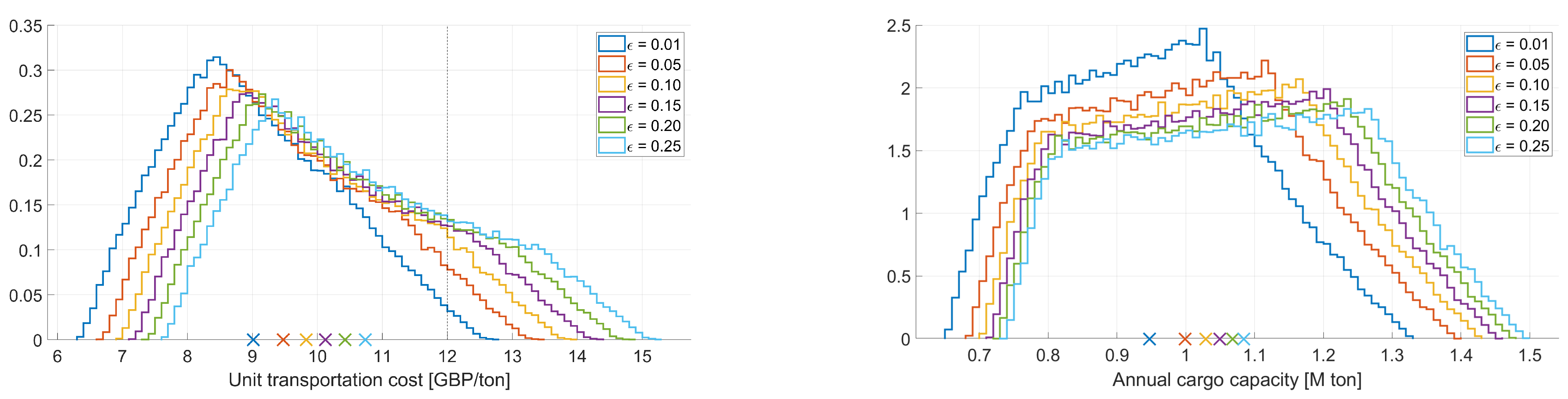
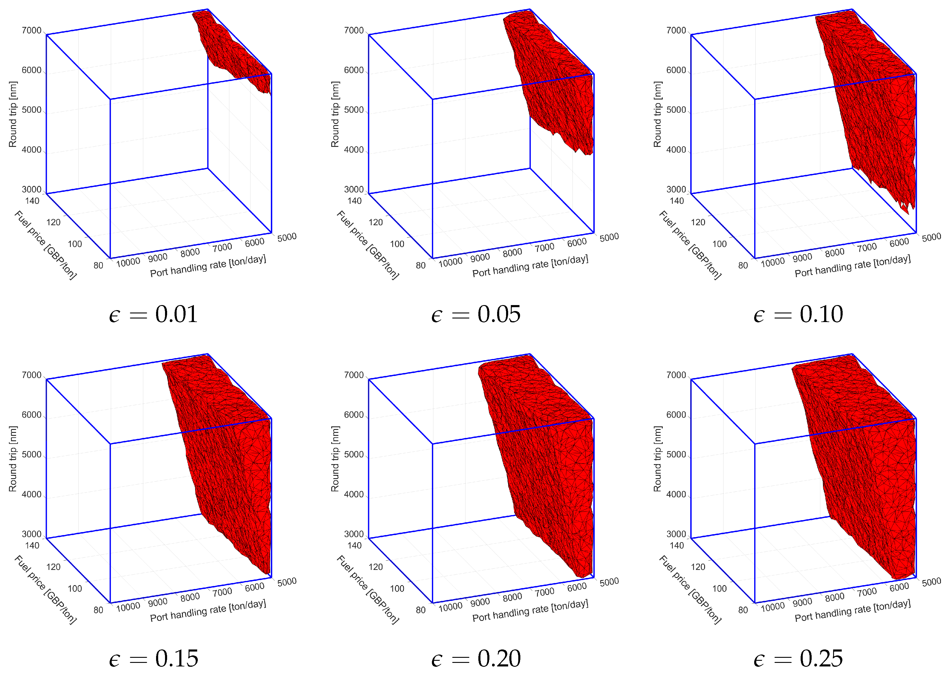
5.2. Evaluation of the Best-Found Solutions

In the next step, we investigated the best-found solutions for the different instances. The values of the optimization variables for these solutions are reported in

Table 6. Values of the optimization variables for the best-found solutions for the different instances.

	$\mathit{ϵ}$
Variable	Symbol	0.01	0.05	0.1	0.15	0.2	0.25	Deterministic
Length	L	275.5554	295.3920	308.5694	318.4319	327.2925	334.3526	412.3332
Beam	B	45.9271	49.2330	51.4290	53.0728	54.5495	55.7262	68.7358
Depth	D	24.9640	26.6760	27.8068	28.6498	29.4037	30.0000	30.0000
Draft	T	18.1749	19.3732	20.1648	20.7549	21.2826	21.7000	21.7010
Block coefficient	$C_B$	0.7500	0.7500	0.7500	0.7500	0.7500	0.7500	0.7500
Cruise speed	$V_k$	14.0000	14.0000	14.0051	14.0236	14.1336	14.4225	18.0000

. We can see that, as the value of $ϵ$ increases, the size of the conceptual bulk carrier ship (defined by the variables $L,B,D,$ and T) also increases. The depth variable D even gets to its upper bound for $ϵ=0.25$. The cruise speed variable $V_k$ remains close to its lower bound, as it has a high impact on the unit transportation costs. The only variable that has the same value for all instances is the block coefficient $C_B$ with the value of its upper bound. We can compare these solutions to the deterministic one, which does not take into account the unit transportation costs. Here, the resulting size of the ship is even larger, and it is expected to move at the maximum allowable cruise speed (this should be expected, as this setup is only designed to maximize the annual cargo capacity).

The effect of the chosen values of $ϵ$ on the distributions of the unit transportation cost $UTC$ and annual cargo capacity $ACC$ are shown in Figure 2. Unsurprisingly, as the value of $ϵ$ increases, we see a shift of the distribution of the unit transportation costs to higher values, which can also be seen in the shift of the expected values to the right. Note that the area under the probability distribution functions for values larger than the chosen threshold $THR=12$ must be $\le ϵ$ (which is the effect of the chance constraint). A similar shift can be seen in the distribution of the annual cargo capacity (which was the objective we wanted to maximize).

The last bit of analysis we will discuss is the structure of the scenarios, for which the chance-constraint (48) was violated for different values of $ϵ$. The visualization of these scenarios was performed by using the alpha shapes [89], and is shown in Figure 3. From these visualizations, we can infer that the uncertain parameter that has the largest negative effect on the unit transportation cost $UTC$ was the port handling rate $PHR$, as the violated scenarios for all values of $ϵ$ had values on the lower bound of $PHR$. The second uncertain parameter that had a slightly lower impact was round trip miles $RTM$. The impact of the fuel price $FP$ was the lowest of the three (it might not be clearly visible from Figure 3, but it was measurable).

Naturally, the provided analysis is only valid for the choices of distributions of the uncertain parameters and variable ranges in Table 1 and Table 2. However, the general framework of the optimization model (7)–(48), with the CCO approach and the analysis of the performance of the different methods, should be readily transferable into modified settings (choosing other distributions, having dependence in the distributions, considering different variable ranges, etc.).

6. Conclusions

In this paper, we introduced the extension of the conceptual bulk carrier design model with the scenario-based chance-constrained approach that takes into account different sources of uncertainty that can influence the design. We performed an extensive numerical comparison of selected (canonical and state-of-the-art) metaheuristic algorithms on the proposed model and found that the chance-constrained extension made the resulting problem significantly more challenging, even for the state-of-the-art evolutionary computation techniques. We also investigated the effect of the chance-constraint parameter $ϵ$ (i.e., the probability of the violation of the chance constraint). Interestingly, the two best-performing methods (the LSHADE and the DE algorithm) were not among the most recent ones (and the DE is almost three decades old). For the overall best-found solution, we conducted a computational analysis of the effect of $ϵ$ on the distributions of unit transportation costs and annual cargo capacity, the relationship between the two, and the relationship between the three uncertain parameters in the violated scenarios.

There are several interesting possibilities for additional extensions and future work. The CCO problem could be posed as a multi-objective optimization problem instead, and the quality of the Pareto front (maximizing the annual cargo capacity and minimizing the probability of violating the chance constraint) of different algorithms could be investigated. It would also be interesting to study the differences in solutions obtained by the CCO and the robust/reliability-based approaches for different kinds of probability distributions of the uncertain parameters. Another direction might lie in the utilization and comparison of DIRECT-type methods and various surrogate-assisted techniques. Lastly, it would be interesting to investigate possible extensions of other engineering problems that are currently used for benchmarking metaheuristics into the chance-constrained (or other stochastic) formulations utilized in this paper.

References

1. Diez, M.; Peri, D. Robust optimization for ship conceptual design. Ocean. Eng. 2010, 37, 966–977. [Google Scholar] [CrossRef]
2. Kochenderfer, M.J.; Wheeler, T.A. Algorithms for Optimization; Mit Press: Cambridge, MA, USA, 2019. [Google Scholar]
3. Ben-Tal, A.; El Ghaoui, L.; Nemirovski, A. Robust Optimization; Princeton University Press: Princeton, NJ, USA, 2009; Volume 28. [Google Scholar]
4. Prékopa, A. Stochastic Programming; Springer Science & Business Media: Berlin/Heidelberg, Germany, 2013; Volume 324. [Google Scholar]
5. Shafer, G. Dempster-shafer theory. Encycl. Artif. Intell. 1992, 1, 330–331. [Google Scholar]
6. Zimmermann, H.J. Fuzzy set theory. Wiley Interdiscip. Rev. Comput. Stat. 2010, 2, 317–332. [Google Scholar] [CrossRef]
7. Dubois, D.; Prade, H. Possibility theory and its applications: Where do we stand? In Springer Handbook of Computational Intelligence; Springer: Berlin/Heidelberg, Germany, 2015; pp. 31–60. [Google Scholar]
8. Ben-Haim, Y. Info-Gap Decision Theory: Decisions under Severe Uncertainty; Elsevier: Amsterdam, The Netherlands, 2006. [Google Scholar]
9. Kudela, J. A critical problem in benchmarking and analysis of evolutionary computation methods. Nat. Mach. Intell. 2022, 4, 1238–1245. [Google Scholar] [CrossRef]
10. Tzanetos, A.; Blondin, M. A qualitative systematic review of metaheuristics applied to tension/compression spring design problem: Current situation, recommendations, and research direction. Eng. Appl. Artif. Intell. 2023, 118, 105521. [Google Scholar] [CrossRef]
11. Žufan, P.; Bidlo, M. Advances in evolutionary optimization of quantum operators. Mendel 2021, 27, 12–22. [Google Scholar] [CrossRef]
12. Abu Khurma, R.; Aljarah, I.; Sharieh, A.; Abd Elaziz, M.; Damaševičius, R.; Krilavičius, T. A review of the modification strategies of the nature inspired algorithms for feature selection problem. Mathematics 2022, 10, 464. [Google Scholar] [CrossRef]
13. Akinola, O.O.; Ezugwu, A.E.; Agushaka, J.O.; Zitar, R.A.; Abualigah, L. Multiclass feature selection with metaheuristic optimization algorithms: A review. Neural Comput. Appl. 2022, 34, 19751–19790. [Google Scholar] [CrossRef]
14. Ma, J.; Xia, D.; Wang, Y.; Niu, X.; Jiang, S.; Liu, Z.; Guo, H. A comprehensive comparison among metaheuristics (MHs) for geohazard modeling using machine learning: Insights from a case study of landslide displacement prediction. Eng. Appl. Artif. Intell. 2022, 114, 105150. [Google Scholar] [CrossRef]
15. Muller, J. Improving initial aerofoil geometry using aerofoil particle swarm optimisation. Mendel 2022, 28, 63–67. [Google Scholar] [CrossRef]
16. Febrianti, W.; Sidarto, K.A.; Sumarti, N. Approximate Solution for Barrier Option Pricing Using Adaptive Differential Evolution With Learning Parameter. Mendel 2022, 28, 76–82. [Google Scholar] [CrossRef]
17. Jones, D.R.; Martins, J.R. The DIRECT algorithm: 25 years Later. J. Glob. Optim. 2021, 79, 521–566. [Google Scholar] [CrossRef]
18. Kudela, J.; Matousek, R. Recent advances and applications of surrogate models for finite element method computations: A review. Soft Comput. 2022, 26, 13709–13733. [Google Scholar] [CrossRef]
19. Greiner, H. Robust optical coating design with evolutionary strategies. Appl. Opt. 1996, 35, 5477–5483. [Google Scholar] [CrossRef] [PubMed]
20. Wiesmann, D.; Hammel, U.; Back, T. Robust design of multilayer optical coatings by means of evolutionary algorithms. IEEE Trans. Evol. Comput. 1998, 2, 162–167. [Google Scholar] [CrossRef]
21. Branke, J. Creating robust solutions by means of evolutionary algorithms. In Proceedings of the Parallel Problem Solving from Nature—PPSN V: 5th International Conference, Amsterdam, The Netherlands, 27–30 September 1998; Proceedings 5; Springer: Berlin/Heidelberg, Germany, 1998; pp. 119–128. [Google Scholar]
22. Tsutsui, S.; Ghosh, A. Genetic algorithms with a robust solution searching scheme. IEEE Trans. Evol. Comput. 1997, 1, 201–208. [Google Scholar] [CrossRef]
23. Forouraghi, B. A genetic algorithm for multiobjective robust design. Appl. Intell. 2000, 12, 151–161. [Google Scholar] [CrossRef]
24. Loughlin, D.H.; Ranjithan, S.R. Chance-constrained optimization using genetic algorithms: An application in air quality management. In Proceedings of the Bridging the Gap: Meeting the World’s Water and Environmental Resources Challenges, Orlando, FL, USA, 20–24 May 2001; pp. 1–9. [Google Scholar]
25. Asafuddoula, M.; Singh, H.K.; Ray, T. Six-sigma robust design optimization using a many-objective decomposition-based evolutionary algorithm. IEEE Trans. Evol. Comput. 2014, 19, 490–507. [Google Scholar] [CrossRef]
26. Paenke, I.; Branke, J.; Jin, Y. Efficient search for robust solutions by means of evolutionary algorithms and fitness approximation. IEEE Trans. Evol. Comput. 2006, 10, 405–420. [Google Scholar] [CrossRef]
27. Kim, C.; Choi, K.K. Reliability-based design optimization using response surface method with prediction interval estimation. ASME J. Mech. Des. 2008, 130, 121401. [Google Scholar] [CrossRef]
28. Ma, W.; Ma, D.; Ma, Y.; Zhang, J.; Wang, D. Green maritime: A routing and speed multi-objective optimization strategy. J. Clean. Prod. 2021, 305, 127179. [Google Scholar] [CrossRef]
29. Fagerholt, K.; Gausel, N.T.; Rakke, J.G.; Psaraftis, H.N. Maritime routing and speed optimization with emission control areas. Transp. Res. Part C Emerg. Technol. 2015, 52, 57–73. [Google Scholar] [CrossRef]
30. Andersson, H.; Fagerholt, K.; Hobbesland, K. Integrated maritime fleet deployment and speed optimization: Case study from RoRo shipping. Comput. Oper. Res. 2015, 55, 233–240. [Google Scholar] [CrossRef]
31. Cheaitou, A.; Cariou, P. Greening of maritime transportation: A multi-objective optimization approach. Ann. Oper. Res. 2019, 273, 501–525. [Google Scholar] [CrossRef]
32. Zhou, C.; Ma, N.; Cao, X.; Lee, L.H.; Chew, E.P. Classification and literature review on the integration of simulation and optimization in maritime logistics studies. IISE Trans. 2021, 53, 1157–1176. [Google Scholar] [CrossRef]
33. Jin, X.; Duan, Z.; Song, W.; Li, Q. Container stacking optimization based on Deep Reinforcement Learning. Eng. Appl. Artif. Intell. 2023, 123, 106508. [Google Scholar] [CrossRef]
34. Zeng, C.; Wang, J.B.; Ding, C.; Zhang, H.; Lin, M.; Cheng, J. Joint optimization of trajectory and communication resource allocation for unmanned surface vehicle enabled maritime wireless networks. IEEE Trans. Commun. 2021, 69, 8100–8115. [Google Scholar] [CrossRef]
35. Sen, P.; Yang, J.B. Multiple Criteria Decision Support in Engineering Design; Springer Science & Business Media: Berlin/Heidelberg, Germany, 1998. [Google Scholar]
36. Parsons, M.G.; Scott, R.L. Formulation of multicriterion design optimization problems for solution with scalar numerical optimization methods. J. Ship Res. 2004, 48, 61–76. [Google Scholar] [CrossRef]
37. Hart, C.G.; Vlahopoulos, N. An integrated multidisciplinary particle swarm optimization approach to conceptual ship design. Struct. Multidiscip. Optim. 2010, 41, 481–494. [Google Scholar] [CrossRef]
38. Serani, A.; Leotardi, C.; Iemma, U.; Campana, E.F.; Fasano, G.; Diez, M. Parameter selection in synchronous and asynchronous deterministic particle swarm optimization for ship hydrodynamics problems. Appl. Soft Comput. 2016, 49, 313–334. [Google Scholar] [CrossRef]
39. Chen, X.; Diez, M.; Kandasamy, M.; Zhang, Z.; Campana, E.F.; Stern, F. High-fidelity global optimization of shape design by dimensionality reduction, metamodels and deterministic particle swarm. Eng. Optim. 2015, 47, 473–494. [Google Scholar] [CrossRef]
40. Serani, A.; Fasano, G.; Liuzzi, G.; Lucidi, S.; Iemma, U.; Campana, E.F.; Stern, F.; Diez, M. Ship hydrodynamic optimization by local hybridization of deterministic derivative-free global algorithms. Appl. Ocean. Res. 2016, 59, 115–128. [Google Scholar] [CrossRef]
41. Campana, E.F.; Diez, M.; Liuzzi, G.; Lucidi, S.; Pellegrini, R.; Piccialli, V.; Rinaldi, F.; Serani, A. A multi-objective DIRECT algorithm for ship hull optimization. Comput. Optim. Appl. 2018, 71, 53–72. [Google Scholar] [CrossRef]
42. Diez, M.; Campana, E.F.; Stern, F. Stochastic optimization methods for ship resistance and operational efficiency via CFD. Struct. Multidiscip. Optim. 2018, 57, 735–758. [Google Scholar] [CrossRef]
43. Serani, A.; Stern, F.; Campana, E.F.; Diez, M. Hull-form stochastic optimization via computational-cost reduction methods. Eng. Comput. 2022, 38, 2245–2269. [Google Scholar] [CrossRef]
44. Calafiore, G.; Campi, M.C. Uncertain convex programs: Randomized solutions and confidence levels. Math. Program. 2005, 102, 25–46. [Google Scholar] [CrossRef]
45. Kudela, J. Zenodo Repository: Chance-Constrained Optimization Formulation for Conceptual Ship Design: A Comparison of Metaheuristic Algorithms. 2023. Available online: https://zenodo.org/records/8178768 (accessed on 9 October 2023).
46. Rockafellar, R.T.; Uryasev, S. Optimization of conditional value-at-risk. J. Risk 2000, 2, 21–42. [Google Scholar] [CrossRef]
47. Rockafellar, R.T.; Royset, J.O. On buffered failure probability in design and optimization of structures. Reliab. Eng. Syst. Saf. 2010, 95, 499–510. [Google Scholar] [CrossRef]
48. Charnes, A.; Cooper, W.W.; Symonds, G.H. Cost horizons and certainty equivalents: An approach to stochastic programming of heating oil. Manag. Sci. 1958, 4, 235–263. [Google Scholar] [CrossRef]
49. Nemirovski, A. On safe tractable approximations of chance constraints. Eur. J. Oper. Res. 2012, 219, 707–718. [Google Scholar] [CrossRef]
50. Kudela, J.; Popela, P. Pool & discard algorithm for chance constrained optimization problems. IEEE Access 2020, 8, 79397–79407. [Google Scholar]
51. Neumann, A.; Neumann, F. Optimising monotone chance-constrained submodular functions using evolutionary multi-objective algorithms. In Proceedings of the International Conference on Parallel Problem Solving from Nature; Springer: Berlin/Heidelberg, Germany, 2020; pp. 404–417. [Google Scholar]
52. Doerr, B.; Doerr, C.; Neumann, A.; Neumann, F.; Sutton, A. Optimization of chance-constrained submodular functions. In Proceedings of the AAAI Conference on Artificial Intelligence, New York, NY, USA, 7–12 February 2020; Volume 34, pp. 1460–1467. [Google Scholar]
53. Xie, Y.; Neumann, A.; Neumann, F. Specific single-and multi-objective evolutionary algorithms for the chance-constrained knapsack problem. In Proceedings of the 2020 Genetic and Evolutionary Computation Conference, Cancun, Mexico, 8–12 July 2020; pp. 271–279. [Google Scholar]
54. Campi, M.C.; Garatti, S. The exact feasibility of randomized solutions of uncertain convex programs. SIAM J. Optim. 2008, 19, 1211–1230. [Google Scholar] [CrossRef]
55. Camacho-Villalón, C.L.; Dorigo, M.; Stützle, T. The intelligent water drops algorithm: Why it cannot be considered a novel algorithm. Swarm Intell. 2019, 13, 173–192. [Google Scholar] [CrossRef]
56. Camacho Villalón, C.L.; Stützle, T.; Dorigo, M. Grey wolf, firefly and bat algorithms: Three widespread algorithms that do not contain any novelty. In Proceedings of the International Conference on Swarm Intelligence; Springer: Berlin/Heidelberg, Germany, 2020; pp. 121–133. [Google Scholar]
57. Weyland, D. A rigorous analysis of the harmony search algorithm: How the research community can be misled by a “novel” methodology. Int. J. Appl. Metaheuristic Comput. (IJAMC) 2010, 1, 50–60. [Google Scholar] [CrossRef]
58. Aranha, C.; Camacho Villalón, C.L.; Campelo, F.; Dorigo, M.; Ruiz, R.; Sevaux, M.; Sörensen, K.; Stützle, T. Metaphor-based metaheuristics, a call for action: The elephant in the room. Swarm Intell. 2022, 16, 1–6. [Google Scholar] [CrossRef]
59. Kudela, J. Commentary on:“STOA: A bio-inspired based optimization algorithm for industrial engineering problems”[EAAI, 82 (2019), 148–174] and “Tunicate Swarm Algorithm: A new bio-inspired based metaheuristic paradigm for global optimization”[EAAI, 90 (2020), no. 103541]. Eng. Appl. Artif. Intell. 2022, 113, 104930. [Google Scholar]
60. LaTorre, A.; Molina, D.; Osaba, E.; Poyatos, J.; Del Ser, J.; Herrera, F. A prescription of methodological guidelines for comparing bio-inspired optimization algorithms. Swarm Evol. Comput. 2021, 67, 100973. [Google Scholar] [CrossRef]
61. Mohamed, A.W.; Hadi, A.A.; Mohamed, A.K. Gaining-sharing knowledge based algorithm for solving optimization problems: A novel nature-inspired algorithm. Int. J. Mach. Learn. Cybern. 2020, 11, 1501–1529. [Google Scholar] [CrossRef]
62. Mohamed, A.W.; Hadi, A.A.; Mohamed, A.K.; Awad, N.H. Evaluating the performance of adaptive gaining-sharing knowledge based algorithm on CEC 2020 benchmark problems. In Proceedings of the 2020 IEEE Congress on Evolutionary Computation (CEC), Glasgow, UK, 19–24 July 2020; pp. 1–8. [Google Scholar]
63. Kůdela, J.; Juříček, M.; Parák, R. A Collection of Robotics Problems for Benchmarking Evolutionary Computation Methods. In Proceedings of the International Conference on the Applications of Evolutionary Computation (Part of EvoStar); Springer: Berlin/Heidelberg, Germany, 2023; pp. 364–379. [Google Scholar]
64. Sallam, K.M.; Elsayed, S.M.; Chakrabortty, R.K.; Ryan, M.J. Improved multi-operator differential evolution algorithm for solving unconstrained problems. In Proceedings of the 2020 IEEE Congress on Evolutionary Computation (CEC), Glasgow, UK, 19–24 July 2020; pp. 1–8. [Google Scholar]
65. Storn, R.; Price, K. Differential evolution—A simple and efficient heuristic for global optimization over continuous spaces. J. Glob. Optim. 1997, 11, 341–359. [Google Scholar] [CrossRef]
66. Das, S.; Suganthan, P.N. Differential evolution: A survey of the state-of-the-art. IEEE Trans. Evol. Comput. 2010, 15, 4–31. [Google Scholar] [CrossRef]
67. Pant, M.; Zaheer, H.; Garcia-Hernandez, L.; Abraham, A. Differential Evolution: A review of more than two decades of research. Eng. Appl. Artif. Intell. 2020, 90, 103479. [Google Scholar]
68. Bujok, P.; Lacko, M.; Kolenovský, P. Differential Evolution and Engineering Problems. Mendel 2023, 29, 45–54. [Google Scholar] [CrossRef]
69. Kůdela, J.; Matoušek, R. Combining Lipschitz and RBF surrogate models for high-dimensional computationally expensive problems. Inf. Sci. 2023, 619, 457–477. [Google Scholar] [CrossRef]
70. Hansen, N.; Müller, S.D.; Koumoutsakos, P. Reducing the time complexity of the derandomized evolution strategy with covariance matrix adaptation (CMA-ES). Evol. Comput. 2003, 11, 1–18. [Google Scholar] [CrossRef]
71. Tanabe, R.; Fukunaga, A.S. Improving the search performance of SHADE using linear population size reduction. In Proceedings of the 2014 IEEE Congress on Evolutionary Computation (CEC), Beijing, China, 6–1 July 2014; pp. 1658–1665. [Google Scholar]
72. Piotrowski, A.P.; Napiorkowski, J.J. Step-by-step improvement of JADE and SHADE-based algorithms: Success or failure? Swarm Evol. Comput. 2018, 43, 88–108. [Google Scholar] [CrossRef]
73. Kennedy, J.; Eberhart, R. Particle swarm optimization. In Proceedings of the ICNN’95—International Conference on Neural Networks, Perth, WA, Australia, 27 December–1 November 1995; Volume 4, pp. 1942–1948. [Google Scholar]
74. Piotrowski, A.P.; Napiorkowski, J.J.; Piotrowska, A.E. Particle swarm optimization or differential evolution—A comparison. Eng. Appl. Artif. Intell. 2023, 121, 106008. [Google Scholar] [CrossRef]
75. Poli, R.; Kennedy, J.; Blackwell, T. Particle swarm optimization: An overview. Swarm Intell. 2007, 1, 33–57. [Google Scholar] [CrossRef]
76. Wang, D.; Tan, D.; Liu, L. Particle swarm optimization algorithm: An overview. Soft Comput. 2018, 22, 387–408. [Google Scholar] [CrossRef]
77. Piotrowski, A.P.; Napiorkowski, J.J.; Piotrowska, A.E. Population size in particle swarm optimization. Swarm Evol. Comput. 2020, 58, 100718. [Google Scholar] [CrossRef]
78. Kazikova, A.; Pluhacek, M.; Senkerik, R. Why tuning the control parameters of metaheuristic algorithms is so important for fair comparison? Mendel 2020, 26, 9–16. [Google Scholar] [CrossRef]
79. Holm, S. A simple sequentially rejective multiple test procedure. Scand. J. Stat. 1979, 65–70. [Google Scholar]
80. Aickin, M.; Gensler, H. Adjusting for multiple testing when reporting research results: The Bonferroni vs Holm methods. Am. J. Public Health 1996, 86, 726–728. [Google Scholar] [CrossRef]
81. Piotrowski, A.P.; Napiorkowski, M.J.; Napiorkowski, J.J.; Rowinski, P.M. Swarm intelligence and evolutionary algorithms: Performance versus speed. Inf. Sci. 2017, 384, 34–85. [Google Scholar] [CrossRef]
82. García-Martínez, C.; Gutiérrez, P.D.; Molina, D.; Lozano, M.; Herrera, F. Since CEC 2005 competition on real-parameter optimisation: A decade of research, progress and comparative analysis’s weakness. Soft Comput. 2017, 21, 5573–5583. [Google Scholar] [CrossRef]
83. Piotrowski, A.P.; Napiorkowski, J.J.; Piotrowska, A.E. How Much Do Swarm Intelligence and Evolutionary Algorithms Improve Over a Classical Heuristic From 1960? IEEE Access 2023, 11, 19775–19793. [Google Scholar] [CrossRef]
84. Bujok, P.; Tvrdík, J.; Poláková, R. Comparison of nature-inspired population-based algorithms on continuous optimisation problems. Swarm Evol. Comput. 2019, 50, 100490. [Google Scholar] [CrossRef]
85. Kudela, J.; Zalesak, M.; Charvat, P.; Klimes, L.; Mauder, T. Assessment of the performance of metaheuristic methods used for the inverse identification of effective heat capacity of phase change materials. Expert Syst. Appl. 2023, 122373. [Google Scholar] [CrossRef]
86. Kudela, J.; Matousek, R. New benchmark functions for single-objective optimization based on a zigzag pattern. IEEE Access 2022, 10, 8262–8278. [Google Scholar] [CrossRef]
87. Bäck, T.H.; Kononova, A.V.; van Stein, B.; Wang, H.; Antonov, K.A.; Kalkreuth, R.T.; de Nobel, J.; Vermetten, D.; de Winter, R.; Ye, F. Evolutionary Algorithms for Parameter Optimization—Thirty Years Later. Evol. Comput. 2023, 31, 81–122. [Google Scholar] [CrossRef]
88. Auger, A.; Teytaud, O. Continuous lunches are free plus the design of optimal optimization algorithms. Algorithmica 2010, 57, 121–146. [Google Scholar] [CrossRef]
89. Edelsbrunner, H.; Kirkpatrick, D.; Seidel, R. On the shape of a set of points in the plane. IEEE Trans. Inf. Theory 1983, 29, 551–559. [Google Scholar] [CrossRef]
Figure 1. Convergence plots of the average function values of the selected methods on the CCO models.
Computers 12 00225 g001aComputers 12 00225 g001b
Figure 2. Estimated probability distribution functions of the unit transportation cost (left) and annual cargo capacity (right) using the best-found solutions for the different instances. The expected values are shown as crosses.
Computers 12 00225 g002
Figure 3. Visualization of the violated scenarios (in red) for different values of ϵ . The blue lines delimit the ranges of the uncertain parameters.
Computers 12 00225 g003