
Mind Your Outcomes: The ΔQSD Paradigm for Quality-Centric Systems Development and Its Application to a Blockchain Case Study †

 , , , , and
Abstract
:1. Introduction
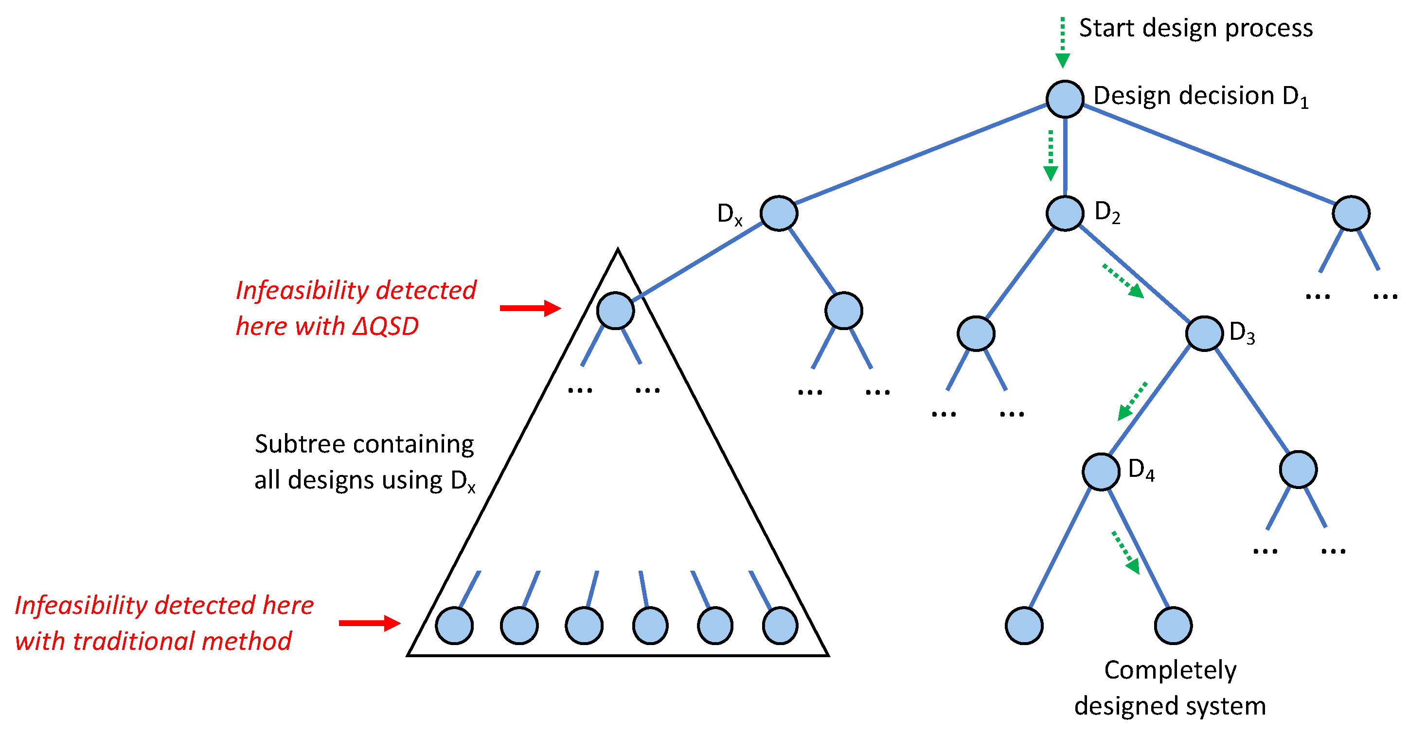
1.1. Motivation
- System requirements are often vague and/or contradictory, and they can change both during and after development;
- Complexity forces hierarchical decomposition of the problem, creating boundaries, including commercial boundaries with third-party suppliers, that may hinder optimal development and hide risks;
- Time pressure forces parallel development that may be at odds with that hierarchical decomposition, and it encourages leaving ‘tricky’ issues for later, when they tend to cause re-work and overruns and leave tail-risks;
- Cost and resource constraints force resources to be shared both within the system and with other systems (e.g., when network infrastructure or computing resources are shared); they may also require re-use of existing assets (own or third-party), introducing a degree of variability in the delivered performance;
- The performance of particular components or subsystems may be incompletely quantified;
- System performance and resource consumption may not scale linearly (which may not become apparent until moving from a lab/pilot phase to a wider deployment);
- At scale, exceptional events (transient communications and/or hardware issues) can no longer be treated as negligibly rare, and their effects and mitigation need to be considered along with the associated performance impacts.
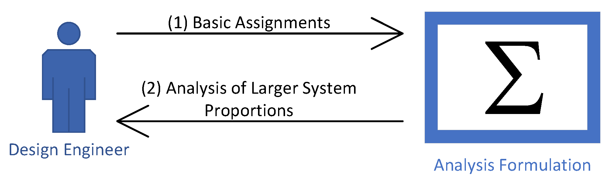
1.2. The SD Systems Development Paradigm
1.3. Main Contributions of this Paper
- Introduce SD, a formalism (Section 5) that focuses on rapidly exploring the performance consequences of design and implementation choices, where:
- (a)
- Performance is a first-class citizen, ensuring that we can focus on details relevant to performance behaviour;
- (b)
- The whole software development process is supported, from checking the feasibility of initial requirements to making decisions about subtle implementation choices and potential optimisations;
- (c)
- We can measure our choices against desired outcomes for individual users (customer experience);
- (d)
- Analysis of saturated systems is supported (where a “saturated system” is one with resources that have reached their limits, e.g., systems with high load or high congestion);
- (e)
- Analysis of failure is supported.
We use term-rewriting for formalising refinements (Definition 3 in Section 5) and denotational semantics for formalising timeliness analysis (Section 5.3) as well as load analysis (Section 5.4). - Describe key decisions made in the development process of a real system—i.e., the Cardano blockchain, which is presented as a running example—and show how SD is able to quickly rule out infeasible decisions, predict behaviour, and indicate design headroom (slack) to decision makers, architects, and developers (Section 4).
1.4. Structure of the Paper
- Section 2 introduces the running example that we will use throughout the paper: block diffusion in the Cardano blockchain.
- Section 3 defines the basic concepts that underlie the SD formalism: outcomes, outcome diagrams, and quality attenuation (). We also compare outcome diagrams with more traditional diagrams such as block diagrams.
- Section 4 gives a realistic example of the SD paradigm, showing a step-by-step design of block diffusion (introduced in Section 2) based on quality analysis. This example introduces the basic operations of SD in a tutorial fashion. The example uses realistic system parameters that allow us to compute predicted system behaviour.
- Section 5 gives the formal mathematical definition of SD and its main properties. With this formal definition, it is possible to validate the computations that are used by SD as well as to build tools based on SD.
- Section 6 gives a comprehensive discussion about related work from three different viewpoints: theoretical approaches for performance analysis (Section 6.1), performance design practices in distributed systems (Section 6.3), and programming languages and software engineering (Section 6.4).
- Section 7 summarises our conclusions, discusses some limitations of the paradigm, and describes our plans to further validate SD and to build a dedicated toolset for real-time distributed systems design that builds on the SD paradigm.
2. Running Example: Block Diffusion in the Cardano Blockchain
2.1. Key Design Decisions
- How frequently should blocks be produced? Proof-of-Work systems are limited in their throughput by the time taken to ‘crack’ the cryptographic puzzle; proof-of-stake systems do not have this limitation and so have the potential for much higher performance both in terms of the volume of transactions embedded into blocks and the time take for a transaction to be fully incorporated in the immutable part of the chain. Thus, the interval between blocks is a key parameter.
- How are nodes connected? It might seem that connecting every node to every other would minimise block diffusion time; however, the lack of any control over the number and capabilities of nodes makes this infeasible. Nodes can only be connected to a limited number of peer nodes; then, the number of connected peers and how they are chosen become important.
- How much data should be in a block? Increasing the amount of data in a block improves the overall throughput of the system but makes block diffusion slower.
- How should blocks be forwarded? Simply forwarding a new block to all connected nodes would seem to minimise delay, but this wastes resources, since a node may receive the same block from multiple peers. In the extreme case, this represents a potential denial-of-service attack. Splitting a block into a small header portion (sufficient for a node to decide whether it is new) and a larger body that a node can choose to download if it wishes mitigates this problem but adds an additional step into the forwarding process.
- How much time can be spent processing a block? Validating the contents of a block before forwarding it mitigates adversarial behaviour but can be computationally intensive, since the contents may be programs that need to be executed (called ‘smart contracts’); allowing more time for such processing permits more, and more complex, programs but makes block diffusion slower.
2.2. Formulating the Problem
3. Foundations
3.1. Outcomes
- Can be easily quantified without even a need for them to be named;
- Are beyond the design engineer’s control (and so may need to be quantified by external specification or measurement); or,
- Are ones for which the design engineer has intentionally left the details for later.
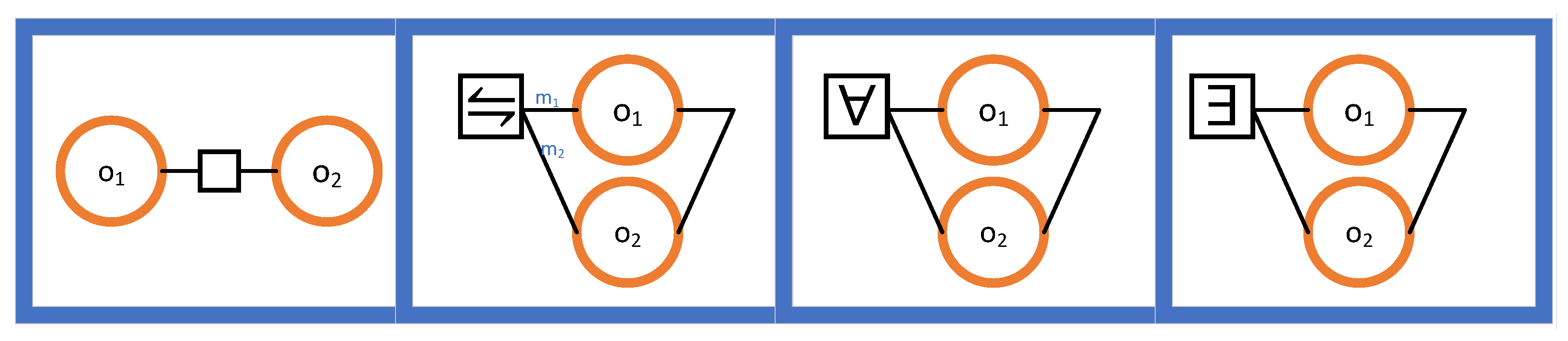
3.2. Outcome Diagrams and Outcome Expressions
- In the first case, the outcomes and are said to be sequentially composed. Therefore, causally depends on . We maintain a directional convention to avoid showing directions explicitly: when an edge connects two outcomes, the right one causally depends on the left one. The corresponding outcome expression is “”.
- In the second case, a probabilistic choice is made between and . Notice the weights and . The outcome of the choice is the same as with probability and the same as with probability . The corresponding outcome expression is “”.
- In the third case, an all-to-finish (i.e., last-to-finish) combination is produced from and . For two outcomes and that are started at the same time and that are run in parallel, the outcome is done when both and are done. The corresponding outcome expression is “”.
- In the final case, a first-to-finish combination is produced from and . For two outcomes and that are started at the same time and that are run in parallel, the outcome is done when either or is done. The corresponding outcome expression is “”.
3.3. Quality Attenuation ()
3.4. Simple Example
3.5. Alternatives to Outcome Diagrams—Why a New Diagram?
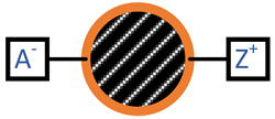
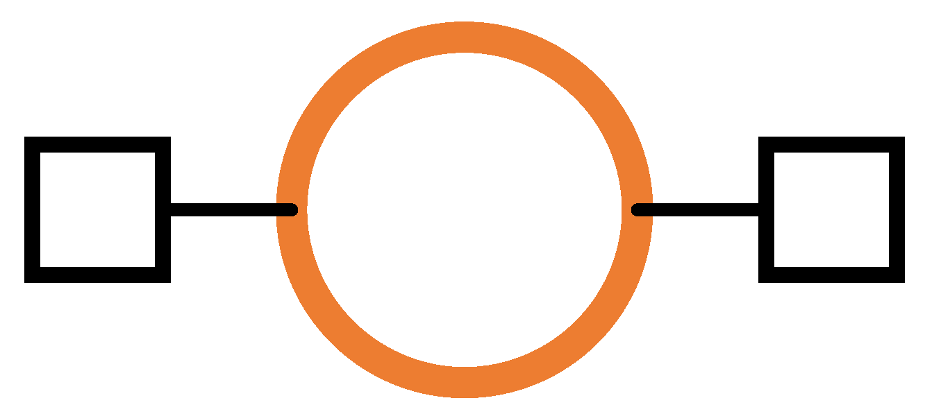
- An outcome diagram specifies the causal relations between outcomes. An outcome is a specific system behaviour defined by its possible starting events and its possible terminating events. For example, sending a message to a server is an outcome defined by the beginning of the send operation and the end of the send operation. The action of sending a message and receiving a reply is observed as an outcome, which is defined by the beginning of the send operation and the end of the receive operation. Outcomes can be decomposed into smaller outcomes, and outcomes can be causally related. For example, the send–receive outcome can be seen as a causal sequence of a send outcome and a receive outcome.
- An outcome diagram can be defined for a partially specified system. Such an outcome diagram can contain undefined outcomes, which are called black boxes. A black box does not correspond to any defined part of the system, but it still has timeliness and resource constraints. Refining an outcome diagram can consist in replacing one of its black boxes with a subgraph of outcomes.
3.5.1. UML Diagrams
- Observational property: All UML diagrams, structural and behavioural, define what happens inside the system being modelled, whereas outcome diagrams define observations from outside the system. The outcome diagram makes no assumptions about the system’s components or internal states.
- Wide coverage property: It is possible for both UML diagrams and outcome diagrams to give partial information about a system, so that they correspond to many possible systems. As long as the systems are consistent with the information in the diagram, they will have the same diagram. However, an outcome diagram corresponds to a much larger set of possible systems than a UML diagram. For an outcome diagram, a system corresponds if it has the same outcomes, independent of its internal structure or behaviour. For a UML diagram, a system corresponds if its internal structure or behaviour is consistent with the information in the diagram. This means that a UML diagram is already making decisions w.r.t. the possible system structures quite early in the design process. The outcome diagram does not make such decisions.
3.5.2. State Machine Diagram
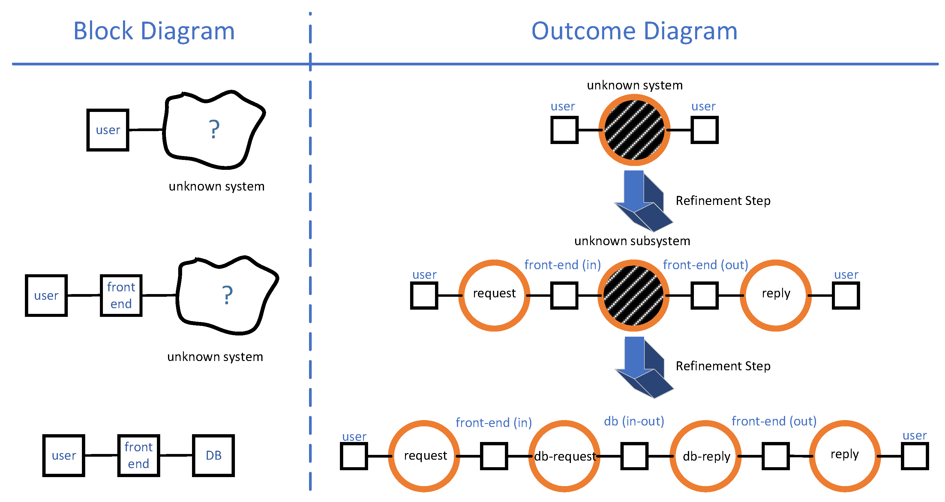
3.5.3. Block Diagram
4. Design Exploration Using Outcome Diagrams
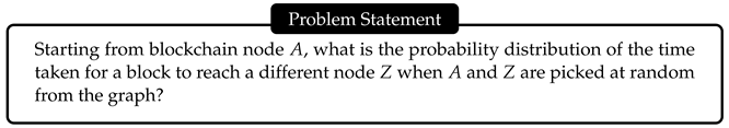
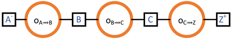
4.1. Starting Off
- : Block is ready to be transmitted by A.
- : Block is received and verified by Z.
4.2. Early Analysis
- The size of the block;
- The speed of the network interface;
- The geographical distance of the hop (as measured by the time to deliver a single packet);
- Congestion along the network path.
- Short: The two nodes are located in the same data centre;
- Medium: The two nodes are located in the same continent;
- Long: The two nodes are located in different continents.
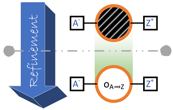
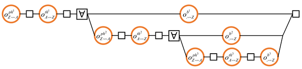
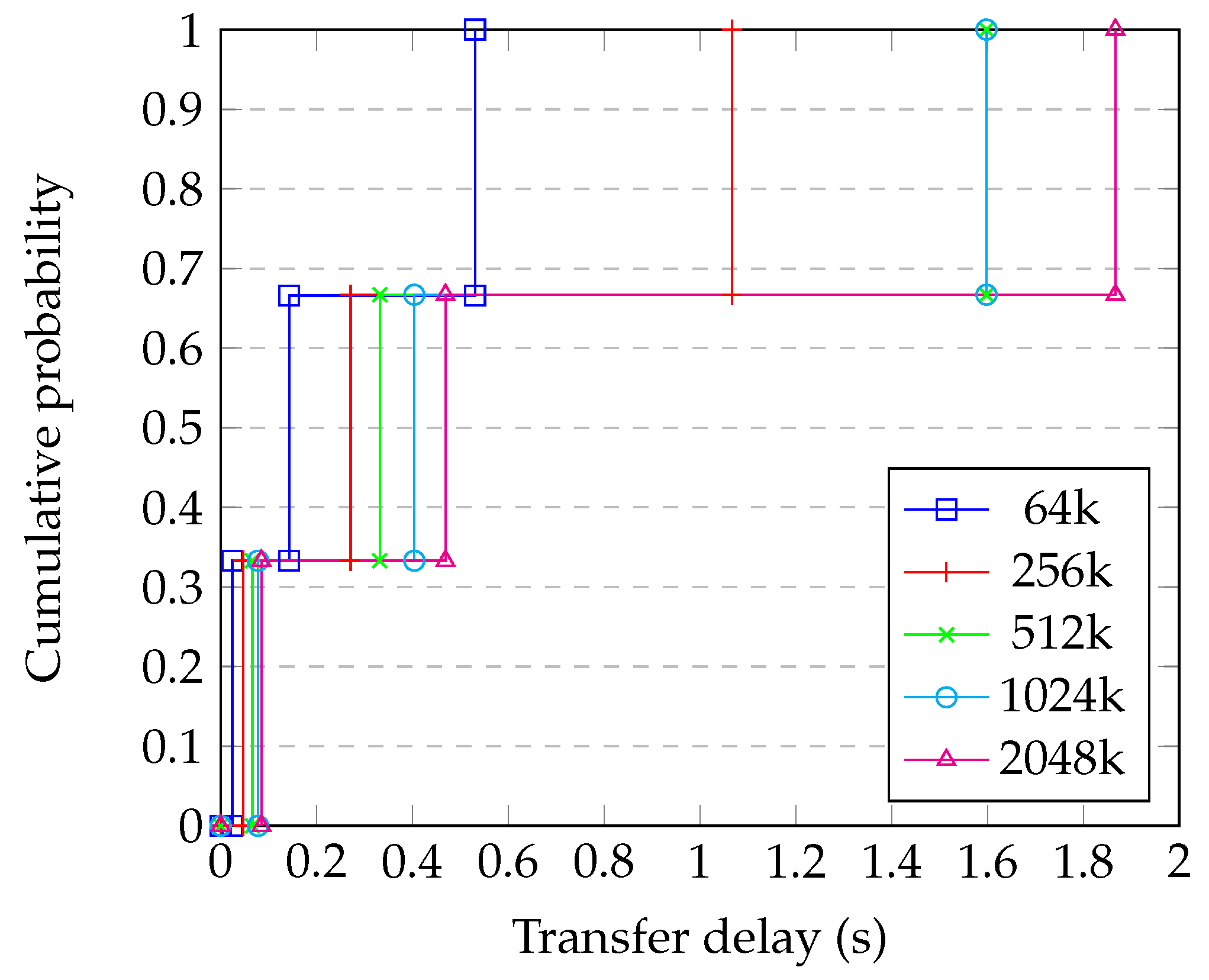
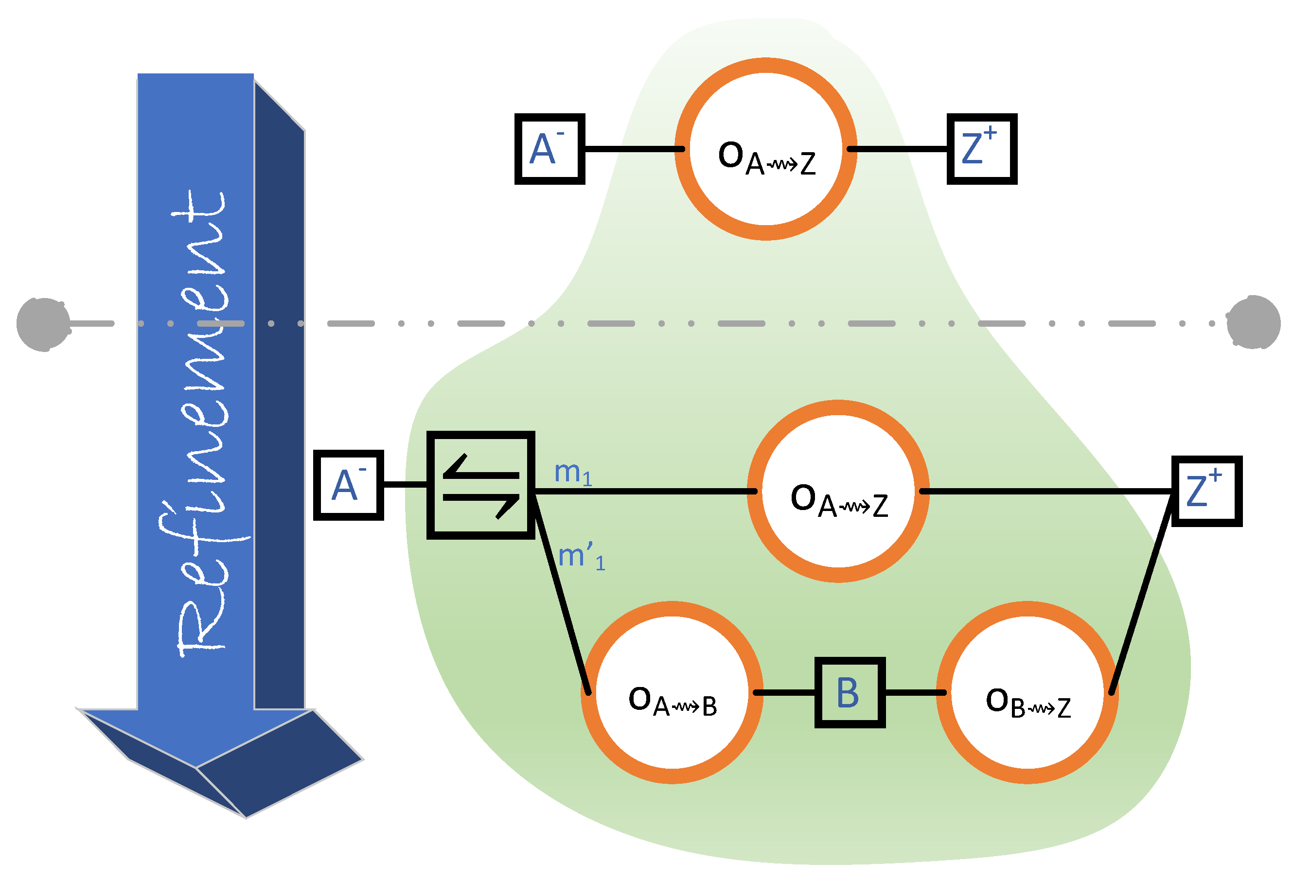
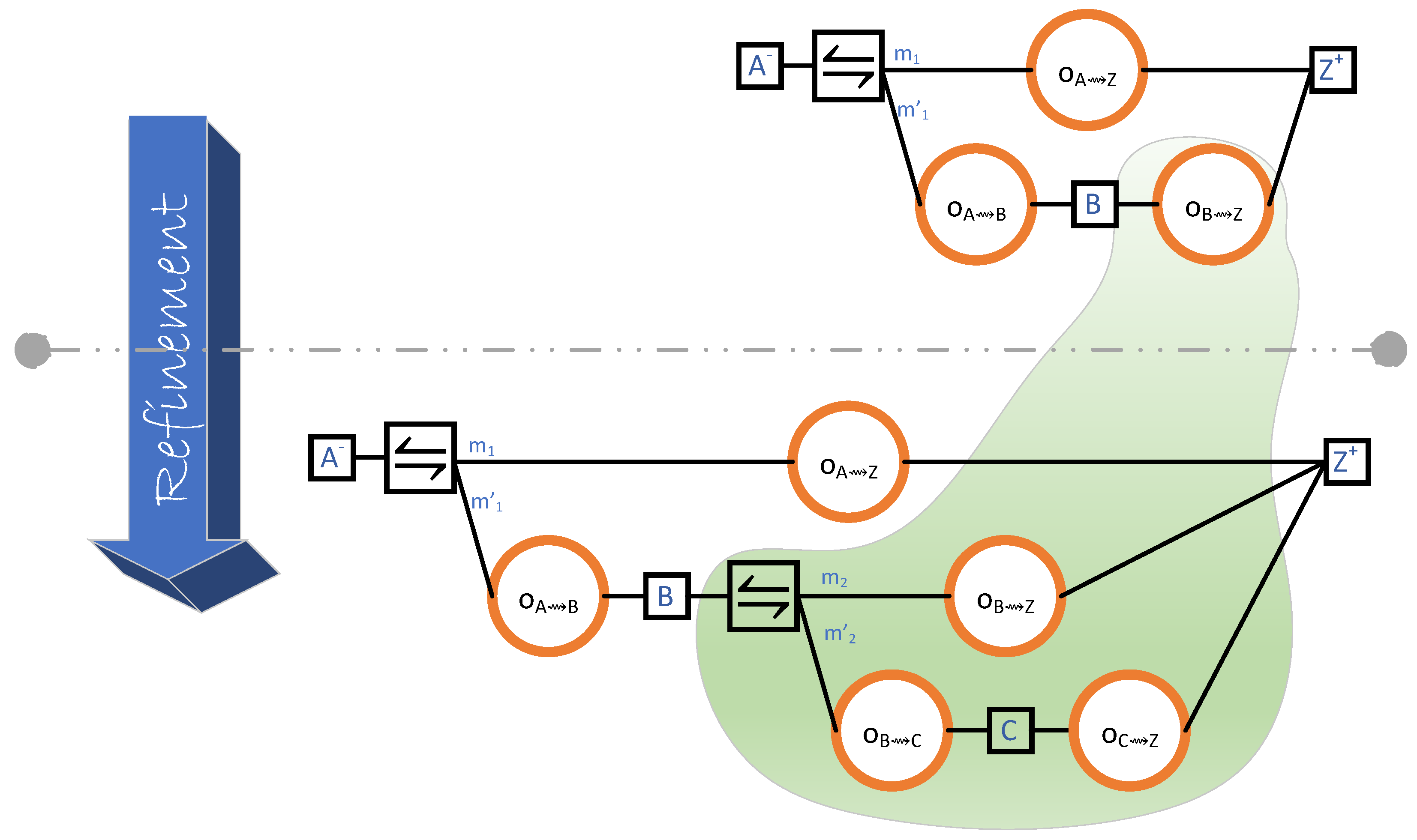
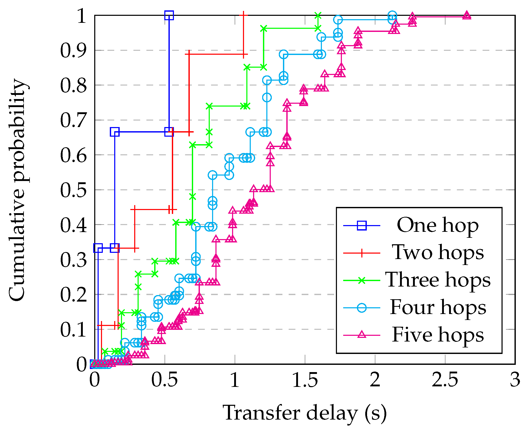
4.3. Refinement and Probabilistic Choice
Alternative Refinements
4.4. Breaking Down Transmissions into Smaller Units
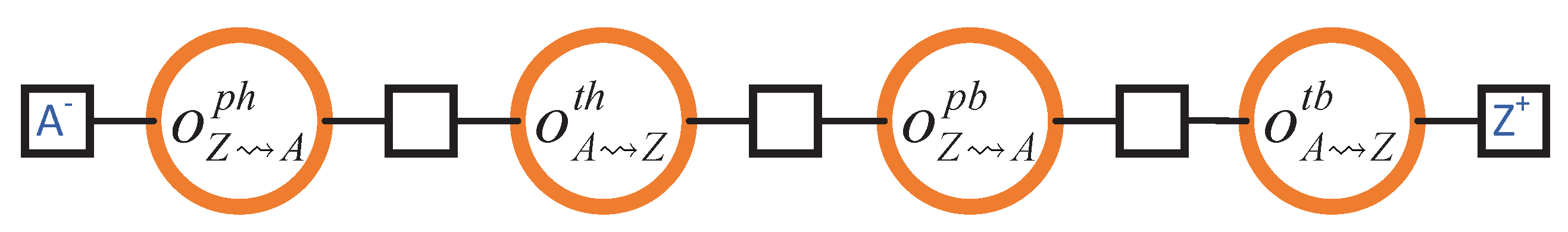
4.5. Header–Body Split
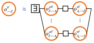
- Permission for Header Transmission (): Node Z grants the permission to node A to send it a header.
- Transmission of the Header (): Node A sends a header to node Z.
- Permission to for Body Transmission (): Node Z analyses the header that was previously sent to it by A. Once the suitability of the block is determined via the header, node Z grants permission to A to send it the respective body of the previously sent header.
- Transmission of the Body (): Finally, A sends the block body to Z.
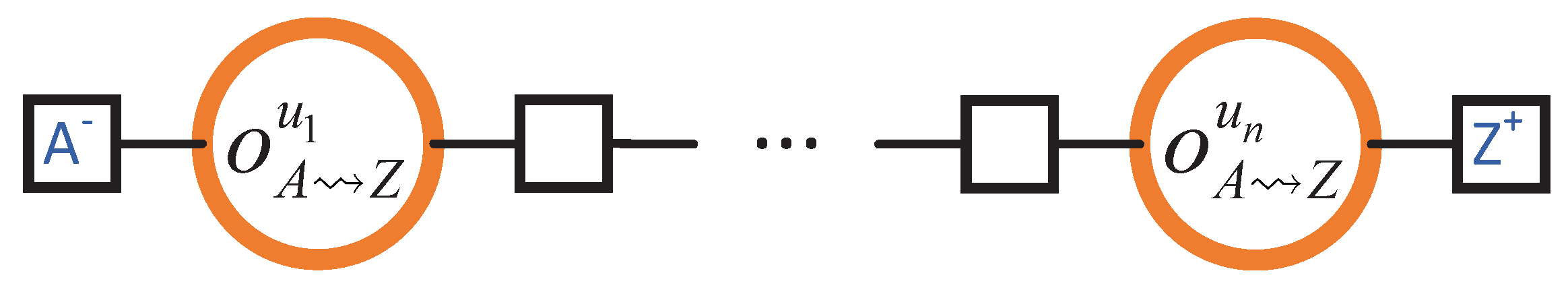
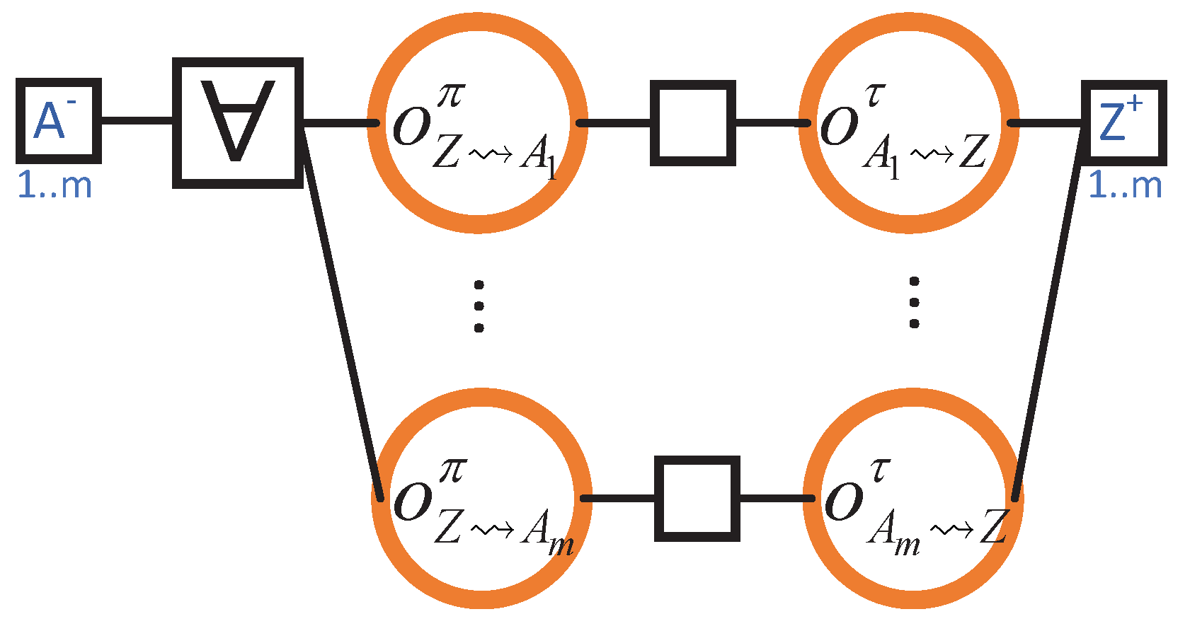
4.6. Obtaining One Block from each Neighbour when Rejoining the Blockchain
- Upon its return to the blockchain, Z is m blocks behind, where m is less than or equal to the number of Z’s neighbours.
- Each neighbour of Z transmits precisely one block to Z.
- The header–body split refinement of Section 4.5 is not considered. Therefore, there are only two steps (instead of the actual four):
- for when Z grants permission to . And,
- for when transmits the (entire) block to Z.
Load Analysis
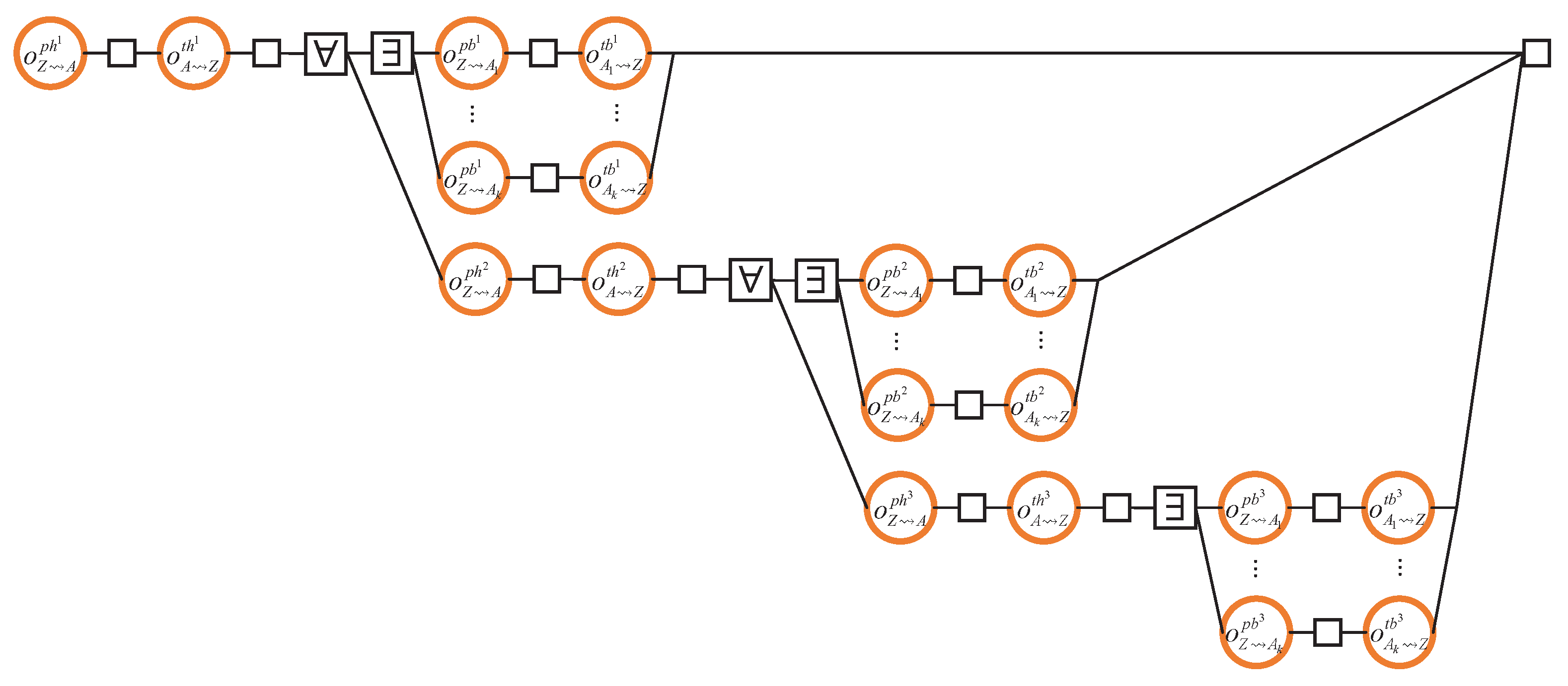
4.7. Obtaining a Block from the Fastest Neighbour
- CO1.
- For each block, the header must be transmitted before the body (so that the recipient node can determine the suitability of the block before the body transmission);
- CO2.
- Headers of the older blocks need to be transmitted before those of the younger blocks (note, however, that there is no causal relationship between the body transmissions).
4.8. Summary
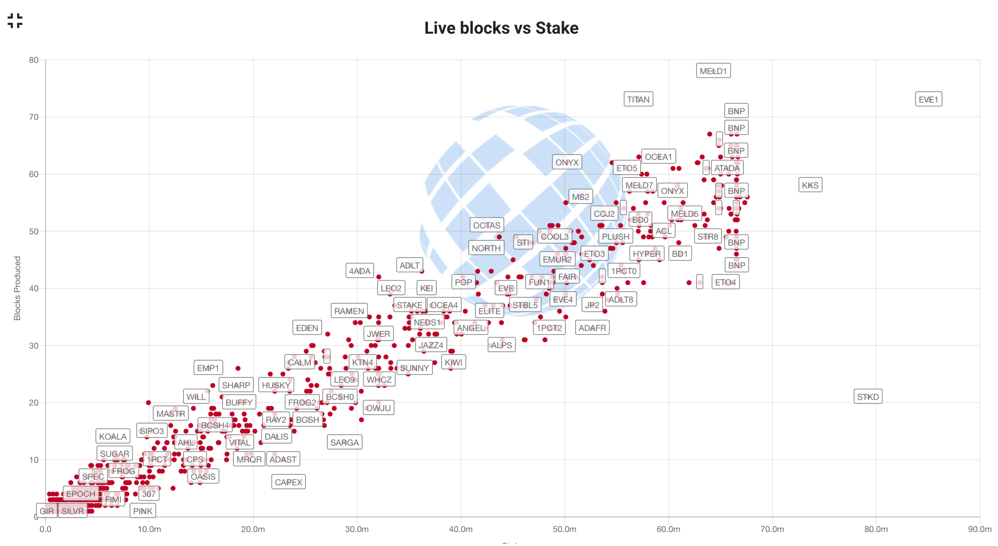
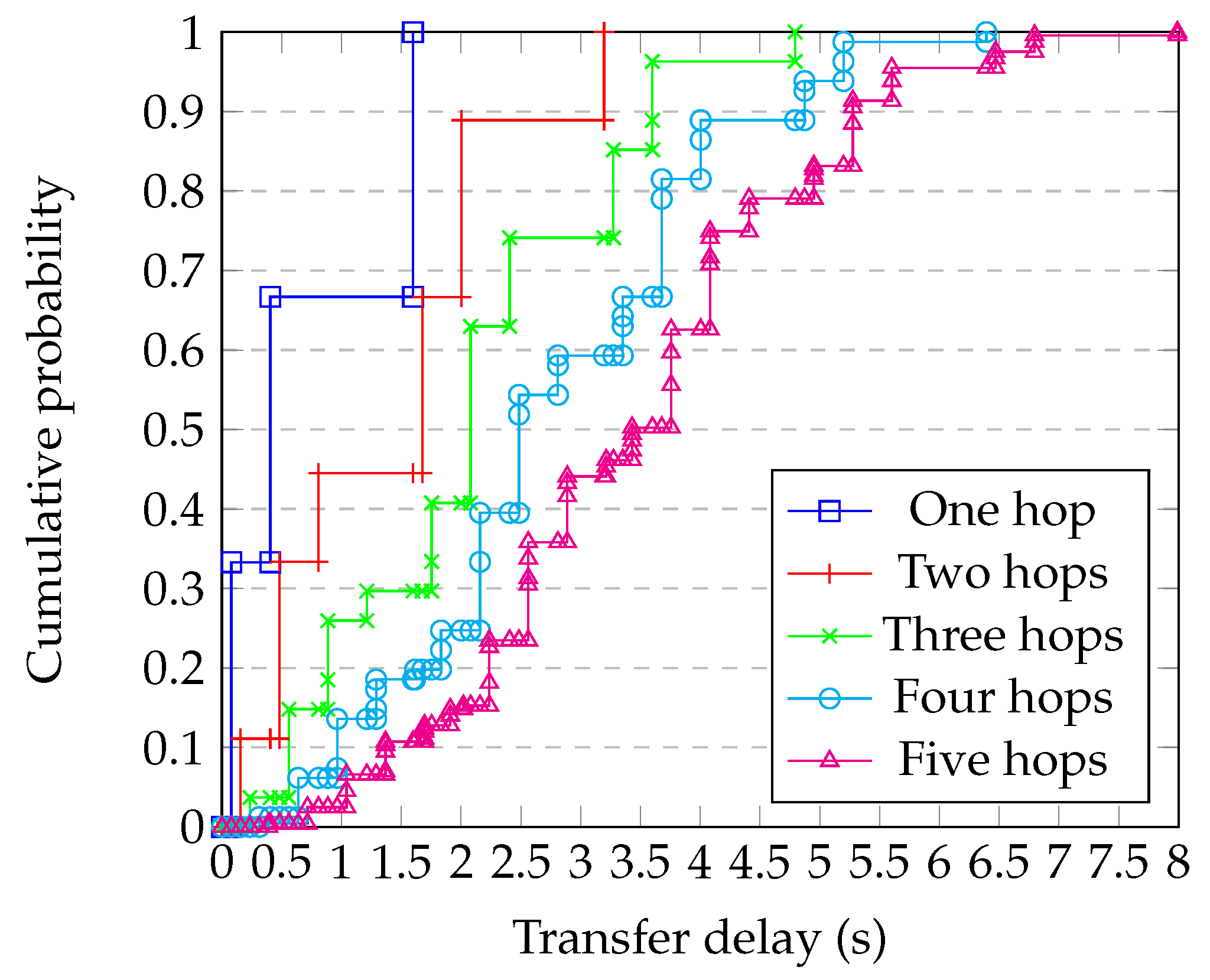
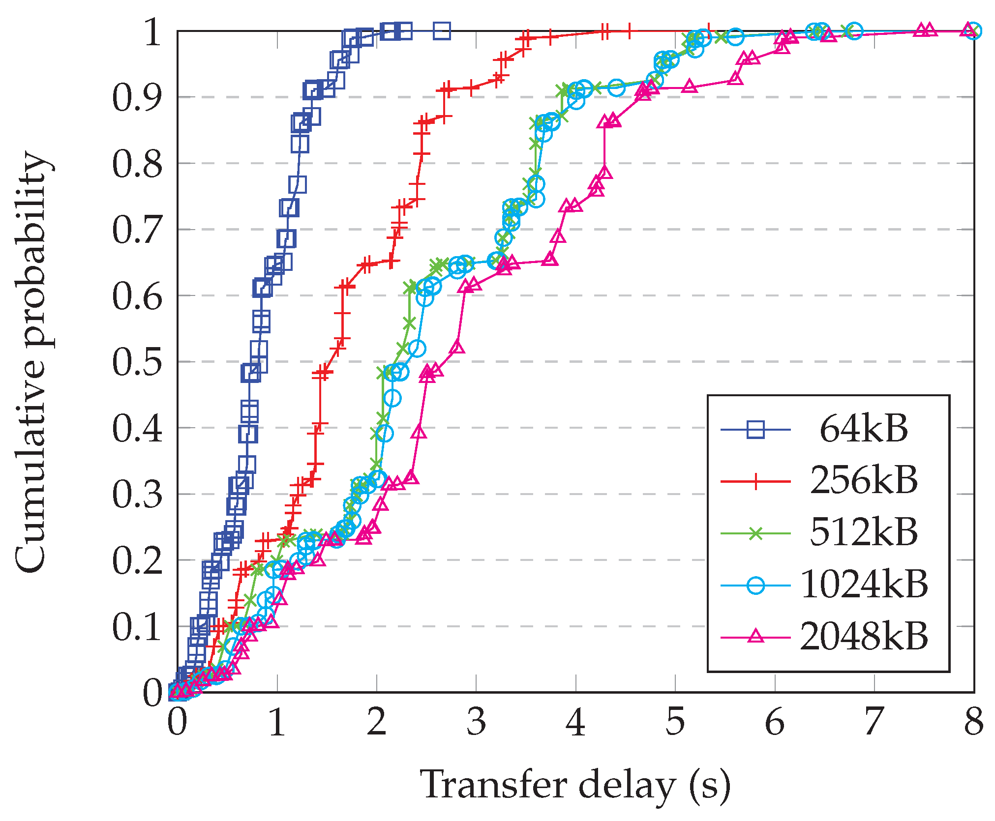
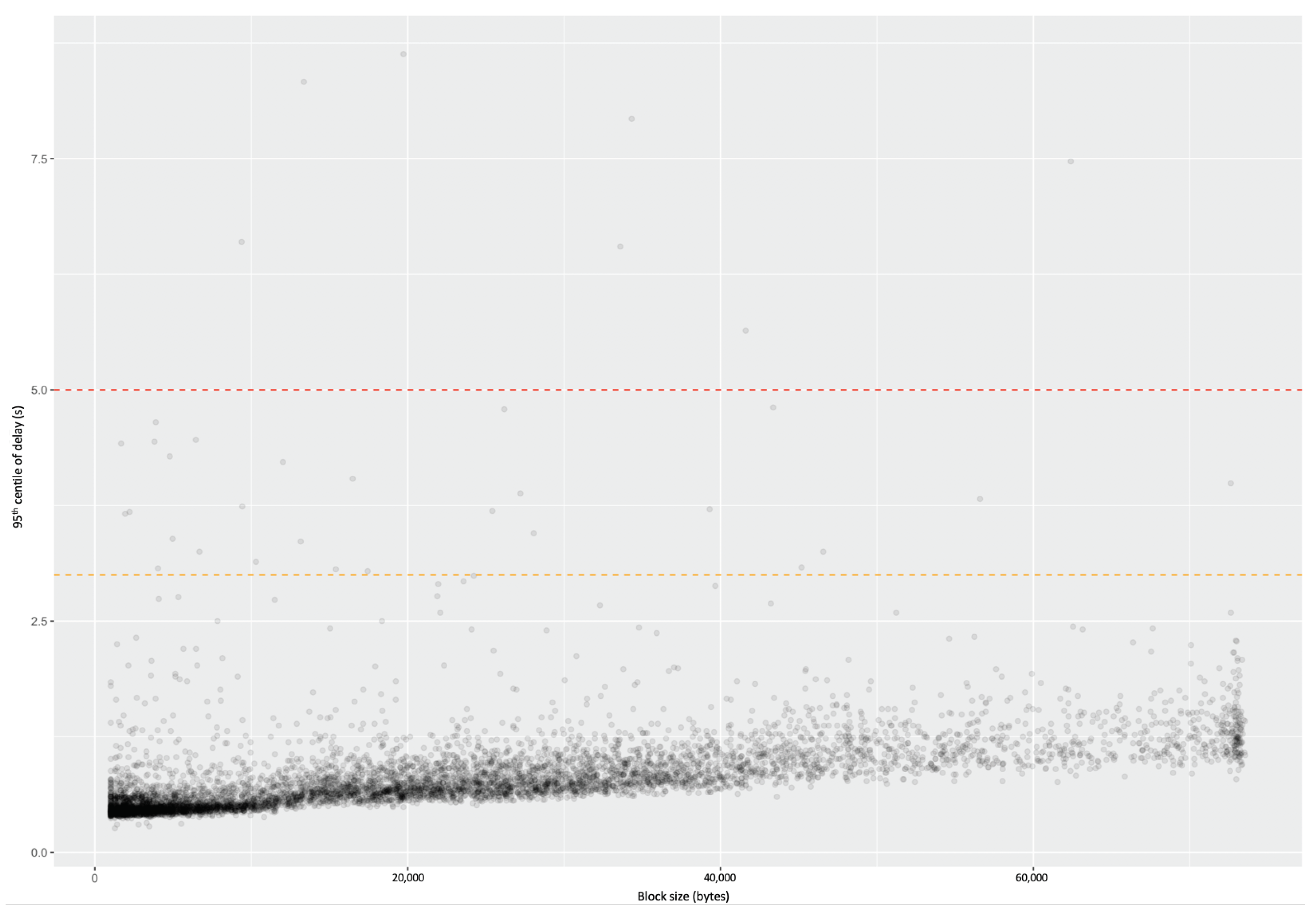
4.9. Comparison with Simulation
- Generating a random graph with 2500 nodes having degree 10;
- Randomly choosing whether each link is ‘short’, ‘medium’, or ‘long’, and applying the corresponding delay from Table 1;
- Running the simulation of the whole system for enough steps to obtain statistical confidence;
- Repeating for each block size;
- Repeating this for enough different graphs to have confidence in the results.
5. A Formalisation of SD
5.1. Notational Conventions
5.2. Syntax
- ♭ in Section 4.1.
- and throughout Section 4.
- in Section 4.3.
- in Section 4.6 and Section 4.7.
- in Section 4.7.
5.3. Timeliness Analysis
- ;
- .
5.4. Load Analysis
6. Related Work
6.1. Alternative Theoretical Approaches
6.1.1. Queuing Theory
6.1.2. Extending Existing Modelling Approaches
6.1.3. Real-Time Systems and Worst-Case Execution Time
6.2. Block Propagation
6.3. Distributed System Design
6.3.1. Iterative Design
6.3.2. Role of the SD Paradigm in Distributed System Design
6.4. Programming Languages and Software Engineering
6.4.1. Programming Paradigms
6.4.2. Software Development Paradigms
- Design-by-Contract. [37] Similarly to SD, in this paradigm, the programmer begins by coding by describing the pre-conditions and the post-condition. Over the years, the concept of refining initial designs from specification to code has gained increasing weight [38]. However, unlike SD, the focus is on functional correctness rather than performance.
- Software Product Lines. [39] This paradigm targets families of software systems that are closely related and that clearly share a standalone base. The aim is to reuse the development effort of and the code for the base across all the different variations in the family. The similarity with SD is that this approach also allows variation in the implementation so long as the required quality constraints are met. In other words, variations can share a given expected outcome and its quality bounds.
- Component-Based Software Engineering. [40] Components, in this paradigm, are identified by their so-called ‘requires’ and ‘provides’ interfaces. That is, so long as two components have the same ‘requires’ and ‘provides’ interfaces, they are deemed equivalent in this paradigm, and they can be used interchangeably. In SD, subsystems can also have quality contracts that involve quantitative ‘demand’ and ‘supply’ specifications. Such contracts impose quality restrictions (say, timeliness or pattern of consumption) on the respective outcomes of those subsystems. However, we have not shown examples of quality contracts in this paper, because their formalisation is not yet complete.
6.4.3. Algebraic Specification and Refinement
6.4.4. Amortised Analysis
7. Conclusions
7.1. Takeaways for System Designers
7.1.1. Outcome Diagrams
7.1.2. Design Example
7.1.3. Recommendations
7.2. Limitations of the SD Paradigm
- Contextuality vs. Compositionality:As a performance modelling tool, SD deliberately trades detail in exchange for compositionality. The highest level of detail is provided by timed traces of a real system or a discrete event simulation thereof. A level of abstraction is provided by the use of generator functions [49], which obscure some details such as data-dependency but retain the local temporal context. Representing behaviour using random variables removes the temporal context, treating aspects of the system as Markovian. Thus, the SD paradigm is most applicable to systems that execute many independent instances of the same action, such as diffusing blocks, streaming video frames, or responding to web requests. For systems that engage in long sequences of highly dependent actions, it may only deliver bounding estimates.
- Non-linearity: In many systems, resource sharing may introduce a relationship between load and , which can be incorporated in to the analysis. An obvious example is a simple queue (which is ubiquitous in networks), where the delay/loss is a function of the applied load. However, where system behaviour introduces a further relationship between and load, for example due to timeouts and retries, the coupling becomes non-linear. In this case, a satisfactory performance analysis requires iterating to a fixed point, which may not be forthcoming. Failure to find a fixed point can be considered a warning that the performance of the system may be unstable.
7.3. Future Work
Author Contributions
Funding
Institutional Review Board Statement
Informed Consent Statement
Data Availability Statement
Conflicts of Interest
References
- Narcisse, E. What Went Wrong with OnLive? Kotaku.com, G/O Media: New York, NY, USA, 2012. [Google Scholar]
- Wolverton, T. Exclusive: OnLive Assets Were Sold Off for Just $4.8 Million; The Mercury News: San Jose, CA, USA, 2012. [Google Scholar]
- Hollister, S. OnLive Lost: How the Paradise of Streaming Games Was Undone by One Man’s Ego; The Verge, Vox Media: New York, NY, USA, 2012. [Google Scholar]
- Pressman, R.; Maxim, D.B.R. Software Engineering: A Practitioner’s Approach; McGraw-Hill: New York, NY, USA, 2014. [Google Scholar]
- Krasner, H. The Cost of Poor Software Quality in the US: A 2020 Report; Technical Report; CISQ Consortium for Information & Software Quality: Needham, MA, USA, 2020. [Google Scholar]
- Davies, N. Developing Systems with Awareness of Performance. In Proceedings of Workshop on Process Algebra and Performance Modelling; CSR-26-93; Department of Computer Science, University of Edinburgh: Edinburgh, UK, 1993; pp. 7–10. [Google Scholar]
- Perry, D.E.; Wolf, A.L. Foundations for the study of software architecture. ACM Sigsoft Softw. Eng. Notes 1992, 17, 40–52. [Google Scholar] [CrossRef]
- Alford, M.W. A requirements engineering methodology for real-time processing requirements. IEEE Trans. Softw. Eng. 1977, 1, 60–69. [Google Scholar] [CrossRef]
- Kant, P.; Hammond, K.; Coutts, D.; Chapman, J.; Clarke, N.; Corduan, J.; Davies, N.; Díaz, J.; Güdemann, M.; Jeltsch, W.; et al. Flexible Formality Practical Experience with Agile Formal Methods. In Trends in Functional Programming; Byrski, A., Hughes, J., Eds.; Springer International Publishing: Cham, Switzerland, 2020; pp. 94–120. [Google Scholar]
- Solutions, P.N. Assessment of Traffic Management Detection Methods and Tools; Technical Report MC-316; Ofcom: London, UK, 2015. [Google Scholar]
- Thompson, P.; Davies, N. Towards a RINA-Based Architecture for Performance Management of Large-Scale Distributed Systems. Computers 2020, 9, 53. [Google Scholar] [CrossRef]
- Drescher, D. Blockchain Basics: A Non-Technical Introduction in 25 Steps; Apress: Frankfurt am Main, Germany, 2017. [Google Scholar]
- David, B.; Gaži, P.; Kiayias, A.; Russell, A. Ouroboros Praos: An Adaptively-Secure, Semi-synchronous Proof-of-Stake Blockchain. In Advances in Cryptology—EUROCRYPT 2018; Nielsen, J.B., Rijmen, V., Eds.; Springer International Publishing: Cham, Switzerland, 2018; pp. 66–98. [Google Scholar]
- Coutts, D.; Davies, N.; Szamotulski, M.; Thompson, P. Introduction to the Design of the Data Diffusion and Networking for Cardano Shelley; Technical Report; IOHK: Singapore, 2020. [Google Scholar]
- Watts, D.J. Small Worlds: The Dynamics of Networks between Order and Randomness; Princeton University Press: Princeton, NJ, USA, 2003; p. 280. [Google Scholar]
- Leon Gaixas, S.; Perello, J.; Careglio, D.; Gras, E.; Tarzan, M.; Davies, N.; Thompson, P. Assuring QoS Guarantees for Heterogeneous Services in RINA Networks with ΔQ. In Proceedings of the IEEE International Conference on Cloud Computing Technology and Science (CloudCom), Luxembourg City, Luxembourg, 12–15 December 2016; pp. 584–589. [Google Scholar]
- Trivedi, K.S. Probability and Statistics with Reliability, Queuing, and Computer Science Applications, 2nd ed.; Wiley: New York, NY, USA, 2002. [Google Scholar]
- Voulgaris, S.; (Institute of Information and Communication Technologies, Université catholique de Louvain, Louvain-la-Neuve, Belgium). Private Communication, 2021.
- McKay, B.D. Enumeration and Design; Academic Press: Cambridge, MA, USA, 1984; Volume A19, pp. 225–238. [Google Scholar]
- Reiser, M.; Lavenberg, S.S. Mean-value analysis of closed multichain queuing networks. J. ACM 1980, 27, 313–322. [Google Scholar] [CrossRef]
- Jackson, J.R. Jobshop-like queueing systems. Manag. Sci. 1963, 10, 131–142. [Google Scholar] [CrossRef]
- Molloy, M.K. Performance analysis using stochastic petri nets. IEEE Trans. Comput. 1982, 31, 913–917. [Google Scholar] [CrossRef]
- Moller, F.; Tofts, C. A Temporal Calculus for Communicating Systems. In Proceedings of the CONCUR ’90 Theories of Concurrency: Unification and Extension, Amsterdam, The Netherlands, 27–30 August 1990; Springer: Berlin/Heidelberg, Germany, 1989; Volume 458, pp. 401–415. [Google Scholar]
- Jou, C.C.; Smolka, S.A. Equivalences, Congruences and Complete Axiomatizations of Probabilistic Processes. In Proceedings of the CONCUR ’90 Theories of Concurrency: Unification and Extension, Amsterdam, The Netherlands, 27–30 August 1990; Springer: Berlin/Heidelberg, Germany, 1989; Volume 458, pp. 367–383. [Google Scholar]
- Hillston, J. A Compositional Approach to Performance Modelling; Cambridge University Press: Cambridge, UK, 1996. [Google Scholar]
- Bradley, J.T.; Dingle, N.J.; Gilmore, S.T.; Knottenbelt, W.J. Derivation of passage-time densities in PEPA models using IPC: The Imperial PEPA Compiler. In Proceedings of the 11th IEEE/ACM International Symposium on Modeling, Analysis and Simulation of Computer Telecommunications Systems, Orlando, FL, USA, 12–15 October 2003. [Google Scholar]
- Daduna, H. Burke’s Theorem on Passage Times in Gordon-Newell Networks. Adv. Appl. Probab. 1984, 16, 867–886. [Google Scholar] [CrossRef]
- Hsu, G.-H.; Yuan, X.-M. First passage times and their algorithms for markov processes. Commun. Stat. Stoch. Model. 1995, 11, 195–210. [Google Scholar] [CrossRef]
- Bradley, J.; Davies, N. Performance Modelling and Synchronisation; Working Paper: CSTR-98-009, Superseded by CSTR-99-002; University of Bristol: Bristol, UK, 1998. [Google Scholar]
- Chatrabgoun, O.; Daneshkhah, A.; Parham, G. On the functional central limit theorem for first passage time of nonlinear semi-Markov reward processes. Commun. Stat.-Theory Methods 2020, 49, 4737–4750. [Google Scholar] [CrossRef]
- Wilhelm, R.; Engblom, J.; Ermedahl, A.; Holsti, N.; Thesing, S.; Whalley, D.; Bernat, G.; Ferdinand, C.; Heckmann, R.; Mitra, T.; et al. The Worst-Case Execution-Time Problem—Overview of Methods and Survey of Tools. ACM Trans. Embed. Comput. Syst. 2008, 7, 36. [Google Scholar] [CrossRef]
- Decker, C.; Wattenhofer, R. Information propagation in the Bitcoin network. In Proceedings of the IEEE P2P 2013 Proceedings, Trento, Italy, 9–11 September2013; pp. 1–10. [Google Scholar] [CrossRef]
- Croman, K.; Decker, C.; Eyal, I.; Gencer, A.E.; Juels, A.; Kosba, A.; Miller, A.; Saxena, P.; Shi, E.; Gün Sirer, E.; et al. On Scaling Decentralized Blockchains; Financial Cryptography and Data Security; Clark, J., Meiklejohn, S., Ryan, P.Y., Wallach, D., Brenner, M., Rohloff, K., Eds.; Springer: Berlin/Heidelberg, Germany, 2016; pp. 106–125. [Google Scholar]
- Shahsavari, Y.; Zhang, K.; Talhi, C. A Theoretical Model for Block Propagation Analysis in Bitcoin Network. IEEE Trans. Eng. Manag. 2020, 1–18. [Google Scholar] [CrossRef]
- Dotan, M.; Pignolet, Y.A.; Schmid, S.; Tochner, S.; Zohar, A. Survey on Blockchain Networking: Context, State-of-the-Art, Challenges. ACM Comput. Surv. 2021, 54, 107. [Google Scholar] [CrossRef]
- Gibbons, J. (Ed.) Generic and Indexed Programming. In Proceedings of the International Spring School, SSGIP 2010, Oxford, UK, 22–26 March 2010. [Google Scholar] [CrossRef]
- Meyer, B. Applying “Design by Contract”. Computer 1992, 25, 40–51. [Google Scholar] [CrossRef] [Green Version]
- Weigand, H.; Dignum, V.; Meyer, J.J.C.; Dignum, F. Specification by Refinement and Agreement: Designing Agent Interaction Using Landmarks and Contracts. In Proceedings of the Third International Workshop, ESAW 2002, Madrid, Spain, 16–17 September 2002. [Google Scholar] [CrossRef] [Green Version]
- Apel, S.; Batory, D.B.; Kästner, C.; Saake, G. Feature-Oriented Software Product Lines—Concepts and Implementation; Springer: Berlin/Heidelberg, Germany, 2013. [Google Scholar] [CrossRef]
- Pree, W. Component-Based Software Development—A New Paradigm in Software Engineering? Softw. Concepts Tools 1997, 18, 169–174. [Google Scholar]
- Baumeister, H. Relating Abstract Datatypes and Z-Schemata. In Proceedings of the 14th International Workshop, WADT’99, Château de Bonas, France, 15–18 September 1999. [Google Scholar]
- Kahrs, S.; Sannella, D.; Tarlecki, A. The Definition of Extended ML: A Gentle Introduction. Theor. Comput. Sci. 1997, 173, 445–484. [Google Scholar] [CrossRef] [Green Version]
- Haveraaen, M. Institutions, Property-Aware Programming and Testing. In Proceedings of the LCSD’07: Proceedings of the 2007 Symposium on Library-Centric Software Design, Montreal, BC, Canada, 21 October 2007; ACM: New York, NY, USA, 2007; pp. 21–30. [Google Scholar] [CrossRef]
- Astesiano, E.; Bidoit, M.; Kirchner, H.; Krieg-Brückner, B.; Mosses, P.D.; Sannella, D.; Tarlecki, A. Casl: The Common Algebraic Specification Language. Theor. Comput. Sci. 2002, 286, 153–196. [Google Scholar] [CrossRef] [Green Version]
- Simões, H.R.; Vasconcelos, P.B.; Florido, M.; Jost, S.; Hammond, K. Automatic amortised analysis of dynamic memory allocation for lazy functional programs. In Proceedings of the ACM SIGPLAN International Conference on Functional Programming, ICFP’12, Copenhagen, Denmark, 9–15 September 2012; ACM: New York, NY, USA, 2012; pp. 165–176. [Google Scholar] [CrossRef]
- Jost, S.; Vasconcelos, P.B.; Florido, M.; Hammond, K. Type-Based Cost Analysis for Lazy Functional Languages. J. Autom. Reason. 2017, 59, 87–120. [Google Scholar] [CrossRef] [Green Version]
- Rajani, V.; Gaboardi, M.; Garg, D.; Hoffmann, J. A unifying type-theory for higher-order (amortized) cost analysis. Proc. ACM Program. Lang. 2021, 5, 1–28. [Google Scholar] [CrossRef]
- Adams, D. The Hitchhiker’s Guide to the Galaxy; Harmony Books: London, UK, 1979. [Google Scholar]
- Reilly, E.D.; Ralston, A.; Hemmendinger, D. Encyclopedia of Computer Science; Nature Pub. Group: London, UK, 2000. [Google Scholar]
- Van Roy, P.; Davies, N.; Thompson, P.; Haeri, S.H. The ΔQSD Systems Development Paradigm, a Tutorial. In Proceedings of the HiPEAC Conference (High-Performance Embedded Architecture and Compilation), Budapest, Hungary, 20–22 June 2022. [Google Scholar]
- Thompson, P.; Hernadaz, R. Quality Attenuation Measurement Architecture and Requirements; Technical Report TR-452.1; Broadband Forum: Fremont, CA, USA, 2020. [Google Scholar]


| 64 kB | 256 kB | 512 kB | 1024 kB | 2048 kB | |||||||
|---|---|---|---|---|---|---|---|---|---|---|---|
| Distance | Time (s) | Time (s) | RTTs | Time (s) | RTTs | Time (s) | RTTs | Time (s) | RTTs | Time (s) | RTTs |
| Short | 0.012 | 0.024 | 1.95 | 0.047 | 3.81 | 0.066 | 5.41 | 0.078 | 6.36 | 0.085 | 6.98 |
| Medium | 0.069 | 0.143 | 2.07 | 0.271 | 3.94 | 0.332 | 4.82 | 0.404 | 5.87 | 0.469 | 6.81 |
| Long | 0.268 | 0.531 | 1.98 | 1.067 | 3.98 | 1.598 | 5.96 | 1.598 | 5.96 | 1.867 | 6.96 |
| Length | Node Degree | |||
|---|---|---|---|---|
| 5 | 10 | 15 | 20 | |
| 1 | 0.20 | 0.40 | 0.60 | 0.80 |
| 2 | 1.00 | 3.91 | 8.58 | 14.72 |
| 3 | 4.83 | 31.06 | 65.86 | 80.08 |
| 4 | 20.18 | 61.85 | 24.95 | 4.40 |
| 5 | 47.14 | 2.78 | 0.00 | |
| 6 | 24.77 | 0.00 | ||
| 7 | 1.83 | |||
| 8 | 0.05 | |||
| Distance | Block Size (kB) | ||||
|---|---|---|---|---|---|
| 64 | 256 | 512 | 1024 | 2048 | |
| Short | 42.7 | 58.5 | 75.9 | 151.7 | 224.4 |
| Medium | 6.9 | 10.1 | 15.6 | 31.1 | 41.0 |
| Long | 1.9 | 2.6 | 3.1 | 6.2 | 10.2 |
Publisher’s Note: MDPI stays neutral with regard to jurisdictional claims in published maps and institutional affiliations. |
© 2022 by the authors. Licensee MDPI, Basel, Switzerland. This article is an open access article distributed under the terms and conditions of the Creative Commons Attribution (CC BY) license (https://creativecommons.org/licenses/by/4.0/).
Share and Cite
Haeri, S.H.; Thompson, P.; Davies, N.; Van Roy, P.; Hammond, K.; Chapman, J. Mind Your Outcomes: The ΔQSD Paradigm for Quality-Centric Systems Development and Its Application to a Blockchain Case Study. Computers 2022, 11, 45. https://doi.org/10.3390/computers11030045
Haeri SH, Thompson P, Davies N, Van Roy P, Hammond K, Chapman J. Mind Your Outcomes: The ΔQSD Paradigm for Quality-Centric Systems Development and Its Application to a Blockchain Case Study. Computers. 2022; 11(3):45. https://doi.org/10.3390/computers11030045
Chicago/Turabian StyleHaeri, Seyed Hossein, Peter Thompson, Neil Davies, Peter Van Roy, Kevin Hammond, and James Chapman. 2022. "Mind Your Outcomes: The ΔQSD Paradigm for Quality-Centric Systems Development and Its Application to a Blockchain Case Study" Computers 11, no. 3: 45. https://doi.org/10.3390/computers11030045
APA StyleHaeri, S. H., Thompson, P., Davies, N., Van Roy, P., Hammond, K., & Chapman, J. (2022). Mind Your Outcomes: The ΔQSD Paradigm for Quality-Centric Systems Development and Its Application to a Blockchain Case Study. Computers, 11(3), 45. https://doi.org/10.3390/computers11030045