Modeling and Numerical Validation for an Algorithm Based on Cellular Automata to Reduce Noise in Digital Images

Abstract

Given the grid features of digital images, a direct relation with cellular automata can be established with transition rules based on information of the cells in the grid. This document presents the modeling of an algorithm based on cellular automata for digital images processing. Using an adaptation mechanism, the algorithm allows the elimination of impulsive noise in digital images. Additionally, the comparison of the cellular automata algorithm and median and mean filters is carried out to observe that the adaptive process obtains suitable results for eliminating salt and pepper type-noise. Finally, by means of examples, the result of the algorithm are shown graphically.

1. Introduction

The concept of the cellular automata (CA) was first introduced by Stan Ulam and John von Neumann in the 1940s while they were working on the Manhattan Project at Los Alamos National Laboratory [1]. A remarkable contribution to the development of cellular automata raised from the research of Slam in the study of crystal growth and the interest of von Neumann in self-replicating systems [1]. The initial idea was focused on developing a two-dimensional cellular automaton comprising a grid of square cells. Considering the neighboring cells of a certain cell, it can take a black or white state [1]. According to John von Neumann’s approach, for a certain cell, the neighborhood is composed of four adjacent squares, that is, the cellular automaton can be seen as a cross composed of square cells [1,2]. Based on the above, it is stated, in general terms, that an automaton consists of a set of cells delimited by a finite number of states, the neighborhood, and local transition rules [3].

Therefore, cellular automata are considered as discrete dynamic systems of finite spatial and temporal state composed of a finite set of cells that evolve in parallel in discrete time steps [1,4]; in other words, they are discrete in space and time, allowing the description of local interactions employing transition rules for each cell in the space. In this way, cellular automata are structures that can be used for modeling and studying complex non-linear dynamic systems [1,2,5].

Regarding the diversity of applications in which the concept of a cellular automaton is immersed, and with the inherent ease that these present to model systems, researchers and scientists extrapolated the concept of cellular automata to digital images.

Digital images are considered as a two-dimensional representation of a real image from a numerical matrix that records values for each element at a given point. Each position within the matrix is called a pixel, and it takes discrete values according to properties such as brightness (the intensity of light) or color [6].

Regarding characteristics, digital images have some called “basic”. One is the type of image; for example, there are black and white images that only record the intensity of the light that falls on the pixels. Besides, there are non-optical images such as ultrasound or X-rays in which the intensity of sound or X-rays is recorded. Resolution is also a characteristic expressed by the number of pixels per inch (ppi), that is, the higher the resolution, the more detailed the image is. Another is the color depth (of a color image), or “bits per pixel” is the number of bits that describe brightness or color for one pixel. More bits allow recording more shades of gray or more colors. Finally, the image format provides more details on how the numbers are arranged in the image file and includes the type of compression employed [6,7].

Digital image processing arises from the need to improve appearance, and thereby make certain details more evident [8]. As a result, techniques were implemented to treat different image characteristics (brightness, sharpness, contrast, intensity, noise, among others), but particularly, methods that allow the information contained to be highlighted or suppressed selectively in an image [8].

In this sense, one frequently covered defect is noise, since, through different devices capable of capturing digital images, errors or interferences can be generated when transmitting information bits. Theoretically, different types of noise have been defined and classified according to their characteristics. Consequently, treatment methods and techniques have been developed for each one [9].

Conventional techniques include filters in the space and frequency domains (high pass, low pass, average, etc.), which compared to new techniques have shown lower results [10]; for this reason, different alternatives have been developed aiming at getting efficient and visually aesthetic results. Therefore, the combination of methods, techniques, and various mathematical models have been useful to achieve these objectives. Likewise, edge detection plays a relevant role in image processing, since through these algorithms it is possible to identify objects, define patterns, or segment information within images [9].

Regarding a dictionary learning-based approach for image denoising, [11] proposes a scheme to couple MOD (Method of Optimal Directions) and the Approximate K-Singular Value Decomposition (AK-SVD). This approach integrates a reconstruction and learning process into a model to removal multiplicative and additive noise. In this way, a sparse term is used with the purpose of reducing non-Gaussian outliers associated with multiplicative noise. Additionally, a Laplacian Schatten norm is employed to capture the global structure information. Other related work is presented in [12], introducing an approach on a discriminative ridge regression to supervised classification called Discriminative Ridge Machine (DRM). The focus here is to determine a representative model while defining class discriminations of categorical information. The model is also extended considering other existing models like lasso and group lasso, incorporating discriminative information. For implementation, the authors consider a quadratic model that allows analytical solutions in a closed-form.

According to [13], image denoising can be addressed as an inverse problem where an approach is sparse decomposition over redundant dictionaries. In a sparse representation form, the signals correspond to a linear combination of redundant dictionary atoms. Considering this orientation, in [13] is presented an algorithm for image denoising based on Non Negative Matrix Factorization (N-NMF), and sparse representation over redundant dictionary. In this proposal, the dictionary is trained, rooted in samples from noised image, and then it searches for the best representation using the Approximate Matching Pursuit (AMP). Another advancement in this orientation is presented in [14], proposing a non-negative matrix factorization method that learns both clustering and local similarity in a suitable form. Such portrayal exposes data’s inherent geometric property. Applying the representation in the kernel space allows boosting the capability of the model to identify nonlinear structures associated to the data.

Regarding applications based on Robust Principal Component Analysis (RPCA), in [15] is exposed the issues task to eliminate both mixed types and heavy noises from Hyperspectral Images (HSI). Authors address such issue proposing a non-convex development in RCPA for denoising application of hyperspectral images. This approach takes the log-determinant rank approximation and the ${\mathcal{L}}_2$, log norm to restrain the sparse properties of column-wise or low-rank for the component matrices. Another related work can be observed in [16] that proposes a RCPA model based on matrix tri-factorization that uses SVDs computation of small matrices. Thus, such an approach diminishes the complexity of RCPA to make it linear and completely scalable.

Regarding cellular automata and image processing, an approach to CA-based image segmentation is the GrowCut algorithm proposed in [17]. Since this is an interactive image segmentation algorithm, the user selects the set of seed pixels that signalizes the sections of interest in the image. Regarding GrowCut algorithm, in [18] is presented a procedure of interactive image segmentation designed to reduce specific image segmentation problems for identifying regions of interest. The feasibility to automatically generate seeds for GrowCut is shown; besides, authors suggest a method to automate seed generation for the segmentation task in heart images. In addition, a conventional GrowCut cellular automaton using chaotic features is enhanced in [19]. This development employs an extended, stochastic neighborhood, where randomly-selected remote neighbors reinforce the conventional local neighbors. The authors state that according to the results, by having small changes in the initial conditions in the process, major changes can be induced in the segmentation result.

Regarding others works, in [20] is proposed an algorithm for determining the optimal outdoor evacuation routes in hills. The system uses web services to obtain geographic information from Google Image. The routes are determined using graph theory with geographic information (latitude, longitude, and elevation), and cellular automata in 3D.

Meanwhile, in [21], cellular automata rules are optimized for edge detection employing Particle Swarm Optimization (PSO). In this work, it is exposed that cellular automata provides fast computation, the optimization rule, and the adaptability to target images. According to authors, the method is tunable in medical images to identify structures such as cardiac cavities.

Considering the integration of cellular automata with other techniques, in [22] is designed an automaton that could be part of a more complex system to make bio-computers that can be used for teachers in multidisciplinary education. Meanwhile, in [23] is considered a Hybrid Cellular Automata (HCA) architecture for modeling the cardiac cell–cell membrane resistance. This work shows that the modeling proposal reproduces important and complex spatio-temporal properties that can be used in future models. Besides, authors show how the GPU-based technology can accelerate the simulation and analysis of these systems. Finally, in [24], random walk theory and lattice gas cellular automata are used to generate a mathematical model for gluing wood particles.

Given the above, researchers and those interested in the subject have implemented methods, algorithms, or various techniques that combine basic theories with cellular automata to image processing and model applications. Although outstanding results have been obtained, the possibility of conducting research in this area to improve digital image processing using cellular automata is observed.

Regarding previous works, reference [25] presents an algorithm based on cellular automata to reduce impulsive noise in digital images. Meanwhile, the papers [26,27] describe the integration of a cellular neural network and an adaptive cellular automaton for the impulsive noise reduction and edge detection in digital images; finally, the document [28] displays a process for digital images edge detection employing cellular automaton.

As it can be observed, there are different approaches to eliminate noise in digital images, the cellular automata being a suitable alternative given the direct relationship between a cellular automaton and a digital image given its representation in the form of matrices. In this way, explorative research can be carried out to include different behaviors of cellular automata for digital image processing.

Proposal Approach and Document Organization

This document aims at displaying the mathematical model for an algorithm based on cellular automata to eliminate noise in digital images. The considered algorithm is implemented in [25,26,27]; however, the mathematical description of the automata dynamics operation for filtering process is not performed, which is the object of study in this paper.

In this way, the contributions of the article are the presentation of the mathematical model of the CA operation considering the description of the adaptation process for the cellular automaton, and the methodology for statistical analysis using synthetic images.

The motivation in this work is that the cellular automata have a very direct relationship with digital images given their structure, then CA behaviors can be included to process images; particularly, an adaptive behavior of CA modifying the neighborhood of the cells is considered. In this context, it is important to describe this type of behavior mathematically, which can serve as a reference for further works.

The document is organized as follows. First, Section 2 introduces the background; Section 3 displays the cellular automata algorithm to eliminate impulsive noise in digital images. Section 3.2 details the model for the algorithm based on cellular automata. Next, Section 4 presents the simulation results to observe the algorithm characteristics. Finally, the discussion and conclusions are presented in Section 5 and Section 6.

2. Background

Within the field of digital image processing, a large number of researchers who over time have sought to optimize different techniques, methods and methodologies that allow to have greater approximations [8,28]. However, despite the fact that many of these advances have had interesting results, in most cases, they lack support for an evaluation in a more objective sense [28].

Under this approach, the development of supports based on scientific elements for any technique developed gives greater validity not only from the visual aspect it can be evaluated, but also from its fundamental perspective.

2.1. Mathematical Modeling

Commonly in the research field, when carrying out approximations to find the solution to a problem, tools like empirical knowledge, experience in the field, and intuition are employed. However, as suggested by Pyt’ev [29], this can generate all kinds of difficulties that limit its progress, consequently, the use of tools of scientific nature and formalized knowledge allow the development to be widely supported and its validity guaranteed.

The construction, understanding and application of mathematical concepts according to Ouvrier-Buffet [30] convert informal experimentation into properly grounded scientific knowledge. Likewise, thanks to the above, it is possible for a researcher to obtain a series of expected results that can be replicated in different environments without compromising the construction.

Additionally, according to Menskii [31], the construction of a model requires three essential steps; the first is observation, where the behavior of a phenomenon is analyzed to identify its relevant characteristics. Later, it advances to the formulation stage, where a postulate is prepared and associated with such behavior; finally, the equation of the model is developed accordingly with the formulation made.

2.2. Noise Elimination

In this research field, approaches are continually being developed using different methods with interesting results, such as Sahin, Uguz and Sahin in [32], who presented an algorithm made up of two components, fuzzy logic and a CA used for the restoration of digital images contaminated by impulsive noise. The algorithm employs a local fuzzy transition rule that assigns a membership value to the corrupt pixel (in the neighborhood) and allocates the next state value as the center pixel value.

On the other hand, Chui and He in [33] designed a filter using statistical values estimated from the differences between pixel intensities compared to the most similar neighbors. This filter allows eliminating impulsive and Gaussian noise; nevertheless, when the noise level is high, the filter performance decreases.

Likewise, Chan, Ho, and Nikolova [34], propose a method divided into two phases: First, a median filter is applied to identify the candidate pixels affected by noise. In the second, the digital image is restored employing a specialized regularization method over the noisy pixels. This method has suitable results; however, when the size of the window increases, the processing resources also increase.

As previously seen, image processing has been approached from many perspectives reflected in different research points. However, the support of mathematical models provides investigative elements, since it allows to analyze the results from quantitative and qualitative perspectives.

3. Algorithm Based on Cellular Automata

Considering [35], cellular automata is a class of discrete dynamic system that allow to model complex systems. The CA is composed of a set of cells with a dimension D, taking 1, 2 or 3. Image processing employs CA in a two-dimensional space [36]. According to [37], a cellular automaton is composed of three parts:

(a)

Cells or lattice.

(b)

Neighborhood or adjacent neighbors.

(c)

Rules for cell transitions.

Regarding the functioning of a cellular automaton, the state of a cell in time $t+1$ is calculated using its current state and the values of its neighbors in time t[38,39]. A D-dimensional cellular automata can be defined as a 4-tuple $A=\{Z^D,S,N,\delta \}$, where:

• $Z^D$: D-dimensional space of integers.
• S: finite set of to the states of A.
• N: finite ordered subset of $Z^D$ that corresponds to the neighborhood of A.
• $\delta$: local rule (transition function) of A.

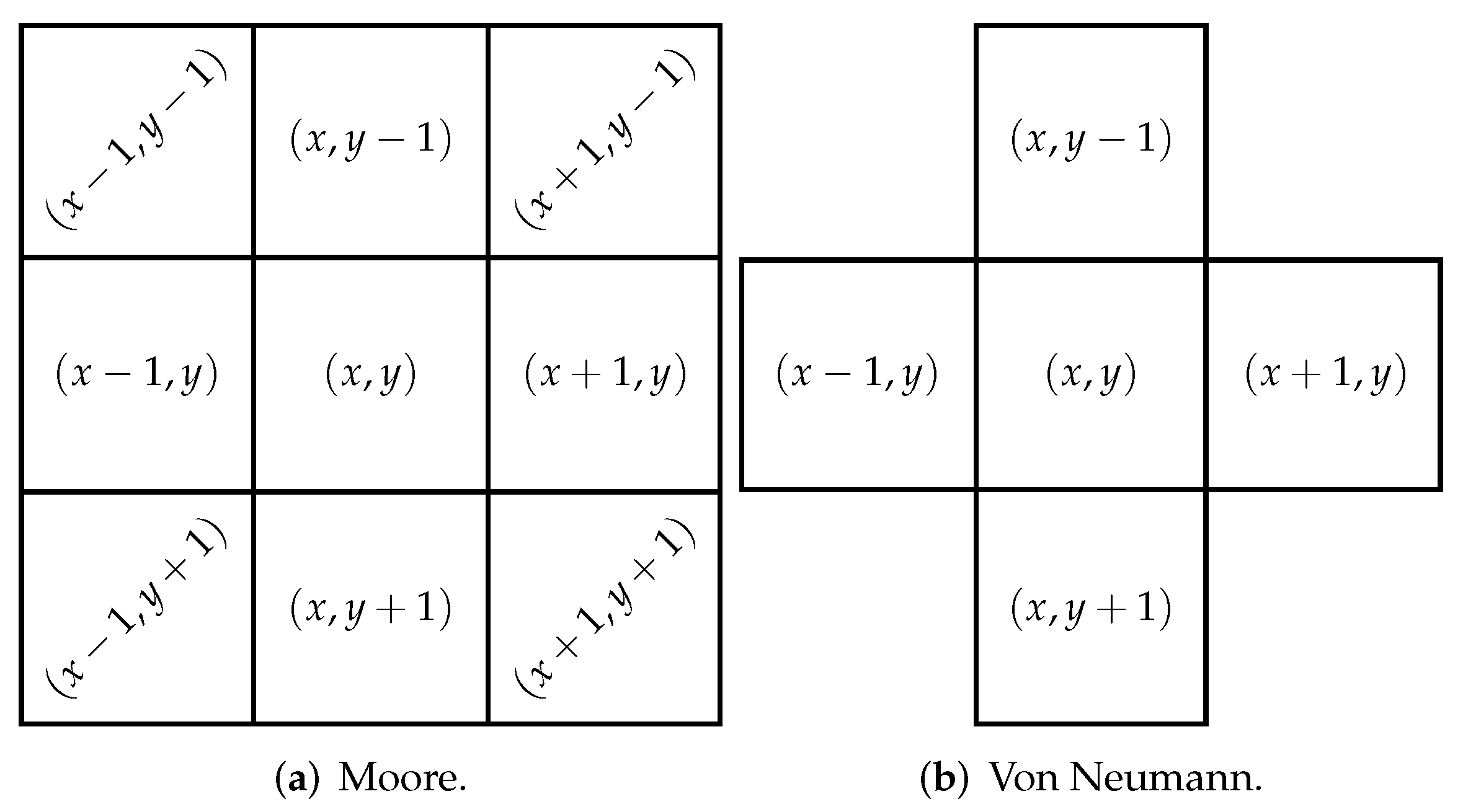
The neighborhood allows us to obtain environmental information. As shown in Figure 1, Moore neighborhood has a configuration of $3\times 3$ matrix that covers a larger number of pixels than the von Neumann neighborhood. The Moore neighborhood is described by Equation (1), where r is the range, for an 8 neighbors $r=1$.

$$N^M(x_0,y_0)=\{(x,y)\in L:|x-x_0|\le r,\mathrm{and}|y-y_0|\le r\}$$

(1)

In order to implement the algorithm, each cell of the CA corresponds to a pixel inside the digital image, where the value of each cell corresponds to an intensity value of the image, in a grayscale image, the values are from 0 to 255 [40]. It is noticeable that the proposed algorithm performs an adaptive modification of the neighborhood where both the first and the last row and column of the image are extended.

3.1. Cellular Automata Algorithm to Eliminate Noise in Digital Images

The mathematical model developed to describe noise elimination in digital images (using CA) is a synthesis of the algorithm presented in [25] called DK (Dynamic-Knowledge), which through the use of cellular automata and an adaptive property, eliminates noise salt and pepper present in a digital grayscale image.

A two-dimensional digital image can be represented as a matrix of size $m\times n$, where each element $a_{i,j}$ found in the i-th row and the j-th column is a pixel within the digital image. The values assigned to the element $a_{i,j}$ corresponds to the luminosity information presented in a pixel [25]. Additionally, a cellular automaton can be defined as a discrete dynamic system composed of a set of cells with a dimension D. The most used to model natural or artificial systems are the two-dimensional ones to easily recreate a collection of simple objects locally interacting with each other [2,3,25].

The DK algorithm uses a Moore neighborhood, which considers 8 neighbors from the base cell (center). Each cell of the cellular automaton can be seen as a pixel within the image, when the algorithm traverses the image using cellular automata and detects a possible noisy pixel, a function is applied to change the pixel value based on the neighbors value. Moreover, when having insufficient information from the neighbor, the cellular automata extends its neighborhood in a row and a column, that is, forming a $5\times 5$ matrix to obtain more data that lead toward the best possible decision.

3.2. Cellular Automata Behavioral Model

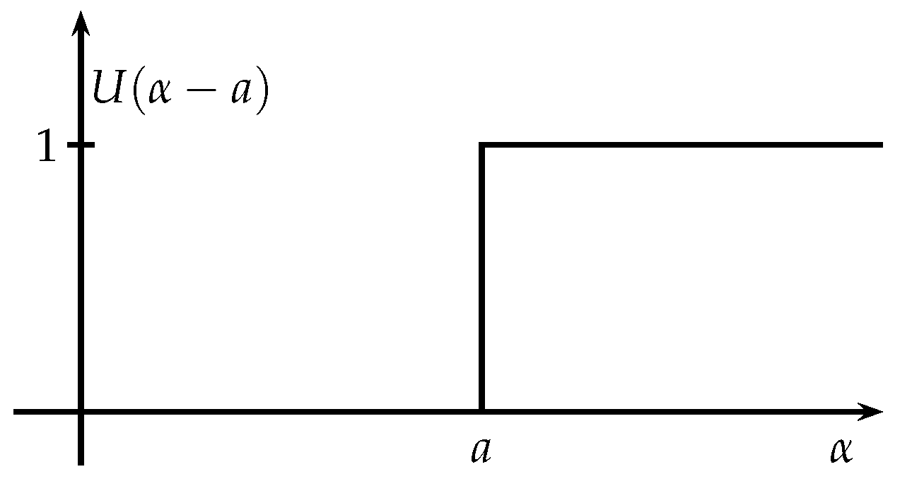
In order to perform the model description, firstly, the unit step function is defined since this is used to activate or deactivate the algorithm adaptive property. In this order is used function $U(\alpha -a)$ given by Equation (2). Figure 2 graphically shows the unitary step function.

$$U(\alpha -a)=\left\{\begin{array}{cc}0,\hfill & if 0\le \alpha <a\hfill \\ 1,\hfill & if \alpha \ge a\hfill \end{array}\right.$$

(2)

Considering a value, function $U(\alpha -a)$ allows describing a piecewise function via turn on/off the components of a function $F\left(\alpha \right)$. For example, $F\left(\alpha \right)$ Equation (3) is represented as $F\left(\alpha \right)=(1-U(\alpha -a))f_1\left(\alpha \right)+U(\alpha -a)f_2\left(\alpha \right)$.

$$F\left(\alpha \right)=\left\{\begin{array}{cc}{f}_1\left(\alpha \right),\hfill & if 0\le \alpha <a\hfill \\ f_2\left(\alpha \right),\hfill & if \alpha \ge a\hfill \end{array}\right.$$

(3)

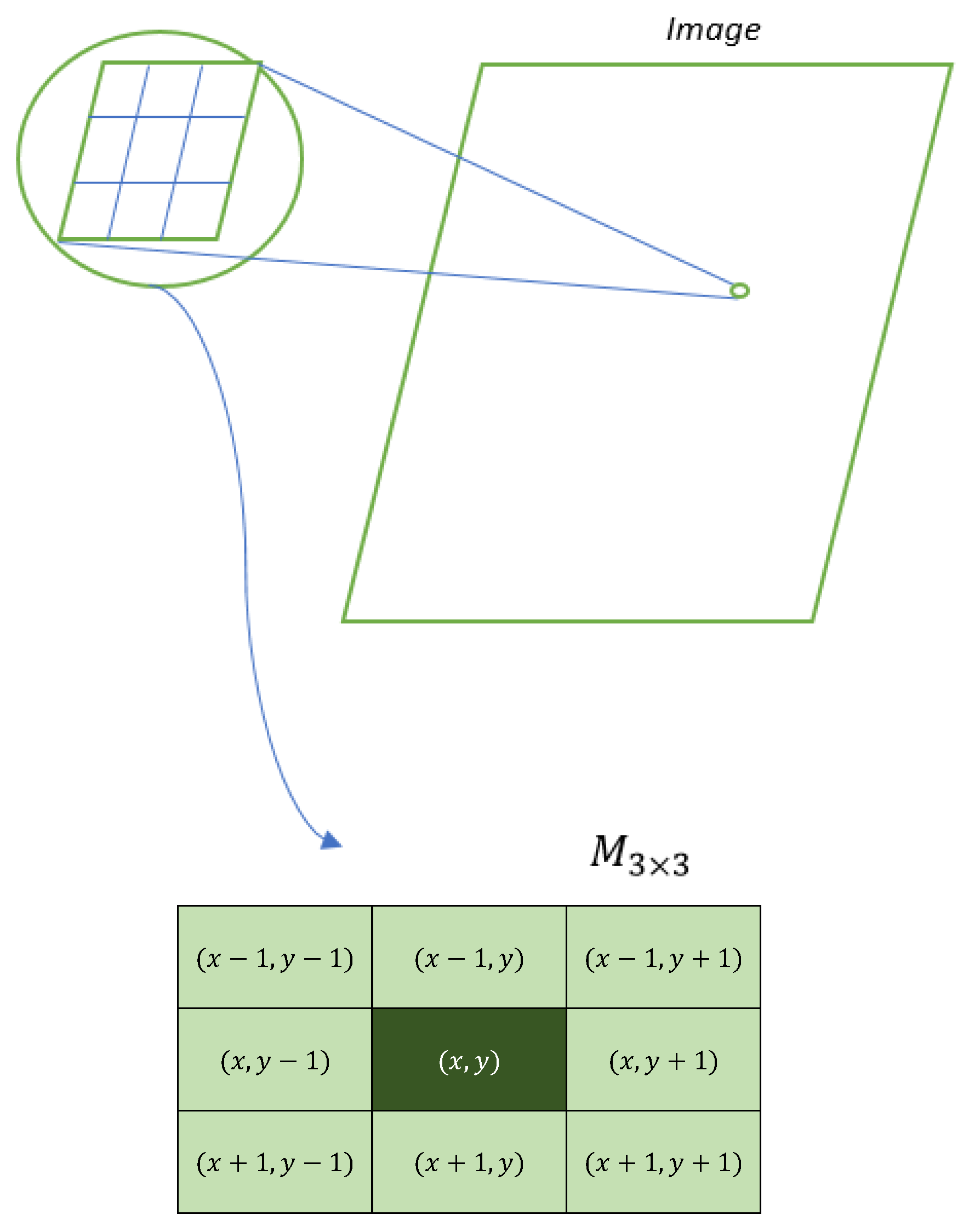
On the other hand, a matrix of dimensions $3\times 3$ or $M_{3\times 3}$ represents a part of the digital image. Each element within the matrix can be depicted in the form $M(x,y)$, which allows establishing a relative position within the matrix, as shown in Figure 3.

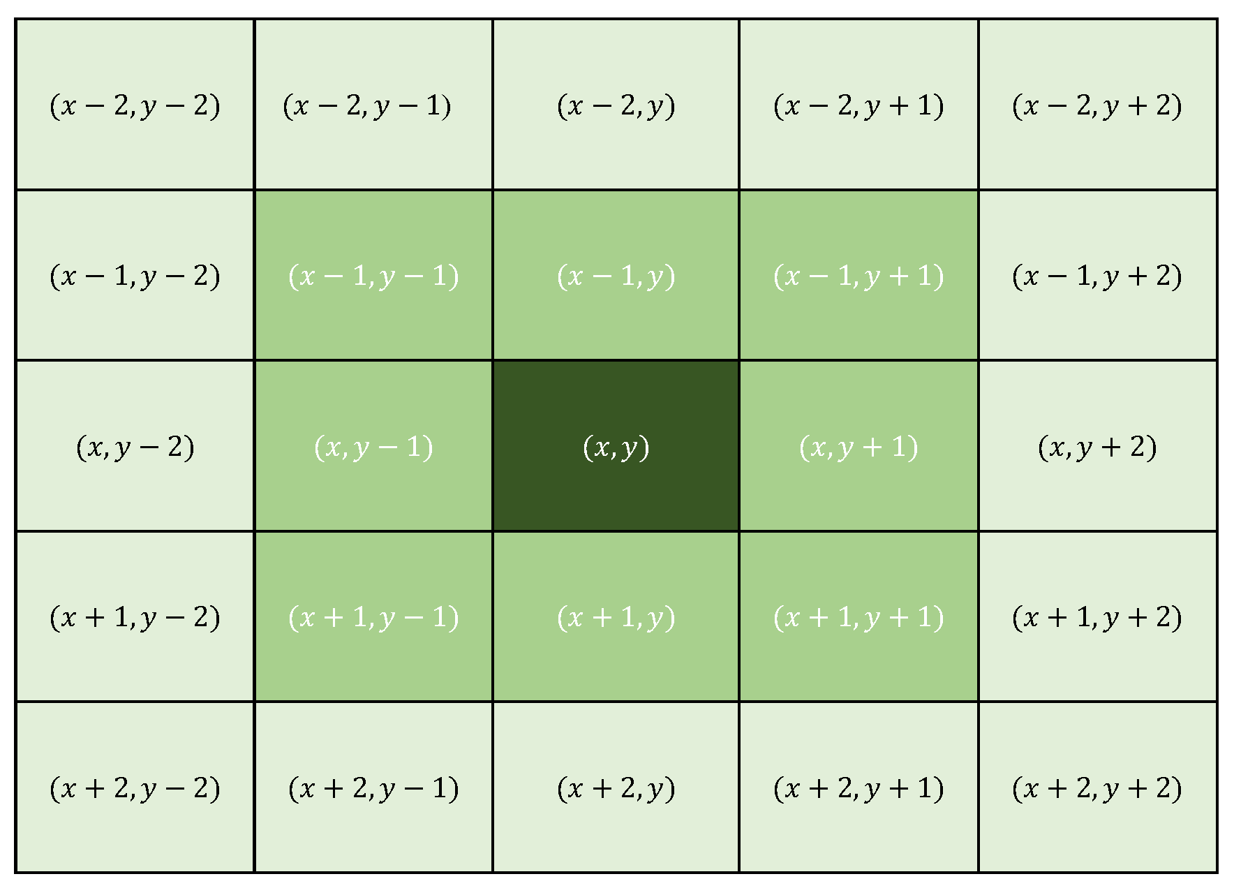
Each of the eight elements surrounding the central cell $(x,y)$ is part of the Moore neighborhood. In the DK algorithm, this neighborhood is taken with a noisy central pixel and evaluates the number of neighbors that have values 0 or 255 (possible noisy pixels). If the number of neighbors with different values of 0 or 255 is less than 5, the algorithm calculates the average of these values, and based on the neighborhood rules, it changes the value of the central pixel. Otherwise, if the number of cells with values 0 or 255 is greater than or equal to 5, then the algorithm expands the neighborhood to one of size $5\times 5$ containing the previous one (see Figure 4), this to collect more information to lead the algorithm to make the best decision.

Considering the above, a unit step function is used to turn off the function that employs the neighborhood $M_{3\times 3}$ and a new function using the neighborhood $V_{5\times 5}$ is considered to calculate the average of the values of the cells that do not have values 0 and 255. Thus, the function that models the behavior of the DK algorithm is given by Equation (4).

$$\begin{array}{c}DK(x,y)=(1-U(n-5))⌊\frac{1}{8-n}\sum _{i=-1}^1\sum _{\begin{array}{c}j=-1\\ I(x^{*},y^{*})\ne \{0,255\}\end{array}}^{1}I(x+i,y+j)-\frac{1}{8-n}I(x,y)⌋\hfill \\ \hfill -U(n-5)⌊\frac{1}{24-m}\sum _{i=-2}^2\sum _{\begin{array}{c}j=-2\\ I(x^{*},y^{*})\ne \{0,255\}\end{array}}^{2}I(x+i,y+j)-\frac{1}{24-m}I(x,y)⌋\end{array}$$

(4)

where n is the number of pixels with values 0 or 255 in the neighborhood $3\times 3$ ($M_{3\times 3}$), with $n\in 0,1,2,\dots ,8$, meanwhile m is the number of pixels with values 0 or 255 in the neighborhood $5\times 5$ ($V_{5\times 5}$) with $m\in 5,6,\dots ,24$. Finally, $I(x,y)$ is the pixel value at position $(x,y)$, and $x^{*}=x+i$, $y^{*}=y+j$.

Equation (4) can be expressed as $DK(x,y)=f_1+f_2$, in this order, function $f_1$ counts the number $(8-n)$ of cells without salt and pepper values $\{0,255\}$ and calculates the average of these values. Since the summation includes the position $(x,y)$, it is eliminated from the calculated average using $\left(\frac{-1}{8-n}I(x,y)\right)$. Finally, the result is rounded to the smallest integer employing the floor function $f\left(\alpha \right)=\lfloor \alpha \rfloor$.

$$f_1=(1-U(n-5))⌊\frac{1}{8-n}\sum _{i=-1}^1\sum _{\begin{array}{c}j=-1\\ I(x^{*},y^{*})\ne \{0,255\}\end{array}}^{1}I(x+i,y+j)-\frac{1}{8-n}I(x,y)⌋$$

(5)

On the other hand, for $f_2$ function, $U(n-5)$ is the unit step function activated when the number of pixels with salt and pepper values (0 or 255) is equal or greater than 5 in the neighborhood $3\times 3$ of the cell $(x,y)$.

$$f_2=U(n-5)⌊\frac{1}{24-m}\sum _{i=-2}^2\sum _{\begin{array}{c}j=-2\\ I(x^{*},y^{*})\ne \{0,255\}\end{array}}^{2}I(x+i,y+j)-\frac{1}{24-m}I(x,y)⌋$$

(6)

When the number of cells in the neighborhood $3\times 3$ is equal or greater than 5, the DK algorithm takes a neighborhood of size $5\times 5$ calculating the average of all the cells in that neighborhood. Given that the sum includes the position $(x,y)$, this is removed from the calculated average employing the term $\left(\frac{-1}{24-m}I(x,y)\right)$. Note that when function $U(n-5)$ turns on, $f_2$ is activated and $f_1$ deactivated. Finally, the result obtained is rounded to the smallest integer close to the calculated average.

4. Simulation Validation

In this section, a computational analysis is presented by simulation in R of the mathematical model described to evaluate the behavior of the DK algorithm compared to the conventional methods for noise elimination (median and mean filters).

In order to have simulation results with statistical validity, an experimental design based on a simple random sampling with replacement is employed, in such a way that there is a sufficient number of experiments to evaluate the performance of the algorithms. The number of experiments was determined considering what was reported in [41] for simple random sampling with replacement.

The denoising algorithms are evaluated using $3\times 3$ arrays (simulating a portion of a picture), which are randomly generated. In these experiments, the central point of this hue corresponds to the pixel with noise. Once the number of experiments (population) is defined, the noise elimination algorithms (mean, median and DK) are executed. Then, with the results obtained, the calculation of the absolute error is made to subsequently compare the results.

The experiments were carried out via a simple sampling with replacement, that is, $3\times 3$ matrix were randomly generated in the discrete interval of pixel values $[a,b]$; in this case, the size of the population is known [41]. An integer value of the interval is placed in each element of the array, except for position $M_{22}$, which can take the values 0 or 255. The size of the population is given by Equation (7), where N is divided by 8 given the symmetries of the square (according to groups theory [42]). In this way, the sample size (number of experiments) is given by Equation (8).

$$N=\frac{{(b-a+1)}^9}{8}$$

(7)

$$n=\frac{N{Z}^{2}pq}{d^2(N-1)+Z^{2}pq}$$

(8)

In Equation (8), the respective variables are:

• N: Population size.
• Z: 95% confidence level $\left(1.96\right)$.
• p: Probability of success $\left(0.5\right)$.
• q: Probability of failure $(1-p)$.
• d: Accuracy $5\%$$\left(0.05\right)$.

Simulations were made in MATLAB and the samples obtained were statistically analyzed. As an example, it is taken the pixel interval [80, 84]. In this case, the space of all possible experiments is 48,828.

It is relevant to mention that when the number of noisy pixels within the $3\times 3$ matrix is greater than half the number of non-noisy pixels (i.e., noisy pixels greater than 5), the matrix expands to a $5\times 5$ size to encompass a larger number of pixels. In this way, after determining the correct or closest value of the central pixel, the matrix returns to its original size of $3\times 3$.

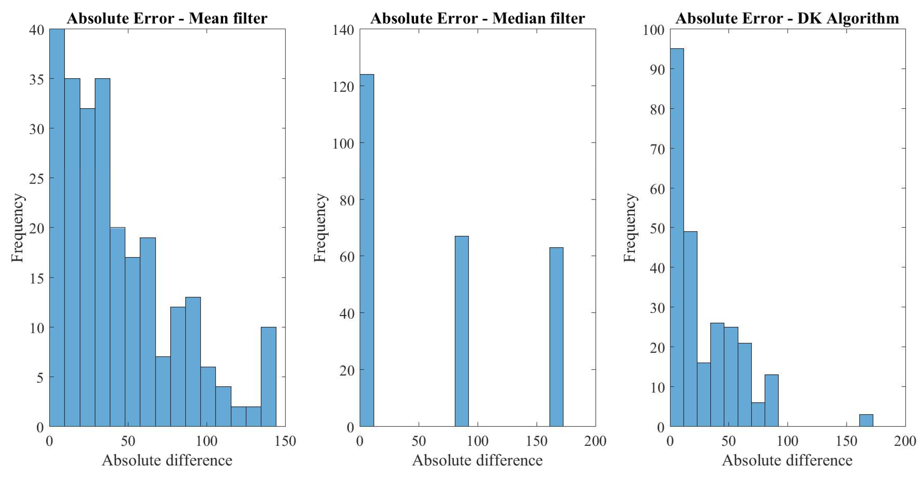
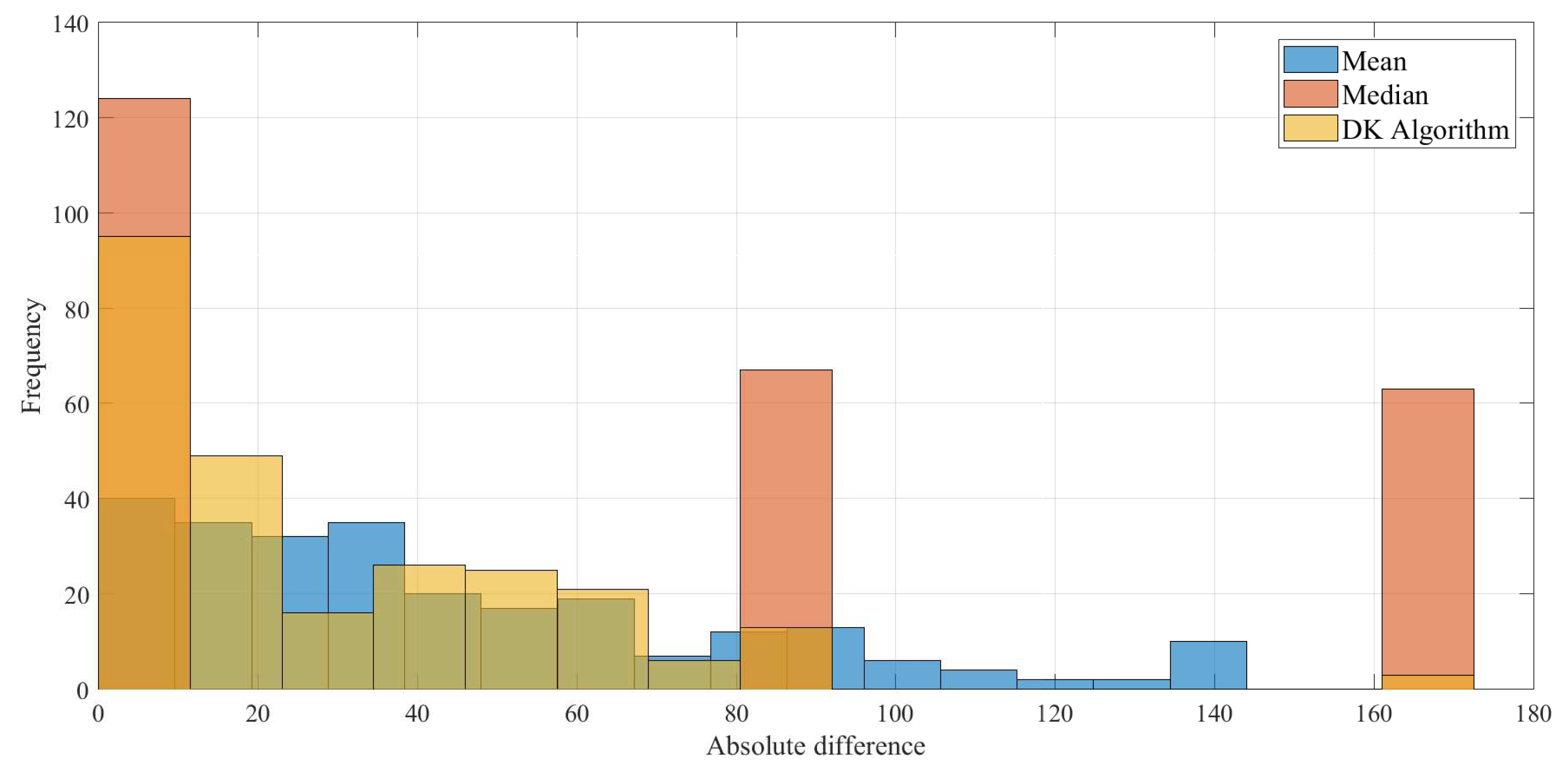
With the sampling formula, using the same values taken for the parameters, 381 masks were simulated. The absolute errors between the real value of pixel $M_{22}$ and that obtained with each of the algorithms were calculated. In this order, the histogram of the absolute error displayed in Figure 5 is obtained, where the results of each algorithm are shown separately. Figure 6 shows the histogram set of data obtained in a simulation, presenting in the same scale the results for the median, mean, and DK algorithms. In these results, the DK algorithm presents smaller values.

Regarding Figure 5 and Figure 6, it is observed that for the DK algorithm, the largest number of values of the absolute difference are close to zero. This implies that, from the total of samples obtained when executing the DK algorithm exists a greater quantity of successes at the moment of identifying the real value of the pixel. In other words, it is possible to recover the original value of the image (or a sufficiently close value) so as not to present a significant difference with the figure without noise.

In the case of the mean algorithm, although it exhibits a distribution with many values close to zero, it also presents a considerable number of pixels that are far from the real value, which implies that there are notable differences in the results after noise removal. On the other hand, the median algorithm presents results with a particular distribution (with three groups), it is observed that there is a group where the original value is recovered; however, there are two other groups far from the real value pixel, resulting in an image where impulsive noise is not satisfactorily removed.

The data were saved in three vectors and processed using the statistical software R obtaining the mean, variance, among other relevant statistical values as presented in

Table 1. Comparison of the statistics of the median and mean filters versus the DK algorithm.

Measure	Median	Mean	DK
nbr-val	381.000	381.000	381.000
nbr-null	35.000	6.000	15.000
nbr-na	0.000	0.000	0.000
min	0.000	0.000	0.000
max	175.000	147.000	175.000
range	175.000	147.000	175.000
sum	26,233.000	18,353.000	8951.000
median	80.000	41.000	15.000
mean	68.853	48.171	23.493
SE-mean	3.679	1.930	1.238
CI-mean (0.95)	7.233	3.794	2.435
var	5155.663	1418.552	584.277
std-dev	71.803	37.664	24.172
coef-var	1.043	0.782	1.029
skewness	0.447	0.794	1.994
kurtosis	−1.426	−0.237	6.947
norm-test-SW	0.767	0.920	0.807
norm-test-p	0.000	0.000	0.000

. The basic statistics are the number of values considered in the sample (nbr-val), number of null values within the sample (nbr-null), number of missing values within the sample (nbr-na), minimal value obtained (min), maximal value obtained (max), range equal to difference between max and min (range), and the sum of all non-missing values (sum). Meanwhile, the descriptive statistics are: the median (median), the mean (mean), the standard error on the mean for a given variable (SE-mean), the confidence interval for the arithmetic mean (CI-mean) at the respective p-level, the variance (var), the standard deviation (std-dev), and the variation coefficient (coef-var) equal to the standard deviation divided by the mean. Finally, the normal distribution statistics are: the skewness coefficient $g_1$ (skewness), kurtosis coefficient $g_2$ (kurtosis), statistic of a Shapiro–Wilk test of normality (norm-test-SW), and the respective associated probability (norm-test-p) [43].

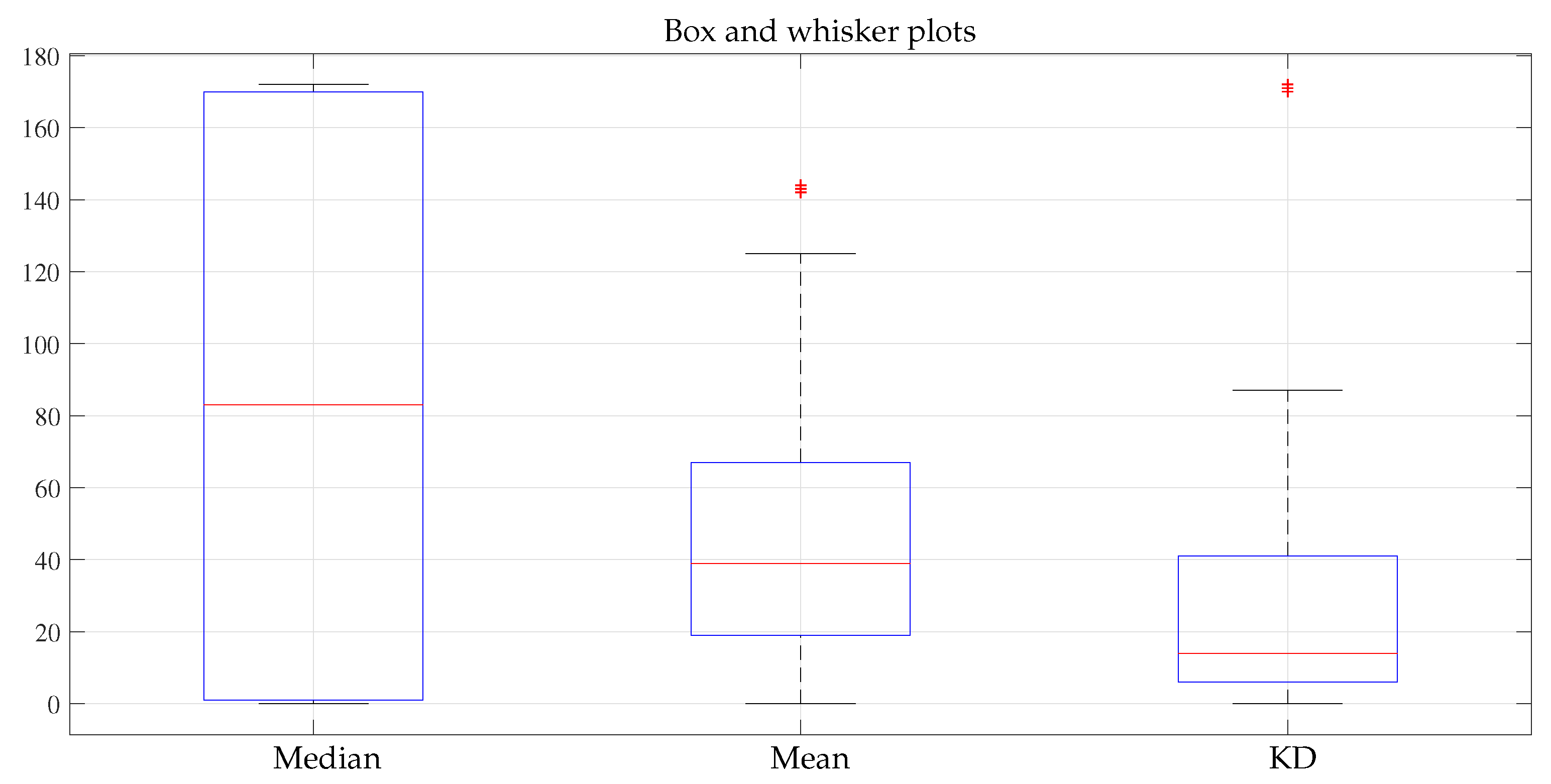
In addition, the statistical summary of the median, mean filters and DK algorithm is presented in

Table 2. Median, mean filters and DK algorithm statistical data summary.

Algorithm	Min.	1st Qu.	Median	Mean	3rd Qu.	Max.
Median	0.00	2.00	81.00	76.45	171.00	175.00
Mean	0.00	16.00	40.00	48.32	69.00	147.00
DK	0.00	7.00	15.00	23.67	35.00	171.00

. This information can be seen more compactly in the box and whisker plot shown in Figure 7.

In these results, a stronger trend is observed by the DK algorithm towards zero. Thus, on average, the data obtained with the algorithm tend to be more similar to the real values of the mask. However, as more simulations were done using fewer points with salt and pepper, the behavior of the DK algorithm and the average algorithm behaved similarly.

Additionally, calculations were made to determine the correlation of the data obtained and are presented in

Table 3. Correlation table for the simulation result.

-	Data Median	Data Mean	Data DK
Data Median	1.0000000	0.7158127	0.2821712
Data Mean	0.7158127	1.0000000	0.2301503
Data DK	0.2821712	0.2301503	1.0000000

. A positive correlation was observed between the median and mean algorithms (filters), while DK algorithm showed very little correlation between them.

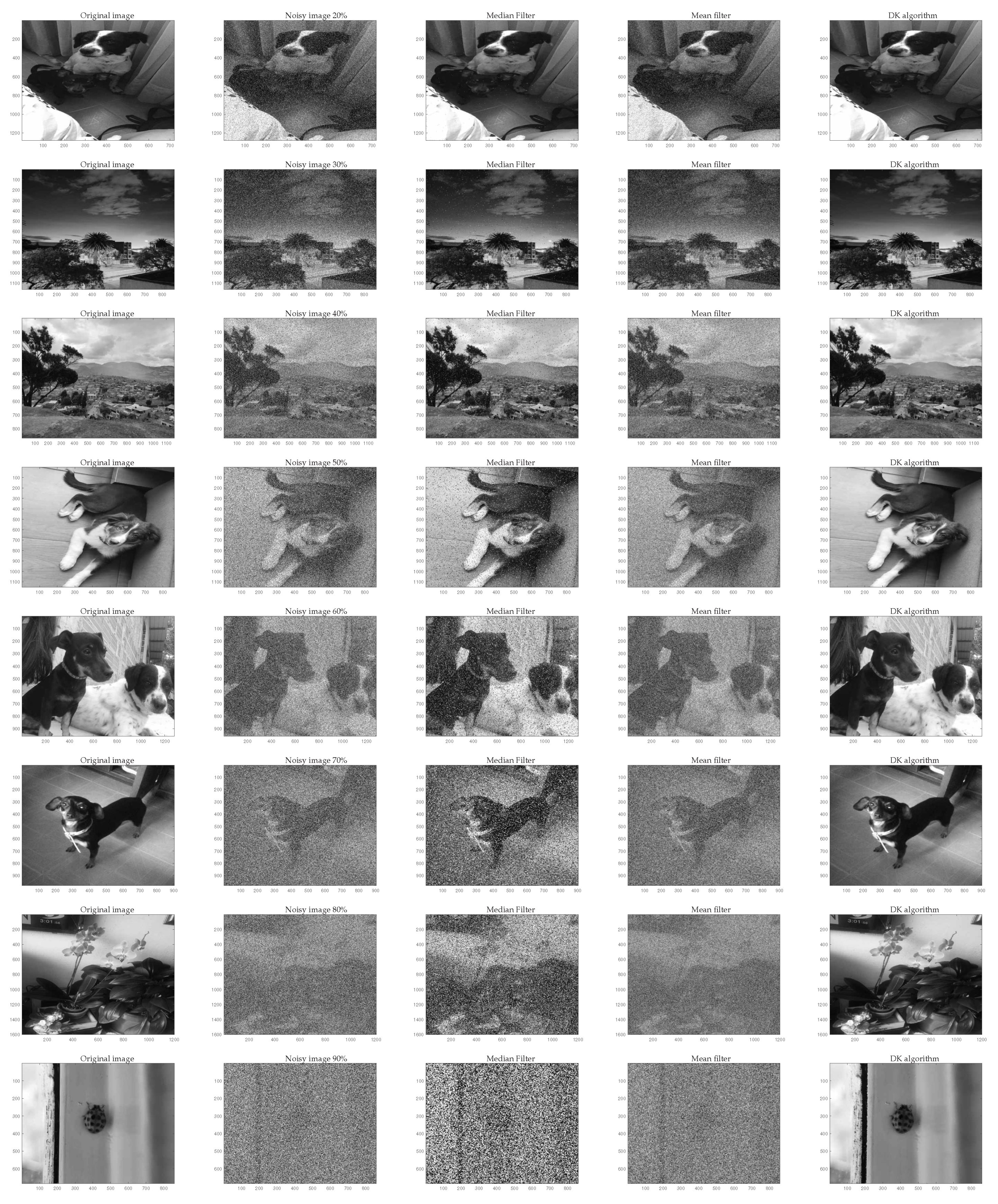
Finally, to quantitatively and qualitatively observe the algorithm performance, Figure 8 shows the elimination of noise using the mean, median and DK algorithms, where different noise values are considered for each row having $20\%$, $30\%$, $40\%$, $50\%$, $60\%$, $70\%$, $80\%$, and $90\%$ of noise level, which indicates the number of pixels contaminated in the image. Meanwhile, the first column presents the original image; later, the second column the noisy image, in the third, the image processed with the median filter; the fourth column the result with the mean filter, and finally the fifth column the filtering process with DK algorithm. As can be seen from these results, in most cases DK algorithm presents a better result than the other algorithms considered.

Considering [25,44], the Peak Signal-to-Noise Ratio (PSNR), the Signal-to-Noise Ratio (SNR), and the Structural Similarity Index Measure (SSIM) are calculated using the images in Figure 8 to evaluate the performance of DK algorithm quantitatively.

The PSNR in decibels ($dB$) is calculated using Equation (9), which employs the Mean Squared Error (MSE) given in Equation (10), where, $I_r(x,y)$ is a pixel of the original image (reference image), $I_f(x,y)$ is a pixel of the reconstructed image (filtered image), and B the number of bits employed for representing each pixel (8 bits).

$$PSNR=10{log}_{10}\left[\frac{2^B-1}{MSE}\right]dB$$

(9)

$$MSE=\frac{1}{MN}\sum _{x=1}^M\sum _{y=1}^N{[I_r(x,y)-I_f(x,y)]}^2$$

(10)

The performance index SNR in $dB$ is determined by Equation (11). This metric characterizes the quality of an image with the relationship between image power and the noise it presents [44].

$$SNR=10{log}_{10}\left[{\displaystyle \frac{{\sum }_{x=1}^M{\sum }_{y=1}^N{\left[I_r(x,y)\right]}^2}{{\sum }_{x=1}^M{\sum }_{y=1}^N{[I_r(x,y)-I_f(x,y)]}^2}}\right]dB$$

(11)

On the other hand, the SSIM is calculated via Equation (12), it is used to establish the similarity between two images, allowing us to determine how different the original image $I_r$ is from the distorted image $I_f$. Values of luminance $l(I_r,I_f)$, contrast $c(I_r,I_f)$, and structure $s(I_r,I_f)$ are used for SSIM considering $I_r$ and $I_f$ [10,25,32]. The SSIM measures between two images to compare a value between 0 and 1, where one is the absolute similarity and zero the total loss of similarity.

$$SSIM(I_r,I_f)={\left[l(I_r,I_f)\right]}^{\alpha }·{\left[c(I_r,I_f)\right]}^{\beta }·{\left[s(I_r,I_f)\right]}^{\gamma }$$

(12)

Table 4. Performance metric results, PSNR and SNR in $dB$.

Noise	Mean			Median			DK
%	PSNR	SNR	SSIM	PSNR	SNR	SSIM	PSNR	SNR	SSIM
20	17.202	9.981	0.222	23.496	16.573	0.720	42.612	32.896	0.995
30	17.430	8.192	0.187	23.474	14.237	0.757	38.251	29.013	0.988
40	15.740	6.503	0.144	18.522	9.285	0.478	36.438	27.200	0.982
50	14.799	9.901	0.098	14.925	10.027	0.197	36.088	31.190	0.957
60	11.683	6.624	0.096	12.952	7.892	0.089	34.078	29.018	0.939
70	13.684	6.524	0.065	9.935	2.776	0.028	37.862	30.703	0.938
80	10.731	4.695	0.049	7.346	1.310	0.015	32.654	26.617	0.935
90	12.148	7.636	0.049	6.504	1.992	0.007	30.095	25.584	0.931

shows the results of the metrics with different noise levels for the algorithms evaluated using the images displayed in Figure 8, as can be seen, the noise was effectively reduced in most of the levels using DK algorithm, and the similarity was always above $0.93$, which means that the filtering images with the proposed method was successful and with broad capacity to restore the image.

5. Discussion

Even though the considered cellular automata was employed in previous works [25,26,27,28], a detailed mathematical model was not addressed. Therefore, the main aspect in this paper corresponds to the mathematical description and statistical validation.

The proposed mathematical model of cellular automata can be used in a later work to carry out the respective dynamic analysis (not addressed in this work). In order to observe the algorithm features, a statistical validation for the functioning of the cellular automaton to eliminate impulsive noise is carried out.

In this paper are performed the mathematical description of the algorithm and a comparison with two very well-known algorithms, which can be considered as a comparison standard for salt and pepper noise removal. It is also relevant to mention that the algorithm is designed to eliminate salt and pepper noise, for other types of noise, it is expected to carry out the respective research to adjust the proposed algorithm.

In order to have an experimental validation, a comparison is made with two standard algorithms for impulsive noise elimination observing that DK algorithm displays a better performance; however, a broader comparison with other algorithms can be made in a further work. In this way, new strategies can also be considered to incorporate into the DK algorithm. To perform a suitable algorithm comparisons, the following aspects must be taken into account:

• Selection of the type of algorithms to be compared considering: reported performance, actuality, available code, number of citations, proposed approach of the algorithm. Some algorithms to consider consist on cellular automata-based algorithmic approaches for noise removal in digital images as Outer Totalistic Cellular Automata (OTCA) [45], and other developments like the presented in [10,46,47,48,49,50,51,52]; likewise, hybrid methods that incorporate cellular automata and fuzzy logic [32,53], as well as modifications and improvements of median filter as Unsymmetric Trimmed Median Filter (UTMF) [54], median-type noise detectors [34], and implementations using local image statistics [33]. Other approaches could also be considered, including algorithms based on dictionary learning methods [11,12], non-negative matrix factorization [13,14], and robust principal component analysis [15,16].
• Type of noise to eliminate considering different algorithms approaches. It can be considered noise additive, multiplicative, impulsive static and dynamic noise [55]. The associated probability distribution can also be considered as: uniform, Gaussian, Poisson, Rayleigh, Speckle, Gamma, White, Brownian, and other noise characteristics like periodic and structural [56].
• Performance metrics considering the operation of the algorithms, in a way that the advantages of each algorithm, can be observed as: processing time, amount of noise removed, image distortion, Mean Absolute Error (MAE), Root Mean Square Error (RMSE), Signal-to-Noise Ratio (SNR), Image Enhancement Factor (IEF), and Structural Similarity Index Measure (SSIM), that is a perceptual metric that quantifies image quality degradation caused by the processing; also the Peak Signal-to-Noise Ratio (PSNR) corresponding to the relationship between the maximum possible energy of a signal and the noise that affects it [44,45,53].
• Statistical tests to carry out the comparisons (ANOVA, Kruskal–Wallis, Bonferroni, etc.), considering assumptions of normality and equality of variance to establish the type of test (parametric and non-parametric), and in this way perform a fair comparison between algorithms [57,58].

Finally, the limitations of this work included to carry out the statistical tests the images used are synthetic considering only impulsive noise; besides, the algorithm operates on grayscale images, and no wide comparison with other types of algorithms is made.

6. Conclusions

In this work, the mathematical description of the algorithm based on a cellular automata to eliminate (reduce) noise in digital images is obtained. Various functions are incorporated into this model to complete this description.

The proposed model can be used to adapt the operation of the algorithm to carry out other processes on the digital image such as edge separation, equalization, and pattern identification.

A statistical validation of automaton cellular functioning to eliminate impulsive noise is carried out considering an experimental design based on a simple random sampling with replacement using a sufficient number of experiments to evaluate the algorithms performance.

Comparison of DK algorithm with other well-known techniques for noise removal (salt and pepper) is made. These results show that the algorithm obtains a suitable performance compared to other techniques. The denoising technique based on cellular automata can be considered as a non-linear type filtering.

According to the statistical analysis results carried out, it is observed from the correlation table that the DK algorithm presents an approximate percentage relationship of $28\%$ with respect to the median algorithm, and $23\%$ to the mean algorithm. This means that, even though the DK algorithm is based on a behavior similar to median and mean algorithms, its adaptive feature gives it the ability to expand the information with which it makes decisions and obtains effective results.

Limitations to overcome in other works are dynamic analysis of the model, also the filtering of other types of noise; operation in color images, and a wide comparison with other types of algorithms.

In a further work, the generalization of this model can be considered to be applied in color images, it can be also used to acquire or modify other color image characteristics. In addition, the application of the algorithm can also be extended to other types of noise. Besides, it could also include additional strategies in DK algorithm as neural networks, neuro-fuzzy systems, and support vector machines.

References

- Marinescu, D. Nature-Inspired Algorithms and Systems; Elsevier: Boston, MA, USA, 2017; pp. 33–63. [Google Scholar] [CrossRef]
- Gong, Y. A survey on the modeling and applications of cellular automata theory. IOP Conf. Ser. Mater. Sci. Eng. 2017, 242, 012106. [Google Scholar] [CrossRef] [Green Version]
- Das, D. A Survey on Cellular Automata and Its Applications; Springer: Berlin/Heidelberg, Germany, 2011; Volume 269. [Google Scholar] [CrossRef]
- Kolnoochenko, A.; Menshutina, N. CUDA-optimized cellular automata for diffusion limited processes. Comput. Aided Chem. Eng. 2015, 37, 551–556. [Google Scholar] [CrossRef]
- Mahata, K.; Sarkar, A.; Das, R.; Das, S. Fuzzy evaluated quantum cellular automata approach for watershed image analysis. In Quantum Inspired Computational Intelligence; Morgan Kaufmann: Boston, MA, USA, 2017; pp. 259–284. [Google Scholar] [CrossRef]
- Baxes, G. Digital Image Processing: Principles and Applications; Wiley: Hoboken, NJ, USA, 1994. [Google Scholar]
- Davies, A. The Focal Digital Imaging A-Z; Focal Press: Oxford, UK, 1998. [Google Scholar]
- Daniel, M. Optica Tradicional y Moderna; Colección “Ciencia para todos”; Fondo de Cultura Económica: Mexico City, Mexico, 2007. [Google Scholar]
- Petrou, M.; Petrou, C. Image Processing: The Fundamentals; Wiley: Hoboken, NJ, USA, 2010. [Google Scholar]
- Tourtounis, D.; Mitianoudis, N.; Sirakoulis, G.C. Salt-n-pepper Noise Filtering using Cellular Automata. J. Cell. Autom. 2018, 13, 81–101. [Google Scholar]
- Cai, S.; Kang, Z.; Yang, M.; Xiong, X.; Peng, C.; Xiao, M. Image Denoising via Improved Dictionary Learning with Global Structure and Local Similarity Preservations. Symmetry 2018, 10, 167. [Google Scholar] [CrossRef] [Green Version]
- Peng, C.; Cheng, Q. Discriminative Ridge Machine: A Classifier for High-Dimensional Data or Imbalanced Data. IEEE Trans. Neural Net. Learn. Syst. 2021, 32, 2595–2609. [Google Scholar] [CrossRef] [PubMed]
- Farouk, R.M.; Khalil, H.A. Image Denoising based on Sparse Representation and Non-Negative Matrix Factorization. Life Sci. J. 2012, 9, 337–341. [Google Scholar]
- Peng, C.; Zhang, Z.; Kang, Z.; Chen, C.; Cheng, Q. Nonnegative matrix factorization with local similarity learning. Inf. Sci. 2021, 562, 325–346. [Google Scholar] [CrossRef]
- Liu, Y.; Zhang, Q.; Chen, Y.; Cheng, Q.; Peng, C. Hyperspectral Image Denoising With Log-Based Robust PCA. In Proceedings of the 2021 IEEE International Conference on Image Processing (ICIP), Anchorage, AK, USA, 19–22 September 2021; pp. 1634–1638. [Google Scholar] [CrossRef]
- Peng, C.; Chen, Y.; Kang, Z.; Chen, C.; Cheng, Q. Robust principal component analysis: A factorization-based approach with linear complexity. Inf. Sci. 2020, 513, 581–599. [Google Scholar] [CrossRef]
- Vezhnevets, V.; Konushin, V. “GrowCut”—Interactive Multi-Label ND Image Segmentation By Cellular Automata. Graphicon 2004, 1, 150–156. [Google Scholar]
- Marginean, R.; Andreica, A.; Diosan, L.; Bálint, Z. Feasibility of Automatic Seed Generation Applied to Cardiac MRI Image Analysis. Mathematics 2020, 8, 1511. [Google Scholar] [CrossRef]
- Marginean, R.; Andreica, A.; Diosan, L.; Bálint, Z. Butterfly Effect in Chaotic Image Segmentation. Entropy 2020, 22, 1028. [Google Scholar] [CrossRef] [PubMed]
- Velasquez, W.; Alvarez-Alvarado, M.S. Outdoors Evacuation Routes Algorithm Using Cellular Automata and Graph Theory for Uphills and Downhills. Sustainability 2021, 13, 4731. [Google Scholar] [CrossRef]
- Mărginean, R.; Andreica, A.; Dioşan, L.; Bálint, Z. A Transfer Learning Approach on the Optimization of Edge Detectors for Medical Images Using Particle Swarm Optimization. Entropy 2021, 23, 414. [Google Scholar] [CrossRef]
- Fuente, D.; Garibo i Orts, O.; Conejero, J.A.; Urchueguía, J.F. Rational Design of a Genetic Finite State Machine: Combining Biology, Engineering, and Mathematics for Bio-Computer Research. Mathematics 2020, 8, 1362. [Google Scholar] [CrossRef]
- Treml, L.M.; Bartocci, E.; Gizzi, A. Modeling and Analysis of Cardiac Hybrid Cellular Automata via GPU-Accelerated Monte Carlo Simulation. Mathematics 2021, 9, 164. [Google Scholar] [CrossRef]
- Rößler, C.; Breitenecker, F.; Riegler, M. Simulating the Gluing of Wood Particles by Lattice Gas Cellular Automata and Random Walk. Mathematics 2020, 8, 988. [Google Scholar] [CrossRef]
- Angulo, K.; Gil, D.; Espitia, H. A novel algorithm based on cellular automata to eliminate noise in digital images. J. Eng. Appl. Sci. 2019, 14, 3289–3300. [Google Scholar]
- Gil-Sierra, D.G.; Angulo-Sogamoso, K.V.; Espitia-Cuchango, H.E. Integration of an adaptive cellular automaton and a cellular neural network for the impulsive noise suppression and edge detection in digital images. In Proceedings of the 2019 IEEE Colombian Conference on Applications in Computational Intelligence (ColCACI), Barranquilla, Colombia, 5–7 June 2019; pp. 1–6. [Google Scholar] [CrossRef]
- Angulo, K.; Gil, D.; Espitia, H. Integration of an Adaptive Cellular Automaton and a Cellular Neural Network for the Impulsive Noise Suppression and Edge Detection in Digital Images. In Applications of Computational Intelligence. ColCACI 2019. Communications in Computer and Information Science; Orjuela-Cañón, A., Figueroa-García, J., Arias-Londoño, J., Eds.; Springer: Cham, Switzerland, 2019; Volume 1096, pp. 168–181. [Google Scholar] [CrossRef]
- Angulo, K.; Gil, D.; Espitia, H. Method for Edges Detection in Digital Images Through the Use of Cellular Automata. In Advances and Applications in Computer Science, Electronics and Industrial Engineering. CSEI 2019. Advances in Intelligent Systems and Computing; Nummenmaa, J., Pérez-González, F., Domenech-Lega, B., Vaunat-J, O., Fernández-Peña, F., Eds.; Springer: Cham, Switzerland, 2020; Volume 1078, pp. 3–21. [Google Scholar] [CrossRef]
- Pyt’ev, Y. Mathematical Methods of Subjective Modeling in Scientific Research: I. The Mathematical and Empirical Basis. Mosc. Univ. Phys. Bull. 2018, 73, 1–16. [Google Scholar] [CrossRef]
- Ouvrier-Buffet, C. Exploring Mathematical Definition Construction Processes. Educ. Stud. Math. 2006, 63, 259–282. [Google Scholar] [CrossRef]
- Menskii, M.B. The difficulties in the mathematical definition of path integrals are overcome in the theory of continuous quantum measurements. Theor. Math. Phys. 1992, 93, 1262–1267. [Google Scholar] [CrossRef]
- Sahin, U.; Uguz, S.; Sahin, F. Salt and pepper noise filtering with fuzzy-cellular automata. Comput. Electr. Eng. 2014, 40, 59–69. [Google Scholar] [CrossRef]
- Garnett, R.; Huegerich, T.; Chui, C.; He, W. A universal noise removal algorithm with an impulse detector. IEEE Trans. Image Process. 2005, 14, 1747–1754. [Google Scholar] [CrossRef] [PubMed] [Green Version]
- Chan, R.; Ho, C.W.; Nikolova, M. Salt-and-pepper noise removal by median-type noise detectors and detail-preserving regularization. IEEE Trans. Image Process. 2005, 14, 1479–1485. [Google Scholar] [CrossRef]
- Salcido, A. Cellular Automata: Simplicity Behind Complexity; IntechOpen: Rijeka, Croatia, 2011. [Google Scholar]
- Schiff, J. Cellular Automata: A Discrete View of the World; Wiley Series in Discrete Mathematics & Optimization; Wiley: Hoboken, NJ, USA, 2011. [Google Scholar]
- Pan, P.Z.; Feng, X.T.; Zhou, H. Solid Cellular Automaton Method for the Solution of Physical Field. In Proceedings of the 2009 WRI World Congress on Computer Science and Information Engineering, Los Angeles, CA, USA, 31 March–2 April 2009; Volume 1, pp. 765–768. [Google Scholar] [CrossRef]
- Shukla, A.P. Training Cellular Automata for Image Edge Detection. Rom. J. Inf. Sci. Technol. 2016, 19, 338–359. [Google Scholar]
- Rosin, P.; Adamatzky, A.; Sun, X. Cellular Automata in Image Processing and Geometry; Springer: Cham, Switzerland, 2014. [Google Scholar] [CrossRef]
- Wongthanavasu, S.; Sadananda, R. A CA-based edge operator and its performance evaluation. J. Vis. Commun. Image Represent. 2003, 14, 83–96. [Google Scholar] [CrossRef]
- Rodríguez del Águila, M.; González-Ramírez, A. Sample size calculation. Allergol. Immunopathol. 2014, 42, 485–492. [Google Scholar] [CrossRef] [PubMed]
- Caicedo, J. Teoría de Grupos; Universidad Nacional de Colombia, Facultad de Ciencias: Bogotá, Colombia, 2004. [Google Scholar]
- Github. Descriptive Statistics. 2022. Available online: https://sdesabbata.github.io/granolarr_v1/Lectures/bookdown/descriptive-statistics.html (accessed on 19 July 2021).
- Gonzalez, R.; Woods, R. Digital Image Processing; Pearson/Prentice Hall: Hoboken, NJ, USA, 2008. [Google Scholar]
- Jeelani, Z.; Qadir, F. Cellular automata-based approach for salt-and-pepper noise filtration. J. King Saud Univ.-Comput. Inf. Sci. 2022, 34, 365–374. [Google Scholar] [CrossRef]
- Qadir, F.; Shoosha, I.Q. Cellular automata-based efficient method for the removal of high-density impulsive noise from digital images. Int. J. Inf. Technol. 2018, 10, 529–536. [Google Scholar] [CrossRef]
- Qadir, F.; Peer, M.A.; Khan, K.A. Cellular automata based identification and removal of impulsive noise from corrupted images. J. Glob. Res. Comput. Sci. 2012, 3, 17–20. [Google Scholar]
- Jana, B.; Pal, P.; Bhaumik, J. New Image Noise Reduction Schemes Based on Cellular Automata. Int. J. Soft Comput. Eng. 2012, 2, 98–104. [Google Scholar]
- Wongthanavasu, S. Cellular Automata for Medical Image Processing. In Cellular Automata; Salcido, A., Ed.; IntechOpen: Rijeka, Croatia, 2011. [Google Scholar] [CrossRef] [Green Version]
- Rosin, P.L. Image processing using 3-state cellular automata. Comput. Vis. Image Underst. 2010, 114, 790–802. [Google Scholar] [CrossRef]
- Selvapeter, P.J.; Hordijk, W. Cellular automata for image noise filtering. In Proceedings of the 2009 World Congress on Nature Biologically Inspired Computing (NaBIC), Coimbatore, India, 9–11 December 2009; pp. 193–197. [Google Scholar] [CrossRef]
- Rosin, P.L. Training Cellular Automata for Image Processing. In Image Analysis. SCIA 2005. Lecture Notes in Computer Science; Kalviainen, H., Parkkinen, J., Kaarna, A., Eds.; Springer: Berlin/Heidelberg, Germany, 2005; pp. 195–204. [Google Scholar] [CrossRef] [Green Version]
- Piroozmandan, M.M.; Farokhi, F.; Kangarloo, K.; Jahanshahi, M. Removing the impulse noise from images based on fuzzy cellular automata by using a two-phase innovative method. Optik 2022, 255, 168713. [Google Scholar] [CrossRef]
- Esakkirajan, S.; Veerakumar, T.; Subramanyam, A.N.; PremChand, C.H. Removal of High Density Salt and Pepper Noise Through Modified Decision Based Unsymmetric Trimmed Median Filter. IEEE Signal Process. Lett. 2011, 18, 287–290. [Google Scholar] [CrossRef]
- Owotogbe, J.S.; Ibiyemi, T.S.; Adu, B.A. A Comprehensive Review On Various Types of Noise in Image Processing. Int. J. Sci. Eng. Res. 2019, 10, 388–393. [Google Scholar]
- Patro, P.; Panda, C. A review on: Noise model in digital image processing. Int. J. Eng. Sci. Res. Technol. 2016, 5, 891–897. [Google Scholar]
- De Canditiis, D. Statistical Inference Techniques. In Encyclopedia of Bioinformatics and Computational Biology; Ranganathan, S., Gribskov, M., Nakai, K., Schönbach, C., Eds.; Academic Press: Oxford, UK, 2019; pp. 698–705. [Google Scholar] [CrossRef]
- Lewis, C. Multiple Comparisons. In International Encyclopedia of Education, 3rd ed.; Peterson, P., Baker, E., McGaw, B., Eds.; Elsevier: Oxford, UK, 2010; pp. 312–318. [Google Scholar] [CrossRef]
Publisher’s Note: MDPI stays neutral with regard to jurisdictional claims in published maps and institutional affiliations. |
© 2022 by the authors. Licensee MDPI, Basel, Switzerland. This article is an open access article distributed under the terms and conditions of the Creative Commons Attribution (CC BY) license (https://creativecommons.org/licenses/by/4.0/).