
Modeling the Effect of the Spatial Pattern of Airborne Lidar Returns on the Prediction and the Uncertainty of Timber Merchantable Volume


Abstract
1. Introduction
2. Materials and Methods
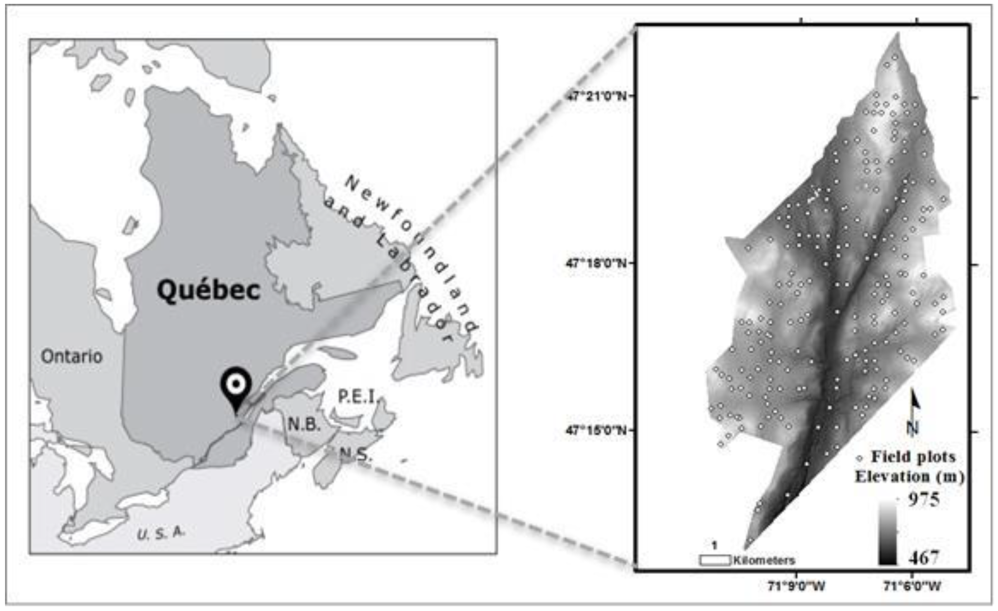
2.1. Study Area
2.2. Field Plot Data
2.3. Lidar Data
2.4. Data Analysis
2.4.1. Generalized Least Squares in Nonlinear Regression
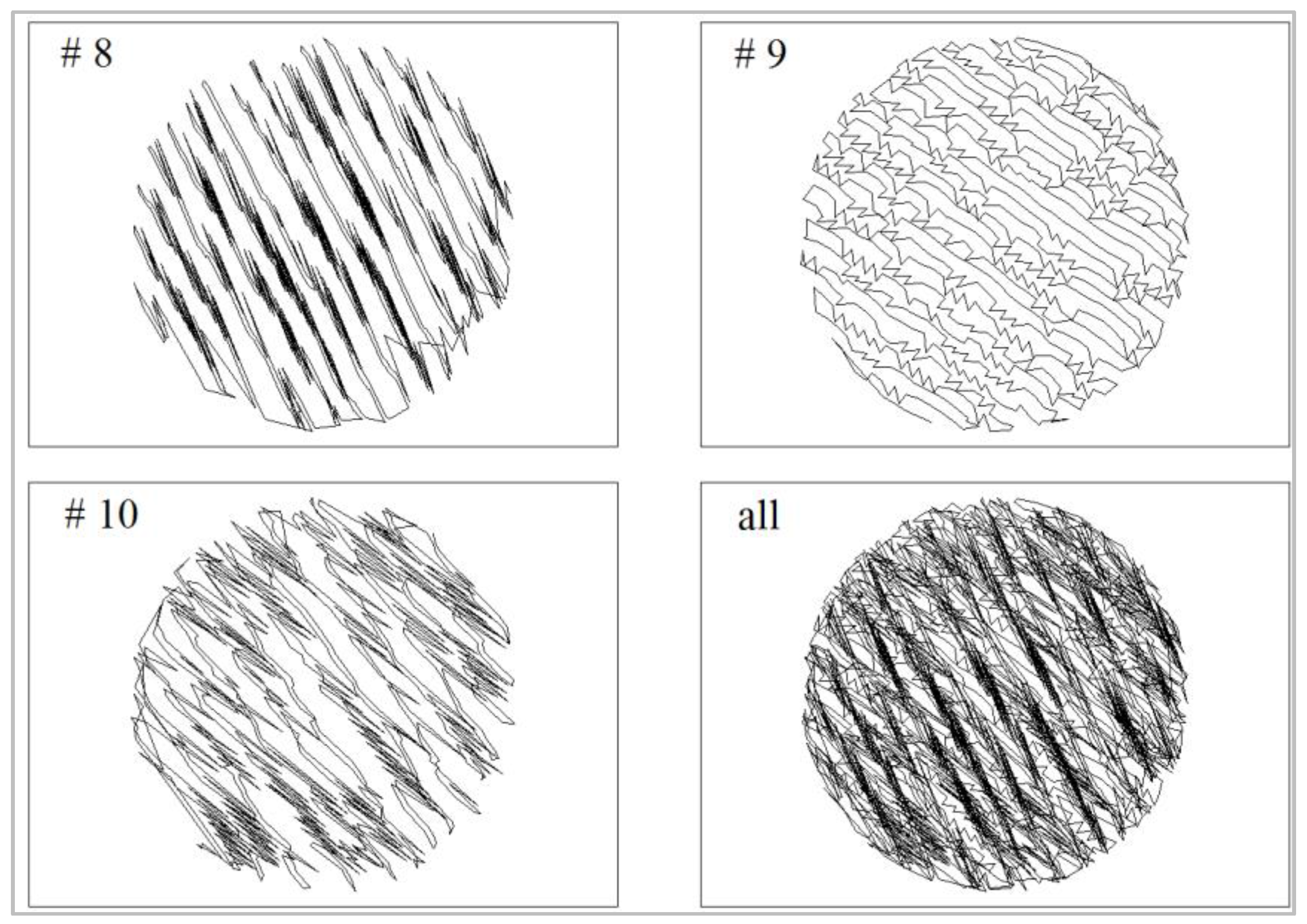
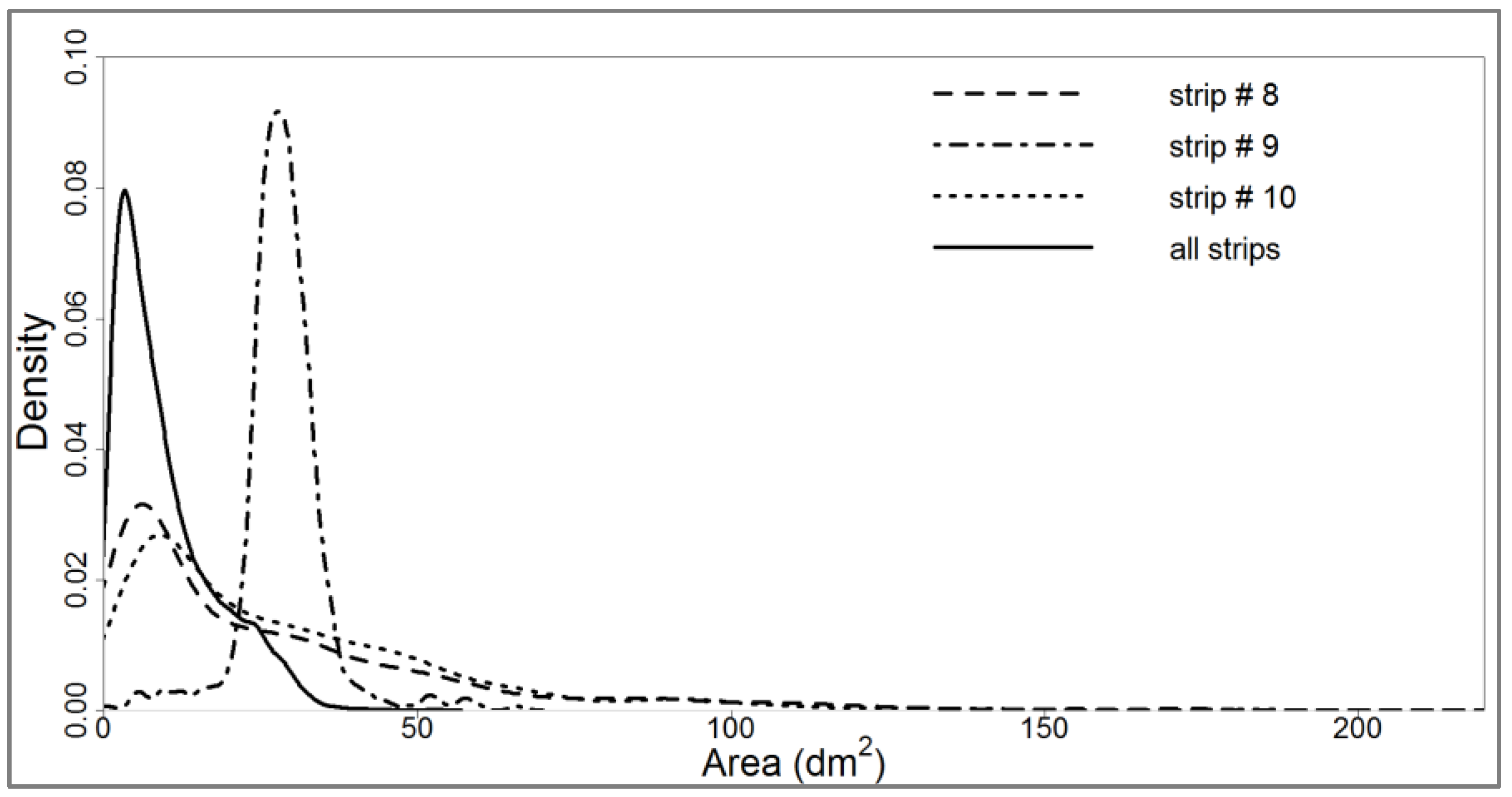
2.4.2. Analysis of the Spatial Distribution of Returns
2.4.3. Lidar Variable Generation
2.4.4. Establishing the Merchantable Volume Model
2.4.5. Residual Variance
2.4.6. Model Validation
3. Results
4. Discussion
5. Conclusions
Acknowledgments
Author Contributions
Conflicts of Interest
References
- Gatziolis, D.; Andersen, H.-E. A Guide to LIDAR Data Acquisition and Processing for the Forests of the Pacific Northwest; U.S. Department of Agriculture, Forest Service, Pacific Northwest Research Station: Washington, DC, USA, 2008.
- Korpela, I.; Ørka, H.O.; Maltamo, M.; Tokola, T.; Hyyppä, J. Tree species classification using airborne LiDAR—Effects of stand and tree parameters, downsizing of training set, intensity normalization, and sensor type. Silva Fenn. 2010, 44, 319–339. [Google Scholar] [CrossRef]
- Balsa-Barreiro, J.; Pere, J.P.; Lerma, J.L. Airborne Light Detection and Ranging (LiDAR) point density analysis. Sci. Res. Essays 2012, 7, 3010–3019. [Google Scholar] [CrossRef]
- Ehlert, D.; Heisig, M. Sources of angle-dependent errors in terrestrial laser scanner-based crop stand measurement. Comput. Electron. Agric. 2013, 93, 10–16. [Google Scholar] [CrossRef]
- Balsa-Barreiro, J.; Lerma, J.L. Empirical study of variation in lidar point density over different land covers. Int. J. Remote Sens. 2014, 35, 3372–3383. [Google Scholar] [CrossRef]
- Isenburg, M. LAStools—Efficient Lidar Processing Software, version 150526, unlicensed; Available online: http://www.rapidlasso.com/LAStools (accessed on 1 May 2017).
- McGaughey, R.J. FUSION/LDV: Software for LIDAR Data Analysis and Visualization; version 3.42.; USDA Forest Service: Washington, DC, USA, 2014; Volume 175.
- Bouvier, M.; Durrieu, S.; Fournier, R.A.; Renaud, J.-P. Generalizing predictive models of forest inventory attributes using an area-based approach with airborne lidar data. Remote Sens. Environ. 2015, 156, 322–334. [Google Scholar] [CrossRef]
- Maltamo, M.; Eerikäinen, K.; Packalén, P.; Hyyppä, J. Estimation of stem volume using laser scanning-based canopy height metrics. Forestry 2006, 79, 217–229. [Google Scholar] [CrossRef]
- Næsset, E. Accuracy of forest inventory using airborne laser scanning: Evaluating the first nordic full-scale operational project. Scand. J. For. Res. 2004, 19, 554–557. [Google Scholar] [CrossRef]
- Treitz, P.; Lim, K.; Woods, M.; Pitt, D.; Nesbitt, D.; Etheridge, D. LiDAR sampling density for forest resource inventories in Ontario, Canada. Remote Sens. 2012, 4, 830–848. [Google Scholar] [CrossRef]
- Beal, S.L.; Sheiner, L.B. Heteroscedastic nonlinear regression. Technometrics 1988, 30, 327–338. [Google Scholar] [CrossRef]
- Wolter, K.M. Introduction to Variance Estimation; Springer Science & Business Media: Berlin, Germany, 2007; pp. 384–389. [Google Scholar]
- Holopainen, M.; Mäkinen, A.; Rasinmäki, J.; Hyytiäinen, K.; Bayazidi, S.; Vastaranta, M.; Pietilä, I. Uncertainty in forest net present value estimations. Forests 2010, 1, 177–193. [Google Scholar] [CrossRef]
- Pinheiro, J.; Bates, D. Mixed-Effects Models in S and S-PLUS; Statistics and Computing Series; Springer: New York, NY, USA, 2000. [Google Scholar]
- Worrall, J.J.; Egeland, L.; Eager, T.; Mask, R.A.; Johnson, E.W.; Kemp, P.A.; Shepperd, W.D. Rapid mortality of Populus tremuloides in southwestern Colorado, USA. For. Ecol. Manag. 2008, 255, 686–696. [Google Scholar] [CrossRef]
- Ruppert, D. Transformation and weighting. In The Work of Raymond J. Carroll; Springer: New York, NY, USA, 2014; pp. 155–194. [Google Scholar]
- Næsset, E. Effects of different flying altitudes on biophysical stand properties estimated from canopy height and density measured with a small-footprint airborne scanning laser. Remote Sens. Environ. 2004, 91, 243–255. [Google Scholar] [CrossRef]
- Morsdorf, F.; Frey, O.; Meier, E.; Itten, K.I.; Allgoewer, B. Assessment of the influence of flying altitude and scan angle on biophysical vegetation products derived from airborne laser scanning. Int. J. Remote Sens. 2008, 29, 1387–1406. [Google Scholar] [CrossRef]
- Canada Environment and Natural Resources. 1971–2000 Climate Normals & Averages. Available online: http://climate.weather.gc.ca/climate_normals/index_e.html (accessed on 1 May 2017).
- Bélanger, L. La forêt mosaïque comme stratégie de conservation de la biodiversité de la sapinière boréale de l’Est: l’Expérience de la forêt Montmorency–Mosaic cutting as a biodiversity conservation strategy in eastern boreal balsam fir forests: The case study of the Montmorency forest. Nat. Can. 2001, 125, 18–25. [Google Scholar]
- Fortin, M.; DeBlois, J.; Bernier, S.; Blais, G. Mise au point d’un tarif de cubage général pour les forêts québécoises: Une approche pour mieux évaluer l’incertitude associée aux prévisions—Establishing a general cubic volume table for Québec forests: An approach to better assess prediction uncertainties. For. Chron. 2007, 83, 754–765. [Google Scholar]
- Kane, R.; McGaughey, R.J.; Bakker, J.D.; Gersonde, R.F.; Lutz, J.A.; Franklin, J.F. Comparisons between field- and Lidar-based measures of stand structural complexity. Can. J. For. Res. 2010, 40, 761–773. [Google Scholar] [CrossRef]
- Van Breugel, P. r.vif: A GRASS GIS Addon for Stepwise Variance Inflation Factor Variable Selection. Available online: https://www.researchgate.net/publication/301560324_rvif_A_GRASS_GIS_addon_for_stepwise_variance_inflation_factor_variable_selection (accessed on 1 May 2017).
- R Core Team. R: A Language and Environment for Statistical Computing. Available online: https://rdrr.io/cran/nlme/ (accessed on 1 May 2017).
- Pinheiro, J.; Bates, D.; DebRoy, S.; Sarkar, D.; R Core Team. nlme: Linear and Nonlinear Mixed Effects Models, version 3.1-131. Available online: http://www.gbif.org/resource/81287 (accessed on 1 May 2017).
- Robinson, A.P.; Hamann, J.D. Forest Analytics with R: An Introduction; Springer: New York, NY, USA, 2011; p. 339. [Google Scholar]
- Luther, J.E.; Skinner, R.; Fournier, R.A.; van Lier, O.R.; Bowers, W.W.; Coté, J.-F.; Hopkinson, C.; Moulton, T. Predicting wood quantity and quality attributes of balsam fir and black spruce using airborne laser scanner data. Forestry 2013, 87, 313–326. [Google Scholar] [CrossRef]
- Woods, M.; Pitt, D.; Penner, M.; Lim, K.; Nesbitt, D.; Etheridge, D.; Treitz, P. Operational implementation of a LiDAR inventory in Boreal Ontario. For. Chron. 2011, 87, 512–528. [Google Scholar] [CrossRef]
- St-Onge, B.; Vepakomma, U.; Sénécal, J.-F.; Kneeshaw, D.; Doyon, F. Canopy gap detection and analysis with airborne laser scanning. In Forestry Applications of Airborne Laser Scanning; Springer: New York, NY, USA, 2014; pp. 419–437. [Google Scholar]
- Laiho, O.; Lähde, E.; Pukkala, T. Uneven-vs even-aged management in Finnish boreal forests. Forestry 2011, 84, 547–556. [Google Scholar] [CrossRef]
- Ohara, K.L. Dynamics and stocking-level relationships of multi-aged ponderosa pine stands. For. Sci. 1996, 33, a0001. [Google Scholar]
- Puetz, A.M.; Olsen, R.C.; Anderson, B. Effects of lidar point density on bare earth extraction and DEM creation. In SPIE Defense, Security, and Sensing; International Society for Optics and Photonics: Bellingham, WA, USA, 2009. [Google Scholar]
- Vaze, J.; Teng, J.; Spencer, G. Impact of DEM accuracy and resolution on topographic indices. Environ. Model. Softw. 2010, 25, 1086–1098. [Google Scholar] [CrossRef]
- Spies, T.A.; Franklin, J.F. The structure of natural young, mature, and old-growth Douglas-fir forests in Oregon and Washington. In Wildlife and Vegetation of Unmanaged Douglas-Fir Forests; U.S. Department of Agriculture, Forest Service, Pacific Northwest Research Station: Washington, DC, USA, 1991; pp. 91–109. [Google Scholar]
- Thomas, V.; Treitz, P.; McCaughey, J.; Morrison, I. Mapping stand-level forest biophysical variables for a mixedwood boreal forest using lidar: An examination of scanning density. Can. J. For. Res. 2006, 36, 34–47. [Google Scholar] [CrossRef]
- Næsset, E. Assessing sensor effects and effects of leaf-off and leaf-on canopy conditions on biophysical stand properties derived from small-footprint airborne laser data. Remote Sens. Environ. 2005, 98, 356–370. [Google Scholar] [CrossRef]


| Field Attributes | Mean | Std. | Range |
|---|---|---|---|
| Diameter at breast height (cm) | 21.9 | 5.2 | 13.3–38.0 |
| Dominant height (m) | 15.1 | 4.2 | 9.2–26.6 |
| Density (trees ha−1) | 1433.0 | 536.0 | 117.0–3078.0 |
| Basal area (m2 ha−1) | 25.8 | 10.9 | 3.7–49.5 |
| Merchantable volume (m3 ha−1) | 144.1 | 90.2 | 21.0–411.9 |
| Lidar Attributes | Mean | Std. | Range |
|---|---|---|---|
| Mean_h (m) | 5.9 | 2.2 | 1.7–11.5 |
| Above-ground density (m−2) | 6.4 | 1.8 | 3.2–12.5 |
| Above-ground spacing (dm) | 4 | 1 | 3–6 |
| Scanning angle (°) | 9.1 | 4.7 | 0.0–24.0 |
| Skew_area | 1.4 | 0.5 | 0.4–3.9 |
| Prop_2m (%) | 15.3 | 13.9 | 0.2–63.5 |
| Ri | 2.7 | 0.7 | 1.6–5.2 |
| Before (no Variance Function) | After (with Variance Function) | ||||||||
|---|---|---|---|---|---|---|---|---|---|
| Value | Std. Err. | p-Value | 95% CI | Value | Std. Err. | p-Value | 95% CI | ||
| Parameters of the fixed part of the model | Variables | ||||||||
| Intercept | 2.04 | 0.17 | <0.001 | [1.77–2.42] | 1.97 | 0.16 | <0.001 | [1.76–2.34] | |
| Mean_h | 1.33 | 0.10 | <0.001 | [1.14–1.52] | 1.33 | 0.11 | <0.001 | [1.12–1.55] | |
| Prop_2m | −0.08 | 0.03 | 0.020 | [−0.13–−0.02] | −0.07 | 0.03 | 0.020 | [−0.07–−0.02] | |
| Ri | 0.64 | 0.12 | <0.001 | [0.40–0.88] | 0.71 | 0.13 | <0.001 | [0.64–0.87] | |
| Parameters of the variance function | Variables | ||||||||
| Mean_h | --- | --- | --- | --- | 0.85 | <0.001 | [0.50–1.20] | ||
| Skew_area | --- | --- | --- | --- | 0.31 | <0.001 | [0.05–0.57] | ||
| MV Model | AICc | p-Value | Pseudo R2 | RSD |
|---|---|---|---|---|
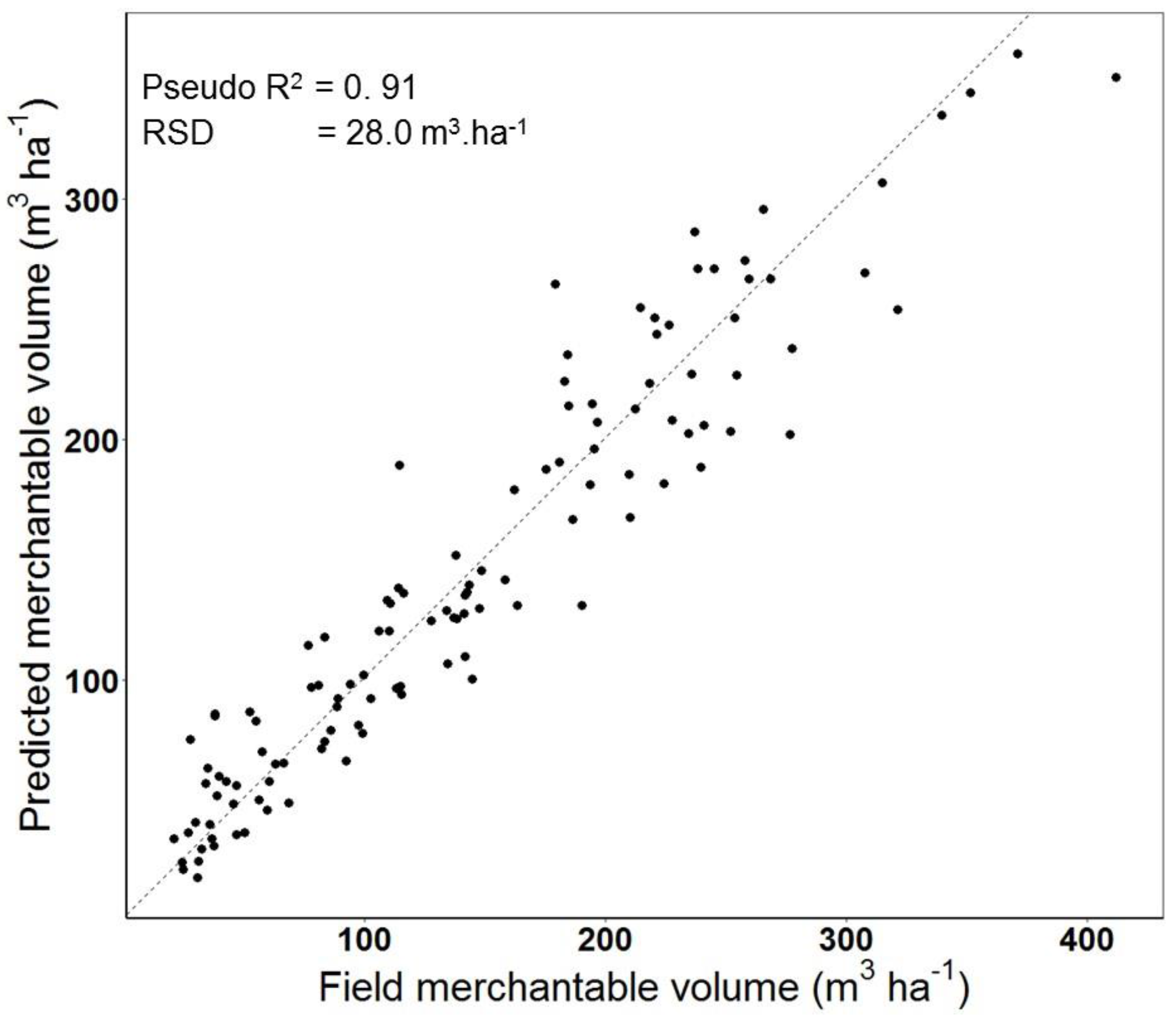
| Basic model | 1137.23 | <0.001 | 0.91 | 28.0 |
| Basic model + Density | 1139.32 | 0.74 * | 0.91 | 28.0 |
| Basic model + Mean_angle | 1137.79 | 0.21 * | 0.91 | 28.0 |
| Basic model + Skew_area | 1137.48 | 0.17 * | 0.91 | 27.9 |
| MV Model | AICc | p-Value | RSD |
|---|---|---|---|
| Basic model | 1137.23 | <0.001 | 28.0 |
| Basic model + Mean_h variance covariate | 1110.32 | <0.001 * | 9.0 |
| Basic model + Skew_area variance covariate | 1123.58 | <0.001 * | 13.5 |
| Basic model + Mean_h + Skew_area variance covariates | 1106.72 | <0.001 * | 3.7 |
| Skew_Area | Mean_h (m) | ||||||
|---|---|---|---|---|---|---|---|
| --- | 2.0 | 4.0 | 6.0 | 8.0 | 10.0 | 12.0 | |
| RSD (m3 ha−1) | 0.5 | 7.8 | 14.0 | 19.8 | 25.3 | 30.6 | 35.7 |
| 1.0 | 9.1 | 16.4 | 23.1 | 29.5 | 35.7 | 41.7 | |
| 1.5 | 10.6 | 19.1 | 27.0 | 34.5 | 41.7 | 48.7 | |
| 2.0 | 12.4 | 22.3 | 31.5 | 40.3 | 48.7 | 56.9 | |
| 2.5 | 14.5 | 26.1 | 36.8 | 47.0 | 56.9 | 66.4 | |
| 3.0 | 16.9 | 30.5 | 43.0 | 54.9 | 66.4 | 77.5 | |
| 3.5 | 19.7 | 35.6 | 50.2 | 64.1 | 77.5 | 90.5 | |
| 4.0 | 23.0 | 41.5 | 58.6 | 74.9 | 90.5 | 105.7 | |
© 2017 by the authors. Licensee MDPI, Basel, Switzerland. This article is an open access article distributed under the terms and conditions of the Creative Commons Attribution (CC BY) license (http://creativecommons.org/licenses/by/4.0/).
Share and Cite
Yoga, S.; Bégin, J.; St-Onge, B.; Riopel, M. Modeling the Effect of the Spatial Pattern of Airborne Lidar Returns on the Prediction and the Uncertainty of Timber Merchantable Volume. Remote Sens. 2017, 9, 808. https://doi.org/10.3390/rs9080808
Yoga S, Bégin J, St-Onge B, Riopel M. Modeling the Effect of the Spatial Pattern of Airborne Lidar Returns on the Prediction and the Uncertainty of Timber Merchantable Volume. Remote Sensing. 2017; 9(8):808. https://doi.org/10.3390/rs9080808
Chicago/Turabian StyleYoga, Sarah, Jean Bégin, Benoît St-Onge, and Martin Riopel. 2017. "Modeling the Effect of the Spatial Pattern of Airborne Lidar Returns on the Prediction and the Uncertainty of Timber Merchantable Volume" Remote Sensing 9, no. 8: 808. https://doi.org/10.3390/rs9080808
APA StyleYoga, S., Bégin, J., St-Onge, B., & Riopel, M. (2017). Modeling the Effect of the Spatial Pattern of Airborne Lidar Returns on the Prediction and the Uncertainty of Timber Merchantable Volume. Remote Sensing, 9(8), 808. https://doi.org/10.3390/rs9080808