Automated Quantification of Surface Water Inundation in Wetlands Using Optical Satellite Imagery

Abstract

We present a fully automated and scalable algorithm for quantifying surface water inundation in wetlands. Requiring no external training data, our algorithm estimates sub-pixel water fraction (SWF) over large areas and long time periods using Landsat data. We tested our SWF algorithm over three wetland sites across North America, including the Prairie Pothole Region, the Delmarva Peninsula and the Everglades, representing a gradient of inundation and vegetation conditions. We estimated SWF at 30-m resolution with accuracies ranging from a normalized root-mean-square-error of 0.11 to 0.19 when compared with various high-resolution ground and airborne datasets. SWF estimates were more sensitive to subtle inundated features compared to previously published surface water datasets, accurately depicting water bodies, large heterogeneously inundated surfaces, narrow water courses and canopy-covered water features. Despite this enhanced sensitivity, several sources of errors affected SWF estimates, including emergent or floating vegetation and forest canopies, shadows from topographic features, urban structures and unmasked clouds. The automated algorithm described in this article allows for the production of high temporal resolution wetland inundation data products to support a broad range of applications.

1. Introduction

Wetland inundation is a key driver of ecosystem functions and associated services [1], and therefore has important implications for water and wetland policies and management [2,3,4]. Changes in inundation patterns in time and space may be indicative of important shifts in the functioning of wetland ecosystems [4]. However, inundation dynamics in wetlands are often poorly understood due to their complexity [3], as spatial and temporal heterogeneity give rise to uncertainties in the extent, timing and duration of inundation. As the importance of wetlands to regional hydrology [5,6], nutrient export to surface waters [7,8,9], greenhouse gas emissions [10,11,12], biodiversity [3,13] and other ecosystem services becomes increasingly apparent, there is a need for accurate and timely methods for monitoring wetland inundation dynamics.

Earth observation satellites have enabled the large-scale characterization of surface water dynamics over time [14]. The public release of data from operational and archival satellite missions, including Landsat [15] and more recently Sentinel-1 [16] and Sentinel-2 [17] presents a unique opportunity to better understand spatial and temporal surface water dynamics. Accordingly, a number of large-area surface water data products have recently been published, ranging from continental scale to global scale [14,18,19,20,21,22,23,24,25,26]. While large-area water datasets have proven useful in a range of application studies, their ability to accurately represent wetland inundation in space and time remains a challenge, due to the tendency of wetlands to be small in size and highly dynamic over time. There is a trade-off between spatial and temporal resolution among currently available global surface water data products, where medium spatial resolution data products (minimum mapping unit ~30-m) are limited to “snapshot” depictions of water cover and high temporal resolution data products are derived from coarse spatial resolution data [18,19,20,21,22,27].

To adequately represent spatially complex and temporally dynamic wetland ecosystems, there is a need for surface water datasets with both fine spatial and temporal resolution, which in turn require efficient classification methods to process data from operational Earth observation satellites [28]. A wide variety of approaches to classifying pixels in optical satellite data have been described in the literature. Thresholding of spectral bands or band combinations to create indices known to be effective in separating water from non-water classes is commonly used to detect and classify water (e.g., the normalized difference water index, NDWI [29]; the modified NDWI, MNDWI [30]; and the Automated Water Extraction Index, AWEI; [31]). These spectral indices are commonly used in both unsupervised [28,32] and supervised [33] classification schemes. Recent developments in geospatial sciences, including the opening of archival satellite datasets [15] and advances in machine learning and high-performance computing, have allowed for the production of surface water estimates at fine spatial and temporal resolutions [14,33,34,35].

While most optically based methods rely on the near-total absorption of incident solar radiation by water surfaces in the infrared regions of the electromagnetic spectrum to discriminate water from land surfaces, several characteristics of water features can confound the detection of surface water. First, bio-optical properties of water can affect solar reflectance off of water surfaces, with suspended sediments and microorganisms being particularly problematic [36]. Second, water body edges along narrow channels or very small water bodies are often omitted by water classifiers, reducing the applicability of these methods over heterogeneously inundated landscapes [37,38]. Finally, variable soil substrates as well as floating aquatic vegetation and periphyton mats can drastically alter the surface reflectance of inundated wetland areas [28]. As a result, these optical methods frequently fail to map flooded vegetated areas, depicting large inundated wetland surfaces as dry land and therefore substantially underestimating inundation in vegetated wetlands [28].

The latter two of these three confounding factors are essentially problems of spectral mixing. Sub-pixel mapping approaches have been used to address the problem of mixed pixel reflectance for a variety of land cover types, including forests [39], impervious surfaces [40] and water [37,41,42]. To derive sub-pixel water fraction using MODIS data, Li et al. (2013) [43] developed a dynamic nearest neighbor searching algorithm. Halabisky et al. (2016) [42] used spectral mixture analysis to derive sub-pixel water fractions using Landsat data. Other studies used regression trees trained with fine resolution LiDAR intensity data to estimate sub-pixel water fraction using Landsat imagery [41,44]. A limitation of these methods is that they require external training data derived from in situ or other fine spatial resolution data to develop reference spectral profiles or train regression models. In contrast, Jones (2015) [28] used laboratory and field-based spectra collected independently of the satellite imagery to develop broadly applied, pixel-level partial water decision rules, demonstrating the potential to rapidly produce meaningful surface inundation for heterogeneous wetlands from Landsat without using image-specific training data. Rover et al. (2010) [37] also circumvented the training data limitation by aggregating classified Landsat pixels to coarser spatial resolution to obtain an “internal” reference dataset of mixed water pixels. This circumvention allows for the unsupervised quantification of sub-pixel water fraction, which in turn facilitates the scaling and automation of multi-temporal wetland inundation mapping algorithms.

The accurate depiction of wetland inundation over large areas and diverse wetland types demands flexible, automated and scalable algorithms that are able to quantify surface water coverage at the sub-pixel scale. The overall objective of this study is to develop and test a fully automated and scalable algorithm for the quantification of sub-pixel water fraction (SWF) using medium resolution optical satellite data. This algorithm is expected to help address the challenges in monitoring wetland inundation noted above in two ways. First, the sub-pixel depiction of surface water is expected to significantly increase the sensitivity of medium resolution data to small wetlands. Second, a fully automated algorithm will allow for the rapid quantification of inundation dynamics using satellite image time series, generating high frequency wetland inundation records. In addressing this objective, we pose the following research questions:

• Can the spatial properties of water bodies and inundated landscapes be accurately represented using sub-pixel water fractions derived from optical satellite images?
• Can the temporal inundation dynamics of inundated landscapes be accurately represented using sub-pixel water fractions derived from a time series of optical satellite images?

2. Site Descriptions

Three wetland sites forming a climate, vegetation and hydrology gradient were chosen for this study and are shown in Figure 1. A description of each of these sites is given below.

2.1. Canadian Prairie Pothole Region

The Prairie Pothole Region of North America spans upwards of 750,000 km², including Alberta, Saskatchewan and Manitoba in Canada as well as Montana, North Dakota, South Dakota, Minnesota and Iowa in the United States. The Prairie Pothole landscape is characterized by millions of small hemispherical, depressional wetlands resulting from glacial advance and retreat [45], many of which have a surface area smaller than one hectare [46]. Inundation in these wetlands is highly dynamic, as a semi-arid climate combined with wet periods during spring snowmelt and summer precipitation drive seasonal hydrology [5,47]. Individual wetlands are often classified based on hydrology [48], with smaller wetlands exhibiting ephemeral or temporary inundation in a typical year and larger wetland classes remaining permanently inundated, but with water levels fluctuating in response to variations in climate and weather [5]. Wetland losses up to 90% in number have been recorded in some parts of the Prairie Pothole Region [49,50]. The Canadian Prairie Pothole Region has been identified as being one of the most threatened wetland systems in the country [51]. Many of the historical wetlands in the Prairie Pothole Region have been drained and converted for agricultural development [52,53], which has implications on climate feedbacks [54] and downstream water quantity and quality [55,56,57]. Various conservation and restoration programs focused on preventing drainage of wetlands on agricultural land have resulted in the restoration of over two million hectares of wetlands in Prairie Pothole Region [58]. These activities have been shown to have positive effects on carbon cycle regulation [59] and biodiversity [60], among other ecosystem services.

2.2. Delmarva Peninsula

The Delmarva Peninsula is located within the Mid-Atlantic Coastal Plain physiographic province of the Eastern United States, spans parts of the states of Maryland, Delaware and Virginia, and has a surface area of roughly 75,000 km². Wetlands in this region include estuaries at the coastline, and depressional, riparian and flats further inland [61]. Similar to the Prairie Pothole Region, depressional wetlands (i.e., Delmarva Bays) are common [45]. Wetland losses of between 42% and 73% in the states located within the mid-Atlantic Coastal Plain have been recorded [62], much of which has been for the purpose of agricultural development [63]. Efforts to restore some previously cultivated wetlands by plugging ditches or excavating and compacting soil have been undertaken in recent years [64].

2.3. Florida Everglades

The Everglades ecosystem spans an area of roughly 17,000 km² in southern Florida. Characterized by a tropical to sub-tropical climate, wetlands in the Everglades include wet prairie and sawgrass marsh [65,66], evergreen forest, mangrove and rush [67]. The hydrology in these wetlands is characterized by evaporation rates ranging from 50% to 110% of rainfall inputs due to very low surface water flow velocities [68]. Much of the landscape has been affected by drainage for agricultural and urban development [66,69]. The Comprehensive Everglades Restoration Plan [70] has been enacted to rehabilitate affected wetlands. Several regions in the Everglades have been designated as Water Conservation Areas, where impoundments separated by levees, canals or other water control structures have been installed to restore the hydrology of these areas [28].

3. Methods

3.1. Satellite Data Acquisition and Pre-Processing

We used satellite imagery from three Landsat sensors—Landsat-5 Thematic Mapper (TM), Landsat-7 Enhanced Thematic Mapper (ETM+) and Landsat-8 Operational Land Imager (OLI)—to map sub-pixel water fraction (SWF) over the three sites described above. For Landsat TM and ETM+ data, we downloaded data that had been pre-processed to surface reflectance using the Landsat Ecosystem Disturbance Adaptive Processing System (LEDAPS) algorithm [71]. For OLI data, we downloaded data that had been pre-processed to surface reflectance using the Landsat Surface Reflectance Code (LaSRC) algorithm [72]. Cloud masks derived using the C Function of Mask (cFMASK) algorithm [73,74] were also downloaded and all clouds and cloud shadows were masked prior to subsequent analyses. A summary of the Landsat data used in each of the study sites is shown in in

Table 1. Summary of Landsat data acquired over each of the three study sites (PPR, Prairie Pothole Region; DEL, Delmarva Peninsula; EVE, Everglades).

Site	Path/Row	Sensor(s)	Date(s)	Number
PPR	37/25, 38/25, 36/25, 37/24, 36/24, 37/23, 36/23	Landsat 5 TM, Landsat 7 ETM+	All available dates between 04/2005 and 09/2005 inclusive	96
DEL	14/33	Landsat 5 TM	2007-03-29, 2009-03-18	2
EVE	15/42	Landsat 5 TM, Landsat 7 ETM+, Landsat 8 OLI	All available dates	894

.

3.2. Dynamic Surface Water Extent (DSWE)

We used a provisional version of the Dynamic Surface Water Extent (DSWE) model [28] to derive inundation classes from Landsat bands and initialize our algorithm. The DSWE model employs a series of decision rules based on static thresholds to classify pixels as water high confidence, water moderate confidence, partial water (water combined with vegetation and/or soil fractions), and non-water. While the DSWE model is effectively an unsupervised classifier, the thresholds included in the model have been set based on an in-depth analysis of in situ and image derived spectrometric data over a range of sites in North America selected to capture both open water and partial inundation classes at a 30-m resolution [28,75]. In a previously published study, these rules were applied to 50 Landsat scenes with a broad range of cloud conditions, for both wet and dry seasons over 11 years, using the Everglades as a test case [28]. When compared against in situ data, overall agreement rates ranged from 35% to 85% (average 73%), with 35 of 50 scenes generating values above 70% [28].

3.3. Quantifying Sub-Pixel Water Fraction (SWF)

We developed an algorithm to derive sub-pixel water fraction (SWF), initialized using the DSWE classes described above. The algorithm, based on that of [37] (summarized in Figure 2), incorporates the additional partial water class included in the DSWE product, and uses random forest regression models trained independently using data derived from each image to derive SWF. First, all water pixels (including high-confidence, moderate-confidence and partial water classes) were assumed to be open water and assigned a SWF value of 1. Land pixels were conversely assigned a SWF value of 0. This initial 30-m water mask was then aggregated to 150-m resolution by averaging the input 30-m water/non-water values to generate a 150-m resolution SWF estimate. All spectral bands (

Table 2. Spectral bands from Landsat-5 (LT5), Landsat-7 (LE7), and Landsat-8 (LC8) used in this study.

Band Name	Abbreviation	Band Index
		LT5	LE7	LC8
Blue	B	1	1	2
Green	G	2	2	3
Red	R	3	3	4
Near Infrared	NIR	4	4	5
Shortwave Infrared 1	SWIR1	5	5	6
Shortwave Infrared 2	SWIR2	7	7	7

) and spectral covariates (

Table 3. Spectral indices used (in addition to original spectral bands) to estimate SWF in this study. Spectral bands and abbreviations are listed in Table 1. Tasseled cap indices were computed using coefficients reported in Crist (1985).

Index	Abbreviation	Formula	Reference
Normalized Difference Water Index	NDWI	$\left(G-NIR\right)/\left(G+NIR\right)$	[29]
Modified NDWI	MNDWI	$\left(G-SWIR1\right)/\left(G+SWIR1\right)$	[30]
Normalized Difference Vegetation Index	NDVI	$\left(NIR-R\right)/\left(NIR+R\right)$	[76]
Tasseled Cap Indices	TCB,TCG,TCW	–	[77]
TCW-TCG Difference	TCWGD	$TCW-TCG$	[41]

) were similarly aggregated to a spatial resolution of 150-m. A random forest regression model with 100 trees (estimators) was then fit using the 150-m resolution SWF as a response variable and all resampled 150-m resolution spectral bands and indices as covariates. An estimate of SWF at 30-m was then generated by applying this model to all the original 30-m spectral bands.

3.4. Algorithm Assessment

Verifying the accuracy of SWF estimates in wetlands is exceedingly difficult, and in many cases impossible, without ground or very fine spatial resolution airborne data (e.g., LiDAR). In the absence of wall-to-wall very fine resolution data, we limited our accuracy assessment for each site to those areas where appropriate data were available. The data used to assess algorithm performance are described for each site below and summarized in

Table 4. Summary of data source and target measurements for algorithm assessment at each of the three study sites (PPR, Prairie Pothole Region; DEL, Delmarva Peninsula; EVE, Everglades).

Site	Data Source(s)	Measurement Target	Accuracy Metric
PPR	Inundated area polygons	Inundated area	RMSE
			nRMSE
DEL	Gridded LiDAR intensity	SWF	nRMSE
EVE	Water depth gages + DEM	SWF	nRMSE

.

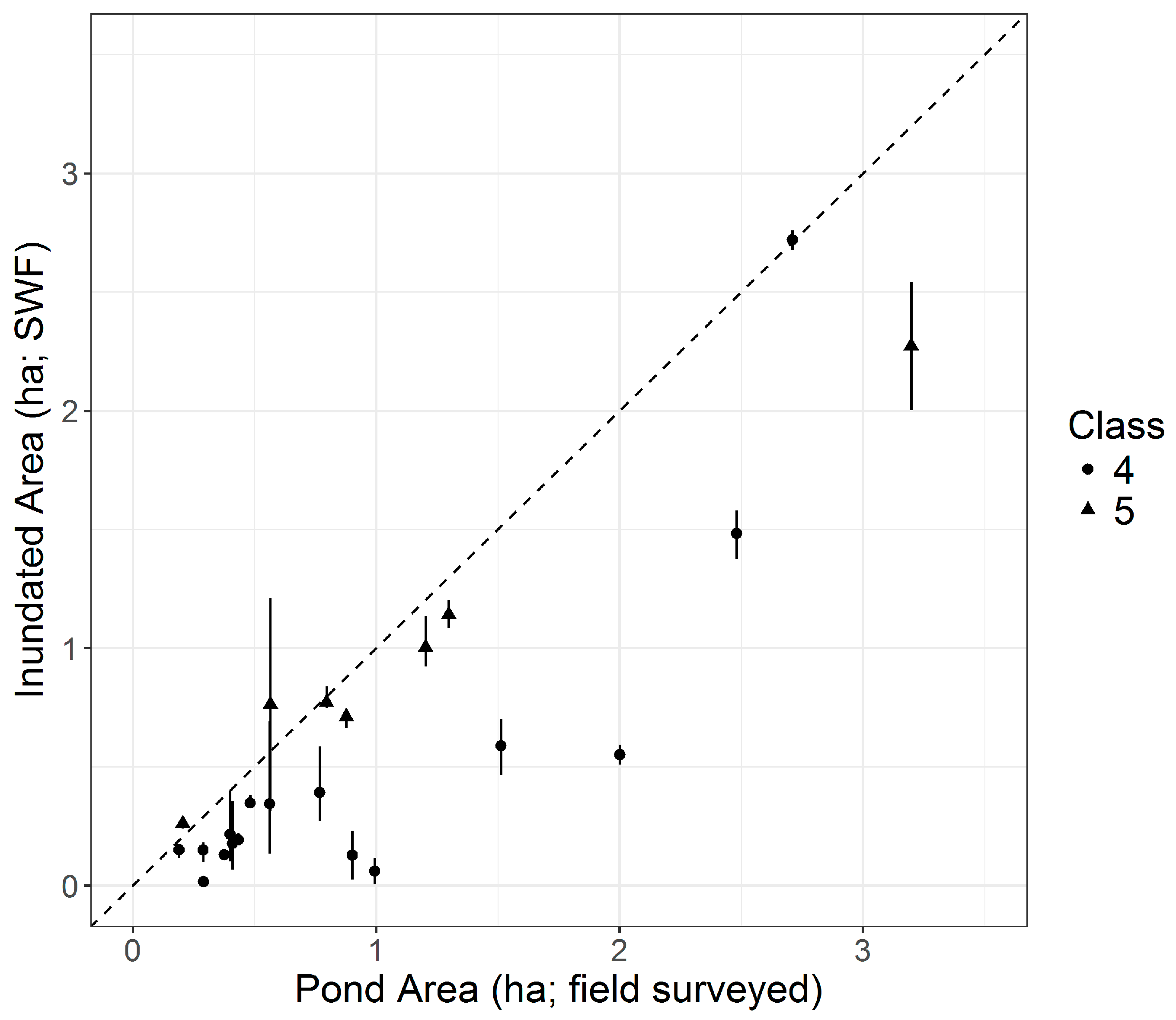
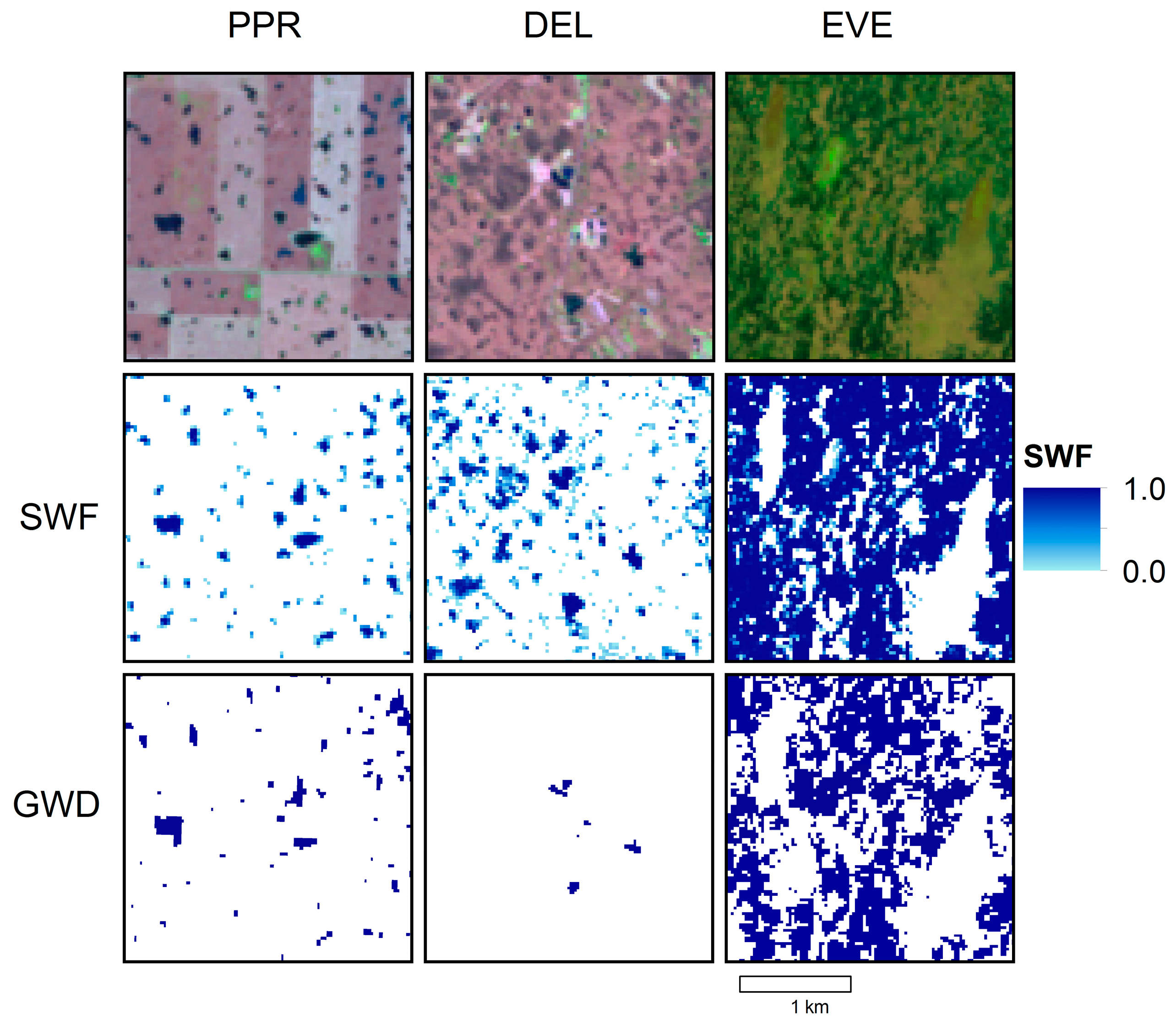
3.4.1. Prairie Pothole Region

For the Prairie Pothole Region site, we assessed the algorithm performance by comparing inundated area derived from Landsat SWF with field measured wetland area from four wetland sites surveyed on 25 May 2005, 27 May 2005, 1 June 2005, and 9 June 2005, respectively. Climate conditions in 2005 at the study sites, inferred from precipitation and potential evapotranspiration measurements, were near average conditions measured during the period from 1991 to 2016 [78]. Selected wetlands within each site were surveyed using a GPS receiver. Each of the surveyed wetlands was assigned a class label from 1 to 5 based on hydrological and vegetation characteristics [48]. We included only wetland classes known to be permanently inundated (classes 4 and 5) in our analysis, since wetlands belonging to other ephemeral classes were mapped based on potential rather than actual inundation.

To derive inundated area from SWF, we identified clusters of contiguous pixels using an 8-member (“Queen rule”) definition. We assumed that each cluster represented individual wetlands. We computed the inundated area (IA) of each cluster overlapping field-surveyed polygons as:

$$IA=0.09X{\displaystyle \sum }_i^{n}SW{F}_i$$

(1)

for each cluster comprised of $n$ pixels, each pixel representing an estimate of SWF and covering a surface area of 0.09 ha. Pixels with an SWF of 1 thus represented an inundated area of 0.09 ha, pixels with an SWF of 0.5 an inundated area of 0.045 ha, and so on. Since Landsat overpass times coincident with field sampling dates were rare, we estimated inundated area from Landsat SWF data through linear interpolation between the nearest SWF clusters preceding and following the field sampling dates for each wetland polygon. For estimates preceding the field sample dates, average lag times were found to be 13.1 days, with a maximum of 20 days and minimum of 5 days. For estimates following the field sample dates, average lag times were found to be 14.4 days, with a maximum of 27 days and minimum of 11 days.

The root mean square error (RMSE) of our estimates of inundated area compared to field surveyed wetlands was then computed as:

$$RMSE=\sqrt{\frac{\sum {({\hat{y}}_i-y_i)}^2}{n}}$$

(2)

where $\hat{y}$ and $y$ are the estimated and reference (measured) values, respectively, over $n$ samples. To allow for comparison with results from the Delmarva and Everglades sites, which were assessed using SWF directly (i.e., ranging from 0 to 1 as described below), we also computed the normalized RMSE (nRMSE) as:

$$nRMSE=\frac{RMSE}{y_{max}-y_{min}}$$

(3)

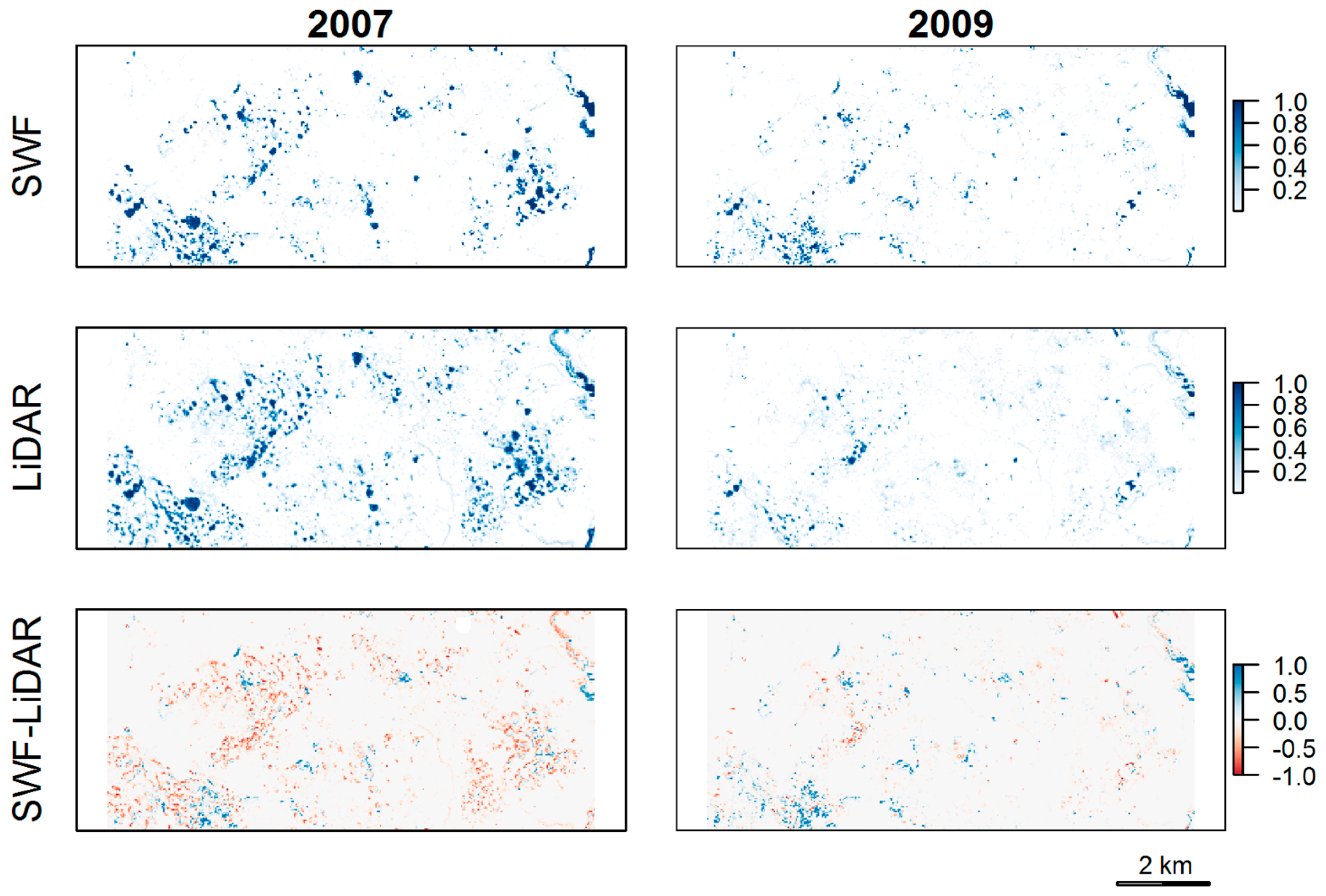
3.4.2. Delmarva Peninsula

For the Delmarva site, LiDAR intensity data (1-m resolution) over forested wetland sites in the Choptank watershed were used to derive reference SWF at 30-m resolution [41,61,79]. Intensity thresholds indicating inundation were calibrated using inundation observations from field-based transects [61]. LiDAR datasets were acquired in the spring seasons of 2007 and 2009, representing a relatively wet and dry year, respectively. These datasets are described in more detail in [41,79]. Since SWF is already scaled to a fraction between 0 and 1, the RMSE described in Equation (2) is already considered normalized and was used to test the accuracy of SWF estimates.

3.4.3. Everglades

For the Everglades site, we used a continuous record of water depth measurements from the Everglades Depth Estimation Network (EDEN) [80] to assess the performance of the SWF algorithm over time. EDEN is comprised of 313 individual gages spread over the Everglades, where water stage has been logged at an hourly basis from as early as 1999 until present. We took the median daily water depths at each site, measured in feet above a the North American Vertical Datum of 1988 (NADV88), and converted these daily water depths to millimeters (mm) above ground surface by subtracting the minimum elevation within plots with an approximately 10-m radius surrounding the gages. Gage readings were sampled for all dates where Landsat images were available between 1 January 2000 and 1 July 2016.

We implemented a “DEM flooding” method adapted from [81] to generate reference SWF for a subset of the Everglades water depth gages (Figure 3). DEM (Digital Elevation Model) flooding infers the water table height within a local window surrounding a water depth gage. Based on the assumption that there is no hydraulic gradient in the area covered by the local window, the water surface surrounding the gage is effectively the same height as the reading taken from the gage at any given time, creating a time-specific water/non-water mask within the window at the spatial resolution of the original DEM (Figure 3B). Given that the DEM spatial resolution is finer than that of the target reference data, this water/non-water mask was resampled to the target resolution using bilinear resampling to obtain an independent estimate of SWF at the same resolution as the dataset being assessed (Figure 3C).

We used a 5-foot (~1.5-m) resolution DEM produced for Miami-Dade County by the South Florida Water Management District (SFWMD) [82]. The DEM was produced using airborne LiDAR data from the 2007 Florida Division of Emergency Management Statewide Coastal LiDAR project (acquired between July 2007 and April 2008), and has a vertical accuracy of 0.61 feet (~0.19 m), consolidated from RMSE estimates across all land cover types. We visually assessed all of the available gages and removed gages with one or more of the following characteristics: (1) no overlap with the local DEM; (2) elevation data contained noise or anomalies (e.g., linear features from adjacent LiDAR flight paths); or (3) gage situated adjacent to a watercourse or reservoir which would affect our assumption of no hydraulic gradient described above. Using the remaining 17 gages (summarized in

Table 5. Location of Everglades water depth gages (decimal degrees, WGS 1984) and average ground elevation (above the North American Vertical Datum of 1988) at gage sites used in this study.

EDEN Station Name	Longitude	Latitude	Average Ground Elevation (ft)	Average Ground Elevation (m)
ANGEL	−80.5417	25.6226	4.73	1.442
C111	−80.5200	25.2944	0.02	0.006
CP	−80.7039	25.2275	−1.49	−0.454
E112	−80.6097	25.4239	2.43	0.741
E146	−80.6663	25.2526	−0.46	−0.290
EP1R	−80.4531	25.2875	−0.88	−0.268
EPSW	−80.5081	25.2714	−0.21	−0.064
EVER4	−80.5467	25.3388	−0.5	−0.152
EVER6	−80.5114	25.2969	0.34	0.104
G-3437	−80.5671	25.5670	5.27	1.606
G-3626	−80.5113	25.6186	5.75	1.753
G-3628	−80.5347	25.5941	5.55	1.692
G-3761	−80.4335	25.8417	3.25	0.991
NCL	−80.7444	25.2425	−1.29	−0.393
NTS1	−80.5928	25.4367	3.32	0.884
NTS10	−80.6050	25.4603	3.89	1.155
R3110	−80.6261	25.4461	3.65	1.113

), we employed the DEM flooding method to 500-m by 500-m windows surrounding each gage and produced 30-m resolution reference SWF data for all dates where both gage depth readings and Landsat data were available. We chose a smaller window than that employed by Cazals et al. (2016) [81] to reduce uncertainties arising from heterogeneity in the local water table surrounding the gages. After rejecting any samples with masked data from clouds or Scan Line Corrector (SLC) gaps from the Landsat imagery, 2815 individual SWF samples across the 17 gage sites were available for comparison.

4. Results

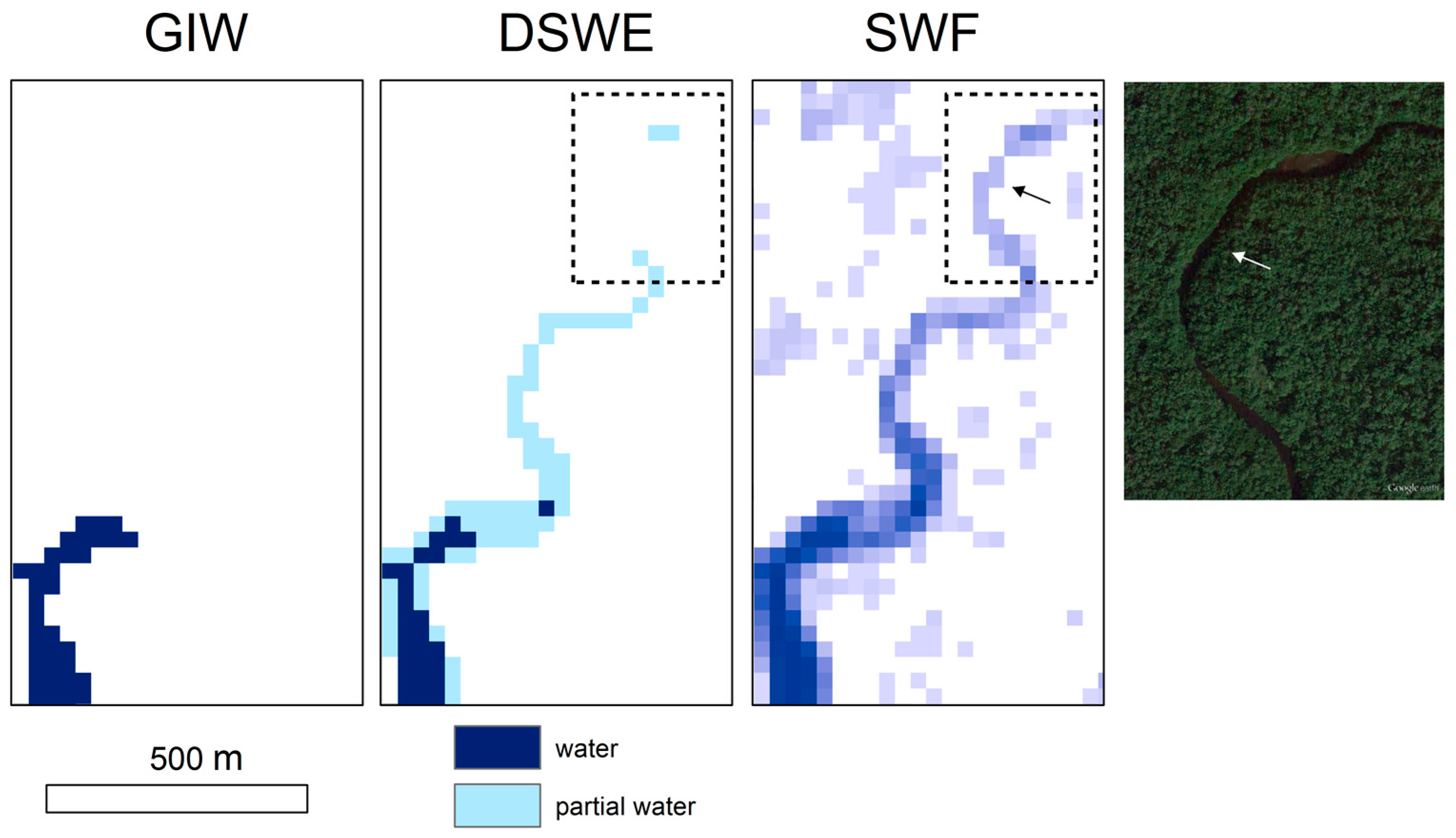
4.1. Spatial Assessment

The accuracy estimates for each site are summarized in

Table 6. Accuracy of surface water extent estimates at each of the three sites.

Dataset	Measure	Value	n
Prairie Pothole Region
Class 4 ponds	RMSE	0.61 ha	16
	nRMSE	0.23
Class 5 ponds	RMSE	0.38 ha	7
	nRMSE	0.18
All	RMSE	0.55 ha	23
	nRMSE	0.18
Delmarva
LiDAR-2007	nRMSE	0.15	--
LiDAR-2009	nRMSE	0.11	--
Everglades
Gage sites	median RMSE	0.19	2815

. In the Prairie Pothole Region, the absolute RMSE was estimated at 0.55 ha, and the normalized RMSE was estimated at 0.18 for class 4 and 5 ponds. Class 4 ponds (RMSE = 0.61 ha; nRMSE = 0.23) had lower accuracy than class 5 ponds (RMSE = 0.38 ha; nRMSE = 0.18). The errors in SWF estimates were largely due to a negative bias, where area estimates were usually lower than field measurements (Figure 4). In the Delmarva Peninsula, the nRMSE was estimated at 0.15 for the 2007 LiDAR data (wet spring) and 0.11 for the 2009 LiDAR data (dry spring). Landsat-derived SWF largely underestimated inundation in the 2007 dataset, as is evident from the red pixels in Figure 5 (bottom left panel). Most of the underestimated inundation was found around the fringes of forested wetland features. In the Everglades, the median nRMSE over 2815 reference SWF estimates (17 gage sites with an average of 166 sampled dates per sub-site) was found to be 0.19.

To further assess the spatial representation of inundation using our method, we performed both a quantitative and qualitative comparison of the SWF results from our algorithm to that of the recently published Global Surface Water dataset (GWD) [14]. For this comparison, we used the “maximum extent” layer of the GWD dataset, defined in [14] as any pixel to have ever been mapped as water in the 32-year period of the Landsat archive. First, to quantitatively assess the ability of SWF to capture small wetlands compared to GWD, we used each dataset to independently identify inundated wetland features for a single Landsat path row (37/25) over the Prairie Pothole Region site. Wetlands from the SWF dataset were detected by identifying clusters of pixels in which the median SWF, computed from all Landsat 5 TM images acquired between April to September 2005 inclusive (nine images in total), was greater than zero. Wetlands from the GWD dataset were detected using the maximum inundated extent layer, similarly identifying clusters of pixels assigned a “water” label. The cumulative distribution of individual inundated wetlands is shown in Figure 6. Large differences in inundation detection capabilities between the two datasets are especially evident for sub-hectare wetlands. The GWD dataset was able to identify 55,113 wetlands, whereas the median SWF dataset identified 249,097 wetlands, an increase by a factor of 4.5.

A qualitative comparison between SWF (computed from single Landsat acquisitions) and GWD is shown in Figure 7. In all three sites, SWF captured more inundated features than that of the maximum-extent Global Surface Water data. Some wetlands on the order of one to two Landsat pixels (0.1–0.2 ha) were captured by the Global Surface Water data in the Prairie Pothole Region (Figure 7, left panels). However, SWF was able to capture very small wetlands with area below that of a single Landsat pixel (i.e., area < 0.1 ha and SWF < 1.0). Water bodies in the forested wetland site in Delmarva shown in Figure 7 (middle panels) were largely omitted by the Global Surface Water dataset but captured by the SWF product. Inundation in the wetland complexes of the Everglades was evident in both datasets, but SWF gave a more complete representation of inundation, including both open water and areas with flooded vegetation.

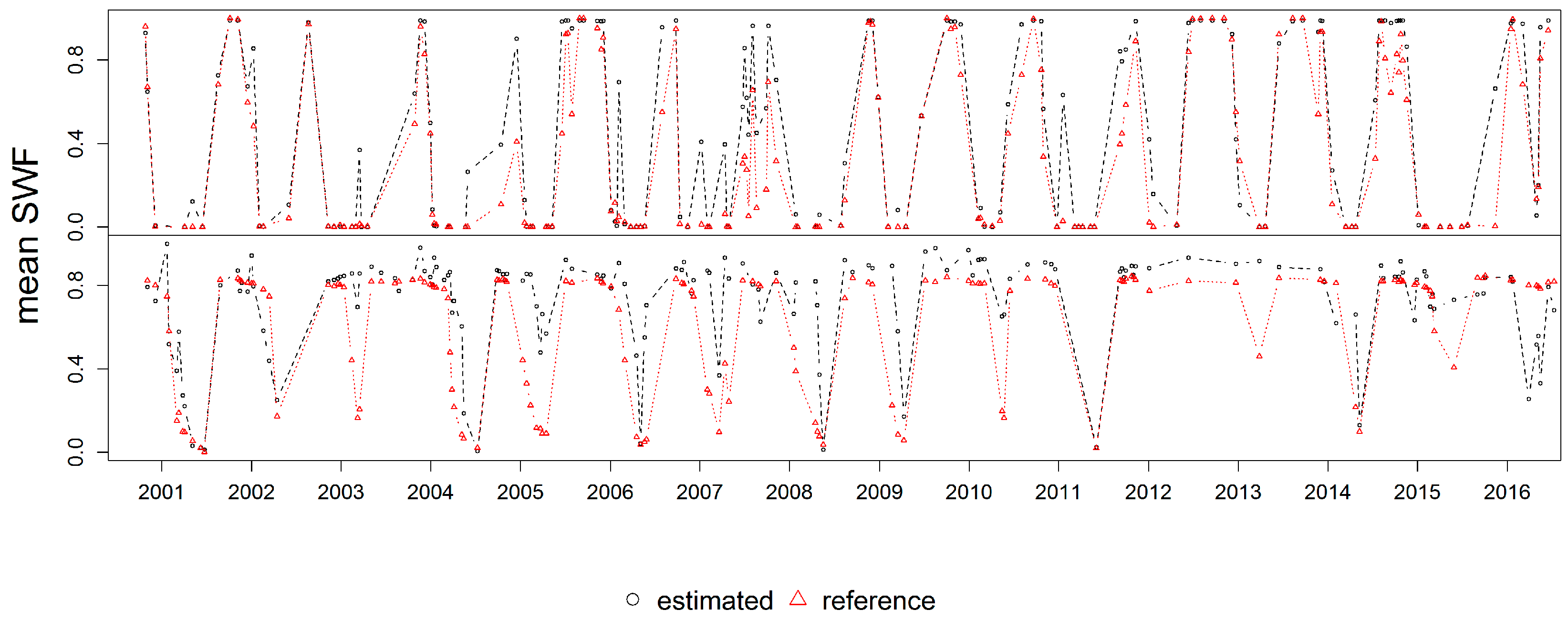
4.2. Temporal Assessment

To assess the performance of the SWF algorithm over a range of conditions, we applied the algorithm to all available Landsat images over the Everglades and compared the results to reference SWF from the 17 gage sites described above for all time steps in which both estimated and reference SWF were available. Temporal profiles of both estimated and reference SWF are shown in Figure 8 for two of these gage sites. Reference and estimated SWF followed expected seasonal patterns, with a drying trend in the spring and an increase in inundation in the autumn and winter seasons. However, SWF was frequently over-estimated in gage sites where partial inundation prevailed, as is evident in several years in the top panel (e.g., late 2004, 2007 and late 2011) and most years of the bottom panel of Figure 8. Additionally, several “spikes” in the time series of estimated SWF in the top panel of Figure 8 indicate over-estimates likely caused by commission errors.

5. Discussion

5.1. Automation and Scalability

A fully automated and scalable algorithm was developed for the quantification of SWF over diverse wetland types, with the eventual aim of developing large-area dynamic inundation data products. This work builds on a range of site-specific methods that have been developed in recent years to track surface water inundation from Landsat data at a sub-pixel scale [37,41,42,83,84,85]. These supervised methods are generally capable of capturing inundation characteristics of specific wetland ecosystems, but depend on external training data, which limits their applicability to continental to global-scale analysis. In contrast, unsupervised methods to classify inundation types [28] or quantify SWF [37] have shown promise in rapid assessment of wetland inundation. Our study builds upon these advances by demonstrating the potential of unsupervised SWF quantification methods to quantify SWF over a variety of wetland types. Avoiding the time-consuming task of gathering training data, our algorithm generates a SWF estimate over an entire Landsat scene in under eight minutes (running on 10 parallel processes). Operational Earth observation satellite missions with open data distribution policies [15,86] combined with rapid advances in cloud computing for geospatial data processing [87] will allow for the application of our algorithm to continental to global scale analysis of wetland inundation at high temporal resolution. Validation strategies for these products will need to take into account the challenges of validating sub-pixel water fraction over areas where in situ inundation data are not available. Efforts to consolidate very high resolution imagery (often with sub-meter resolution), such as the continued acquisition of commercial imagery by the National Geospatial-Intelligence Agency (NGA) since 2003 [88], will be key in producing large-area SWF products and forming comprehensive validation plans.

5.2. Strengths and Limitations

Most existing regional to global inundation products are based on classified water surfaces and often omit wetland inundation features in the presence of other reflective features such as flooded vegetation. The results presented in this study represent a significant step forward towards the quantification of wetland inundation dynamics over large heterogeneous wetlands. Below, we discuss the strengths and weaknesses of our approach in the contexts of the validation and comparison with existing global-scale surface water data products for each of the three sites featured in this study.

5.2.1 Small Hemispherical Wetlands

Very small hemispherical water bodies commonly found in the Prairie Pothole Region and other wetland-dominated landscapes such as the thermokarst region of northern Canada and Alaska [37], are commonly omitted by optical-based classifiers, especially when their size is less than the pixel size of the source imagery [25,37]. Very small water bodies are extremely abundant in the Prairie Pothole Region, and their omission in models describing regional to global phenomenon (e.g., climate) has significant implications [89,90]. While an RMSE of 0.55 ha in the Prairie Pothole Region suggests an effective detection limit of 0.5 ha, the inundated area comparison shown in Figure 4, the cumulative inundated wetland frequency shown in Figure 6 and the visual example shown in Figure 7 (left panel) all suggest that our SWF algorithm does indeed detect much smaller water bodies, with several single-pixel features with SWF less than 1.0 indicating the presence of inundated ponds with surface area well below that limit. Therefore, the RMSE reported for this site should be a conservative estimate, as very small wetlands were likely not fully represented in the reference dataset. We expect that an in-depth analysis of inundation over a larger range of pond sizes and classes would reveal higher sensitivity of our algorithm than what we have shown in this study.

5.2.2. Forested Depressional Wetlands

Detection of sub-canopy inundation in forested wetlands using optical satellite imagery is particularly difficult, and virtually impossible during leaf-on periods [41,44]. Monitoring sub-canopy inundation using synthetic aperture radar (SAR) data, on the other hand, has shown some promise, especially in the case of longer wavelength data (e.g., L-band) [79]. In this study, we detected sub-canopy inundation with RMSEs of 0.15 and 0.11 during leaf-off in 2007 and 2009, respectively. While these errors are higher than those reported in a recent study quantifying SWF using Landsat imagery over the Delmarva Peninsula [44], a number of differences should be considered in this comparison. First, we considered forested wetlands in estimating algorithm accuracy, whereas Jin et al. (2017) [44] based their accuracy on open waters, which was not the focus of this study. Second, our algorithm does not use any local training data, and as such we expect that our results will have lower accuracies than most locally-trained algorithms, such as a similar product reported in [41]. A comparison of our results over forested wetlands with the Global Surface Water dataset [14] reveals that the Global Surface Water dataset failed to map most of the under-canopy inundation, whereas the SWF algorithm developed in this study is sensitive to a much larger proportion of sub-canopy inundation (Figure 7, center top and bottom).

5.2.3. Large Heterogeneously Inundated Wetlands

We included the Everglades site in this study to demonstrate the applicability of our algorithm over large, heterogeneously inundated surfaces, in contrast to the discrete hemispherical water bodies and depressional wetlands that dominate the Prairie Pothole wetlands and Delmarva forested wetlands. Although an overall RMSE of 0.19 across more than 2000 depth gage measurements collected over nearly two decades indicates that our algorithm is accurate, several important sources of errors and uncertainties warrant consideration. First, the results of the DEM-flooding method utilized in this study are affected by the facts that the LiDAR data used to derive the DEM would not have fully penetrated the vegetation canopy to the soil surface and that water may have been present on the surface at the time of data collection. Both of these factors are expected to introduce errors in the derived reference SWF over all dates. Second, while we did not perform an in-depth analysis of error sources, recent work comparing the DSWE product with normalized difference vegetation index (NDVI) time series has shown that inundation detection errors are largely a function of vegetation cover [28]. Given the reliance of our SWF estimates to the input DSWE data product, we expect that these errors propagate to the final SWF estimate as well. Additionally, a multi-temporal demonstration of our algorithm (Figure 8) shows that our algorithm consistently over-estimated SWF during periods where partial inundation was apparent from the reference dataset, which is likely a limitation in our algorithm’s ability to adequately model SWF in these types of wetlands. While the aggregation step in our algorithm succeeded in generating reliable training data in areas with open water bodies (e.g., the Prairie Pothole Region and Delmarva), large contiguous areas of partial inundation (as in the Everglades) generate uncertainties in SWF, which propagate to the final SWF estimate in areas where image pixels are predominantly characterized by partial water. Further research will explore alternate approaches to automatically deriving SWF training data without relying on the assumption of an initial SWF in known partial water pixels.

Despite these limitations of the algorithm, more inundated area across the Everglades site was mapped than is commonly seen in Global Surface Water datasets. As in the other sites described above, a comparison with the Global Surface Water dataset [14] shows that detecting inundation at the sub-pixel scale allows for a better representation of inundation over such large heterogeneous wetlands, allowing for discrimination between inundated surfaces and tree islands (non-inundated elliptical features in Figure 7, right top and bottom). It is important to note that the SWF estimate (top) is a “snapshot” at a given time, whereas the Global Surface Water dataset (bottom) represents the maximum inundation extent over a multi-decadal time series dataset [14]. As demonstrated in Figure 8, inundation varies rapidly in response to weather variability, suggesting that the Global Surface Water dataset gives a very conservative representation of inundation over this site. Conservative estimates of water extent in global datasets frequently give rise to the omission of large heterogeneously inundated landscapes, especially in the case of large wetland complexes such as the Everglades [28]. Work is currently underway to reduce omission errors in the DSWE product used to initiate SWF processing.

5.3. Potential Applications of SWF

The sub-pixel representation of inundation in wetlands is necessary for a more robust understanding of hydrological, biogeochemical and ecological processes in these systems [37]. Global inventories of small water bodies have revealed major discrepancies in global water extent estimates when small water bodies (with area <1 km²) are not considered [89,91]. Our analysis revealed that using a sub-pixel approach to detect wetland inundation allowed for a greater than fourfold increase in sensitivity compared to a state-of-the-art global inundation product [14]. Based on this observation, we conclude that surface inundation algorithms that rely on medium spatial resolution data like Landsat or Sentinel-2 must be designed to detect surface water at sub-pixels scales to be able to overcome the omissions affecting current wetlands and small water bodies.

This enhancement will in turn help to improve understanding of the influence of small water bodies on both local and global ecosystem processes. The importance of inland waters—particularly small lakes and ponds—in carbon cycling has come to light in recent years with the realization that wetlands and water bodies are not simply “vehicles” for transporting carbon through the landscape, but act as important carbon sources and sinks [90]. With a relative molecular radiative forcing upwards of 20 times that of carbon dioxide [92] and atmospheric concentrations likely higher than any time in the past 650,000 years [93], methane cycling in wetlands is of particular concern to the climate research community. Wetlands can act as methane sources or sinks depending on various factors including vegetation, climate and hydroperiod [94] and have been identified as the largest net methane source in some parts of the world [95]. Lack of reliable information on wetlands is therefore responsible for a large share of the uncertainties in global methane models [96]. The automation made possible with the algorithm described in this paper will allow for the quantification of inundation dynamics at continental to global scales, thus helping to address uncertainties in the role of wetlands and surface inundation in global carbon cycles.

Another aspect of wetland ecosystems to which SWF will contribute is a more complete understanding of hydrologic connectivity, which mediates the transport of nutrients and organisms throughout watersheds [97]. Characterizing surface water connectivity associated with wetland ecosystems is critical to understanding these watershed-scale processes. In this study, we present several examples that demonstrate how the quantification of inundation using SWF allowed for better representation of connected inundated features than with classified water products. One such example in a forested stream in the southwestern Everglades is demonstrated in Figure 9, in which the Global Inland Water product [18], DSWE [28] and SWF from this study are compared. Depicting watercourses using continuous fields (SWF) instead of a binary classification (as in the Global Inland Water product) allowed for detection of features well below the sensor pixel size, and therefore a more complete representation of the watercourse. The accurate representation of hydrologic connections and their dynamics will help to improve models describing hydrologic controls on biogeochemistry and biodiversity, with implications for management and policy in wetland systems [98,99].

6. Conclusions

The accurate characterization of hydrology in wetlands is needed to understand their function across landscapes. While Earth observation satellites provide excellent opportunities for mapping and quantifying wetland inundation, currently available surface water datasets still fail to adequately represent inundation dynamics in complex wetlands. We designed an unsupervised regression algorithm, adapted from several existing methods [28,37], to quantify sub-pixel water fraction from Landsat imagery. We estimated normalized RMSE’s ranging from 0.11 to 0.19 using in situ or fine resolution airborne data collected over three wetland sites across North America. Our algorithm was also shown to be highly sensitive to inundation in sub-hectare water bodies, forested wetlands and wetlands with emergent vegetation, when compared to existing dynamic surface water products [14]. This enhanced sensitivity demonstrates that optical satellite imagery can be used to effectively monitor surface hydrology in wetland ecosystems representing a range of hydrologic and vegetation characteristics. Additionally, the fact that our algorithm is fully automated allows for rapid quantification of inundation dynamics over time by applying it to time series of optical imagery. Taken together with the enhancements in sensitivity, this ability presents an opportunity to study wetland inundation dynamics over broad spatial and temporal scales with higher detail than has previously been possible.

A number of issues will need to be explored in future research to enable the spatial and temporal scaling of the work presented here. First, errors of commission described here and typically encountered in optical surface water detection algorithms should be addressed using additional information. For example, terrain shadows are commonly mis-classified as surface water, necessitating the use of terrain-related information to correct for these effects [28]. Second, the temporal resolution of Landsat observations, while sufficient for quantifying seasonal inundation dynamics in some ecosystems, will result in substantial uncertainties in the quantification of temporal dynamics (e.g., hydroperiod) in other wetland ecosystems. To this end, adapting our algorithm to allow its application to data from the recently launched Sentinel-2A and -2B optical sensors could result in a threefold increase in the temporal frequency of observations [100]. Finally, fusion of surface inundation data based on optical observations with those based on SAR data (e.g., from the recently launched Sentinel-1 satellites) will be necessary to further increase the temporal resolution of these data in areas where persistent cloud cover precludes regular inundation monitoring using optical data streams alone. For example, interferometric SAR (InSAR) methods have been shown to be highly effective in monitoring inundation dynamics over time [101]. The integration of optical and SAR data will also benefit from the ability of SAR data to detect sub-canopy inundation in forested wetlands under a wider range of phenology conditions than optical data [79,102].

References

1. DeGroot, R.; Stuip, M.; Finlayson, M.; Davidson, N. Valuing Wetlands Guidance for Valuing the Benefits Derived from Wetland Ecosystem Services; Ramsar Convention Secretariat: Gland, Switzerland; Secretariat of the Convention on Biological Diversity: Montreal, QC, Canada, 2006. [Google Scholar]
2. Clare, S.; Creed, I.F. Tracking wetland loss to improve evidence-based wetland policy learning and decision making. Wetl. Ecol. Manag. 2014, 22, 235–245. [Google Scholar] [CrossRef]
3. Kingsford, R.T.; Basset, A.; Jackson, L. Wetlands: Conservation’s poor cousins. Aquat. Conserv. Mar. Freshw. Ecosyst. 2016, 26, 892–916. [Google Scholar] [CrossRef]
4. Green, A.J.; Alcorlo, P.; Peeters, E.T.; Morris, E.P.; Espinar, J.L.; Bravo-Utrera, M.A.; Bustamante, J.; Díaz-Delgado, R.; Koelmans, A.A.; Mateo, R.; et al. Creating a safe operating space for wetlands in a changing climate. Front. Ecol. Environ. 2017, 15, 99–107. [Google Scholar] [CrossRef]
5. Sass, G.Z.; Creed, I.F. Characterizing hydrodynamics on boreal landscapes using archived synthetic aperture radar imagery. Hydrol. Process. 2008, 22, 1687–1699. [Google Scholar] [CrossRef]
6. Hayashi, M.; van der Kamp, G.; Rosenberry, D.O. Hydrology of Prairie Wetlands: Understanding the Integrated Surface-Water and Groundwater Processes. Wetlands 2016, 36, 237–254. [Google Scholar] [CrossRef]
7. Creed, I.F.; Beall, F.D.; Clair, T.A.; Dillon, P.J.; Hesslein, R.H. Predicting export of dissolved organic carbon from forested catchments in glaciated landscapes with shallow soils. Glob. Biogeochem. Cycles 2008, 22. [Google Scholar] [CrossRef]
8. Creed, I.F.; Beall, F.D. Distributed topographic indicators for predicting nitrogen export from headwater catchments. Water Resour. Res. 2009, 45. [Google Scholar] [CrossRef]
9. Mengistu, S.G.; Creed, I.F.; Webster, K.L.; Enanga, E.; Beall, F.D. Searching for similarity in topographic controls on carbon, nitrogen and phosphorus export from forested headwater catchments. Hydrol. Process. 2014, 28, 3201–3216. [Google Scholar] [CrossRef]
10. Saunois, M.; Bousquet, P.; Poulter, B.; Peregon, A.; Ciais, P.; Canadell, J.G.; Dlugokencky, E.J.; Etiope, G.; Bastviken, D.; Houweling, S.; et al. The Global Methane Budget: 2000–2012. Earth Syst. Sci. Data Discuss. 2016, 8, 697–751. [Google Scholar] [CrossRef]
11. Meng, L.; Hess, P.G.M.; Mahowald, N.M.; Yavitt, J.B.; Riley, W.J.; Subin, Z.M.; Lawrence, D.M.; Swenson, S.C.; Jauhiainen, J.; Fuka, D.R. Sensitivity of wetland methane emissions to model assumptions: Application and model testing against site observations. Biogeosciences 2012, 9, 2793–2819. [Google Scholar] [CrossRef]
12. Watts, J.D.; Kimball, J.S.; Bartsch, A.; McDonald, K.C. Surface water inundation in the boreal-Arctic: Potential impacts on regional methane emissions. Environ. Res. Lett. 2014, 9. [Google Scholar] [CrossRef]
13. Vörösmarty, C.J.; McIntyre, P.B.; Gessner, M.O.; Dudgeon, D.; Prusevich, A.; Green, P.; Glidden, S.; Bunn, S.E.; Sullivan, C.A.; Liermann, C.R.; et al. Global threats to human water security and river biodiversity. Nature 2010, 467, 555–561. [Google Scholar] [CrossRef] [PubMed]
14. Pekel, J.-F.; Cottam, A.; Gorelick, N.; Belward, A.S. High-resolution mapping of global surface water and its long-term changes. Nature 2016, 1–19. [Google Scholar] [CrossRef] [PubMed]
15. Wulder, M.A.; Masek, J.G.; Cohen, W.B.; Loveland, T.R.; Woodcock, C.E. Opening the archive: How free data has enabled the science and monitoring promise of Landsat. Remote Sens. Environ. 2012, 122, 2–10. [Google Scholar] [CrossRef]
16. Torres, R.; Snoeij, P.; Geudtner, D.; Bibby, D.; Davidson, M.; Attema, E.; Potin, P.; Rommen, B.; Floury, N.; Brown, M.; et al. GMES Sentinel-1 mission. Remote Sens. Environ. 2012, 120, 9–24. [Google Scholar] [CrossRef]
17. Drusch, M.; Del Bello, U.; Carlier, S.; Colin, O.; Fernandez, V.; Gascon, F.; Hoersch, B.; Isola, C.; Laberinti, P.; Martimort, P.; et al. Sentinel-2: ESA’s Optical High-Resolution Mission for GMES Operational Services. Remote Sens. Environ. 2012, 120, 25–36. [Google Scholar] [CrossRef]
18. Feng, M.; Sexton, J.O.; Channan, S.; Townshend, J.R. A global, high-resolution (30-m) inland water body dataset for 2000: First results of a topographic–spectral classification algorithm. Int. J. Digit. Earth 2015, 8947, 1–21. [Google Scholar] [CrossRef]
19. Yamazaki, D.; Trigg, M.A.; Ikeshima, D. Development of a global ~90 m water body map using multi-temporal Landsat images. Remote Sens. Environ. 2015, 171, 337–351. [Google Scholar] [CrossRef] [Green Version]
20. Carroll, M.; Townshend, J.R.; DiMiceli, C.M.; Noojipady, P.; Sohlberg, R.A. A new global raster water mask at 250 m resolution. Int. J. Digit. Earth 2009, 2, 291–308. [Google Scholar] [CrossRef]
21. Schroeder, R.; McDonald, K.; Chapman, B.; Jensen, K.; Podest, E.; Tessler, Z.; Bohn, T.; Zimmermann, R. Development and Evaluation of a Multi-Year Fractional Surface Water Data Set Derived from Active/Passive Microwave Remote Sensing Data. Remote Sens. 2015, 7, 16688–16732. [Google Scholar] [CrossRef]
22. Fluet-Chouinard, E.; Lehner, B.; Rebelo, L.M.; Papa, F.; Hamilton, S.K. Development of a global inundation map at high spatial resolution from topographic downscaling of coarse-scale remote sensing data. Remote Sens. Environ. 2015, 158, 348–361. [Google Scholar] [CrossRef]
23. Verpoorter, C.; Kutser, T.; Tranvik, L.J. Automated mapping of water bodies using Landsat multispectral data. Limnol. Oceanogr. Methods 2012, 10, 1037–1050. [Google Scholar] [CrossRef]
24. Watts, J.D.; Kimball, J.S.; Jones, L.A.; Schroeder, R.; McDonald, K.C. Satellite Microwave remote sensing of contrasting surface water inundation changes within the Arctic-Boreal Region. Remote Sens. Environ. 2012, 127, 223–236. [Google Scholar] [CrossRef]
25. Carroll, M.; Wooten, M.; DiMiceli, C.; Sohlberg, R.; Kelly, M. Quantifying Surface Water Dynamics at 30 Meter Spatial Resolution in the North American High Northern Latitudes 1991–2011. Remote Sens. 2016, 8. [Google Scholar] [CrossRef]
26. Mueller, N.; Lewis, A.; Roberts, D.; Ring, S.; Melrose, R.; Sixsmith, J.; Lymburner, L.; McIntyre, A.; Tan, P.; Curnow, S.; Ip, A. Water observations from space: Mapping surface water from 25 years of Landsat imagery across Australia. Remote Sens. Environ. 2016, 174, 341–352. [Google Scholar] [CrossRef]
27. Lehner, B.; Döll, P. Development and validation of a global database of lakes, reservoirs and wetlands. J. Hydrol. 2004, 296, 1–22. [Google Scholar] [CrossRef]
28. Jones, J.W. Efficient wetland surface water detection and monitoring via landsat: Comparison with in situ data from the everglades depth estimation network. Remote Sens. 2015, 7, 12503–12538. [Google Scholar] [CrossRef]
29. McFeeters, S.K. The use of the Normalized Difference Water Index (NDWI) in the delineation of open water features. Int. J. Remote Sens. 1996, 17, 1425–1432. [Google Scholar] [CrossRef]
30. Xu, H. Modification of normalised difference water index (NDWI) to enhance open water features in remotely sensed imagery. Int. J. Remote Sens. 2006, 27, 3025–3033. [Google Scholar] [CrossRef]
31. Feyisa, G.L.; Meilby, H.; Fensholt, R.; Proud, S.R. Automated Water Extraction Index: A new technique for surface water mapping using Landsat imagery. Remote Sens. Environ. 2014, 140, 23–35. [Google Scholar] [CrossRef]
32. Xie, H.; Luo, X.; Xu, X.; Pan, H.; Tong, X. Automated Subpixel Surface Water Mapping from Heterogeneous Urban Environments Using Landsat 8 OLI Imagery. Remote Sens. 2016, 8. [Google Scholar] [CrossRef]
33. Tulbure, M.G.; Broich, M.; Stehman, S.V.; Kommareddy, A. Surface water extent dynamics from three decades of seasonally continuous Landsat time series at subcontinental scale in a semi-arid region. Remote Sens. Environ. 2016, 178, 142–157. [Google Scholar] [CrossRef]
34. Díaz-Delgado, R.; Aragonés, D.; Afán, I.; Bustamante, J. Long-Term Monitoring of the Flooding Regime and Hydroperiod of Doñana Marshes with Landsat Time Series (1974–2014). Remote Sens. 2016, 8. [Google Scholar] [CrossRef]
35. Tulbure, M.G.; Broich, M. Spatiotemporal dynamic of surface water bodies using Landsat time-series data from 1999 to 2011. ISPRS J. Photogramm. Remote Sens. 2013, 79, 44–52. [Google Scholar] [CrossRef]
36. Fisher, A.; Flood, N.; Danaher, T. Landsat water index methods for automated water classification in eastern Australia. Remote Sens. Environ. 2016, 175, 167–182. [Google Scholar] [CrossRef]
37. Rover, J.; Wylie, B.K.; Ji, L. A self-trained classification technique for producing 30 m percent-water maps from Landsat data. Int. J. Remote Sens. 2010, 31, 2197–2203. [Google Scholar] [CrossRef]
38. Vanderhoof, M.K.; Christensen, J.R.; Alexander, L.C. Patterns and drivers for wetland connections in the Prairie Pothole Region, United States. Wetl. Ecol. Manag. 2016, 25, 275–297. [Google Scholar] [CrossRef]
39. Sexton, J.O.; Song, X.-P.; Feng, M.; Noojipady, P.; Anand, A.; Huang, C.; Kim, D.-H.; Collins, K.M.; Channan, S.; Dimiceli, C.; et al. Global, 30-m resolution continuous fields of tree cover: Landsat-based rescaling of MODIS Vegetation Continuous Fields with lidar-based estimates of error. Int. J. Digit. Earth 2013, 8947. [Google Scholar] [CrossRef]
40. Sexton, J.O.; Song, X.-P.; Huang, C.; Channan, S.; Baker, M.E.; Townshend, J.R. Urban growth of the Washington, D.C.-Baltimore, MD metropolitan region from 1984 to 2010 by annual, Landsat-based estimates of impervious cover. Remote Sens. Environ. 2013, 129, 42–53. [Google Scholar] [CrossRef]
41. Huang, C.; Peng, Y.; Lang, M.W.; Yeo, I.Y.; McCarty, G. Wetland inundation mapping and change monitoring using Landsat and airborne LiDAR data. Remote Sens. Environ. 2014, 141, 231–242. [Google Scholar] [CrossRef]
42. Halabisky, M.; Moskal, L.M.; Gillespie, A.; Hannam, M. Reconstructing semi-arid wetland surface water dynamics through spectral mixture analysis of a time series of Landsat satellite images (1984–2011). Remote Sens. Environ. 2016, 177, 171–183. [Google Scholar] [CrossRef]
43. Li, S.; Sun, D.; Yu, Y.; Csiszar, I.; Stefanidis, A.; Goldberg, M.D. A new short-wave infrared (SWIR) method for quantitative water fraction derivation and evaluation with EOS/MODIS and landsat/TM data. IEEE Trans. Geosci. Remote Sens. 2013, 51, 1852–1862. [Google Scholar] [CrossRef]
44. Jin, H.; Huang, C.; Lang, M.W.; Yeo, I.-Y.; Stehman, S.V. Monitoring of wetland inundation dynamics in the Delmarva Peninsula using Landsat time-series imagery from 1985 to 2011. Remote Sens. Environ. 2017, 190, 26–41. [Google Scholar] [CrossRef]
45. Tiner, R.W. Geographically isolated wetlands of the United States. Wetlands 2003, 23, 494–516. [Google Scholar] [CrossRef]
46. Gala, T.S.; Aldred, D.A.; Carlyle, S.; Creed, I.F. Topographically based spatially averaging of SAR data improves performance of soil moisture models. Remote Sens. Environ. 2011, 115, 3507–3516. [Google Scholar] [CrossRef]
47. Clark, R.B.; Creed, I.F.; Sass, G.Z. Mapping hydrologically sensitive areas on the Boreal Plain: A multitemporal analysis of ERS synthetic aperture radar data. Int. J. Remote Sens. 2009, 30, 2619–2635. [Google Scholar] [CrossRef]
48. Stewart, R.E.; Kantrud, H.A. Vegetation of Prairie Potholes, North Dakota, in Relation to Quality of Water and Other Environmental Factors; U.S. Geological Survey: Reston, VA, USA, 1972; Volume 585.
49. Miller, B.A.; Crumpton, W.G.; van der Valk, A.G. Spatial Distribution of Historical Wetland Classes on the Des Moines Lobe, Iowa. Wetlands 2009, 29, 1146–1152. [Google Scholar] [CrossRef]
50. Van Meter, K.J.; Basu, N.B. Signatures of human impact: Size distributions and spatial organization of wetlands in the Prairie Pothole landscape. Ecol. Appl. 2015, 25, 451–465. [Google Scholar] [CrossRef] [PubMed]
51. Warner, B.G.; Asada, T. Knowledge Gaps and Challenges in Wetlands under Climate Change in Canada. In Climate Change and Managed Ecosystems; Bhatti, J.S., Lal, R., Apps, M.J., Price, M.A., Eds.; Taylor & Francis: Boca Raton, FL, USA, 2006; pp. 355–374. [Google Scholar]
52. Dahl, T.E. Status and Trends of Prairie Wetlands in the United States 2004 to 2009; U.S. Department of the Interior, Fish and Wildlife Service: Washington, DC, USA, 2014.
53. Serran, J.N.; Creed, I.F. New mapping techniques to estimate the preferential loss of small wetlands on prairie landscapes. Hydrol. Process. 2016, 30, 396–409. [Google Scholar] [CrossRef]
54. Creed, I.F.; Miller, J.; Aldred, D.; Adams, J.K.; Spitale, S.; Bourbonniere, R.A. Hydrologic profiling for greenhouse gas effluxes from natural grasslands in the prairie pothole region of Canada. J. Geophys. Res. Biogeosci. 2013, 118, 680–697. [Google Scholar] [CrossRef]
55. Marton, J.M.; Creed, I.F.; Lewis, D.B.; Lane, C.R.; Basu, N.B.; Cohen, M.J.; Craft, C.B. Geographically isolated wetlands are important biogeochemical reactors on the landscape. Bioscience 2015, 65, 408–418. [Google Scholar] [CrossRef]
56. Rains, M.C.; Leibowitz, S.G.; Cohen, M.J.; Creed, I.F.; Golden, H.E.; Jawitz, J.W.; Kalla, P.; Lane, C.R.; Lang, M.W.; Mclaughlin, D.L. Geographically isolated wetlands are part of the hydrological landscape. Hydrol. Process. 2016, 30, 153–160. [Google Scholar] [CrossRef]
57. Golden, H.; Creed, I.F.; Ali, G.; Basu, N.; Neff, B.; Rains, M.; McLaughlin, D.; Alexander, L.; Ameli, A.; Christensen, J.; et al. Scientific tools for integrating geographically isolated wetlands into land management decisions. Front. Ecol. Environ. 2017, in press. [Google Scholar]
58. Gleason, R.A.; Euliss, N.H.; Tangen, B.A.; Laubhan, M.K.; Browne, B.A. USDA conservation program and practice effects on wetland ecosystem services in the Prairie Pothole Region Source. Ecol. Appl. 2016, 21, S35–S81. [Google Scholar]
59. Badiou, P.; McDougal, R.; Pennock, D.; Clark, B. Greenhouse gas emissions and carbon sequestration potential in restored wetlands of the Canadian prairie pothole region. Wetl. Ecol. Manag. 2011, 19, 237–256. [Google Scholar] [CrossRef]
60. Puchniak Begley, A.J.; Gray, B.T.; Paszkowski, C.A. A comparison of restored and natural wetlands as habitat for birds in the Prairie Pothole Region of Saskatchewan, Canada. Raffles Bull. Zool. 2012, 173–187. [Google Scholar]
61. Lang, M.W.; McCarty, G.W. Lidar intensity for improved detection of inundation below the forest canopy. Wetlands 2009, 29, 1166–1178. [Google Scholar] [CrossRef]
62. Dahl, T.E. Wetlands Losses in the United States: 1780’s to 1980’s; Department of the Interior, Fish and Wildlife Service: Washington, DC, USA, 1990.
63. Fisher, T.R.; Benitez, J.A.; Lee, K.; Sutton, A.J. History of land cover change and biogeochemical impacts in the Choptank River basin in the mid-Atlantic region of the US. Int. J. Remote Sens. 2006, 27, 3683–3703. [Google Scholar] [CrossRef]
64. Fenstermacher, D.E.; Rabenhorst, M.C.; Lang, M.W.; McCarty, G.W.; Needelman, B.A. Carbon in Natural, Cultivated, and Restored Depressional Wetlands in the Mid-Atlantic Coastal Plain. J. Environ. Qual. 2016, 45, 743–750. [Google Scholar] [CrossRef] [PubMed]
65. Jones, J.W. Image and in situ data integration to derive sawgrass density for surface flow modelling in the Everglades, Florida, USA. Remote Sens. Hydrol. 2000, 2000, 507–512. [Google Scholar]
66. Jones, J.W.; Hall, A.; Smith, T.J.; Foster, A. Wetland fire scar monitoring using Landsat Archive data for the Everglades. Fire Ecol. 2013, 9, 133–150. [Google Scholar] [CrossRef]
67. Carter, V.; Rybicki, N.B.; Reel, J.T.; Ruhl, H.A.; Stewart, D.W.; Jones, J.W. Classification of vegetation for surface-water flow models in Taylor Slough, Everglades National Park. In Proceedings of the Third International Symposium on Ecohydraulics, Salt Lake City, UT, USA, 12–16 July 1999. [Google Scholar]
68. Sumner, D.M.; Jacobs, J.M. Utility of Penman-Monteith, Priestley-Taylor, reference evapotranspiration, and pan evaporation methods to estimate pasture evapotranspiration. J. Hydrol. 2005, 308, 81–104. [Google Scholar] [CrossRef]
69. Snyder, G.H.; Davidson, J.M. Everglades Agriculture: Past, Present and Future. In Everglades: The Ecosystem and Its Restoration; Davis, S.M., Ogden, J.C., Eds.; St. Lucie Press: Delray Beach, FL, USA, 1994; pp. 85–115. [Google Scholar]
70. USACOE Comprehensive Everglades Restoration Plan (CERP). Available online: http://www.saj.usace.army.mil/Portals/44/docs/FactSheets/CERP_FS_March2015_revised.pdf (accessed on 5 May 2017).
71. Masek, J.G.; Vermote, E.F.; Saleous, N.E.; Wolfe, R.; Hall, F.G.; Huemmrich, K.F.; Gao, F.; Kutler, J.; Lim, T.K. A landsat surface reflectance dataset for North America, 1990–2000. IEEE Geosci. Remote Sens. Lett. 2006, 3, 68–72. [Google Scholar] [CrossRef]
72. Vermote, E.; Justice, C.; Claverie, M.; Franch, B. Preliminary analysis of the performance of the Landsat 8/OLI land surface reflectance product. Remote Sens. Environ. 2016, 185, 46–56. [Google Scholar] [CrossRef]
73. Zhu, Z.; Woodcock, C.E. Automated cloud, cloud shadow, and snow detection in multitemporal Landsat data: An algorithm designed specifically for monitoring land cover change. Remote Sens. Environ. 2014, 152, 217–234. [Google Scholar] [CrossRef]
74. Zhu, Z.; Wang, S.; Woodcock, C.E. Improvement and expansion of the Fmask algorithm: Cloud, cloud shadow, and snow detection for Landsats 4–7, 8, and Sentinel 2 images. Remote Sens. Environ. 2015, 159, 269–277. [Google Scholar] [CrossRef]
75. Jones, J.W. The Dynamic Surface Water Extent (DSWE) Evaluation Strategy. In Proceedings of the European Geoscience Union Annual Meeting, Vienna, Austria, 23–28 April 2017. [Google Scholar]
76. Tucker, C.J. Red and photographic infrared linear combinations for monitoring vegetation. Remote Sens. Environ. 1979, 8, 127–150. [Google Scholar] [CrossRef]
77. Crist, E.P. A TM Tasseled Cap equivalent transformation for reflectance factor data. Remote Sens. Environ. 1985, 17, 301–306. [Google Scholar] [CrossRef]
78. Natural Resources Canada Regional, National and International Climate Modeling. Available online: https://cfs.nrcan.gc.ca/projects/3/2 (accessed on 11 July 2017).
79. Lang, M.W.; Kasischke, E.S.; Prince, S.D.; Pittman, K.W. Assessment of C-band synthetic aperture radar data for mapping and monitoring Coastal Plain forested wetlands in the Mid-Atlantic Region, U.S.A. Remote Sens. Environ. 2008, 112, 4120–4130. [Google Scholar] [CrossRef]
80. Telis, P.A. The Everglades Depth Estimation Network (EDEN) for Support of Ecological and Biological Assessments; U.S. Geological Survey: Reston, VA, USA, 2006.
81. Cazals, C.; Rapinel, S.; Frison, P.-L.; Bonis, A.; Mercier, G.; Mallet, C.; Corgne, S.; Rudant, J.-P. Mapping and Characterization of Hydrological Dynamics in a Coastal Marsh Using High Temporal Resolution Sentinel-1A Images. Remote Sens. 2016, 8. [Google Scholar] [CrossRef]
82. South Florida Water Management District 2007–08 Miami-Dade 5-ft DEM, v1. Available online: http://apps.sfwmd.gov/gisapps/sfwmdxwebdc/dataview.asp?query=unq_id=2116 (accessed on 17 July 2017).
83. Gómez-Rodríguez, C.; Bustamante, J.; Díaz-Paniagua, C. Evidence of hydroperiod shortening in a preserved system of temporary ponds. Remote Sens. 2010, 2, 1439–1462. [Google Scholar] [CrossRef] [Green Version]
84. Frohn, R.C.; D’amico, E.; Lane, C.R.; Autrey, B.; Rhodus, J.; Liu, H. Multi-temporal sub-pixel landsat ETM+ classification of isolated wetlands in cuyahoga county, OHIO, USA. Wetlands 2012, 32, 289–299. [Google Scholar] [CrossRef]
85. Reschke, J.; Hüttich, C. Continuous field mapping of Mediterranean wetlands using sub-pixel spectral signatures and multi-temporal Landsat data. Int. J. Appl. Earth Obs. Geoinf. 2014, 28, 220–229. [Google Scholar] [CrossRef]
86. Wulder, M.A.; Coops, N.C. Satellites: Make Earth observations open access. Nature 2014, 513, 30–31. [Google Scholar] [CrossRef] [PubMed]
87. Nemani, R.; Votava, P.; Michaelis, A.; Melton, F.; Milesi, C. Collaborative Super computing for Global Change Science. Eos Trans. Am. Geophys. Union 2011, 92, 109–116. [Google Scholar] [CrossRef]
88. Neigh, C.; Nickeson, J. High-Resolution Satellite Data Open for Government Research. Eos Trans. Am. Geophys. Union 2013, 94, 121–123. [Google Scholar] [CrossRef]
89. Downing, J.A.; Prairie, Y.T.; Cole, J.J.; Duarte, C.M.; Tranvik, L.J.; Striegl, R.G.; McDowell, W.H.; Kortelainen, P.; Caraco, N.F.; Melack, J.M. The global abundance and size distribution of lakes, ponds, and impoundments. Limnol. Oceanogr. 2006, 51, 2388–2397. [Google Scholar] [CrossRef]
90. Downing, J.A. Emerging global role of small lakes and ponds: Little things mean a lot. Limnetica 2010, 29, 9–24. [Google Scholar]
91. Verpoorter, C.; Kutser, T.; Seekell, D.A.; Tranvik, L.J. A global inventory of lakes based on high-resolution satellite imagery. Geophys. Res. Lett. 2014, 41, 6396–6402. [Google Scholar] [CrossRef]
92. Shine, K.P.; Derwent, R.G.; Wuebbles, D.J.; Morcrette, J.-J. Radiative Forcing of Climate; Cambridge University Press, for IPCC: Cambridge, UK, 1990. [Google Scholar]
93. Intergovernmental Panel on Climate Change (IPCC). Climate Change 2007 Synthesis Report; Intergovernmental Panel on Climate Change: Geneve, Switzerland, 2007. [Google Scholar]
94. Mitsch, W.J.; Gosselink, J.G. Wetlands, 5th ed.; John Wiley & Sons, Inc.: Hoboken, NJ, USA, 2015. [Google Scholar]
95. Kirschke, S.; Bousquet, P.; Ciais, P.; Saunois, M.; Canadell, J.G.; Dlugokencky, E.J.; Bergamaschi, P.; Bergmann, D.; Blake, D.R.; Bruhwiler, L.; et al. Three decades of global methane sources and sinks. Nat. Geosci. 2013, 6, 813–823. [Google Scholar] [CrossRef]
96. Melton, J.R.; Wania, R.; Hodson, E.L.; Poulter, B.; Ringeval, B.; Spahni, R.; Bohn, T.; Avis, C.A.; Chen, G.; Eliseev, A.V.; et al. Present state of global wetland extent and wetland methane modelling: Methodology of a model inter-comparison project (WETCHIMP). Geosci. Model Dev. 2013, 6, 617–641. [Google Scholar] [CrossRef]
97. Freeman, M.C.; Pringle, C.M.; Jackson, C.R. Hydrologic connectivity and the contribution of stream headwaters to ecological integrity at regional scales. J. Am. Water Resour. Assoc. 2007, 43, 5–14. [Google Scholar] [CrossRef]
98. Bishop-Taylor, R.; Tulbure, M.G.; Broich, M. Surface water network structure, landscape resistance to movement and flooding vital for maintaining ecological connectivity across Australia’s largest river basin. Landsc. Ecol. 2015, 30, 2045–2065. [Google Scholar] [CrossRef]
99. Lang, M.W.; McDonough, O.; McCarty, G.; Oesterling, R.; Wilen, B. Enhanced detection of wetland-stream connectivity using lidar. Wetlands 2012, 32, 461–473. [Google Scholar] [CrossRef]
100. Berger, M.; Moreno, J.; Johannessen, J.A.; Levelt, P.F.; Hanssen, R.F. ESA’s sentinel missions in support of Earth system science. Remote Sens. Environ. 2012, 120, 84–90. [Google Scholar] [CrossRef]
101. Hong, S.H.; Wdowinski, S.; Kim, S.W.; Won, J.S. Multi-temporal monitoring of wetland water levels in the Florida Everglades using interferometric synthetic aperture radar (InSAR). Remote Sens. Environ. 2010, 114, 2436–2447. [Google Scholar] [CrossRef]
102. Lang, M.W.; Kasischke, E.S. Using C-band synthetic aperture radar data to monitor forested wetland hydrology in Maryland’s coastal plain, USA. IEEE Trans. Geosci. Remote Sens. 2008, 46, 535–546. [Google Scholar] [CrossRef]
Figure 1. Location of the three study sites—the Prairie Pothole Region (PPR), Delmarva Peninsula (DEL) and the Everglades (EVE)—with Landsat path/row (solid borders). Google Earth imagery (right) are shown for each site to demonstrate the wetland types included in this study (PPR: small hemispherical wetlands; DEL: forested depressional wetlands; EVE: large heterogeneously inundated wetlands).
Remotesensing 09 00807 g001
Figure 2. Flowchart of the SWF estimation algorithm demonstrated in this study. Spatial resolution of input, intermediate and final data products are shown in parentheses. An example of the aggregation step that produces a 150-m-resolution SWF layer is shown in the inset surrounded by dotted lines.
Remotesensing 09 00807 g002
Figure 3. Demonstration of the Digital Elevation Model (DEM)-flooding methodology for one sub-site in the Everglades. A 5-foot (~1.5 m) resolution DEM (A) is used together with the water depth measured at the gage to create a water/non-water mask (B). The mask is then resampled to 30-m resolution to generate a reference SWF (C), to which the estimated SWF (D) is compared.
Remotesensing 09 00807 g003
Figure 4. Comparison between Landsat-based inundated area (ha) estimates (y-axis) and GPS-based surveyed inundated area (x-axis) for several sub-sites in Prairie Pothole Region. Each point represents the estimated area of individual wetlands interpolated between Landsat scenes acquired before and after the sampling date, and error bars represent the range of these area estimates. The 1:1 line is shown as a dotted line. Wetland class 4 (permanently inundated wetlands with emergent vegetation) and class 5 (permanently inundated wetlands without vegetation) are shown as triangles and circles, respectively.
Remotesensing 09 00807 g004
Figure 5. Comparison of automated SWF estimates (top row) with SWF derived from gridded LiDAR data over a forested wetland in the Delmarva Peninsula for two scenes in spring 2007 (left column) and 2009 (right column). The difference between automated SWF and LiDAR estimates is shown in the bottom row.
Remotesensing 09 00807 g005
Figure 6. Cumulative distribution of the inundated area of individual wetlands detected over a single Landsat path/row (37/25) in the Prairie Pothole Region. Area estimates based on the Global Surface Water Dataset (GWD; blue) [14] are derived from the maximum inundated extent over the 1984 to 2015 period. SWF-based estimates (orange) are derived from the median SWF estimated from all Landsat TM data acquired in 2005 between April and August, inclusively.
Remotesensing 09 00807 g006
Figure 7. Comparison of SWF products for single Landsat acquisitions and the maximum extent derived from the Global Surface Water Dataset (GWD) [14] for sub-sites in the Prairie Pothole (PPR), Delmarva (DEL) and Everglades (EVE) study sites. Landsat images used to derive SWF were acquired on 11 May 2005 (Landsat-5 TM), 29 March 2007 (Landsat-5 TM) and 18 January 2014 (Landsat-8 OLI) for these three sites, respectively, and are shown in the top row as SWIR1-NIR-R composites. GWD is derived from all Landsat imagery from 1985 to 2015.
Remotesensing 09 00807 g007
Figure 8. Time series of mean estimated and reference SWF over two gage sites in the Everglades.
Remotesensing 09 00807 g008
Figure 9. Representation of a small forested stream using the Global Inland Water product [18], DSWE and SWF. The zoomed area shown in the GoogleEarth screenshot is shown as a dotted rectangle. The SWF value at the arrow is 0.1, where the width of the visible portion of the river was estimated to be 5 m from the GoogleEarth imagery.
Remotesensing 09 00807 g009