Article

Spatial Distribution of Diffuse Attenuation of Photosynthetic Active Radiation and Its Main Regulating Factors in Inland Waters of Northeast China

1
Northeast Institute of Geography and Agroecology, Chinese Academy of Sciences (CAS), Changchun 130102, China
2
University of Chinese Academy of Sciences, Beijing 100049, China
*
Author to whom correspondence should be addressed.
Remote Sens. 2016, 8(11), 964; https://doi.org/10.3390/rs8110964
Submission received: 15 August 2016 / Revised: 9 November 2016 / Accepted: 16 November 2016 / Published: 21 November 2016
(This article belongs to the Special Issue Water Optics and Water Colour Remote Sensing)

Abstract

:
Light availability in lakes or reservoirs is affected by optically active components (OACs) in the water. Light plays a key role in the distribution of phytoplankton and hydrophytes, thus, is a good indicator of the trophic state of an aquatic system. Diffuse attenuation of photosynthetic active radiation (PAR) (Kd(PAR)) is commonly used to quantitatively assess the light availability. The PAR and the concentration of OACs were measured at 206 sites, which covered 26 lakes and reservoirs in Northeast China. The spatial distribution of Kd(PAR) was depicted and its association with the OACs was assessed by grey incidences(GIs) and linear regression analysis. Kd(PAR) varied from 0.45 to 15.04 m−1. This investigation revealed that reservoirs in the east part of Northeast China were clear with small Kd(PAR) values, while lakes located in plain areas, where the source of total suspended matter (TSM) varied, displayed high Kd(PAR) values. The GIs and linear regression analysis indicated that the TSM was the dominant factor in determining Kd(PAR) values and best correlated with Kd(PAR) (R2 = 0.906, RMSE = 0.709). Most importantly, we have demonstrated that the TSM concentration is a reliable measurement for the estimation of the Kd(PAR) as 74% of the data produced a relative error (RE) of less than 0.4 in a leave-one-out cross validation (LOO-CV) analysis. Spatial transferability assessment of the model also revealed that TSM performed well as a determining factor of the Kd(PAR) for the majority of the lakes. However, a few exceptions were identified where the optically regulating dominant factors were chlorophyll-a (Chl-a) and/or the chromophroic dissolved organic matter (CDOM). These extreme cases represent lakes with exceptionally clear waters.

Graphical Abstract

1. Introduction

Diffuse attenuation of photosynthetic active radiation (PAR), expressed as Kd(PAR), indicates the ability of solar radiation to penetrate a water column. The distribution of algae and hydrophytes, which contribute greatly to the lake’s primary production, is mainly influenced by the availability of light as well as other factors, for example, temperature and nutrition [1,2]. Euphotic zone depth (zeu), an important input parameter for ecological models that estimate primary production of inland waters [3,4], defined as the depth where 1% of the PAR just beneath the water surface remains [5], can be calculated using the equation zeu = 4.6/Kd(PAR) [5] provided that a water column is homogeneous. The Kd(PAR) is also an important variable to research the heat transfer of lakes [6]. Global climate change and anthropogenic impacts have strong effects on a lakes’ ecosystem and this may be depicted by changes in Kd(PAR). Therefore, research of Kd(PAR) and further understanding of its effects can significantly contribute to the development of new approaches for the management and protection of lake environments [7]. Although water transparency, measured with Secchi disk depth (SDD) by human eyes, can also represent the light properties of lakes [8], Kd(PAR) provides a more objective depiction as it is measured with advanced electro-optical instruments [9].
Kd(PAR) can be obtained by fitting the profile of PAR values measured at different depths of the water versus the corresponding depths, according to Lambert–Beer’s law [10,11,12]. Although portable instruments, such as the Li-cor 191, are capable for accurate measurements to estimate Kd(PAR), there are limitations in their application on large scale regions [12] as frequent in situ sampling is costly, labor-intensive and time-consuming. Optical remote sensing imagery is a cost-efficient method to obtain Kd(PAR) values at large regional scale due to the correlation between Kd(PAR) and water leaving radiance, and also due to its spatial and temporal resolution. Numerous remote sensing data such as Landsat/TM/OLI [13], Sea-viewing Wide Field-of-view Sensor (SeaWiFS) [14], the Moderate Resolution Imaging Spectroradiometer (MODIS) [15], the Medium Resolution Imaging Spectrometer (MERIS) [12,16,17] and the Geostationary Ocean Color Imager (GOCI) [18] have been applied to retrieve Kd(PAR) or Kd(490) (which is often used as an agent of Kd(PAR)).
Semi-analytical models [15,19,20,21,22] for Kd(PAR) or Kd(490) inversion emphasized the importance of inherent optical properties (IOPs) and improved the accuracy of the Kd(PAR) estimation in both open ocean waters (case-I) and coastal or inland waters (case-II). However, large uncertainties still existed in this type of algorithms for turbid and optically complex inland waters [15,19,21]. Though the applications may be confined to specified regions or seasons, empirical models have been widely used to derive Kd(PAR) from remote sensing data for both case-I and case-II waters [12,23,24,25]. The models were built by calibrating in situ Kd(PAR) with remote sensing reflectance at blue-green [14,24], red [12] or Near-infrared (NIR) [26] bands so the Kd(PAR) can be directly mapped from remote sensing images. Kd(PAR) is governed by the properties of natural water that include both dissolved and particulate organic as well as the inorganic material [2,5,27]. Therefore, the Kd(PAR) can be expressed as a function of the dominant one or some optically active components (OACs) whose concentrations can be estimated from remote sensing data empirically or semi-analytically. Thus, Kd(PAR) can be mapped indirectly from remote sensing images. Chl-a plays a significant role in optical property of case-I water so it is rational to estimate Kd(PAR) by the concentration of Chl-a that derived from satellite images [9,28]. Dominant factor of case-II water’s optical property varied dramatically from Chl-a [27] to TSM [10,29] or CDOM [1,30]. Sometimes, there were multiple dominant factors [31] and they changed by seasons [32]. Thereby, comprehensive analysis of the relationships between Kd(PAR) and OACs with in situ data was necessary before indirectly deriving Kd(PAR) from remote sensing data for inland waters. Models to estimate Kd(PAR) from OACs can be built with in situ data [33,34,35]. Factors that play a significant role in the variance of Kd(PAR) can be identified through the analysis [2] and further used as a guidance for the policy making in the protection of limnology environments.
Northeast China lake zone, with 882 lakes whose area was greater than 1 km2 in 2010 [36], is one of the five lake zones of China [37]. Some of the lakes and reservoirs in Northeast China are featured with high TSM and CDOM due to the strong wind and shallow water depth, combined with rich soil organic matter that supply much terrigenous dissolved organic matter (DOM) into waters [38,39,40,41]. Thus, the optical property and their influence on Kd(PAR) may be different from other lake zones of China. Remote sensing may be the most suitable method to monitor environmental parameters for the widely distributed lakes. Investigations on Kd(PAR) in lakes of East China zone have been carried out [2,7,12,26,31]. Comparatively, much less research on Kd(PAR) in Northeast China lakes have been conducted. Thus, the analysis of dominate OACs of Kd(PAR) could provide a guidance for future investigating of Kd(PAR) by remote sensing. The objectives of this paper are: (1) to depict the spatial distribution pattern of Kd(PAR) of lakes and reservoirs, which represents the trophic state of waters in Northeast China well; (2) to determine the dominant OACs of Kd(PAR) in waters of Northeast China using data collected from 26 lakes and reservoirs with three types of grey incidences (GIs); and (3) to build a relationship between Kd(PAR) and OACs that is meaningful for indirectly mapping Kd(PAR) from remotely sensed imagery.

2. Materials and Methodologies
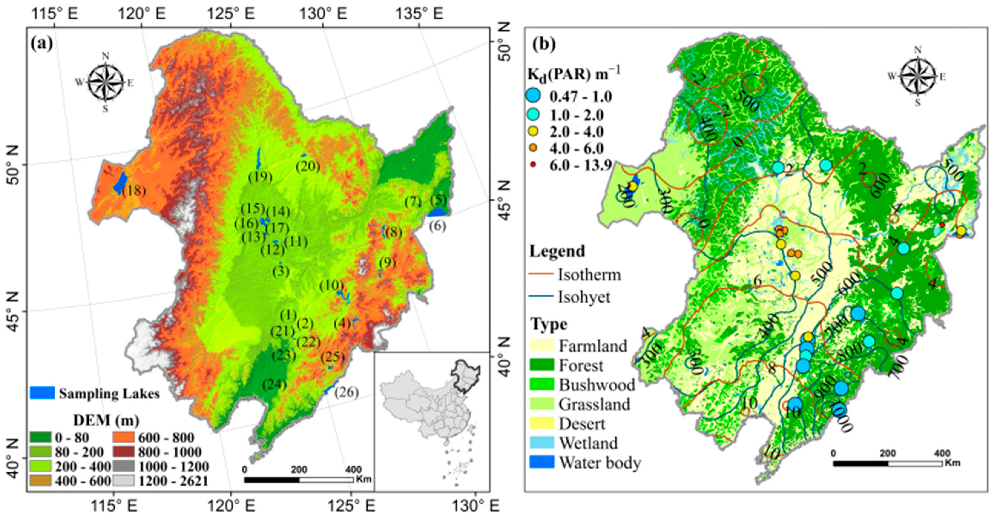
2.1. Study Area

Northeast China is an important base of agriculture, forestry, energy and heavy industry. The region which extends from 38°N to 54.0°N and 116°E to 136°E, includes all of the Heilongjiang, Jilin and Liaoning Provinces, and parts of Inner Mongolia Province. Its topography is characterized by mountains to the east, north and west that surround the Sanjiang, Songnen, and Liaohe Plains (Figure 1a). The region has a temperate continental monsoon climate which is controlled by the East Asian monsoons. This climate is characterized for its cool and short summers and for its cold and long winters with the lakes being frozen in winters. The annual average temperature ranges between −4 and 12 °C with a gradual increase from north to south. Precipitation is generally higher in the summer and autumn seasons and decreases from 1100 mm in the southeast to 250 mm in the west [42].
Forests are predominantly distributed in mountainous areas where the soil erosion is weak. Grasslands are mainly distributed in the Inner Mongolia plateau where the precipitation is generally less than 400 mm (Figure 1b). A large amount of lakes and reservoirs with various features are distributed in Northeast China. Reservoirs are mainly located in mountainous areas and are very deep with long-narrow shapes. Unlike reservoirs, most of the lakes are generally shallow and are located in plain areas, particularly in Western Songnen Plain. Due to the character of environmental factors like unevenly distributed precipitation, high evaporation and geomorphology of terminal-flow areas, many fresh and saline water bodies are distributed in the Songnen Plain [39].

2.2. In Situ Data Collection and Analysis

In total, 206 stations with measurement of PAR collected in six field experiments were used. The stations covered 26 lakes and reservoirs in Northeast China. Details about the distribution of the sample points are shown in Figure S1 (Supplementary Materials). There are only two lakes with areas less than 10 km2. The water approximately 0.5 m below the surface was collected in the acid-washed HDPE bottles for laboratory analysis. The location of each station was recorded with a UniStrong G3 GPS uint. Water transparency (Secchi disk depth, SDD) was measured with a 30 cm diameter black and white quadrant (Secchi) disk. PAR was measured by the Li-Cor 193SA underwater spherical quantum sensor on the sunny side of the boat to avoid any shadow effects. After posing the sensor at one depth in the water, PAR value was continuously recorded for 15 s and output an averaged value by the data logger. This value was regarded as the PAR value at this depth. The PAR measurements were taken at no less than five point’s depth for each station. Kd(PAR) was determined by applying the exponential regression model which utilizes Equation (1) [33], provided that the water column was homogeneous. The results were accepted only if the coefficient of determination (R2) was no less than 0.95 [7] and the number of depth points was no less than 4. In Equation (1), the PAR(Z) represents the PAR value at depth Z and PAR(0) represents the PAR value just beneath the surface of the water.
PAR ( Z ) = PAR ( 0 ) × exp [ K d ( PAR ) × Z ]

2.3. Water Quality Parameters

To determine the water quality, we calculated the concentrations of TSM and Chl-a, and the absorption of CDOM, phytoplankton and non-algal particles (NAP), as follows.
TSM concentration: For all samples, the concentration of TSM was determined gravimetrically. Whatman GF/F glass fiber filters (47 mm in diameter, 0.7 μm in average pore size) were initially combusted at 400 °C for 4 h to remove any organic matters on the filters. After cooling, they were weighed before proceeding to filtration. The volumes of water samples to be filtered were determined by their turbidity. The used filters were stored at 4 °C and re-weighed after drying for 4 h at 105 °C. The concentration of the TSM was calculated by dividing the difference of weight by the volume of the corresponding water sample.
Chl-a concentration: Chl-a was determined spectrophotometrically [43,44]. A certain volume (V) of water sample was filtered through GF/F cellulose acetate membrane filters with 47 mm in diameter and 0.47 μm in pore size. The filters were frozen at −20 °C and stored under dark conditions until further analysis. Pigments were extracted by soaking the mashed filters in 10 mL of 90% acetone solution for 24 h under dark conditions. The supernatant was collected after centrifugation (5000 r/min, 20 min) and its absorbance at 630, 647, 664 and 750 nm was measured by the Shimadzu UV-2600 PC spectrophotometer. Concentration of Chl-a was calculated by Equation (2) [45], where OD(630), OD(647), OD(664) and OD(750) represented the absorbance at 630, 647, 664 and 750 nm, respectively. The number 10 is the volume of the acetone solution. V is the volume of water sample in liter. L is the cuvette path length in cm. The cuvette with path length of 1 cm was used in this study.
Chl - a = { 11 . 85 × [ OD ( 664 ) OD ( 750 ) ] 1 . 54 × [ OD ( 647 ) OD ( 750 ) ] 0 . 08 × [ OD ( 630 ) OD ( 750 ) ] } × 10 / ( V × L )
CDOM absorption: The generally high concentration of particles in inland waters results in the difficulties in collecting enough filtrate for measurement by solely filtering water samples through 0.22 μm filters as the particles block the pore easily. Thus, water samples were initially filtered through 0.7 μm (pore size) Whatman GF/F glass fiber filters (pre-combusted at 400 °C for 4 h in a Muffle furnace) and then through 0.22 μm (pore size) nuclepore filters (Whatman) [2]. Then spectrophotometer (Shimadzu UV-2600) was used to measure the CDOM absorbance spectra (OD(λ)) between 200 and 800 nm at 1 nm intervals with the filtrate in 1 cm quartz cuvette and Milli-Q water as reference. The absorption spectrum (aCDOM(λ)) was calculated from the absorbance using Equation (3) [46], where L is the cuvette path length (0.01 m) and 2.303 is the conversion factor. Some fine particles may have remained in the filtrate so backscattering caused by them should be corrected with absorption of CDOM was assumed to be zero at λ0, where λ0 equals to 700 nm [2].
a CDOM ( λ ) = 2 . 303 L × [ OD ( λ ) OD ( λ 0 ) × ( λ / λ 0 ) ]
The absorption coefficient at 355 nm (aCDOM(355)) was selected to represent the CDOM concentration [47,48].
Absorption coefficients of phytoplankton (aph) and NAP (aNAP) were measured by the quantitative filter technique (QFT). A certain volume of each water sample was filtered through Whatman GF/F filter with a nominal pore size of 0.7 μm. Absorption of total particles (ap) on the filter was measured by spectrophotometer (Shimadzu UV-2600), and then aNAP was measured after the filter was bleached by sodium hypochlorite solution to remove the pigment. As for phytoplankton absorption, aph was calculated by subtracting aNAP from ap. The details can be found in [40,49]. Due to the artificial factors during the experiment, only ap of each sample point were measured for Baishan Reservoir (BSR number 4, Table 1).

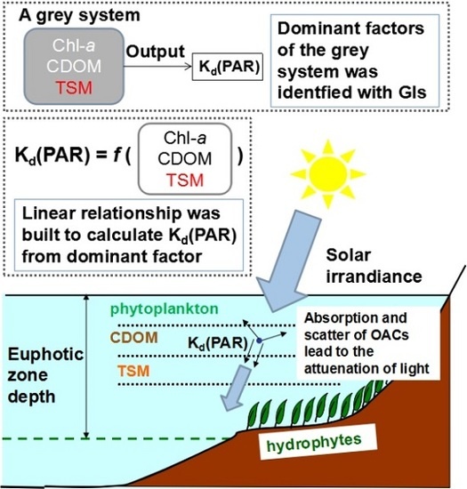
2.4. Grey Incidences (GIs) Analysis

The grey system theory is a method of processing and analyzing systems with incomplete information [50]. It has been used in remote sensing applications [51]. GIs provide a quantitative description of the system and dominant factor which influences the system’s development can be determined with GIs. Given a system contains m factors and one output, for k times of tests of the system, it generates a data sequence with k values of the output as Equation (4). This data sequence is defined as systematic behavior. The corresponding factors compose m data sequences that each contains k values (Equation (5)). This data sequences are defined as factor’s behavior.
X0 = {x0(k), k = 1, 2…n}
Xi = {xi(k), k = 1, 2…n} (i = 1, 2, 3…m)
In Equations (4) and (5), X0 and Xi represent the data sequences, x0(k) is the system output at kth test, and xi(k) is system factor value of ith factor at kth test. GIs describe the developmental trends of behaviors and factors in a system by analyzing the similarity of geometric patterns between systematic behavior and factor’s behavior data sequences [50]. By calculating and comparing GIs between X0 and Xi, the most influential factors could be identified.
In this research, Kd(PAR) of the sample points was regarded as the systematic behavior meanwhile corresponding Chl-a, TSM, and CDOM were regarded as factor’s behavior. Three types of GI were calculated. The first one (GI1) was proposed by Deng [52] and the details about calculation can be found in [53]. GI1 was the first model proposed in grey system theory. It measured the trend of system behaviors and factors by the distance between corresponding points of the data sequences. The second one (GI2) was the improved generalized absolute grey incidence model proposed by Cao and the details about its calculation can be found in [50]. GI2 is the modification of the GI proposed by Liu [53]. It measured the trend of system behaviors and factors by the area of the region that surrounded by the curves of the data sequences. Finally, the third one (GI3) was the absolute degree of grey incidence proposed by Mei [54]. According to GI3 model, data sequences X0 and Xi were converted to Y0 = {y0(k), k = 1, 2,…,n − 1} and Yi = {yi(k), k = 1, 2,…,n − 1}, respectively, using Equation (6). This conversion calculates the slopes of the adjacent data points in each data sequence.
y(k) = x(k + 1) − x(k) k = 1, 2, 3,…,n − 1
GI ( X 0 , X i ) = 1 n 1 i = 1 n 1 1 1 + | y 0 ( k ) y i ( k ) |
The GI of two data sequences (GI(X0,Xi)) was calculated from Equation (7). As shown above, the GI3 measured the trend of system behaviors and factors by the slope of the data sequences.
In order to eliminate influence of dimension, the data sequences were standardized to values ranging from 0 to 1 according to Equation (8) before calculating the three kinds of GIs.
x i ( k ) = x i ( k ) min ( X ) max ( X ) min ( X )

2.5. Linear Regression between Kd(PAR) and OACs

GIs provided the means to identify which of the OACs acts as the dominant factor in determining Kd(PAR), however it does not provide a relationship to quantitatively derive Kd(PAR) from the factor. Therefore, a linear regression analysis was performed to establish the quantitative relationship between Kd(PAR) and the concentration of the OACs. In some researches the regression analysis was also used to identify the dominant factor of Kd(PAR) [2,7] so it can also be used to validate the result of GIs analysis in this paper. In order to further evaluate the applicability of the predicting model, we first used the leave-one-out cross validation (LOO-CV) method and then accessed the model’s spatial transferability. For the LOO-CV analysis, n − 1 samples were used to calibrate Kd(PAR) and the sample left out was used to validate the model. Similarly, leave one lake out cross validation was used for the assessment of spatial transferability, sample points from n − 1 lakes were used to calibrate the Kd(PAR) and the sample points of the lake that was left out were used for validation. The prediction error sum of squares (PRESS) was used to derive the root-mean-square error of cross-validation (RMSECV) of the LOO-CV. Moreover, the relative error (RE), the mean relative error (MRE), and the root-mean-square error (RMSE) were used to assess the accuracy of the model. The details on how to calculate these indicators can be found in [12,44].

2.6. Relationship between Kd(PAR) and SDD

Water transparency is an easily measured indicator of water quality and is used to calculate the trophic state index [55]. SDD is correlated with Kd(PAR) as they are both influenced by the absorption and scatter characteristics of the OACs; in effect, both measurements represent the penetration of light in the water [56]. The difference between them is the varied contributions of the extent of spectral bands as SDD is related to the visible domain (410–665 nm) [57,58] and Kd(PAR) is 400–700 nm [5,33]. Kd(PAR) and SDD are inversely correlated since higher Kd(PAR) values indicate lower water clarity. The relationship of SDD and Kd(PAR) as defined by Holmes [8] is:
Kd(PAR) = f × SDD−1
where f has the value of 1.44 for turbid coastal waters [8]. However, other studies have reported different values of f, ranging from 1.7 to 2.3 [59,60]. In this paper, f was determined by linear regression with a fixed intercept at 0. With the relationship Kd(PAR) can be estimated from SDD.

3. Results and Discussion

3.1. Water Quality Characteristics

Due to the different geographical environments, the sampled area included a large diversity of inland waters with varying concentration of OACs (Table 1). The concentration of Chl-a (average: 15.16 ± 15.78 μg/L) varied from 1.20 (sample point number 10 of NEJR, number 19, Table 1) to 67.15 μg/L (sample point number 1 of LMSP, number 13, Table 1). BSR (number 4, Table 1) exhibited the largest variation of Chl-a ranging from 6.36 to 60.94 μg/L (average: 28.02 ± 20.35 μg/L) attributed to its long-narrow shape. Upstream regions contained high concentration of Chl-a. As the water depth becomes deep and flow velocity becomes slow from upstream to downstream regions, the suspended components sunken so concentration of Chl-a gradually decreased in the up layer of the water. The TSM concentration ranged from 0.83 (sample point number 3 of SHL, number 10, Table 1) to 184 mg/L (sample point number 4 of QNR, number 7, Table 1), with an average of 4.55 ± 28.25 mg/L. The highest concentration appeared in QNR (average: 174.5 ± 8.85 mg/L) and the lowest was in SHL (average: 1.48 ± 0.97 mg/L). XMP (number 3, Table 1) had the largest variation in the concentration of TSM (range: 10.75 to 64 mg/L, average: 26.01 ± 17.32 mg/L). This variation resulted from one particular sample point with very high TSM concentration (64 mg/L). It was collected in a site with high water turbulence as it located at the junction of a river and the lake. The absorption coefficient of CDOM at 355 nm was high both in XSTR (10.56 ± 0.25 m1, number 2, Table 1) and KLP (10.56 ± 0.44 m1, number 11, Table 1) due to their grayish yellow water color.
The SDD ranged from 0.1 to 4.32 m (Table 1). QNR (number 7, Table 1) had the lowest water clarity (0.11 ± 0.01 m), while HRR (number 25, Table 1) was the clearest (2.74 ± 0.34 m). The coefficient f fitted from all sample points was equal to 1.38 (R2 = 0.97) (Figure 2a). This result was closer to the one reported by Holmes [8] indicating that the equation proposed therein can be used to predict the Kd(PAR) from the SDD measurements.

3.2. Spatial Distribution of Kd(PAR)

The mean Kd(PAR) of each lake and their corresponding geographical distribution are shown in Figure 1b. In general, the reservoirs displayed low Kd(PAR) values. The reason might be due to the fact that they are located in mountainous areas, which are covered by forests that prevent soil erosion, hence, resulting in low concentrations of TSM. Lakes distributed in the Songnen Plain overall displayed high Kd(PAR) values. The soil erosion around these lakes was strong, the lakes were shallow, and the re-suspension caused by strong winds in the area also contributed to high turbidity [39]. These findings were in agreement with the research conducted by Olmanson [61], which revealed that lakes of Minnesota that were located in forest regions were clearer than those located in plain regions.

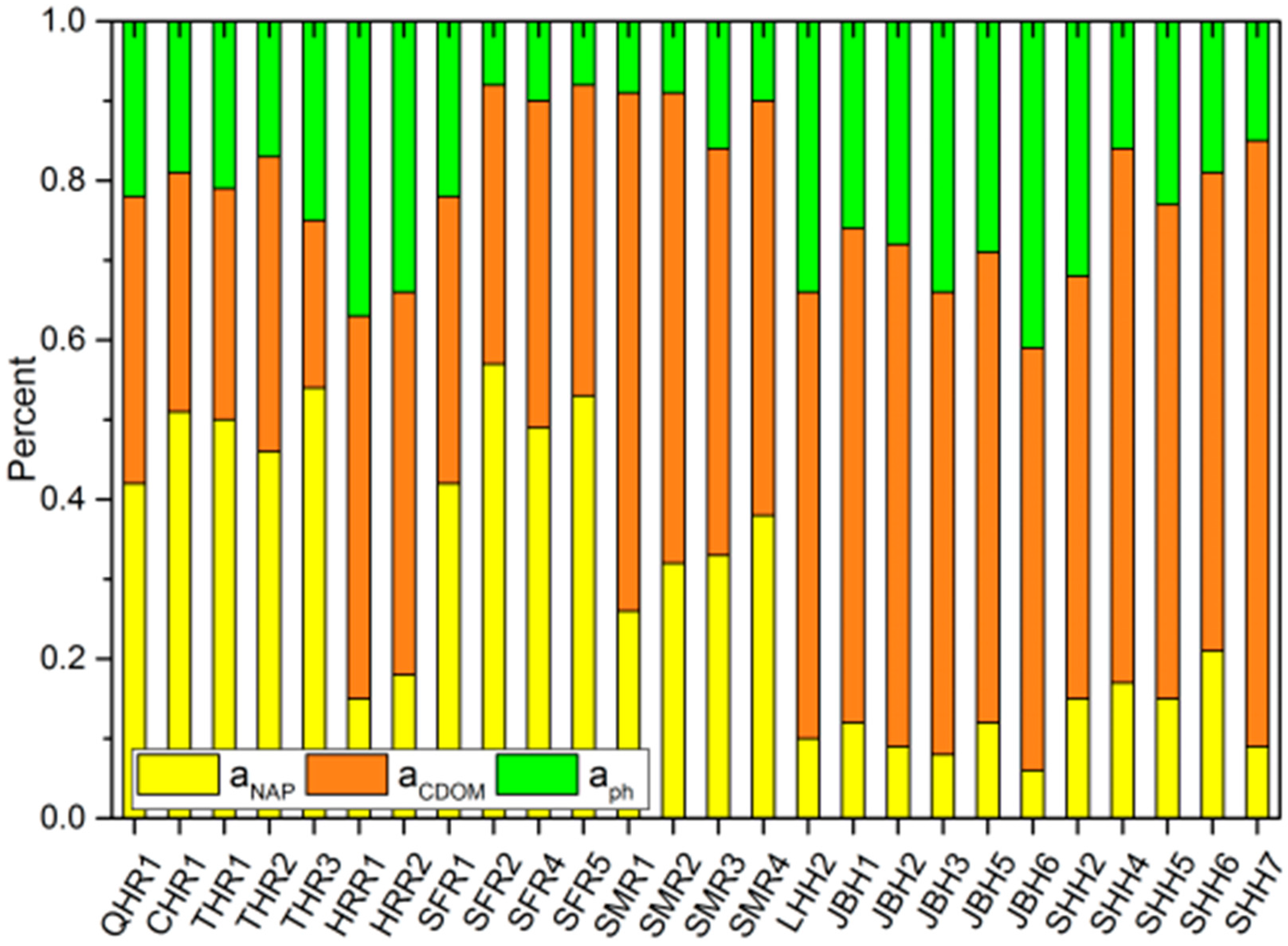
3.3. Grey Incidences between Kd(PAR) and OACs

According to previous studies [48], absorption coefficient at 355 nm of CDOM (aCDOM(355)) was regarded as a representative measure of the concentration of CDOM. GIs were calculated with TSM, Chl-a and aCDOM(355) as the factor’s behavior data sequences while Kd(PAR) as the systematic behavior data sequence. The factor with higher GIs score indicates a relative bigger influence on Kd(PAR). The GIs of all the sample points were calculated and the results (Table 2) showed that the highest GIs were obtained by comparing between TSM and Kd(PAR). These results indicated that TSM had a higher contribution to Kd(PAR) than Chl-a and CDOM, which is consistent with previous studies in Lake Taihu in China [7,12] and UK marine waters [10]. Furthermore, in order to assess the difference of the relationships across various waters, lakes with more than 10 sampling points were also selected to calculate GIs individually. The results (Table 2) indicated that the dominant factors of Kd(PAR) varied according to lakes. For example, Kd(PAR) of BSR may largely influenced by TSM and Chl-a as the GIs of two materials did not vary significantly.

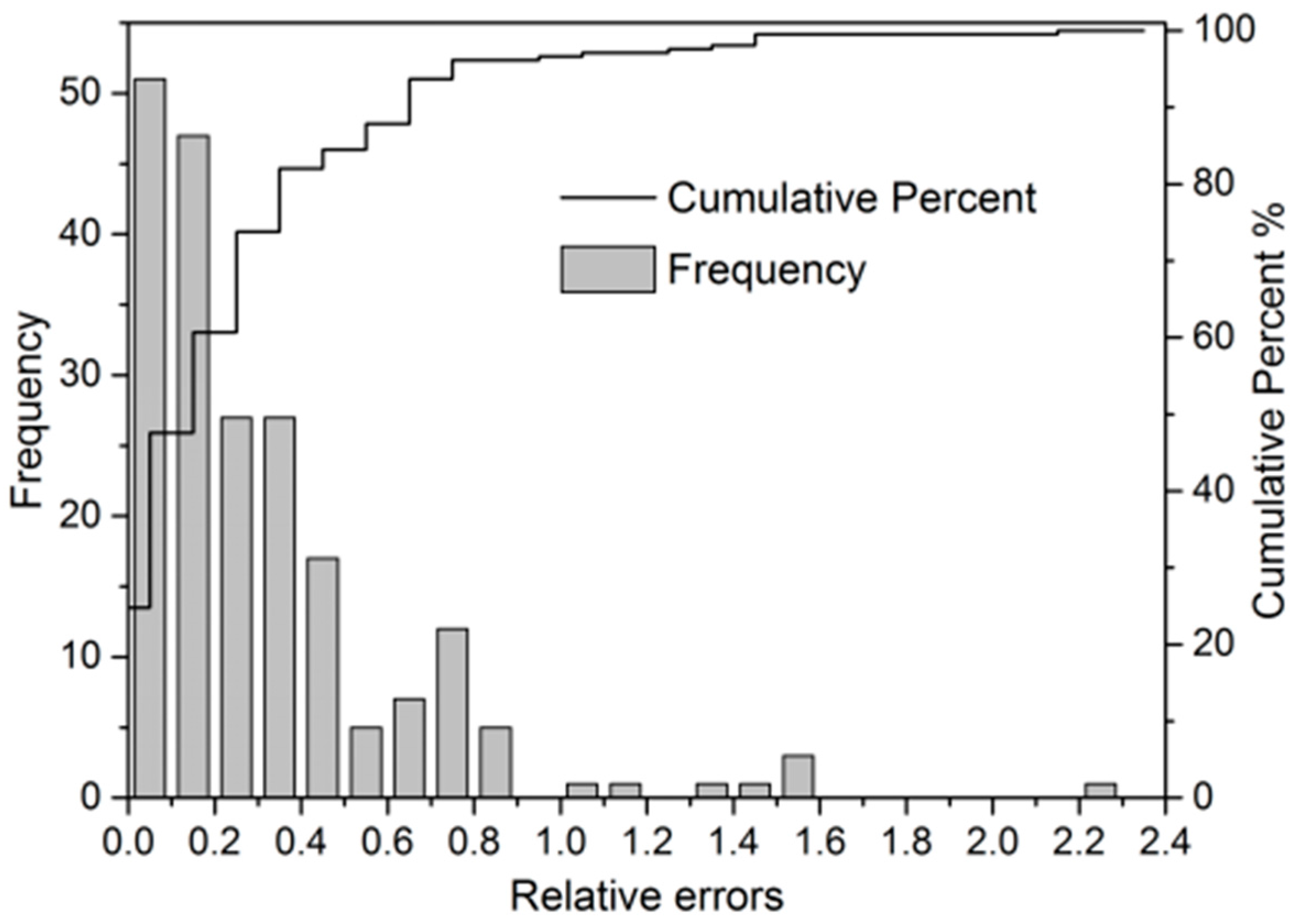
3.4. Kd(PAR) Model Calibration and Validation

In this study, TSM was revealed to be the major impact factor for the determination of Kd(PAR). The linear regression analysis provided the means to predict Kd(PAR) by utilizing the OACs data. The results indicated that Kd(PAR) was strongly correlated to TSM, while there was no obvious relationship between Kd(PAR) and Chl-a or CDOM (Figure 2). The mean value of Kd(PAR) and OACs of each lake were determined by averaging all the sample points collected from the corresponding lakes. The coefficient of determination (R2) was improved when averaged value of each lake, rather than all the single point values, was fitted in the linear model. This is because experimental error may exist in a single sample point, which leads to the dispersion of the data. The average of the data can eliminate the error to some extent and result in a stable performance. The slope of the linear model between Kd(PAR) and TSM in the current study was slightly higher than results in [7] (slope = 0.0626, intercept = 1.6068) and [12] (slope = 0.0563, intercept = 1.52). Considered that our research covered a larger number of lakes than those earlier studies, such a difference was acceptable. The results of linear regression also indicated that the dominant factor of Kd(PAR) for lakes of Northeastern China is TSM as the GIs indicated. This result provides a guidance in band selection to derive Kd(PAR) from remote sensing image that the bands well correlate to TSM may perform well in deriving Kd(PAR) [12]. The model estimating Kd(PAR) from TSM may be applied in mapping Kd(PAR) indirectly from remote sensing image. The dominant factor of Kd(PAR) for lakes in Northeastern China was same to Lake Taihu, a large shallow lake in Eastern China [2,7,12]. However, the coefficients of the linear relationship indicated there was difference in optical properties between Lake Taihu and lakes in Northeastern China.
A multivariate linear regression analysis was also performed with Kd(PAR) as dependent variable and TSM, Chl-a and aCDOM(355) as independent variables. A slight better fit was obtained as the R2 was 0.916 for all sample point values and 0.960 for lake specified mean values. The result was similar to those of Zhang [2] and Devlin [11], demonstrating that slight improved models were achieved when fit Kd(PAR) with all three explanatory variables rather than solely TSM for waters that Kd(PAR) was mainly influenced by TSM.
The simple linear model may be suitable for predicting Kd(PAR) from TSM as it produced low error rates (RMSE: 0.689 for lake averaged values, and 0.709 for single point values). The RMSECV of the LOO-CV analysis was 0.709 and the MAPE was 0.315. The RE which was used for validation ranged from 0.0016 to 2.2 (Figure 3). The relative error of 61% of the samples was below 0.3 and of 74% of the samples was below 0.4. Altogether our results indicated that the TSM performed well in estimating Kd(PAR). However, care should be taken when applying this model to some cases as TSM might not always represent the major determining factor of Kd(PAR). This could be the case of eight sample points in our study which displayed RE values larger than 1.0 in LOO-CV.
To investigate this further, 32 points, whose RE of LOO-CV was greater than 0.6, were selected to analyze the relationship between Kd(PAR) and OACs. For the 32 sample points, the averaged Kd(PAR) was 0.727 ± 0.150 m−1 and the large RE value was mainly caused by the overestimation of the model (see Figure S2). The linear regression analysis (see Figure S3) indicated that Kd(PAR) had a better correlation with the concentration of TSM (R2 = 0.60) than with Chl-a and CDOM (R2 < 0.1). However, when compared to the model built by all sample points, the slope and intercept decreased to 0.06 and 0.522, respectively. This explained why the model built with all sample points lead to overestimation of Kd(PAR) for the 32 sample points. However, the GIs revealed that the correlation between the OACs (TSM, Chl-a, CDOM) and Kd(PAR) did not vary significantly (GI1: 0.70, 0.65, 0.68), (GI2: 0.55, 0.67, 0.72) and (GI3: 0.91, 0.80, 0.80),which indicated that the dominant factors of Kd(PAR) may not solely TSM for this 32 sample points. The R2 of multivariate linear regression analysis was 0.64, which implied an improved fit with TSM, Chl-a and CDOM.
The integration of the absorption coefficient curves between 400–700 nm were used to calculate the relative contribution of phytoplankton, NAP and CDOM to the total absorption of the samples (Figure 4). Due to the absorption spectra of phytoplankton and NAP in the BSR were not measured, therefore, six data points from BSR were not analyzed further. Nonetheless, the absorption spectra of the total particulate matter showed an obvious peak at 675 nm (see Figure S4), which indicated that the contribution of the phytoplankton to the total absorption is strong. The total absorption of HRR was dominated by CDOM and phytoplankton which might cause the large error observed by solely estimating Kd(PAR) from TSM. Though NAP contributed more than phytoplankton and CDOM to the total absorption of QHR1, CHR1, THR and SFR, high RE were observed when predicting Kd(PAR) solely from the TSM. This might be attributed to the extremely clear water which makes the model unsuitable for this type of environment; therefore, a separate analysis should be done for this lake. For JBL and SHL, the CDOM was the main contributor to the total absorption, thus, the Kd(PAR) may have a good correlation with it, as discussed in Section 3.5.

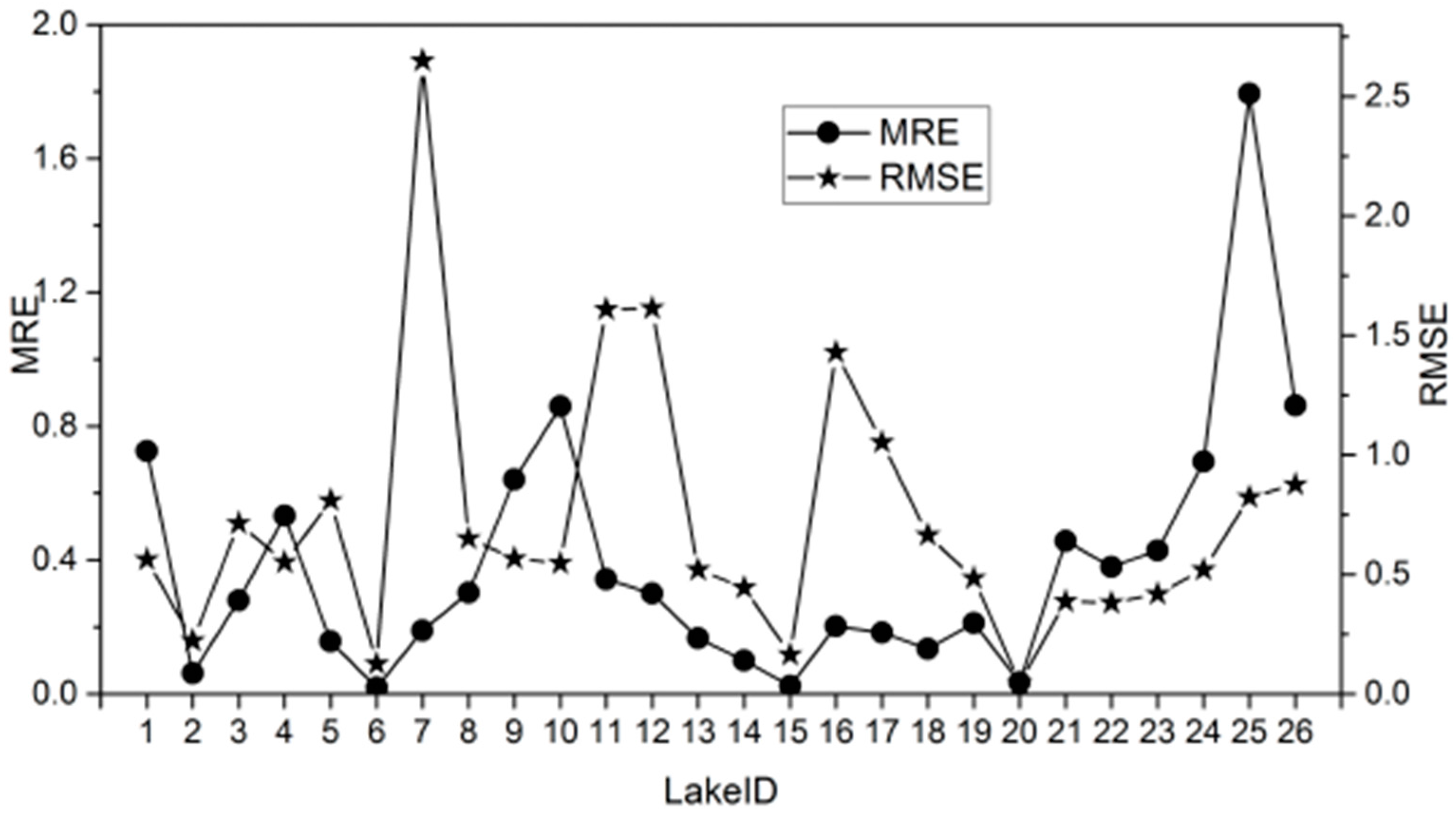
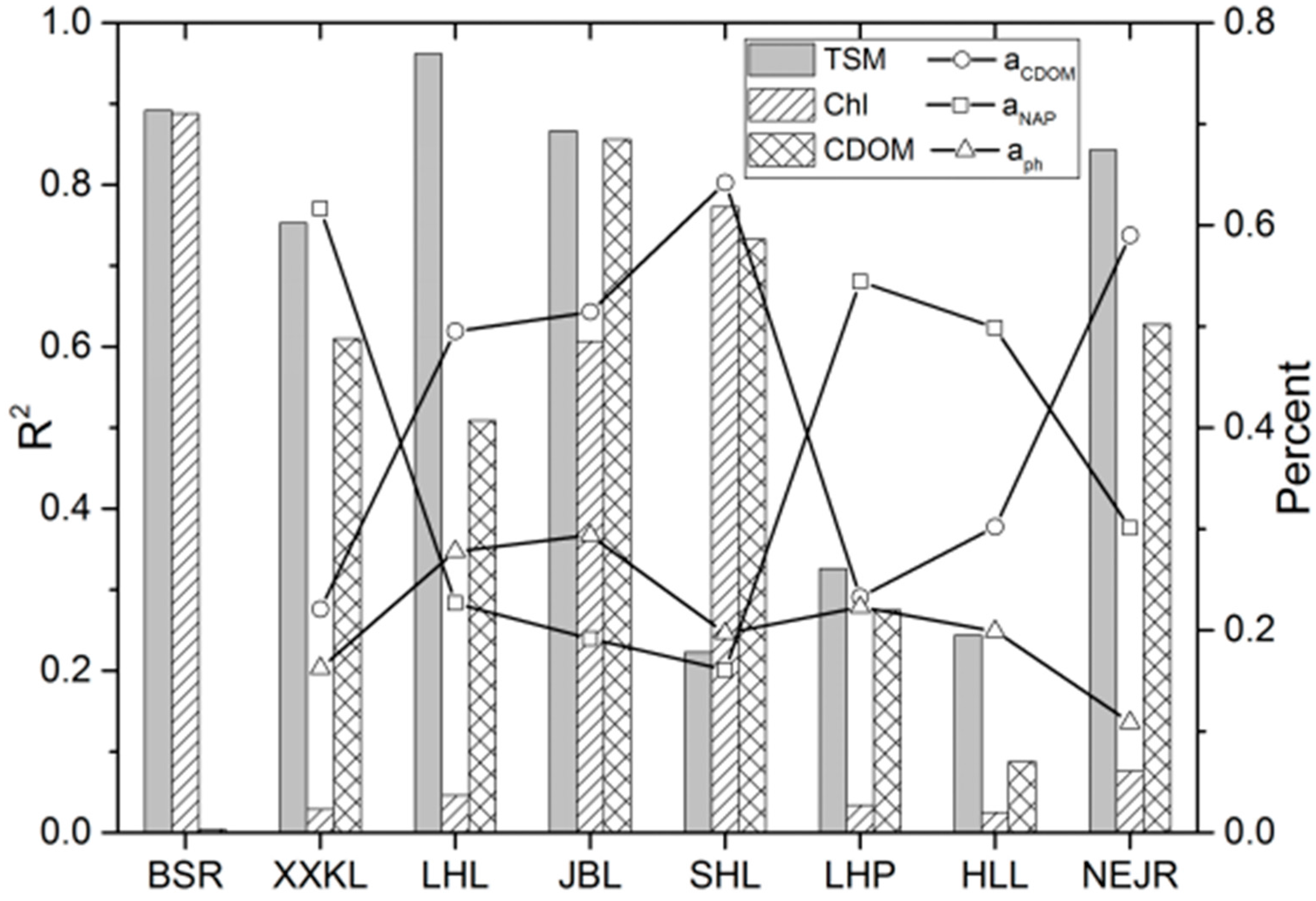
3.5. Spatial Transferability

The MRE and RMSE of each lake were calculated in the spatial transferability assessment (Figure 5). QNR (LakeID: 7), KLP (LakeID: 11), NYR (LakeID: 12), and XHLP (LakeID: 16) all had high RMSE values but relatively low MRE values due to their high Kd(PAR). Unlike the RMSE values, which were low for HHR (LakeID: 25), SFR (LakeID: 26), SHL (LakeID: 10) SMR (LakeID: 1), THR (LakeID: 24), JBL (LakeID: 9) and BSR (LakeID: 4) (Figure 5), the MRE (MRE: 1.794, 0.862, 0.860, 0.726, 0.694, 0.641 and 0.532, respectively) indicated that there were large errors in predicting Kd(PAR) in this lakes. These lakes commonly had low levels of TSM, so the relative contributions of Chl-a and CDOM could not be eliminated from the analysis as they may also have large influence on Kd(PAR). Otherwise, it may cause the high MRE values in predicting Kd(PAR) solely with TSM.
In order to identify the differential contribution of OACs to the estimation of Kd(PAR) across different lakes, a separate analysis was undertaken for lakes with more than 10 sample points. Although only six sample points were obtained from SHL, it was still selected because it was the second clearest lake in this study, and it had RE greater than 0.4 in the LOO-CV analysis. The GIs for the lakes were calculated respectively and linear regression between OACs and Kd(PAR) was performed. The lake specified averaged absorption spectra were used to calculate the relative contribution of phytoplankton, NAP and CDOM to the total absorption of each lake. The R2 of linear regression and the relative contribution were shown in Figure 6.
GIs of the lakes are shown in Table 2. For SHL, the GIs between the OACs (TSM, Chl-a, CDOM) and the Kd(PAR) are (GI1: 0.62, 0.81, 0.67), (GI2: 0.77, 0.90, 0.80) and (GI3: 0.77, 0.89, 0.83). The GIs of SHL showed that Chl-a and CDOM displayed a higher correlation than TSM with the Kd(PAR), and this was consistent with the results obtained by linear regression analysis. The contribution of CDOM and phytoplankton to the total absorption was larger than NAP and this could explain why Kd(PAR) was mainly influenced by Chl-a and CDOM. The R2 of the correlation analysis revealed that the Kd(PAR) of BSR was highly related to both TSM and Chl-a, and that there was only a minor variation in the GIs of TSM and Chl-a. The Kd(PAR) of NEJR was greatly correlated to both TSM and CDOM, and CDOM and NAP contributed more to the total absorption. This was similar to the analyzing results of XXKH. Overall, the count of dominant factors for determining Kd(PAR) were two rather one in the cases of the lakes/reservoirs described above. This results is consistent with the findings in Danjiangkou Reservoir (averaged Kd(PAR) was 0.726 m−1) in Hubei Province, China [32]. That study revealed that TSM and Chl-a dominated Kd(PAR) during the wet season while Chl-a and CDOM were the major determinants of Kd(PAR) in the dry season in the reservoir.
The TSM and CDOM concentrations were well correlated to Kd(PAR) for JBL. Similarly, Chl-a also had a modest correlation with Kd(PAR). In contrast to JBL which displayed similar contributions of each constituent to the total absorption, the Kd(PAR) of LHL was mainly correlated to the TSM. The reason may be that the TSM was more varied in LHL (range: 2.83–22.6 mg/L, StDev: 6.33) than in JBL (range: 2.14–10.2 mg/L, StDev: 2.3), while the Chl-a was more varied in JBL (range: 9.94–61.67 μg/L, StDev: 14.61) than in LHL (range: 6.81–43.11 μg/L, StDev: 10.43). Though NAP contributed the most to the total absorption in LHP and HLH, Kd(PAR) had a weak correlation with the TSM. Taking into account that these two lakes are vast in shape and relative shallow in depth (5.92 m for HLH and 2.7 m for LHP) [37], it is possible that the OACs are uniformly distributed in the water causing a little variation in the calculation of Kd(PAR) across different sample points. This might have produced low standard deviations in the values of the dependent and the independent variables, in effect, lowering the significance of the linear correlation. In addition, the measurement of PAR was easily influenced by waves in these lakes which could induce large errors to the calculation of Kd(PAR). These errors could contribute to the reduction of the correlation between the Kd(PAR) and the OACs in HLH and LHP. There was an inconformity that a factor showed a high contribution to the total absorption might not be best correlated to the Kd(PAR). This inconformity was also observed by Shi [29] in Bosten Lake in Xinjiang Province, China. In his study, both CDOM and phytoplankton contributed more than NAP to the total absorption, however, the Kd(PAR) was best correlated to the TSM concentration.

4. Conclusions

Based on the data collected in Northeast China, the relationships between Kd(PAR) and OACs were studied. The optical properties of water bodies were diverse and complex. Kd(PAR) was significantly correlated to the water transparency (SDD) and the coefficient was in agreement with previous studies [8]. According to GIs and linear regression analysis of the data of all the sampled points, it was found that TSM was the most dominant component of the OACs in regulating Kd(PAR). As a systemic analysis method, GIs were effective in identifying the dominant factors of Kd(PAR). The TSM accounted for the most variation of the Kd(PAR) as the R2 of the linear model only increased 0.01 when TSM, Chl-a, and CDOM were the explanatory variables rather than solely TSM was the explanatory variable. The investigation of the simple linear model demonstrated that it was an effective tool to predict Kd(PAR) from TSM data as it produced small RE in a LOO-CV analysis. However, the dominant regulating factors of Kd(PAR) varied among some of the sample points and lakes, especially for some clear waters, in which the dominant factors may be a combination of two or three kinds of OACs. This variation can be attributed to their distinct geographical environments. Lakes that are open in shape and shallow in depth and distributed in plain areas, where soil erosion is relatively strong, show high Kd(PAR) values. Therefore, the major determining factor of Kd(PAR) in these types of lakes is the concentration of TSM. However, for very clear water bodies, for example in deep and narrow reservoirs, which are distributed in mountainous areas where soil erosion is weak, the concentration of the TSM is low. In such cases, the contribution of the concentrations of Chl-a and/or CDOM to the estimation of Kd(PAR) is also significant. There was a discrepancy in the results derived from correlation analysis and from absorption spectra analysis. The material which contributed the most to the total absorption may not be well correlated to the Kd(PAR) due to the scattering of phytoplankton and TSM also affect Kd(PAR) [29]. In general, reservoirs in the east part of Northeast China had low Kd(PAR) values, while lakes located in plain areas showed high Kd(PAR) values. These differences in the Kd(PAR) could reflect variations in the composition of TSM in these distinct geographical locations.

Supplementary Materials

The following are available online at www.mdpi.com/2072-4292/8/11/964/s1, Figure S1: Distribution of sample points of each lakes or reservoirs. The color represents the average Kd(PAR), the number and abbreviation were listed in Table 1; Figure S2: The estimated Kd(PAR) by TSM and in situ Kd(PAR) for sample points that had relative error (RE) greater than 0.6 in LOO-CV. Eight sample points had RE greater than 1 and they were HRR1 (RE: 2.20), JBH1 (RE: 1.59), JBH3(RE: 1.54), SHH7(RE: 1.50), SFR5(RE: 1.49), HRR2(RE: 1.36), SHH5(RE: 1.15) and QHR1(RE: 1.06); Figure S3: Linear regression analysis between OACs and Kd(PAR) for sample points that had relative error (RE) greater than 0.6 in LOO-CV. (a) total suspended matter (TSM); (b) chlorophyll-a(Chl-a); (c) absorption coefficient of chromophroic dissolved organic matter (CDOM) at 355 nm (aCDOM(355)); Figure S4: Absorption coefficient of total particulate materials of BSR. Only the absorption coefficients of total particulate materials were measured during the experiment but the phytoplankton and non-algal particles were not measured. The obvious absorption peak at 675 nm indicated the pigment absorption was dominant in the total particulate absorption.

Acknowledgments

The research was jointly supported by the “One Hundred Talents” program from Chinese Academy of Sciences granted to Kaishan Song, the National Natural Science Foundation of China (No. 41471290, No. 41501387) and the Foundation of China’s High Resolution Earth Observation (No. 41-Y20A31-9003-15/17). The authors thank Jia Du, Ming Wang, and Junbin Hou for their persistent assistance with field sampling and in situ measurements. The authors also thank the editors and three anonymous reviewers for their valuable and instructive comments that have strengthened the manuscript greatly.

Author Contributions

Kaishan Song conceived the framework and designed the fieldwork; Zhidan Wen, Ying Zhao, Yingxin Shang, Chong Fang, Jia Du, and Jianhang Ma performed the fieldwork and experiments; Jianhang Ma analyzed the data and wrote the paper; and Jianhang Ma and Kaishan Song revised the paper.

Conflicts of Interest

The authors declare no conflict of interest.

References

  1. Lund-Hansen, L.C. Diffuse attenuation coefficients Kd(PAR) at the estuarine North Sea-Baltic Sea transition: Time-series, partitioning, absorption, and scattering. Estuar. Coast. Shelf Sci. 2004, 61, 251–259. [Google Scholar] [CrossRef]
  2. Zhang, Y.L.; Zhang, B.; Ma, R.H.; Feng, S.; Le, C.F. Optically active substances and their contributions to the underwater light climate in Lake Taihu, a large shallow lake in China. Fundam. Appl. Limnol. Arch. Hydrobiol. 2007, 170, 11–19. [Google Scholar] [CrossRef]
  3. Behrenfeld, M.J.; Falkowski, P.G. A consumer’s guide to phytoplankton primary productivity models. Limnol. Oceanogr. 1997, 42, 1479–1491. [Google Scholar] [CrossRef]
  4. Behrenfeld, M.J.; Falkowski, P.G. Photosynthetic rates derived from satellite-based chlorophyll concentration. Limnol. Oceanogr. 1997, 42, 1–20. [Google Scholar] [CrossRef]
  5. Kirk, J.T.O. Light and Photosynthesis in Aquatic Ecosystems; Cambridge University Press: New York, NY, USA, 1994. [Google Scholar]
  6. Chang, G.C.; Dickey, T.D. Coastal ocean optical influences on solar transmission and radiant heating rate. J. Geophys. Res. Oceans 2004, 109. [Google Scholar] [CrossRef]
  7. Zhang, Y.L.; Qin, B.Q.; Hu, W.P.; Wang, S.M.; Chen, Y.W.; Chen, W.M. Temporal-spatial variations of euphotic depth of typical lake regions in Lake Taihu and its ecological environmental significance. Sci. China Ser. D 2006, 49, 431–442. [Google Scholar] [CrossRef]
  8. Holmes, R.W. The Secchi disk in turbid coastal zones. Limnol. Oceanogr. 1970, 15, 688–694. [Google Scholar] [CrossRef]
  9. Shang, S.L.; Lee, Z.P.; Wei, G.M. Characterization of MODIS-derived euphotic zone depth: Results for the China Sea. Remote Sens. Environ. 2011, 115, 180–186. [Google Scholar] [CrossRef]
  10. Devlin, M.J.; Barry, J.; Mills, D.K.; Gowen, R.J.; Foden, J.; Sivyer, D.; Tett, P. Relationships between suspended particulate material, light attenuation and Secchi depth in UK marine waters. Estuar. Coast. Shelf Sci. 2008, 79, 429–439. [Google Scholar] [CrossRef]
  11. Devlin, M.J.; Barry, J.; Mills, D.K.; Gowen, R.J.; Foden, J.; Sivyer, D.; Greenwood, N.; Pearce, D.; Tett, P. Estimating the diffuse attenuation coefficient from optically active constituents in UK marine waters. Estuar. Coast. Shelf Sci. 2009, 82, 73–83. [Google Scholar] [CrossRef]
  12. Shi, K.; Zhang, Y.L.; Liu, X.H.; Wang, M.Z.; Qin, B.Q. Remote sensing of diffuse attenuation coefficient of photosynthetically active radiation in Lake Taihu using MERIS data. Remote Sens. Environ. 2014, 140, 365–377. [Google Scholar] [CrossRef]
  13. Zhang, Y.B.; Zhang, Y.L.; Zha, Y.; Shi, K.; Zhou, Y.Q.; Li, Y.L. Estimation of diffuse attenuation coefficient of photosynthetically active radiation in Xin’anjiang Reservoir based on Landsat 8 data. Chin. J. Environ. Sci. 2015, 36, 4420–4429, (In Chinese with English Abstract). [Google Scholar]
  14. Mueller, J.L. SeaWiFS algorithm for the diffuse attenuation coefficient, Kd(490), using water-leaving radiances at 490 and 555 nm. SeaWiFS Postlaunch calibration and validation analyses, part. Med. Today 2000, 5, 16–29. [Google Scholar]
  15. Chen, J.; Cui, T.W.; Tang, J.W.; Song, Q.J. Remote sensing of diffuse attenuation coefficient using MODIS imagery of turbid coastal waters: A case study in Bohai Sea. Remote Sens. Environ. 2014, 140, 78–93. [Google Scholar] [CrossRef]
  16. Majozi, N.P.; Salama, M.S.; Bernard, S.; Harper, D.M.; Habte, M.G. Remote sensing of euphotic depth in shallow tropical inland waters of Lake Naivasha using MERIS data. Remote Sens. Environ. 2014, 148, 178–189. [Google Scholar] [CrossRef]
  17. Ramon, D.; Jolivet, D.; Tan, J.; Frouin, R. Estimating photosynthetically available radiation at the ocean surface for primary production (3P Project): Modeling, evaluation, and application to global MERIS imagery. Proc. SPIE 2016. [Google Scholar] [CrossRef]
  18. Frouin, R.; McPherson, J. Estimating photosynthetically available radiation at the ocean surface from GOCI data. Ocean Sci. J. 2012, 47, 313–321. [Google Scholar] [CrossRef]
  19. Doron, M.; Babin, M.; Mangin, A.; Hembise, O. Estimation of light penetration, and horizontal and vertical visibility in oceanic and coastal waters from surface reflectance. J. Geophys. Res. Oceans 2007, 112. [Google Scholar] [CrossRef]
  20. Lee, Z.P.; Weidemann, A.; Kindle, J.; Arnone, R.; Carder, K.L.; Davis, C. Euphotic zone depth: Its derivation and implication to ocean color remote sensing. J. Geophys. Res. Oceans 2007, 112. [Google Scholar] [CrossRef]
  21. Son, S.H.; Wang, M.H. Diffuse attenuation coefficient of the photosynthetically available radiation Kd (PAR) for global open ocean and coastal waters. Remote Sens. Environ. 2015, 159, 250–258. [Google Scholar] [CrossRef]
  22. Alikas, K.; Kratzer, S.; Reinart, A.; Kauer, T.; Paavel, B. Robust remote sensing algorithms to derive the diffuse attenuation coefficient for lakes and coastal waters. Limnol. Oceanogr. Methods 2015, 13, 402–415. [Google Scholar] [CrossRef]
  23. Austin, R.W.; Petzold, T.J. The Determination of the Diffuse Attenuation Coefficient of Sea Water Using the Coastal Zone Color Scanner; Springer: New York, NY, USA, 1981. [Google Scholar]
  24. Mueller, J.L.; Trees, C.C. Revised SeaWiFS prelaunch algorithm for diffuse attenuation coefficient K (490). Case Stud. SeaWiFS Calibration Valid. 1997, 41, 18–21. [Google Scholar]
  25. Zhang, T.L.; Fell, F. An empirical algorithm for determining the diffuse attenuation coefficient Kd in clear and turbid waters from spectral remote sensing reflectance. Limnol. Oceanogr. Methods 2007, 5, 457–462. [Google Scholar] [CrossRef]
  26. Zhang, Y.L.; Liu, X.H.; Yin, Y.; Wang, M.Z.; Qin, B.Q. A simple optical model to estimate diffuse attenuation coefficient of photosynthetically active radiation in an extremely turbid lake from surface reflectance. Opt. Express 2012, 20, 20482–20493. [Google Scholar] [CrossRef] [PubMed]
  27. Phlips, E.J.; Aldridge, F.J.; Schelske, C.L.; Crisman, T.L. Relationships between light availability, chlorophyll a, and tripton in a large, shallow subtropical lake. Limnol. Oceanogr. 1995, 40, 416–421. [Google Scholar] [CrossRef]
  28. Morel, A.; Huot, Y.; Gentili, B.; Werdell, P.J.; Hooker, S.B.; Franz, B.A. Examining the consistency of products derived from various ocean color sensors in open ocean (Case 1) waters in the perspective of a multi-sensor approach. Remote Sens. Environ. 2007, 111, 69–88. [Google Scholar] [CrossRef]
  29. Shi, Z.Q.; Zhang, Y.L.; Yin, Y.; Liu, X.H. Characterization of the underwater light field and the affecting factors in Bosten Lake in summer. Acta Sci. Circumst. 2012, 32, 2969–2977, (In Chinese with English Abstract). [Google Scholar]
  30. Kratzer, S.; Hakansson, B.; Sahlin, C. Assessing Secchi and photic zone depth in the Baltic Sea from satellite data. AMBIO J. Hum. Environ. 2003, 32, 577–585. [Google Scholar] [CrossRef]
  31. Li, Y.L.; Zhang, Y.L.; Liu, M.L. Calculation and retrieval of euphotic depth of Lake Taihu by remote sensing. J. Lake Sci. 2009, 21, 165–172, (In Chinese with English Abstract). [Google Scholar]
  32. Qu, M.Y.; Cai, Q.H.; Shen, H.L.; Li, B. Variation and influencing factors of euphotic depth in Danjiangkou reservoir in different hydrological periods. Resour. Environ. Yangtze Basin 2014, 23, 53–59, (In Chinese with English Abstract). [Google Scholar]
  33. Pierson, D.C.; Kratzer, S.; Strömbeck, N.; Håkansson, B. Relationship between the attenuation of downwelling irradiance at 490 nm with the attenuation of PAR (400 nm–700 nm) in the Baltic Sea. Remote Sens. Environ. 2008, 112, 668–680. [Google Scholar] [CrossRef]
  34. Tan, J.; Cherkauer, K.A.; Chaubey, I. Using hyperspectral data to quantify water-quality parameters in the Wabash River and its tributaries, Indiana. Int. J. Remote Sens. 2015, 36, 5466–5484. [Google Scholar] [CrossRef]
  35. Tan, J.; Cherkauer, K.A.; Chaubey, I. Developing a comprehensive spectral-biogeochemical database of midwestern rivers for water quality retrieval using remote sensing data: A case study of the Wabash River and its tributary, Indiana. Remote Sens. 2016, 8, 517. [Google Scholar] [CrossRef]
  36. Li, N.; Liu, J.P.; Wang, Z.M. Dynamics and driving force of lake changes in northeast China during 2000–2010. J. Lake Sci. 2014, 26, 545–551, (In Chinese with English Abstract). [Google Scholar]
  37. Wang, S.M.; Dou, H.S. (Eds.) Chinese Lake Catalogue; Science Press: Beijing, China, 1998. (In Chinese)
  38. Duan, H.T.; Ma, R.H.; Zhang, Y.L.; Zhang, B. Remote-sensing assessment of regional inland lake water clarity in northeast China. Limnology 2009, 10, 135–141. [Google Scholar] [CrossRef]
  39. Song, K.S.; Zang, S.Y.; Zhao, Y.; Li, L.; Du, J.; Zhang, N.N.; Wang, X.D.; Shao, T.T.; Guan, Y.; Liu, L. Spatiotemporal characterization of dissolved carbon for inland waters in semi-humid/semi-arid region, China. Hydrol. Earth Syst. Sci. 2013, 17, 4269–4281. [Google Scholar] [CrossRef]
  40. Wen, Z.D.; Song, K.S.; Zhao, Y.; Du, J.; Ma, J.H. Influence of environmental factors on spectral characteristic of chromophoric dissolved organic matter (CDOM) in Inner Mongolia Plateau, China. Hydrol. Earth Syst. Sci. Discuss. 2015, 12, 5895–5929. [Google Scholar] [CrossRef]
  41. Zhao, Y.; Song, K.; Wen, Z.D.; Li, L.; Zang, S.Y.; Shao, T.T.; Li, S.J.; Du, J. Seasonal characterization of CDOM for lakes in semiarid regions of Northeast China using excitation–emission matrix fluorescence and parallel factor analysis (EEM–PARAFAC). Biogeosciences 2016, 13, 1635–1645. [Google Scholar] [CrossRef]
  42. Mao, D.H.; Wang, Z.M.; Wu, C.; Song, K.S.; Ren, C.Y. Examining forest net primary productivity dynamics and driving forces in northeastern China during 1982–2010. Chin. Geogr. Sci. 2014, 24, 631–646. [Google Scholar] [CrossRef]
  43. Song, K.S.; Wang, Z.M.; Blackwell, J.; Zhang, B.; Li, F.; Zhang, Y.Z.; Jiang, G.J. Water quality monitoring using Landsat Themate Mapper data with empirical algorithms in Chagan Lake, China. J. Appl. Remote Sens. 2011, 5, 053506. [Google Scholar] [CrossRef]
  44. Song, K.S.; Li, L.; Tedesco, L.P.; Li, S.; Duan, H.T.; Liu, D.W.; Hall, B.E.; Du, J.; Li, Z.C.; Shi, K.; et al. Remote estimation of chlorophyll—A in turbid inland waters: Three-band model versus GA-PLS model. Remote Sens. Environ. 2013, 136, 342–357. [Google Scholar] [CrossRef]
  45. Jeffrey, S.W.; Humphrey, G.F. New spectrophotometric equations for determining chlorophylls a, b, c1 and c2 in higher plants, algae and natural phytoplankton. Biochem. Physiol. Pflanz. 1975, 167, 191–194. [Google Scholar]
  46. Bricaud, A.; Morel, A.; Prieur, L. Absorption by dissolved organic matter of the sea (yellow substance) in the UV and visible domains. Limnol. Oceanogr. 1981, 26, 43–53. [Google Scholar] [CrossRef]
  47. Miller, R.L.; Belz, M.; Del Castillo, C.; Trzaska, R. Determining CDOM absorption spectra in diverse coastal environments using a multiple pathlength, liquid core waveguide system. Cont. Shelf Res. 2002, 22, 1301–1310. [Google Scholar] [CrossRef]
  48. Shao, T.T.; Song, K.S.; Du, J.; Zhao, Y.; Liu, Z.M.; Zhang, B. Seasonal Variations of CDOM Optical Properties in Rivers across the Liaohe Delta. Wetlands 2016, 36, 181–192. [Google Scholar] [CrossRef]
  49. Xu, J.P.; Li, F.; Zhang, B.; Song, K.S.; Wang, Z.M.; Liu, D.W.; Zhang, G.X. Estimation of chlorophyll—A concentration using field spectral data: A case study in inland Case-II waters, North China. Environ. Monit. Assess. 2009, 158, 105–116. [Google Scholar] [CrossRef] [PubMed]
  50. Cao, M.X.; Dang, Y.G.; Mi, C.M. An improvement on calculation of absolute degree of grey incidence. In Proceedings of the 2006 IEEE International Conference on Systems, Man and Cybernetics, Taipei, Taiwan, 8–11 October 2006.
  51. Jin, X.L.; Du, J.; Liu, H.J.; Wang, Z.M.; Song, K.S. Remote estimation of soil organic matter content in the Sanjiang Plain, Northest China: The optimal band algorithm versus the GRA-ANN model. Agric. For. Meteorol. 2016, 218, 250–260. [Google Scholar] [CrossRef]
  52. Deng, J.L. Basic Methods of Gray System; Science and Technology University of Central China Press: Wuhan, China, 1987. (In Chinese) [Google Scholar]
  53. Liu, S.F.; Cai, H.; Cao, Y.; Yang, Y.J. Advance in grey incidence analysis modelling. In Proceedings of the 2011 IEEE International Conference on Systems, Man, and Cybernetics (SMC), Anchorage, Alaska, USA, 9–12 October 2011; pp. 1886–1890.
  54. Mei, Z.G. The Concept and Computation Method of Grey Absolute Correlation Degree. Syst. Eng. 1992, 10, 43–44, (In Chinese with English Abstract). [Google Scholar]
  55. Carlson, R.E. A trophic state index for lakes. Limnol. Oceanogr. 1977, 22, 361–369. [Google Scholar] [CrossRef]
  56. Aas, E.; Høkedal, J.; Sørensen, K. Secchi depth in the Oslofjord-Skagerrak area: Theory, experiments and relationships to other quantities. Ocean Sci. 2014, 10, 177–199. [Google Scholar] [CrossRef] [Green Version]
  57. Lee, Z.P.; Shang, S.L.; Hu, C.M.; Du, K.P.; Weidemann, A.; Hou, W.L.; Lin, J.F.; Lin, G. Secchi disk depth: A new theory and mechanistic model for underwater visibility. Remote Sens. Environ. 2015, 169, 139–149. [Google Scholar] [CrossRef]
  58. Lee, Z.P.; Shang, S.L.; Qi, L.; Yang, J.; Lin, G. A semi-analytical scheme to estimate Secchi-disk depth from Landsat-8 measurements. Remote Sens. Environ. 2016, 177, 101–106. [Google Scholar] [CrossRef]
  59. Raymont, J.E.G. Plankton and Productivity in the Oceans; Pergamon Press: Oxford, UK, 1967. [Google Scholar]
  60. Aertebjerg, G.; Bresta, A.M. Guidelines for the Measurement of Phytoplankton Primary Production, 2nd ed.; Baltic Marine Biologists Publication: Charlottenlund, Denmark, 1984. [Google Scholar]
  61. Olmanson, L.G.; Bauer, M.E.; Brezonik, P.L. A 20-year Landsat water clarity census of Minnesota’s 10,000 lakes. Remote Sens. Environ. 2008, 112, 4086–4097. [Google Scholar] [CrossRef]
Figure 1. Study area map: (a) Digital elevation model (DEM) and sampling lakes with corresponding lake ID; and (b) type of vegetation and spatial distribution of the Kd(PAR) derived from in situ measurements, combined with isotherm and isohyets in Northeast China.
Remotesensing 08 00964 g001
Figure 2. Correlation between Kd(PAR) and the concentration of the water’s quality parameters: (a) water transparency (SDD); (b) total suspended matter (TSM); (c) chlorophyll-a (Chl-a); and (d) absorption coefficient of chromophroic dissolved organic matter (CDOM) at 355 nm (aCDOM(355)).
Remotesensing 08 00964 g002
Figure 3. Frequency distribution and cumulative percentage of the relative errors (RE) derived from the leave-out-one cross validation (LOO-CV) of the regression model that had been used to calibrate the Kd(PAR) from the concentration of TSM.
Remotesensing 08 00964 g003
Figure 4. Relative contribution of phytoplankton (aph), NAP (aNAP) and CDOM (aCDOM) to the total absorption of the sample points with relative errors (RE) greater than 0.6 (based on LOO-CV analysis). Sample points are represented on the x-axis with the abbreviations of the location’s name.
Remotesensing 08 00964 g004
Figure 5. The mean relative error (MRE) and root-mean-square error (RMSE) of the Kd(PAR) regression models for each lake for the evaluation of the spatial transferability of the model. LakeID was corresponding to Table 1 and was represented on the x-axis.
Remotesensing 08 00964 g005
Figure 6. The bars represent the determination coefficients (R2) of the linear regression analysis between the OACs and the Kd(PAR). The lines represent the relative contribution of phytoplankton (aph), non-algal particles (aNAP) and CDOM (aCDOM) to the total absorption. Abbreviations of the lakes correspond to those in Table 1 and are represented on the x-axis.
Remotesensing 08 00964 g006
Table 1. Summaries of sample points and average values of optical parameters of the sampling lakes. N: counts of sample points; SDD: Secchi disk depth; TSM: total suspended matter; aCDOM(355): the absorption coefficient of chromophroic dissolved organic matter (CDOM) at 355 nm; Chl-a: chlorophyll-a concentration.
Water Name aAbbreviation (Number)Area (km2)DateNKd(PAR) m−1SDD (m)TSM (mg/L)aCDOM(355) m−1Chl-a (μg/L)
Shanmen R.SMR(1)1.521 April 201540.771.5433.177.865.88
Xiasantai R.XSTR(2)1.321 April 201542.730.70318.7510.5632.84
XinmiaopaoXMP(3)26.624 April 201582.530.50626.013.517.66
Baishan R.BSR(4)90.04 May 2015241.111.2836.295.0828.02
Xiaoxingkai L.XXKL(5)162.115 August 2015133.650.36234.774.436.21
Daxingkai L.DXKL(6)1062.417 August 201585.430.22655.171.856.58
Qingnian R.QNR(7)41.118 August 2015413.930.113174.505.144.31
Lianhua L.LHL(8)111.719 August 2015141.801.2848.124.3016.89
Jingbo L.JBL(9)88.820 August 2015111.221.5204.614.8423.00
Songhua L.SHL(10)216.221 August 201570.682.5991.482.415.41
KulipaoKLP(11)11.66 September 201544.320.32822.1010.563.74
Nanyin R.NYR(12)96.47 September 201535.350.25334.173.2240.04
LamasipaoLMSP(13)47.98 September 201572.810.44016.106.0359.80
LonghupaoLHP(14)126.99 September 2015104.110.28036.334.6912.27
TalahongpaoTLHP(15)67.510 September 201525.630.24056.006.4920.62
XihulupaoXHLP(16)57.910 September 201576.230.25450.004.7121.25
HuoshaolipaoHSLP(17)64.310 September 201584.000.37127.184.539.02
Hulun L.HLL(18)2050.214 September 2015283.540.40228.385.237.37
Nierji R.NEJR(19)429.616 September 2015161.561.6784.246.534.46
Shankou R.SKR(20)64.917 September 201531.271.8471.997.596.88
Nanchengzi R.NCZR(21)10.714 April 201640.851.801.982.452.97
Qinghe R.QHR(22)17.315 April 201631.491.248.611.985.03
Chaihe R.CHR(23)12.115 April 201631.001.174.001.838.12
Tanghe R.THR(24)18.118 April 201640.921.854.471.073.25
Huanren R.HRR(25)69.619 April 201620.472.742.631.923.58
Shuifeng R.SFR(26)165.720 April 201650.971.458.851.983.94
a denotes that L. = Lake; R. = Reservoir; pao means lakes in Northeast China; LHL, JBL and SHL are actually reservoirs but their Chinese names are called lakes.
Table 2. GIs between the OACs and Kd(PAR) of all the sample points and of lakes whose number of sampling points were greater than 10. The bigger the GI the larger the influence of OACs on Kd(PAR).
NameOACsGI 1GI 2GI 3NameOACsGI 1GI 2GI 3
All pointsTSM0.820.810.97Jingbo L.TSM0.730.730.94
aCDOM(355)0.510.690.86aCDOM(355)0.630.870.92
Chl-a0.630.660.85Chl-a0.580.810.83
Baishan R.TSM0.770.910.92LonghupaoTSM0.730.650.86
aCDOM(355)0.470.780.82aCDOM(355)0.660.450.63
Chl-a0.730.870.91Chl-a0.710.530.82
Xiaoxingkai L.TSM0.830.770.88Hulun L.TSM0.730.540.78
aCDOM(355)0.570.470.76aCDOM(355)0.680.450.76
Chl-a0.730.740.74Chl-a0.650.300.75
Lianhua L.TSM0.860.930.92Nierji R.TSM0.720.710.89
aCDOM(355)0.550.710.89aCDOM(355)0.620.560.81
Chl-a0.660.720.77Chl-a0.570.460.87
L. = Lake; R. = Reservoir.

