Article

Remote Sensing of Particle Cross-Sectional Area in the Bohai Sea and Yellow Sea: Algorithm Development and Application Implications

1
School of Marine Sciences, Nanjing University of Information Science & Technology (NUIST), Nanjing 210044, Jiangsu, China
2
Jiangsu Research Center for Ocean Survey Technology, NUIST, Nanjing 210044, Jiangsu, China
*
Author to whom correspondence should be addressed.
Remote Sens. 2016, 8(10), 841; https://doi.org/10.3390/rs8100841
Submission received: 26 July 2016 / Revised: 23 September 2016 / Accepted: 8 October 2016 / Published: 22 October 2016
(This article belongs to the Special Issue Water Optics and Water Colour Remote Sensing)

Abstract

:
Suspended particles in waters play an important role in determination of optical properties and ocean color remote sensing. To link suspended particles to their optical properties and thereby remote sensing reflectance (Rrs(λ)), cross-sectional area is a key factor. Till now, there is still a lack of methodologies for derivation of the particle cross-sectional area concentration (AC) from satellite measurements, which consequently limits potential applications of AC. In this study, we investigated the relationship between AC and Rrs(λ) based on field measurements in the Bohai Sea (BS) and Yellow Sea (YS). Our analysis confirmed the strong dependence of Rrs(λ) on AC and that such dependence is stronger than on mass concentration. Subsequently, a remote sensing algorithm that uses the slope of Rrs(λ) between 490 and 555 nm was developed for retrieval of AC from satellite measurements of the Geostationary Ocean Color Imager (GOCI). In situ evaluations show that the algorithm displays good performance for deriving AC and is robust to uncertainties in Rrs(λ). When the algorithm was applied to satellite data, it performed well, with a coefficient of determination of 0.700, a root mean squared error of 2.126 m−1 and a mean absolute percentage error of 40.7%, and it yielded generally reasonable spatial and temporal distributions of AC in the BS and YS. The satellite-derived AC using our algorithm may offer useful information for modeling the inherent optical properties of suspended particles, deriving the water transparency, estimating the particle composition and possibly improving particle mass concentration estimations in future.

Graphical Abstract

1. Introduction

Suspended particles are an important type of matter in coastal and oceanic waters because of their significant roles in marine physical and biogeochemical processes [1,2]. More specifically, sunlight entering the near surface of the sea is attenuated by suspended particles due to absorption and scattering. This process significantly impacts the depth of penetration of sunlight into the sea, which regulates marine primary production [3,4]. At the same time, certain fractions of sunlight are scattered backward by suspended particles to emerge from the sea surface. This backscattered light is the essential foundation of ocean color remote sensing for monitoring of suspended particles, water transparency, turbidity, etc., using satellite measurements [5]. Thus, knowledge of the properties of suspended particles related to light attenuation is fundamentally important for improved understanding of water radiative transfer, aquatic photosynthesis processes and ocean color algorithms.
Theoretically, when a photon enters the sea, the probability of the photon interacting with a particle depends on its cross-sectional area [6,7]. The optical properties (e.g., light attenuation, scattering and backscattering coefficients) are therefore directly related to the particle cross-sectional area concentration (AC) [7,8]. Taking the backscattering coefficient bbp(λ) as an example, based on the assumption of a sphere for particle, the relationship between bbp(λ) and AC is expressed as follows [9].
b bp ( λ ) = Q bbe ( λ ) AC
where Qbbe(λ) indicates the backscattering efficiency. Though AC is known to be important for understanding optical properties of particles, field measurement of AC has been a technical difficulty in the past. Therefore, mass concentration of total suspended matters (TSM) which can be easily measured using filtration of water samples in the field is often used by researchers to understand optical properties [4,6]. However, note that there is no exact theoretical basis between TSM and optical properties. The observed relationship between TSM and optical properties is actually based on the correlation of TSM with AC, but such correlation is not stable due to additional impacts of the size distribution and density of particles [7,8].
In the past decade, field instruments such as digital cameras and laser diffraction (e.g., laser in situ scattering and transmissometry device, LISST) have gradually made it easier to measure the AC of suspended particles [10,11,12]. For instance, volume concentrations of suspended particles in a given size bin can be derived through inversion of the near-forward scattering measured by a LISST instrument. Based on information on the distribution of particle volume with size, the AC of suspended particles can be calculated by assuming a spherical shape and material homogeneity for the particles. Due to the available measurements of AC, increasing numbers of laboratory and field studies have been conducted in recent years to investigate the impacts of AC on the optical properties of particles under various conditions (e.g., flocculation and phytoplankton bloom) [8,9,11,12,13,14,15]. These studies have clearly showed that the optical properties of suspended particles strongly depend on AC, and this dependence is stronger than TSM. For instance, Hatcher et al. [11] observed that for suspension of aggregates (>10 μm), although a drop in TSM was noted and caused poor correlation between bbp(λ) and TSM, the linear relationship between bbp(λ) and AC still performed well. In two typical shallow and semi-enclosed seas, namely, the Bohai Sea (BS) and the Yellow Sea (YS), Wang et al. [15] also found that AC is strongly related to both attenuation coefficient and bbp(λ) (coefficient of determination R2 > 0.90). Meanwhile, LISST measurements of volume concentrations of suspended particles in a given size also enable determining more biogeochemical information about particles, such as particle size distribution and density; and thus to better understand optical properties of particles [9,15,16].
As the improvement in knowledge of controlling factors (e.g., AC, particle size distribution and density) of optical properties of particles, some studies have attempted to derive more plentiful biogeochemical properties of particles from satellite observations in addition to TSM, such as particle size distribution [17]. For AC, several studies have also examined its relationship with remote sensing reflectance (Rrs(λ)), and compared with that between Rrs(λ) and TSM [7,8,14,18]. For instance, during a laboratory experiment, Bale et al. [18] observed that when the size of the suspended particles varied from large to fine, Rrs(λ) increased 10-fold despite the constant value of TSM, while such increases in Rrs(λ) were strongly correlated with AC, showing a R2 value of 0.897. Meanwhile, based on field observations, Mikkelsen [8] showed that reflectance spectra are highly dependent on AC rather than TSM. Similarly, using in situ measurements in shelf seas and estuaries, Bowers & Braithwaite [7] claimed that reflectance is more closely linked to the AC of suspended mineral particles (mainly in flocculation conditions) than they are to TSM, with R2 values of 0.82 and 0.53 with AC and TSM, respectively. At this stage, we must note that although previous studies have examined the relationship between Rrs(λ) with AC, and provided clear evidence indicating a closer relationship between Rrs(λ) with AC than TSM. There is still a lack of methodologies for successful derivation of AC from satellite measurements. This gap consequently limits potential satellite applications of AC, such as modeling of the inherent optical properties of particles, detecting water turbidity, and retrieval of particle composition, among others.
In this study, we mainly focus on the development of the AC estimation model. Based on an in situ dataset composed of AC of particles derived from LISST measurements and the corresponding Rrs(λ) collected during three cruises in the BS and YS, we firstly investigated the relationships between AC and Rrs(λ) and evaluated the capability of several spectral indicators of Rrs(λ) for derivation of AC. Consequently, a remote sensing algorithm was proposed for mapping AC in the BS and YS from ocean color data, and potential satellite applications of AC were further discussed.

2. Materials and Methods

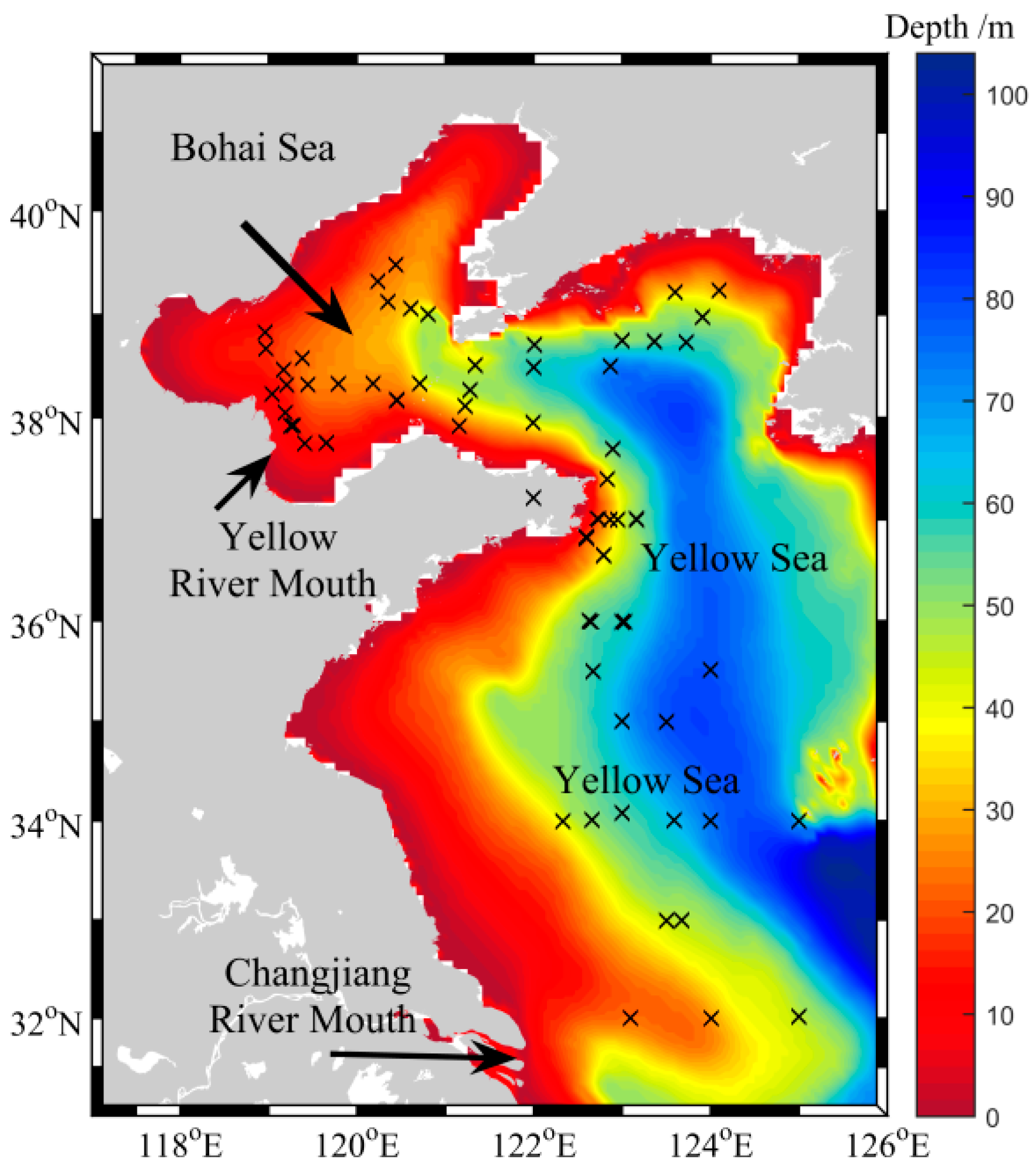
2.1. Study Area and Sampling

The data used in this study were collected during three cruises in May 2014, November 2014 and August 2015 in the BS and the YS aboard the R/V Dongfanghong 2 (Figure 1). The BS is known as a shallow (average depth of 18 m) and highly productive inner sea of China [19]. A notably large amount of mineral-rich particles carried by the Yellow River flows into the BS. Additionally, in the past several decades, the BS has been strongly impacted by human activities because of the rapid proliferation of surrounding industries, agriculture, aquaculture and domestic sewage [19]. The YS is one of the largest marginal seas in the western North Pacific, with an area of 380,000 km2 and an average water depth of 44 m. The YS is semi-enclosed by the contiguous lands of China in the west and Korea in the east and is connected with the BS through the Bohai Strait. Because of freshwater discharge from inland rivers carrying abundant nutrients and sediments and water mixing driven by winds and tides, water properties in the YS are regionally and seasonally varied over a wide dynamic range [20,21]. In addition, the YS is influenced by industrial pollution, agricultural runoff, and domestic sewage [21].
At each sampling station, a profiling package was used to measure various water properties. This package includes a Sequoia Scientific LISST-100X (type C) for determining the particle size distribution (PSD), a Seabird SBE911P conductivity-temperature-depth (CTD) profiler for measuring the hydrological characteristics of the water column, and other optical instruments (i.e., a WET labs AC-S and a HOBI Labs Hydroscat-6) used to determine the inherent optical properties of water. The profiling package was immersed in surface waters for several minutes to equilibrate the sensor temperature and the seawater temperature, and was subsequently slowly (0.2 m·s−1) lowered from the surface to 2–3 m above the bottom to measure a vertical profile. We used only downcast measurements for data analysis to avoid perturbations of the package on the water column. At the daytime stations, a Satlantic Hyper-Profiler II radiometer was used to derive Rrs(λ). Similarly, this instrument was also stabilized at the surface water for several minutes to reduce the influence of temperature differences between sensor and water. This process also allowed the instrument to drift further away from the ship to avoid the ship’s shadow. Using a hand-controlled cable, we lowered the instrument from the surface in vertical free-fall mode until it reached the euphotic layer, which is defined as the depth with 1% surface photosynthetically active radiation [22]. The downcast measurements were used in determining of Rrs(λ). In addition, surface water samples for measurement of TSM concentrations were simultaneously collected using 12-liter Niskin bottles mounted on a CTD/rosette system. In total, 86 surface samples with good quality were obtained that incorporated all measurements from the profiling package, Hyper-Profiler II and TSM concentrations.

2.2. In Situ Data Measurements

The cross-sectional area concentration AC values were calculated from field measurements of the volume scattering function using a LISST-100X Type-C particle size analyzer (Sequioa Scientific Inc., Bellevue, WA, USA). In brief, this instrument records the light scattering of particles at a wavelength of 670 nm at 32 logarithmically spaced scattering angles in the near-forward direction [10]. The volume concentrations with mean diameters of 32 particle size bins (range: 2.5–500 μm) are determined through inversion of the angular forward-scattering pattern based on Mie theory calculations [23]. By assuming the particles as spherical, the cross-sectional area concentration of particles of each size class was calculated as
AC i = 3 2 D i VC i ,
where ACi, Di and VCi denote the cross-sectional area concentration, mean diameter and volume concentration of particles in size bin i, respectively. As reported in previous studies [9,24], measurements from the LISST instrument usually show significant instability at the smallest and largest size ranges. These instabilities are possibly caused by the presence of particles that are smaller and larger than the measured size range and that of the smallest size ranges might also be associated with stray light [25]. Therefore, the data from the first and the last size bins, which respectively correspond to the smallest and the largest size ranges, were excluded from our analysis. The total cross-sectional area concentration AC was subsequently obtained as
AC = i = 2 31 AC i ,
where i ranges from 2 to 31 with corresponding values of 3.2 μm ≤ Di ≤ 390 μm.
Remote sensing reflectance Rrs(λ) values were determined using measurements from the Hyper-Profiler II (Satlantic Inc., Halifax, NS, Canada). This instrument includes three inter-calibrated radiometers, i.e., a deck sensor that measures the above-water surface downwelling irradiance (Ed(λ, 0+)) and two underwater sensors that respectively measure the vertical profiles of downwelling irradiance (Ed(λ, z)) and upwelling radiance (Lu(λ, z)). These measured spectra range from 349 to 804 nm with a mean bandwidth of approximately 3.3 nm. The radiometric measurements were processed to perform calibration, data filtering, binning and interpolation using the manufacturer-provided software Prosoft 7.7.16 [26]. Data with tilt angles >5° or/and downward velocity >0.5 m·s−1 were excluded during the processing, and Rrs(λ) was obtained as
R rs ( λ ) = L w ( λ ) E d ( λ , 0 + ) ,
where Lw(λ) is the water-leaving radiance determined from the profile of Lu(λ, z) at the upper layer, as described by Rudorff et al. [26].
In this study, we intended to investigate the utility of ocean color measurements for retrieval of AC. Recently, the Geostationary Ocean Color Imager (GOCI), the world’s first geostationary ocean color satellite sensor, has become increasingly popular due to its high temporal resolution. GOCI observes the Northeast Asian region 8 times within a day from 8:15 to 15:15 local time (temporal resolution of 1 h). In the visible region, GOCI contains 6 bands with central wavelengths of 412, 443, 490, 555, 660 and 680 nm. Therefore, in this study, we resampled the in situ hyper-spectral Rrs(λ) to the GOCI bands based on the spectral response function.
TSM concentrations were determined gravimetrically by filtration of 0.5–2 L of seawater onto 47-mm Whatman GF/F glass fiber filters [27]. These filters were pre-weighed on a balance with an accuracy of 0.01 mg and stored in a desiccator before the cruise. Water samples were filtered onto the pre-weighed filters under low vacuum pressure (<0.01 MPa). After filtration, the filters were rinsed three times using 50 mL MilliQ water to remove immersed salt and immediately frozen at −20 °C before drying at 105° for 4 h in the laboratory. The filters were reweighed on a balance to obtain the TSM concentrations until the difference between the last two measurements was within 0.02 mg. The TSM concentrations were corrected for the sea salt plus water of hydration retention using the method proposed by Stavn et al. [28]. The salinity data used for the correction was from the CTD measurements.

2.3. Satellite Data

Level 1B products of top-of-atmosphere radiance of GOCI (with 8 images per day) in 2015 and during our cruise period in 2014 were obtained from the Korea Ocean Satellite Center (KOSC). These products were cropped to the BS and the YS and processed to Level 2 data for Rrs(λ) using the GOCI Data Processing Software (GDPS, version 1.3) set to the default parameters and standard atmospheric correction [29]. Subsequently, to derive the monthly variations of AC in the BS and the YS, we produced monthly Rrs(λ) in 2015 from the hourly Level 2 Rrs(λ) using the combined time-series tool of GDPS.

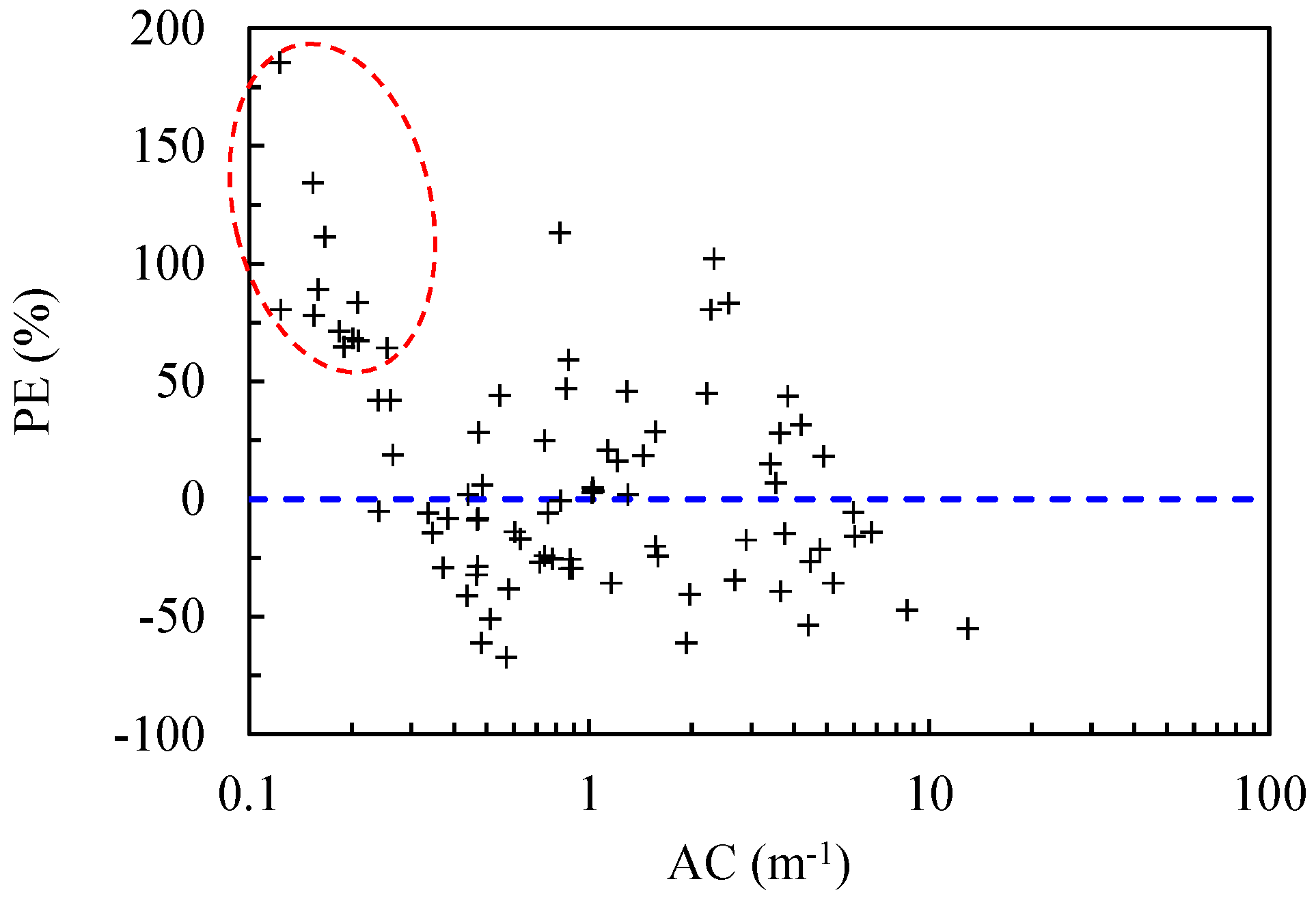
2.4. Accuracy Assessment

The performance of the AC estimation model proposed in this study was assessed with comparison between the Rrs(λ)-retrieved AC and those measured values [30]. The coefficient of determination R2 calculated in the log-log space was used to show how well the derived AC agreed with the measured values. Two other indicators, the root mean squared error (RMSE) and the mean absolute percentage error (MAPE), were also used to demonstrate the scatter between the measured and estimated values, which were calculated as follows [31]:
RMSE = 1 N i = 1 N [ y est , i y mea , i ] 2
MAPE = 1 N i = 1 N | y est , i y mea , i y mea , i | × 100 %
where yest,i and ymea,i represent the estimated and measured AC for the ith sample, respectively, and N is the total number of samples.

3. Results

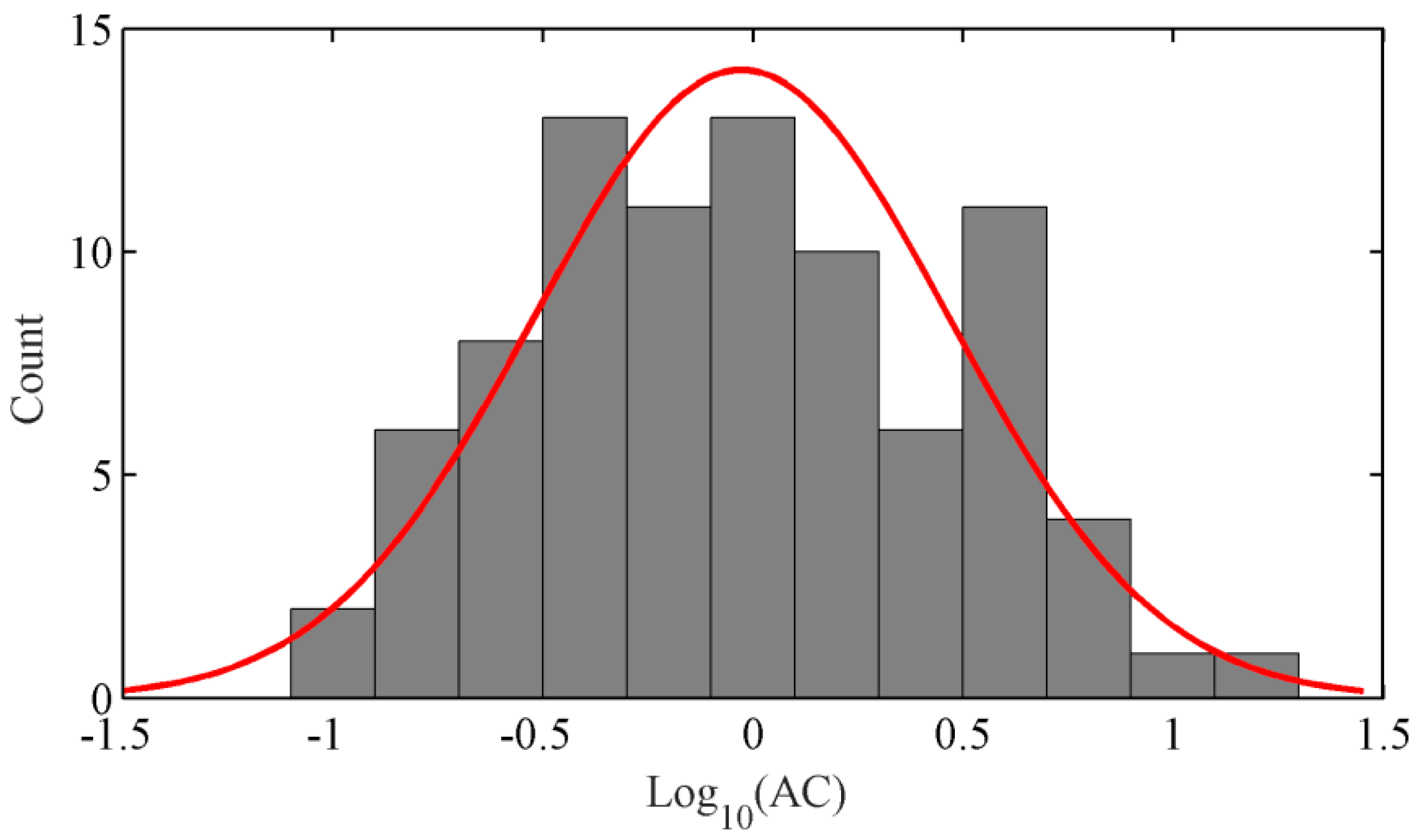
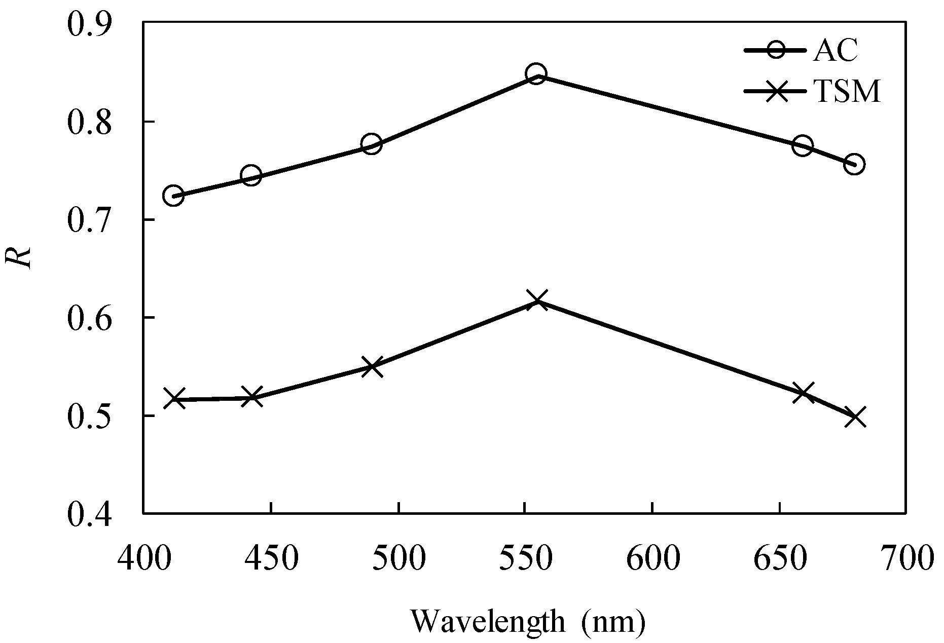
3.1. Data Distributions

The particle concentrations showed wide dynamic ranges and significant variability (Table 1). The TSM varied from 0.53 to 43.88 g·m−3 with a mean value of 7.60 g·m−3 (standard variation of 7.25 g·m−3). The variation coefficient of TSM was 95.4%. Compared with TSM, the AC showed more significant variation with a range from 0.12 to 13.00 m−1. The values for the mean, standard variation and variation coefficient of AC were 1.74 m−1, 2.14 m−1 and 123.0%, respectively. In general, the AC was log-normally distributed, as shown in Figure 2.
Correspondingly, the remote sensing reflectance Rrs(λ) values of all samples showed large variations in both magnitude and spectral shape, although the spectral shapes generally appeared similar (Table 1 and Figure 3). The spectral variability in magnitude and shape of Rrs(λ) were generally in accord with those reported in previous studies in coastal regions [32,33]. For the majority of samples, the Rrs(λ) spectra displayed peaks between 550 and 600 nm, whereas the spectral peaks of some samples mainly collected from offshore waters of the Bohai Strait and YS during late summer and autumn were shifted to around 490 nm. The in situ hyper-spectral Rrs(λ) were resampled to the GOCI 6 bands according their spectral response functions. The statistics of synthetic GOCI Rrs(λ) at 6 bands were summarized in Table 1.

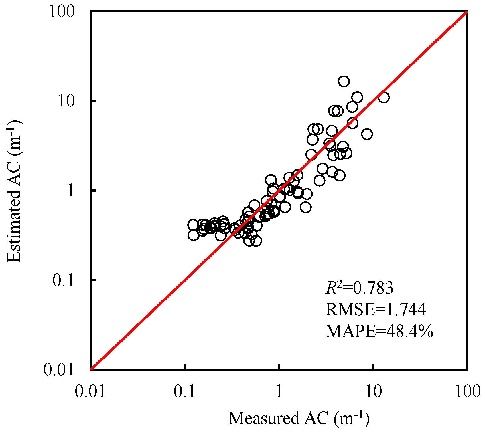
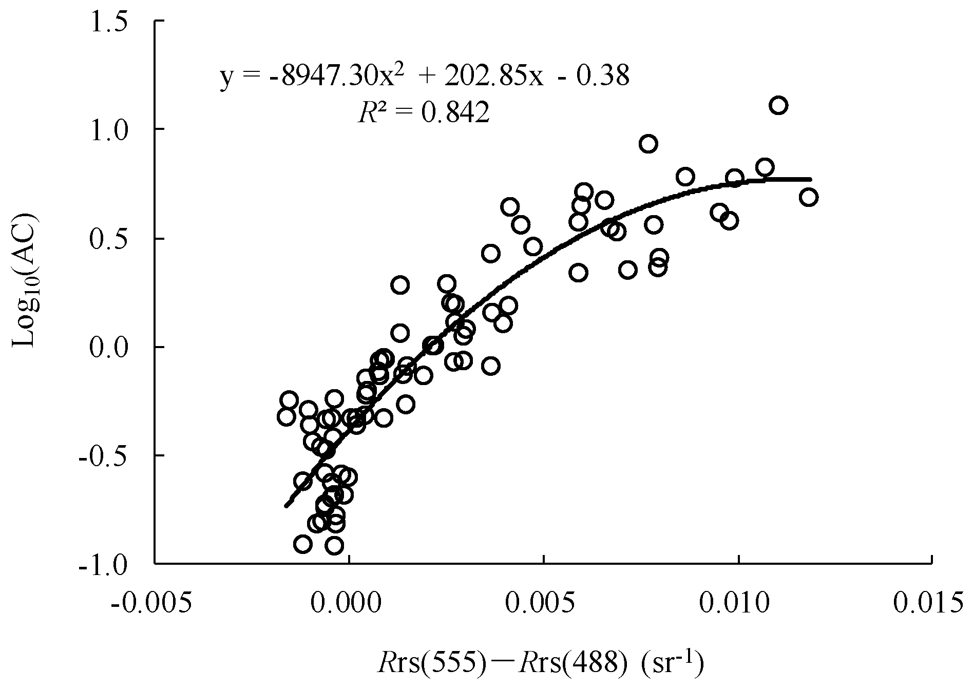
3.2. Development and Performance of AC Retrieval Model

Before the model development, we analyzed the relationship between Rrs(λ) and AC, and compared with those between Rrs(λ) and TSM. Considering the log-normal distribution of AC (Figure 2), the correlations of log-transformed AC (log10(AC)) with Rrs(λ) were analyzed for each band of GOCI. The highest correlation between log10(AC) and Rrs(λ) was found at 555 nm with a value of 0.85 (Figure 4). The second highest correlations occurred at 490 and 660 nm with values of 0.77 and 0.77, respectively. We also analyzed the correlation between log10(TSM) and Rrs(λ). Although the variation pattern of the correlations along the wavelength between log10(TSM) and Rrs(λ) was similar to that between log10(AC) and Rrs(λ), the values of the correlations between log10(TSM) and Rrs(λ) were much lower, with the highest correlation of only 0.62 at 555 nm. The causes of these differences are discussed later in Section 4.2.
Empirical models have been widely used to derive water quality parameters [34,35] because of their simple and easy implementation. Considering the log-normal distribution and the above correlation analysis, we designed an empirical model for retrieval of AC from Rrs(λ), the general form of which can be expressed as
log 10 ( A C ) = k 1 X 2 + k 2 X + k 0
where X represents the spectral indicator constructed from Rrs(λ), and k0, k1, and k2 are model parameters that can be derived by regression analysis. This general form of the retrieval model for AC is similar to that used for TSM in previous studies, and single band, band ratios and band arithmetic calculations are often used in the spectral indicator X [36,37,38]. In this study, we designed four forms of X to derive the best model for estimating AC. Regarding the four forms, X1 and X2 represent the single band and band ratio, respectively; X3 denotes the difference of Rrs(λ) at two bands; and X4 represents the arithmetic calculation of Rrs(λ), which was referred from the spectral form used for estimation of TSM [34] (Table 2).
For each spectral indicator X, its ability for estimating AC was examined for all possible combinations from GOCI 6 Rrs(λ) bands. The best band combinations that displayed the highest R2 and the lowest RMSE and MAPE for estimation of AC are shown in Table 2. Among the four types of spectral indicator, X3 indicating the difference of Rrs(λ) between 490 and 555 nm showed the best performance, and the performance of X1 representing the single band of Rrs(λ) at 555 nm was the worst. The X2 and X4 showed slightly poorer ability than X3. Therefore, we recommend X3 as the best spectral indicator for estimation of AC from Rrs(λ) and decided to use it in our model. The fitting plots between log10(AC) and X3 are shown in Figure 5. It can be observed that most of the samples cluster around the fitting curve with an R2 value of 0.843. Comparisons between the measured AC and estimated values for the same dataset also showed good agreement with RMSE and MAPE values of 1.145 m−1 and 38.9%, respectively (Table 2).
Note that the model fitting of this study was based on the log-transformed AC data, while the fitting can also be conducted directly based on untransformed data. We have compared the two manners for the model fitting, the results indicated that the model based on log-transformed AC data generally performed better than the model based on untransformed data (data not shown), probably because that log-transformation may reduce uncertainty of outliers to some extent. Thus, the log-transformed AC data are recommended to use for model calibration.
To further evaluate the performance and test the robustness of the AC estimation model, we conducted a cross-validation [39]. In brief, one sample was selected from the full dataset, which was used in model validation. The remaining samples were used in model calibration, and the calibrated model was adapted to derive the AC for the remaining one sample. This procedure was repeated until all of the samples of the full dataset were selected as the validation sample. The estimated AC values obtained from the above steps were independent of each other and formed a new validation dataset. Subsequently, comparisons were performed between these estimated AC and the measured values, and R2, RMSE and MAPE were calculated. As shown in Figure 6, a strong linear relationship was found between the estimated AC and measured values in logarithmic space, with values of R2, RMSE and MAPE of 0.783, 1.744 m−1 and 48.4%, respectively.

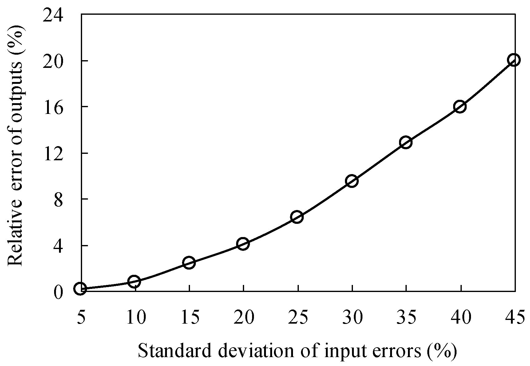
3.3. Model Sensitivity Analysis

The sensitivities of the developed models to the uncertainties in Rrs(λ) were examined. We added random errors with a standard deviation of m and average value of 0 to the spectral indicator X3 (i.e., the difference of Rrs(λ) between 490 or 555 nm) of all samples. This process was repeated 1000 times; thus an approximately normal distribution was produced in the added random errors. The mean of the relative errors in the estimated AC compared with those derived from Rrs(λ) without addition of errors was subsequently calculated by averaging the errors across the 1000 repetitions. Considering the uncertainty in X3 may reach around 40% for GOCI satellite measurements as shown in Figure 8 later, we varied the standard deviation m of the errors from 5% to 45% with an interval of 5% and conducted the above procedure for each value of m.
As shown in Figure 7, it was found that the relative errors in the estimations of AC increased with increases in the random errors added to spectral indicator X3, and the increase rate gradually became large. Note that although the relative errors in the estimations of AC gradually became large with the increases of the uncertainty in X3, when 45% random errors were added to X3, the relative errors yielded by the model was 20.1%. These results indicate that the AC estimation model is robust for input errors.

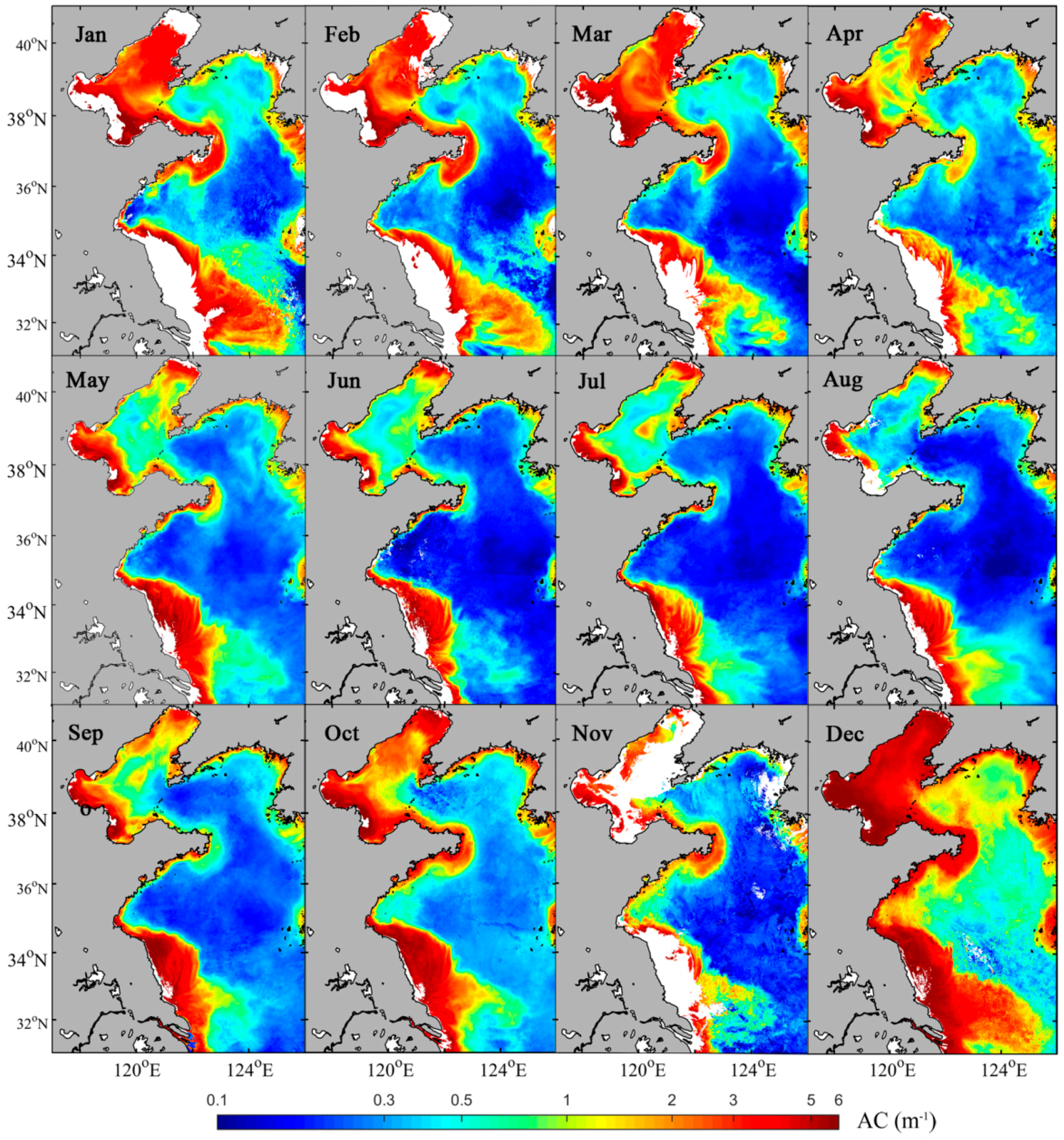
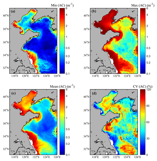
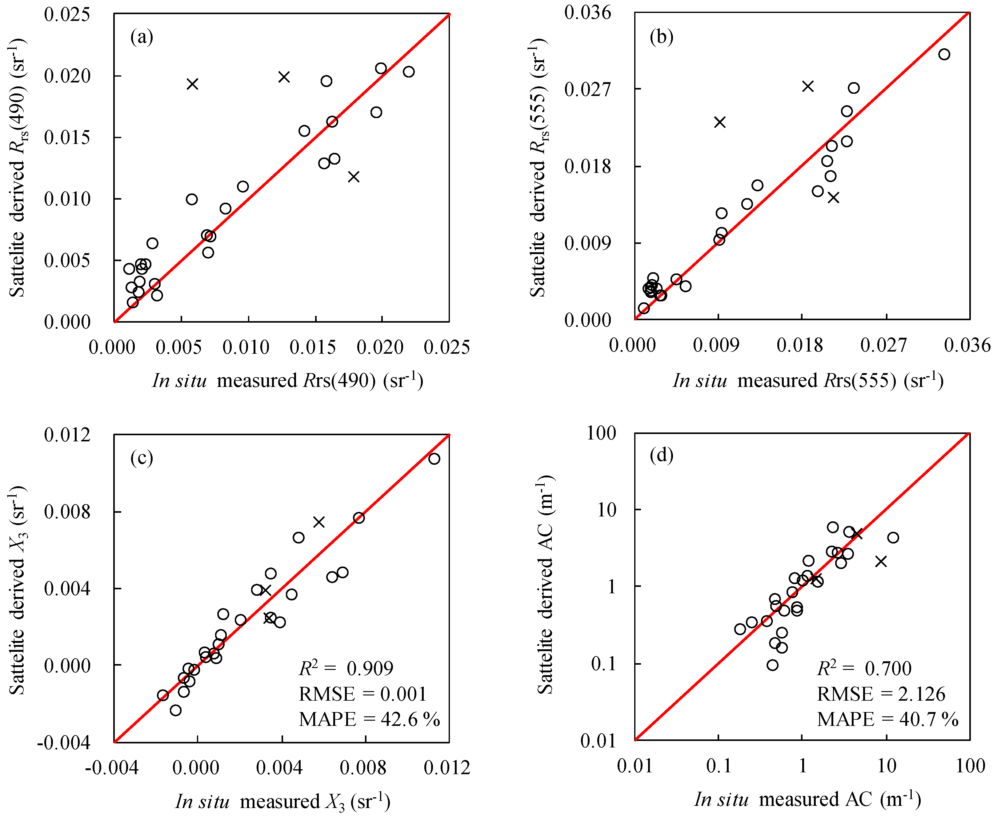
3.4. Model Application to Satellite Data

We applied the developed AC retrieval model to the GOCI satellite data to preliminarily investigate the spatial and temporal variations of AC in the BS and the YS. Before the application, the satellite derived Rrs(λ) and the performance of the AC retrieval model for satellite Rrs(λ) was validated based on a dataset containing 28 pairs of in situ measurements and GOCI satellite data. This match-up dataset only included satellite Rrs(λ) with an overpass time within 3 h before and after field measurements [30,40,41]. To avoid the influences of outliers, the median Rrs(λ) values from a 3 × 3 pixel window centered on the locations of the field sampling stations were used as GOCI satellite Rrs(λ). In general, satellite derived Rrs(490) and Rrs(555) of the most samples showed good agreement with in situ measured values, while large errors were also observed for some samples (marked by crosses) (Figure 8a,b). However, note that the model of this study uses the spectral indicator X3 (i.e., the difference between Rrs(555) and Rrs(490)) rather than the single band. We found that although these samples showed large errors in satellite Rrs(λ), X3 of them were consistent with in situ measured values (Figure 8c). Subsequently, these 28 satellite Rrs(λ) were used to derive AC by the model which was calibrated based on the remaining subset (N = 58) of the full 86 in situ measurements (independent of validation dataset). As shown in Figure 8d, the satellite-derived AC generally agreed well with field measured AC, with values of R2, RMSE and MAPE of 0.700, 2.126 m−1 and 40.7%, respectively. These results suggest that our model has good performance for satellite application of GOCI data.
The distributions of the AC estimated from composited GOCI monthly Rrs(λ) were shown in Figure 9 and Figure 10. Clear spatial and temporal variations of AC were observed in the BS and the YS (Figure 9). In general, the AC of coastal shallow waters showed much higher values than those in offshore waters, while variations of the AC in coastal regions were lower compared with those in offshore waters (Figure 10). The high AC in the Yellow River mouth and the Changjiang River mouth and their adjacent regions might be related to sediment loads from these rivers, and the high AC in other coastal regions is possibly associated with re-suspension of particles driven by tidal mixing and/or wind stress [42,43]. For offshore waters, the AC in the BS is higher than in the YS. At the temporal scale, the AC was the lowest in summer in most regions of the BS and the YS, whereas in winter, the AC showed the highest values, especially in December. During spring and autumn, high values of AC were observed in offshore waters. The lowest and the highest AC during summer and winter might be related to water stratification and strong mixing, respectively, and the high AC in spring and autumn in offshore waters is possibly caused by algae bloom [20,44]. Understanding the controlling factors of the spatial and temporal variability in AC is beyond the scope of this study, but this topic will be further investigated. However, as mentioned above, re-suspension of particles, sediment loads from rivers and water mixing are possible causes. Meanwhile, we note that some coastal regions in images show invalid pixels (white color). These invalid pixels are mainly related to the effects of unsuccessful atmospheric correction. In this study, we used the standard atmospheric correction method to process GOCI data, by which turbid waters are often masked. Atmospheric correction in coastal regions has been a difficult point for ocean color remote sensing for a long time. Further efforts focusing on this issue are still required.

4. Discussion

4.1. Rationality and Limitation of AC Retrieval Model

Suspended matters significantly impact the underwater light field, algae photosynthesis and the ocean color signal through light absorption and scattering processes [3,4]. Theoretical, experimental and in situ studies have proved that the inherent optical properties of suspended particles are more sensitive to AC than TSM [6,11,12,15] because of the direct dependences of the chance of a photon interacting with a particle on cross-sectional area rather than mass [7]. Consequently, remote sensing reflectance Rrs(λ) as a function of light absorption and backscattering is also more strongly related to AC than TSM [7,8,18]. In this study, as expected, our analysis showed that although the AC varied over a large range, the correlations between AC and Rrs(λ) at six bands of GOCI were strong and were approximately 1.4 times higher than those between Rrs(λ) and TSM (Figure 4). The strong relationship between AC and the inherent optical properties, thus Rrs(λ), offers a solid optical basis for deriving AC from Rrs(λ).
The retrieval model of AC was empirically determined by comparing the performances of four types of spectral indicators constructed from all possible GOCI satellite band combinations. The difference between Rrs(λ) at 490 and 555 nm, which in fact represents the slope of Rrs(λ) between these two bands, is recommended as the best spectral indicator for estimation of AC (Table 2 and Figure 5). This observation is consistent with our correlation analysis, which indicated that these two bands showed the highest correlations with the AC (Figure 4). The model sensitivity analysis suggests that our model is robust for uncertainties in Rrs(λ) (Figure 7). In general, the AC retrieval model is simple and can be easily implemented in other regions as well as in other ocean color sensors, such as the Sea-viewing Wide Field-of-view Sensor (SeaWiFS), the Moderate Resolution Imaging Spectroradiometer (MODIS) and the Medium Resolution Imaging Spectrometer (MERIS) because bands similar to 490 and 550 nm are commonly set for most of the ocean color sensors. This was confirmed when we derived a retrieval model of AC for MODIS based on a synthetic dataset of MODIS Rrs(λ) using the same approach as that for GOCI. We found that for MODIS, the difference between Rrs(555) and Rrs(488) was also the best for deriving the AC, and the model performances were comparable to those of the model for GOCI, with R2, RMSE and MAPE values of 0.842, 1.146 m−1 and 38.9%, respectively (Figure 11). However, due to the lack of sufficient match-ups of MODIS satellite data and in situ measurements, currently it is difficult to evaluate the performance of the algorithm for real MODIS satellite data.
It was noted that the data used in this study were collected mainly from coastal regions, and a subset even originated from turbid waters, showing mean values of TSM and AC of 7.60 g·m−3 and 1.74 m−1, respectively, and the highest values reached 43.88 g·m−3 and 13.00 m−1, respectively (Table 1). These results imply that the model developed in this study might be mostly suitable for coastal regions. We verified this speculation by analyzing the distribution of the percentage errors (PE) in estimations of AC. As shown in Figure 12, when the AC was larger than 0.20 m−1, our model performed well, showing that the PE were uniformly distributed around the two sides of the 0% line with a mean absolute value of 30.9%. At a notably low AC range (AC < 0.20 m−1), the samples showed significant estimation errors, with PE >50%, and the PE values of these samples were positive, indicating overestimations in AC. However, it was noted that the samples were few (N = 11). A future hybrid model applicable for both coastal and clear waters, and particularly for clear waters, might further improve the accuracy in estimations of AC, but it is difficult to conduct such an analysis at this stage because of limited samples from clear waters in our dataset. In addition, bio-optical properties of particles in coastal regions are complex and dynamic due to changes in particle assemblages [45]. Although the algorithm of this study performed generally well in the BS and YS, its applicability in additional coastal regions must be validated in further investigations.
The AC estimation model proposed in this study uses the difference between Rrs(550) and Rrs(490). It is known that Rrs(λ) is regulated by the absorption of pure seawater, particles and colored dissolved organic matter (CDOM), and the backscattering of pure seawater and particles [46]. Usually, absorption and backscattering coefficients of pure seawater are treated as constant values [46]. In this sense, changes in the absorption of CDOM may impact the AC estimation model, since although the absorption of CDOM at 490 and 555 nm is usually low, it should not be ignored. Due to the lack of in situ measurements of CDOM, we could not exactly examine to what extent CDOM would impact the AC estimation model. The in situ data used in this study collected from large regions covering river-influenced coastal waters and offshore waters, in which CDOM might vary greatly, while the AC model performed generally well. This observation implies that the AC estimation model may be generally robust to CDOM in the BS and YS, while further investigations are required based on available CDOM measurements.
It should be noted that the AC data used in this study were determined from LISST measurements. Due to the inherent limitation of LISST instrument, the AC data only account for information of particles within the size range of 3.2–390 μm. Risović [47] showed that sub-micron particles may have significant contribution to backscattering signal, so that the particles measured by LISST may not appropriately explain changes in bbp(λ) and Rrs(λ) as well. However, in our previous studies conducted in the BS and YS [15], we found that more than 90% of variability in bbp(λ) could be explained by the AC of particles measured by LISST. Therefore, although LISST measurements only effectively cover a size range of 3.2–390 μm, we believe in our study region, the AC values derived from LISST measurements can effectively explain variations in optical properties. In addition, to describe the relationship between AC and optical properties, particles are usually assumed to be spherical. This assumption is useful and has been widely used in studies of bio-optical properties of particles [9,13,16,48], while we have to admit that this assumption may be not necessarily valid in natural environments, which may bring uncertainty in the relationship between AC and optical properties described in this study. Therefore, regarding the above two issues, more advanced field instruments that can cover larger particle size ranges and reveal more adequate particle shapes should be developed in future that will facilitate development of a more accurate AC estimation model.

4.2. Implications of Remote Sensing Applications of AC

The cross-sectional area of suspended particles is a key factor to link the suspended particles with their optical properties. Satellite derived AC using the model proposed in this study provide a new property of suspended particles from space, which may improve our understanding of particle biogeochemical properties and the role of particles in determination of water optical properties. First of all, AC is closely related to the inherent optical properties (i.e., attenuation, scattering and backscattering coefficients) as shown in Equation (1) for the backscattering coefficient as an example, and the relationships are often observed to be strong [11,12,15]. This observation indicates that the inherent optical properties can be modeled from AC with knowledge of the corresponding efficiency factors. Additionally, because the chances of photons interacting with particles directly depend on the cross-sectional area, the light conditions underwater might also be estimated based on the information about AC. In our dataset, strong correlation between AC and transparency (R2 = 0.87) in log-log space was observed, implying that AC retrieved from satellite observations using our model might have great potential for mapping transparency and photosynthetically active radiation, which is important for phytoplankton photosynthesis.
Inherent optical properties are linked with AC by efficiency factors. Many field investigations have observed clear differences in attenuation and backscattering efficiencies among different particle compositions (e.g., phytoplankton and mineral particles) [9,15,48,49,50,51]. For instance, Vaillancourt et al. [50] showed that Qbbe(λ) levels at 620 nm for cultured 28 phytoplankton species varied from 0.001 to 0.068 with a mean of 0.011; and Peng and Effler [51] found that Qbbe(λ) levels at 650 nm of mineral particles ranged from 0.046 to 0.062 with a median value of 0.051. Particularly, Bowers et al. [48] observed a strong positive relationship between Qbbe(665) and particle composition (the ratio of minerals to total suspended matters) (R2 = 0.62), implying that Qbbe(665) might be used to detect particle composition. Similarly, in the BS and the YS, Wang et al. [15] found that Qbbe(640) clearly classified particles into two types respectively dominated by organic or relatively large particles and small mineral particles. As shown in this study, AC can be successfully derived from satellite measurements using the model developed in this work. At the same time, values of bbp(λ) can also be retrieved from satellite Rrs(λ) using an inherent optical properties algorithm [52,53]. Consequently, Qbbe(λ) can be easily calculated as the ratio of bbp(λ) to AC. When satellite Qbbe(λ) data become available, particle composition or particle classification might be mapped based on the findings of previous studies [15,48], and specific studies focusing on this topic are expected in future.
Although TSM has been widely used to quantify the amount of particles, and various remote sensing algorithms have been developed to map TSM from satellite measurements [27,54,55,56,57], the correlation of the inherent optical properties with TSM is weaker compared with AC. This may cause an unstable relationship between TSM and Rrs(λ), and thereby bring large errors in TSM estimations which could reach a factor of 10 if their values are derived from satellite measurements [8,18,58]. The reason for the large uncertainties is attributed to the fact that Rrs(λ) reflects the information not only for TSM but also for particle size distribution and density which might also vary by up to several orders of magnitude from location to location due to changes in particle composition and flocculation [13,59]. However, because of a more direct relationship between AC and Rrs(λ), retrieval of AC from Rrs(λ) suffers fewer influences from changes in particle size distribution and density. The relationship between TSM and AC can be approximately expressed as [7,9].
TSM = 2 AC 3 ρ a D A
This implies that satellite derived AC might offer an alternative approach for mapping of TSM. However, at this stage, it is important to note that estimation of TSM from AC also requires additional information on particle size and density, which is beyond of the scope of this study. Meanwhile, it is still needed to further evaluate whether this approach can improve the estimation of TSM.

5. Conclusions

The cross-sectional area of suspended particles is of fundamental importance for understanding water optical properties. Based on in situ measurements conducted in the Bohai Sea (BS) and the Yellow Sea (YS), this study proposed an algorithm for deriving concentration of particle cross-sectional area (AC) from GOCI satellite measurements. The designed algorithm uses the slope of the remote sensing reflectance Rrs(λ) between 490 and 555 nm as an input. Both in situ and satellite validations indicated that the algorithm shows good performances, with the R2 values of 0.783 and 0.700, RMSE values of 1.744 and 2.126 m−1 and MAPE values of 48.3% and 40.7%, respectively. This result indicates the great potential of the algorithm for mapping of AC from satellite measurements, which was confirmed by the generally reasonable patterns of the temporal and spatial distributions of AC derived using the new algorithm in the BS and the YS. Overall, this study provides a technological basis for estimation of AC from satellite measurements in the BS and the YS, and it may be easily implemented in other regions and for other ocean color sensors, while further investigations are required. The values of AC derived from satellite measurements might offer new potential applications of ocean color, such as modeling of the inherent optical properties of particulates, deriving water transparency, estimating particle composition and possibly improvement in the concentration estimations of total suspended particles, topics that will be specifically studied in future work.

Acknowledgments

Special thanks to Shuguo Chen and other members of the group led by Tinglu Zhang in Ocean University of China, other members of the group led by Zhongfeng Qiu in Nanjing University of Information Science & Technology and the captains, officers, and crews of R/V Dongfanghong 2 for their significant contributions on field sampling and measurements. We also would like to thank the anonymous reviewers for their constructive comments towards improving this manuscript. This work is jointly supported by the National Natural Science Foundation of China (NSFC) (41506200, 41276186, 41576172), the Natural Science Foundation of Jiangsu Province (BK20150914, BK20151526), the National Key Research and Development Program of China (2016YFC1400901, 2016YFC1400904), the Natural Science Foundation of the Jiangsu Higher Education Institutions of China (15KJB170015), the Priority Academic Program Development of Jiangsu Higher Education Institutions (PAPD), the Public Science and Technology Research Funds Projects of Ocean (201005030), the Startup Foundation for Introducing Talent of NUIST (2015r007), the National Programme on Global Change and Air-sea Interaction (GASI-03-03-01-01), the Priority Academic Program Development of Jiangsu Higher Education Institutions (PAPD), the Public Science and Technology Research Funds Projects of Ocean (201005030), and sponsored by Qing Lan Project.

Author Contributions

Shengqiang Wang designed this study and the algorithm; Yu Huan contributed to the data analyses and drafted the manuscript; Zhongfeng Qiu, Deyong Sun and Hailong Zhang assisted with developing the research design and results interpretation; Lufei Zheng and Cong Xiao contributed to the interpretation of results and manuscript revision.

Conflicts of Interest

The authors declare no conflict of interest.

References

  1. Doxaran, D.; Froidefond, J.-M.; Castaing, P.; Babin, M. Dynamics of the turbidity maximum zone in a macrotidal estuary (the Gironde, France): Observations from field and MODIS satellite data. Estuar. Coast. Shelf Sci. 2009, 81, 321–332. [Google Scholar] [CrossRef]
  2. Anderson, R.F.; Hayes, C.T. Characterizing marine particles and their impact on biogeochemical cycles in the geotraces program. Prog. Oceanogr. 2015, 133, 1–5. [Google Scholar] [CrossRef]
  3. Morel, A. Optics of marine particles and marine optics. In Particle Analysis in Oceanography; Demers, S., Ed.; Springer: Berlin, Germany, 1991; pp. 141–188. [Google Scholar]
  4. Babin, M.; Morel, A.; Fournier-Sicre, V.; Fell, F.; Stramski, D. Light scattering properties of marine particles in coastal and open ocean waters as related to the particle mass concentration. Limnol. Oceanogr. 2003, 48, 843–859. [Google Scholar] [CrossRef]
  5. Gordon, H.R.; Morel, A.Y. Remote Assessment of Ocean Color for Interpretation of Satellite Visible Imagery: A Review; Springer: Berlin, Germany, 1983; Volume 4. [Google Scholar]
  6. Mobley, C.D. Light and Water: Radiative Transfer in Natural Waters; Academic Press: Cambridge, MA, USA, 1994. [Google Scholar]
  7. Bowers, D.; Braithwaite, K. Evidence that satellites sense the cross-sectional area of suspended particles in shelf seas and estuaries better than their mass. Geo-Mar. Lett. 2012, 32, 165–171. [Google Scholar] [CrossRef]
  8. Mikkelsen, O.A. Variation in the projected surface area of suspended particles: Implications for remote sensing assessment of TSM. Remote Sens. Environ. 2002, 79, 23–29. [Google Scholar] [CrossRef]
  9. Neukermans, G.; Loisel, H.; Mériaux, X.; Astoreca, R.; McKee, D. In situ variability of mass-specific beam attenuation and backscattering of marine particles with respect to particle size, density, and composition. Limnol. Oceanogr. 2012, 57, 124–144. [Google Scholar] [CrossRef]
  10. Agrawal, Y.; Pottsmith, H. Instruments for particle size and settling velocity observations in sediment transport. Mar. Geol. 2000, 168, 89–114. [Google Scholar] [CrossRef]
  11. Hatcher, A.; Hill, P.; Grant, J. Optical backscatter of marine flocs. J. Sea Res. 2001, 46, 1–12. [Google Scholar] [CrossRef]
  12. Flory, E.; Hill, P.; Milligan, T.; Grant, J. The relationship between floc area and backscatter during a spring phytoplankton bloom. Deep Sea Res. Part I Oceanogr. Res. Pap. 2004, 51, 213–223. [Google Scholar] [CrossRef]
  13. Boss, E.; Slade, W.; Hill, P. Effect of particulate aggregation in aquatic environments on the beam attenuation and its utility as a proxy for particulate mass. Opt. Express 2009, 17, 9408–9420. [Google Scholar] [CrossRef] [PubMed]
  14. Bowers, D.; Braithwaite, K.; Nimmo-Smith, W.; Graham, G. The optical efficiency of flocs in shelf seas and estuaries. Estuar. Coast. Shelf Sci. 2011, 91, 341–350. [Google Scholar] [CrossRef]
  15. Wang, S.; Qiu, Z.; Sun, D.; Shen, X.; Zhang, H. Light beam attenuation and backscattering properties of particles in the Bohai Sea and Yellow Sea with relation to biogeochemical properties. J. Geophys. Res. Oceans 2016, 121, 3955–3969. [Google Scholar] [CrossRef]
  16. Bowers, D.; Braithwaite, K.; Nimmo-Smith, W.; Graham, G. Light scattering by particles suspended in the sea: The role of particle size and density. Cont. Shelf Res. 2009, 29, 1748–1755. [Google Scholar] [CrossRef]
  17. Kostadinov, T.S.; Siegel, D.A.; Maritorena, S. Retrieval of the particle size distribution from satellite ocean color observations. J. Geophys. Res. 2009, 114, C09015. [Google Scholar] [CrossRef]
  18. Bale, A.; Tocher, M.; Weaver, R.; Hudson, S.; Aiken, J. Laboratory measurements of the spectral properties of estuarine suspended particles. Neth. J. Aquat. Ecol. 1994, 28, 237–244. [Google Scholar] [CrossRef]
  19. Wei, H.; Sun, J.; Moll, A.; Zhao, L. Phytoplankton dynamics in the Bohai Sea—Observations and modelling. J. Mar. Syst. 2004, 44, 233–251. [Google Scholar] [CrossRef]
  20. Chen, C.-T.A. Chemical and physical fronts in the Bohai, Yellow and East China Seas. J. Mar. Syst. 2009, 78, 394–410. [Google Scholar] [CrossRef]
  21. Zhang, M.; Tang, J.; Song, Q.; Dong, Q. Backscattering ratio variation and its implications for studying particle composition: A case study in Yellow and East China Seas. J. Geophys. Res. Oceans 2010, 115. [Google Scholar] [CrossRef]
  22. Qiu, Z.; Wu, T.; Su, Y. Retrieval of diffuse attenuation coefficient in the china seas from surface reflectance. Opt. Express 2013, 21, 15287–15297. [Google Scholar] [CrossRef] [PubMed]
  23. Agrawal, Y.; Whitmire, A.; Mikkelsen, O.A.; Pottsmith, H. Light scattering by random shaped particles and consequences on measuring suspended sediments by laser diffraction. J. Geophys. Res. Oceans 2008, 113. [Google Scholar] [CrossRef] [Green Version]
  24. Traykovski, P.; Latter, R.J.; Irish, J.D. A laboratory evaluation of the laser in situ scattering and transmissometery instrument using natural sediments. Mar. Geol. 1999, 159, 355–367. [Google Scholar] [CrossRef]
  25. Reynolds, R.; Stramski, D.; Wright, V.; Woźniak, S. Measurements and characterization of particle size distributions in coastal waters. J. Geophys. Res. Oceans 2010, 115. [Google Scholar] [CrossRef]
  26. De Moraes Rudorff, N.; Frouin, R.; Kampel, M.; Goyens, C.; Meriaux, X.; Schieber, B.; Mitchell, B.G. Ocean-color radiometry across the southern atlantic and southeastern pacific: Accuracy and remote sensing implications. Remote Sens. Environ. 2014, 149, 13–32. [Google Scholar] [CrossRef]
  27. Miller, R.L.; McKee, B.A. Using MODIS Terra 250 m imagery to map concentrations of total suspended matter in coastal waters. Remote Sens. Environ. 2004, 93, 259–266. [Google Scholar] [CrossRef]
  28. Stavn, R.H.; Rick, H.J.; Falster, A.V. Correcting the errors from variable sea salt retention and water of hydration in loss on ignition analysis: Implications for studies of estuarine and coastal waters. Estuar. Coast. Shelf Sci. 2009, 81, 575–582. [Google Scholar] [CrossRef]
  29. Wang, M.; Gordon, H.R. A simple, moderately accurate, atmospheric correction algorithm for SeaWiFS. Remote Sens. Environ. 1994, 50, 231–239. [Google Scholar] [CrossRef]
  30. Hyde, K.J.; O’Reilly, J.E.; Oviatt, C.A. Validation of SeaWiFS chlorophyll a in Massachusetts Bay. Cont. Shelf Res. 2007, 27, 1677–1691. [Google Scholar] [CrossRef]
  31. Antoine, D.; d’Ortenzio, F.; Hooker, S.B.; Bécu, G.; Gentili, B.; Tailliez, D.; Scott, A.J. Assessment of uncertainty in the ocean reflectance determined by three satellite ocean color sensors (MERIS, SeaWiFS and MODIS-A) at an offshore site in the mediterranean sea (BOUSSOLE project). J. Geophys. Res. Oceans 2008, 113. [Google Scholar] [CrossRef]
  32. He, X.; Bai, Y.; Pan, D.; Huang, N.; Dong, X.; Chen, J.; Chen, C.-T.A.; Cui, Q. Using geostationary satellite ocean color data to map the diurnal dynamics of suspended particulate matter in coastal waters. Remote Sens. Environ. 2013, 133, 225–239. [Google Scholar] [CrossRef]
  33. Sun, D.; Hu, C.; Qiu, Z.; Cannizzaro, J.P.; Barnes, B.B. Influence of a red band-based water classification approach on chlorophyll algorithms for optically complex estuaries. Remote Sens. Environ. 2014, 155, 289–302. [Google Scholar] [CrossRef]
  34. Tassan, S. Local algorithms using seawifs data for the retrieval of phytoplankton, pigments, suspended sediment, and yellow substance in coastal waters. Appl. Opt. 1994, 33, 2369–2378. [Google Scholar] [CrossRef] [PubMed]
  35. O’Reilly, J.E.; Maritorena, S.; Mitchell, B.G.; Siegel, D.A.; Carder, K.L.; Garver, S.A.; Kahru, M.; McClain, C. Ocean color chlorophyll algorithms for SeaWiFS. J. Geophys. Res. Oceans 1998, 103, 24937–24953. [Google Scholar] [CrossRef]
  36. Doxaran, D.; Froidefond, J.-M.; Lavender, S.; Castaing, P. Spectral signature of highly turbid waters: Application with SPOT data to quantify suspended particulate matter concentrations. Remote Sens. Environ. 2002, 81, 149–161. [Google Scholar] [CrossRef]
  37. Mao, Z.; Chen, J.; Pan, D.; Tao, B.; Zhu, Q. A regional remote sensing algorithm for total suspended matter in the East China Sea. Remote Sens. Environ. 2012, 124, 819–831. [Google Scholar] [CrossRef]
  38. Siswanto, E.; Tang, J.; Yamaguchi, H.; Ahn, Y.-H.; Ishizaka, J.; Yoo, S.; Kim, S.-W.; Kiyomoto, Y.; Yamada, K.; Chiang, C. Empirical ocean-color algorithms to retrieve chlorophyll-a, total suspended matter, and colored dissolved organic matter absorption coefficient in the Yellow and East China Seas. J. Oceanogr. 2011, 67, 627–650. [Google Scholar] [CrossRef]
  39. Kohavi, R. A study of cross-validation and bootstrap for accuracy estimation and model selection. In Proceedings of the 14th International Joint Conference on Artificial Intelligence, Montreal, QC, Canada, 20–25 August 1995; Volume 14, pp. 1137–1145.
  40. Bailey, S.W.; Werdell, P.J. A multi-sensor approach for the on-orbit validation of ocean color satellite data products. Remote Sens. Environ. 2006, 102, 12–23. [Google Scholar] [CrossRef]
  41. Cui, T.; Zhang, J.; Groom, S.; Sun, L.; Smyth, T.; Sathyendranath, S. Validation of MERIS ocean-color products in the Bohai Sea: A case study for turbid coastal waters. Remote Sens. Environ. 2010, 114, 2326–2336. [Google Scholar] [CrossRef]
  42. Yang, S.Y.; Jung, H.S.; Lim, D.I.; Li, C.X. A review on the provenance discrimination of sediments in the Yellow Sea. Earth-Sci. Rev. 2003, 63, 93–120. [Google Scholar] [CrossRef]
  43. Jiang, W.; Pohlmann, T.; Sun, J.; Starke, A. SPM transport in the Bohai Sea: Field experiments and numerical modelling. J. Mar. Syst. 2004, 44, 175–188. [Google Scholar] [CrossRef]
  44. Xu, Y.; Ishizaka, J.; Yamaguchi, H.; Siswanto, E.; Wang, S. Relationships of interannual variability in SST and phytoplankton blooms with giant jellyfish (Nemopilema nomurai) outbreaks in the Yellow Sea and East China Sea. J. Oceanogr. 2013, 69, 511–526. [Google Scholar] [CrossRef] [Green Version]
  45. Braithwaite, K.; Bowers, D.; Smith, W.N.; Graham, G.; Agrawal, Y.; Mikkelsen, O. Observations of particle density and scattering in the Tamar Estuary. Mar. Geol. 2010, 277, 1–10. [Google Scholar] [CrossRef]
  46. Gordon, H.R.; Brown, O.B.; Evans, R.H.; Brown, J.W.; Smith, R.C.; Baker, K.S.; Clark, D.K. A semianalytic radiance model of ocean color. J. Geophys. Res. Atmos. 1988, 93, 10909–10924. [Google Scholar] [CrossRef]
  47. Risović, D. Effect of suspended particulate-size distribution on the backscattering ratio in the remote sensing of seawater. Appl. Opt. 2002, 41, 7092–7101. [Google Scholar] [CrossRef] [PubMed]
  48. Bowers, D.; Hill, P.; Braithwaite, K. The effect of particulate organic content on the remote sensing of marine suspended sediments. Remote Sens. Environ. 2014, 144, 172–178. [Google Scholar] [CrossRef]
  49. Ahn, Y.-H.; Bricaud, A.; Morel, A. Light backscattering efficiency and related properties of some phytoplankters. Deep Sea Res. Part I Oceanogr. Res. Pap. 1992, 39, 1835–1855. [Google Scholar] [CrossRef]
  50. Vaillancourt, R.D.; Brown, C.W.; Guillard, R.R.; Balch, W.M. Light backscattering properties of marine phytoplankton: Relationships to cell size, chemical composition and taxonomy. J. Plankton Res. 2004, 26, 191–212. [Google Scholar] [CrossRef]
  51. Peng, F.; Effler, S.W. Characterizations of individual suspended mineral particles in Western Lake Erie: Implications for light scattering and water clarity. J. Gt. Lakes Res. 2010, 36, 686–698. [Google Scholar] [CrossRef]
  52. Lee, Z.; Carder, K.L.; Arnone, R.A. Deriving inherent optical properties from water color: A multiband quasi-analytical algorithm for optically deep waters. Appl. Opt. 2002, 41, 5755–5772. [Google Scholar] [CrossRef] [PubMed]
  53. Smyth, T.J.; Moore, G.F.; Hirata, T.; Aiken, J. Semianalytical model for the derivation of ocean color inherent optical properties: Description, implementation, and performance assessment. Appl. Opt. 2006, 45, 8116–8131. [Google Scholar] [CrossRef] [PubMed]
  54. Binding, C.; Bowers, D.; Mitchelson-Jacob, E. Estimating suspended sediment concentrations from ocean colour measurements in moderately turbid waters; the impact of variable particle scattering properties. Remote Sens. Environ. 2005, 94, 373–383. [Google Scholar] [CrossRef]
  55. Qiu, Z. A simple optical model to estimate suspended particulate matter in Yellow River Estuary. Opt. Express 2013, 21, 27891–27904. [Google Scholar] [CrossRef] [PubMed]
  56. Chen, J.; Cui, T.; Qiu, Z.; Lin, C. A three-band semi-analytical model for deriving total suspended sediment concentration from HJ-1A/CCD data in turbid coastal waters. ISPRS J. Photogramm. 2014, 93, 1–13. [Google Scholar] [CrossRef]
  57. Kong, J.-L.; Sun, X.-M.; Wong, D.W.; Chen, Y.; Yang, J.; Yan, Y.; Wang, L.-X. A semi-analytical model for remote sensing retrieval of suspended sediment concentration in the gulf of Bohai, China. Remote Sens. 2015, 7, 5373–5397. [Google Scholar] [CrossRef] [Green Version]
  58. Baker, E.T.; Lavelle, J.W. The effect of particle size on the light attenuation coefficient of natural suspensions. J. Geophys. Res. 1984, 89, 8197–8203. [Google Scholar] [CrossRef]
  59. Mikkelsen, O.; Pejrup, M. In situ particle size spectra and density of particle aggregates in a dredging plume. Mar. Geol. 2000, 170, 443–459. [Google Scholar] [CrossRef]
Figure 1. Locations of sampling stations in the Bohai Sea and the Yellow Sea during three cruises in 2014 and 2015. Colors indicate water depth.
Remotesensing 08 00841 g001
Figure 2. Frequency distribution of cross-sectional area concentration (AC) of particles. The red line represents a log-normally distributed fitting curve.
Remotesensing 08 00841 g002
Figure 3. Remote sensing reflectance Rrs(λ) from in situ measurements. The values of mean and standard deviation (S.D.) are indicated using blue and red lines, respectively. GOCI 6 channels are indicated using gray bars.
Remotesensing 08 00841 g003
Figure 4. Correlation coefficient (R) of log10(AC) and log10(TSM) with remote sensing reflectance Rrs(λ) at six bands of GOCI.
Remotesensing 08 00841 g004
Figure 5. Scatter plots of log10(AC) versus the difference between Rrs(555) and Rrs(490) of GOCI. Solid black line indicates the fitted curve.
Remotesensing 08 00841 g005
Figure 6. Scatter plots of estimated AC versus measured AC during the cross-validation. The solid red line indicates the 1:1 line.
Remotesensing 08 00841 g006
Figure 7. Relative errors in estimation of AC when random errors with standard deviation of 5%, 10%, 15%, 20%, 25%, 30%, 35%, 40% and 45% were respectively added to the spectral indicator X3.
Remotesensing 08 00841 g007
Figure 8. Comparisons of GOCI satellite derived Rrs(490) (a); Rrs(555) (b); spectral indicator X3 (i.e., the difference between Rrs(555) and Rrs(490)) (c) and AC (d) with in situ measured values. The red lines indicate the 1:1 line.
Remotesensing 08 00841 g008
Figure 9. Distributions of the AC derived from GOCI satellite measurements in 2015.
Remotesensing 08 00841 g009
Figure 10. Distributions of the minimum (a); maximum (b); mean (c) and coefficient of variation (d) values of the AC derived from monthly GOCI satellite data in 2015.
Remotesensing 08 00841 g010
Figure 11. Scatter plots of log10(AC) versus the difference between Rrs(555) and Rrs(488) of MODIS. Solid black line indicates the fitted curve.
Remotesensing 08 00841 g011
Figure 12. Distributions of percentage error (PE) in estimations of AC using the model developed in this study. Blue dash indicates the PE of 0%. Samples with large PE are circled.
Remotesensing 08 00841 g012
Table 1. Statistics of concentrations of total suspended matters (TSM) and cross-sectional area (AC) and remote sensing reflectance Rrs(λ) from all stations.
VariableBand (nm)MinMaxMeanS.D.CV (%)
TSM (g·m−3) 0.5343.887.607.2595.4
AC (m−1) 0.1213.001.742.14123.0
Rrs(λ) (sr−1)4120.00060.01110.00420.003070.7
4430.00080.01520.00600.004575.2
4900.00120.02170.00860.006676.0
5550.00100.03330.01100.009485.7
6600.00010.02390.00450.0057126.1
6800.00010.02200.00400.0051127.8
Table 2. Summary of the performance of different spectral indicators X for retrieval of the cross-sectional area. X1 to X4 indicate four forms of X.
XGeneral FormBest Band (nm)R2RMSEMAPE (%)
X1Rrs(λ1)λ1 = 5550.7551.08450.3
X2Rrs(λ1)/Rrs(λ2)λ1 = 660, λ2 = 4120.8071.09544.2
X3Rrs(λ1) − Rrs(λ2)λ1 = 555, λ2 = 4900.8431.14538.9
X4 R rs ( λ 1 ) + R rs ( λ 3 ) ( R rs ( λ 2 ) / R rs ( λ 1 ) ) 1.2 λ1 = 555, λ2 = 490, λ3 = 4120.8161.16744.3

