Abstract
Atmospheric correction of remotely sensed imagery of inland water bodies is essential to interpret water-leaving radiance signals and for the accurate retrieval of water quality variables. Atmospheric correction is particularly challenging over inhomogeneous water bodies surrounded by comparatively bright land surface. We present results of AisaFENIX airborne hyperspectral imagery collected over a small inland water body under changing cloud cover, presenting challenging but common conditions for atmospheric correction. This is the first evaluation of the performance of the FENIX sensor over water bodies. ATCOR4, which is not specifically designed for atmospheric correction over water and does not make any assumptions on water type, was used to obtain atmospherically corrected reflectance values, which were compared to in situ water-leaving reflectance collected at six stations. Three different atmospheric correction strategies in ATCOR4 was tested. The strategy using fully image-derived and spatially varying atmospheric parameters produced a reflectance accuracy of ±0.002, i.e., a difference of less than 15% compared to the in situ reference reflectance. Amplitude and shape of the remotely sensed reflectance spectra were in general accordance with the in situ data. The spectral angle was better than 4.1° for the best cases, in the spectral range of 450–750 nm. The retrieval of chlorophyll-a (Chl-a) concentration using a popular semi-analytical band ratio algorithm for turbid inland waters gave an accuracy of ~16% or 4.4 mg/m3 compared to retrieval of Chl-a from reflectance measured in situ. Using fixed ATCOR4 processing parameters for whole images improved Chl-a retrieval results from ~6 mg/m3 difference to reference to approximately 2 mg/m3. We conclude that the AisaFENIX sensor, in combination with ATCOR4 in image-driven parametrization, can be successfully used for inland water quality observations. This implies that the need for in situ reference measurements is not as strict as has been assumed and a high degree of automation in processing is possible.
1. Introduction
Coastal and inland water bodies can receive agricultural, domestic and industrial pollutants and are subject to recreational pressures from leisure, fishing and aquaculture industries. Remote sensing is widely considered as a cost-efficient strategy to complement traditional monitoring methods, in order to meet growing monitoring requirements set out by international environmental legislation [1,2,3,4]. Satellite remote sensing is an effective platform for frequent global ocean monitoring, and used increasingly to observe optically-complex coastal waters and inland water bodies of suitable size. The complexity and variability of optically active water constituents as well as the size of many inland water bodies ideally requires a satellite sensor with global coverage, high spatial and temporal resolution and high radiometric sensitivity applied to a set of narrow wavebands. Future hyperspectral satellite missions may well meet this demand [4,5]. Presently, airborne remote sensing is a mature but relatively costly method compared to satellite remote sensing for small water bodies. Studies using airborne hyperspectral sensors have demonstrated that accurate retrieval of optically-active substances in coastal and inland water bodies is possible [4,6,7,8,9,10]. Since the launch of the Medium Resolution Imaging Spectrometer (MERIS), a satellite mission with global coverage and an adequate band set for several inland water types, attention to airborne sensors has, however, waned. Airborne platforms equipped with narrow band multi- or hyperspectral sensorsare, however, still the only remote sensing platforms suitable for observing the majority of inland water bodies, as these are too small to observe with sensors such as the Moderate Resolution Imaging Spectrometer (MODIS), MERIS, and its follow on, Ocean and Land Colour Instrument (OLCI, aboard Sentinel-3).
Representative and accurate in situ reference observations over optically complex inland waters are a key requirement to progress the development of remote sensing of water quality. Ideally, in situ observations are used to validate the whole processing chain of remotely sensed data. This includes both the correction for absorption and scattering in the atmosphere by comparing against in situ measurements of water-leaving reflectance, and the retrieval of in-water optically active components by sampling the concentrations of coloured dissolved organic matter (CDOM), chlorophyll-a (Chl-a) as a proxy for phytoplankton biomass, and suspended particulate matter (SPM). In situ observations may comprise optical or biological point samples with typically high accuracy, but which are limited in their spatiotemporal coverage and relatively labour- and cost-intensive. To be representative of the same conditions, in situ and remote observations need to take place within a narrow time window, especially in dynamic and complex environments such as lakes. There is a relative scarcity in contemporaneous in situ and remote sensing data sets in lakes.
Currently, there is a clear gap between the spatial coverage of in situ and space-borne remote measurements of inland waters, where airborne hyperspectral sensors can be very useful tools for monitoring specific inland, estuarine and coastal waters, either on a regular basis [4], or as a development platform. The high spatial and spectral resolution obtained with airborne hyperspectral instruments makes it possible to develop water quality retrieval algorithms suitable for optically complex waters, which may subsequently be used with current and future satellite sensors [10]. Airborne observations can be used to validate hydrodynamic lake models, and identify spatial dynamics even in small water bodies or systems with complex coastlines [11,12]. We may expect that the use of unmanned airborne vehicles (UAVs) will bring new cost-efficient and agile methods for monitoring inland waters in the future [5,13].
Water bodies typically have low reflectance compared to land, necessitating high radiometric requirements for passive optical sensors and for the accuracy of atmospheric correction. Even though some applications can work directly with the at-sensor radiance data recorded by the airborne sensor [11,14,15], producing water-leaving reflectance spectra through accurate atmospheric correction is a crucial step for most water quality applications over optically complex waters, because in the visible domain only 2%–25% of the total radiance received by the sensor interacted with the water column. Atmospheric correction remains one of the biggest challenges for remote sensing, particularly over coastal and inland waters [16,17].
Although several atmospheric correction models have been developed for satellite observations over coastal and inland waters [18], there is no preferred approach for correcting airborne data collected over water. Most airborne remote sensing applications concern land surfaces and so atmospheric correction over water typically uses land-surface models with or without adaptations to water [16]. The difficulty with using general land-oriented atmospheric correction methods over water is that they typically treat the surface-reflected sky radiance, or Fresnel reflectance, as part of the target reflectance. This is a valid approach for land surface applications, but invalid for water-related applications where only water-leaving radiance is of interest [19,20]. Ideally, generically applicable atmospheric correction methods do not require a priori knowledge of the water-leaving radiance spectrum. Examples of such generic approaches include empirical/semi-empirical methods such as dark pixel subtraction [21,22] and Quick Atmospheric Correction (QUAC) [23,24], or more advanced physics-based radiative transfer methods such as FLAASH (Fast Line-of-sight Atmospheric Analysis of Spectral Hypercubes) [24,25,26], ACORN (Atmospheric CORrection Now) [27] and ATCOR4 (Atmospheric and Topographic CORrection) [28,29]. The challenge with radiative transfer based methods is that they assume prior knowledge of key atmospheric parameters (aerosol type, horizontal visibility or aerosol optical thickness, water vapour) during the campaign [24,30]. When the hyperspectral sensor has a sufficiently wide spectral range, including visible, near-infrared and shortwave infrared (VIS-NIR-SWIR), it becomes increasingly feasible to derive these parameters from the image data directly [28,31].
The hyperspectral sensors used in airborne water quality studies include various versions of AISA from Specim Ltd. [6,9,20,24,32], CASI [7,22], HyMap [7], APEX [12,32,33] and MIVIS [12,29]. It is essential that sensor performance and subsequent processing chains are validated over a range of water bodies with variable optical characteristics. In a recent study, Moses et al. [24] compared FLAASH and QUAC atmospheric corrections for chlorophyll-a estimation in turbid productive waters using NIR-red algorithms. They concluded that the image-driven QUAC produced more robust and reliable results with a multi-temporal dataset compared to FLAASH. They could not use the automatic aerosol retrieval in FLAASH as the AisaEAGLE sensor lacked the SWIR spectral channels required for the algorithm; Hunter et al. [22] faced this same problem with CASI imagery. Challenges encountered with early AISA sensors have included high instrument noise, especially in the NIR region, and possible radiometric calibration errors [20,24,34]. Giardino et al. [29] used airborne MIVIS imagery to retrieve concentrations of SPM, Chl-a and CDOM in lake Trasimento, Italy. They concluded that for shallow inland water applications high spatial and spectral resolution is needed. Knaeps et al. [35] used APEX imagery to show that in extremely turbid waters one cannot assume that the water reflectance is zero in the wavelength range of 1020–1240 nm and channels in that SWIR range can be used to estimate SPM concentrations. The latest airborne hyperspectral sensor from Specim is AisaFENIX, introduced in 2013. It has wavelength range of 380–2500 nm and up to 622 channels. However, to date, only scientific agricultural applications using the FENIX sensor have been published [36,37] and reports of using AisaFENIX over water bodies are still lacking.
It is inevitable that airborne remote sensing will continue to use a wide range of sensors and processing methods, but the most useful method should be able to produce accurate results without in situ measurements of atmospheric properties and of the target. The hypothesis of this study was that water-leaving reflectance spectra can be acquired even under challenging illumination conditions with a high quality airborne sensor in combination with fully image-driven atmospheric correction, and that the quality of image spectra is enough for realistic water quality parameter retrieval. In this study, we have evaluated three atmospheric correction strategies with ATCOR4, using both in situ and fully image-driven atmospheric parameters, with the airborne hyperspectral imagery collected over a small eutrophic water body with the AisaFENIX sensor. The performance of this sensor over water bodies has not been previously evaluated. The atmospheric correction results are evaluated against in situ hyperspectral measurements of water-leaving reflectance collected with a set of TriOS RAMSES spectrometers from a vessel. An added, but very common, difficulty is introduced by intermitted cloud-cover during the campaign. The validation is based on both qualitative and quantitative comparisons using root-mean-square difference, spectral angle and Chi-square metrics. To assess to what extent the performance of the system is suitable for routine monitoring applications, a semi-analytical band ratio based chlorophyll-a retrieval algorithm was applied to both airborne and in situ radiometric results.
2. Materials and Methods
2.1. Study Area
Loch Leven is located in the Perth and Kinross council area of central Scotland, United Kingdom (56°12′N, 3°22′W, Figure 1). The lake is approximately 6 km long and has a surface area of approximately 13.3 km2, with mean and maximum depths of 3.9 m and 25.5 m, respectively [38]. It lies at an altitude of 107 m. Loch Leven is a national nature reserve, as well as a Site of Special Scientific Interest and a Special Protection Area. Loch Leven is vital to the local economy, for which nature and wildlife tourism is highly important. The national nature reserve attracts 230,000 visitors per year. Phytoplankton growth in Loch Leven is primarily phosphorus-limited and has a long and well documented history of eutrophication and recovery [39]. In the 40-year period from 1970 to 2010, the total phosphorus concentration has decreased from 100 mg/m3 to <40 mg/m3, chlorophyll-a concentration decreased from an annual mean of over 100 mg/m3 to approximately 40 mg/m3, and water clarity improved from a Secchi disk depth of approximately 1.0 m to 1.7 m [26,40]. The high phosphorus load of the lake leads regularly to spring and late summer phytoplankton blooms, particularly with frequent sediment resuspension caused by winds, which cause deep mixing in shallow water [26,39,41]. Also, toxin-producing cyanobacteria are an important part of the Loch Leven phytoplankton community, with cyanobacterial blooms common in late summer and early autumn [41].
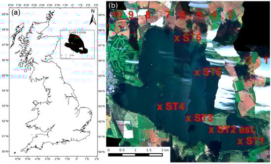
Figure 1.
(a) map showing the location of Loch Leven within the UK; (b) Image mosaic from 10 FENIX flight lines collected during the campaign (colours are illustrative only). Locations of the in situ station measurements are marked with red crosses; the location of station ST2 is approximate.
2.2. Remote Sensing Data
2.2.1. Airborne Data Collection
Airborne hyperspectral data were acquired on 7 August 2014 between 11:20 and 12:27 (local time) with an AisaFENIX sensor (Specim, Spectral Imaging Ltd, http://www.specim.fi/) on board a NERC Airborne Research Facility (National Environment Research Council Airborne Research Facility http://www.bas.ac.uk/nerc-arf) aircraft. In total, 10 flight lines were flown from south to north (Figure 1, Table 1). The flying height was approximately 1500 m, resulting in a ground sampling distance of 2 m. The campaign was carried out in challenging illumination conditions, as clouds and cloud shadows were clearly visible on several FENIX images (Figure 1). The FENIX data used for this publication are available to download from the NERC Earth Observation Data Centre (NEODC; http://neodc.nerc.ac.uk/).

Table 1.
Flight lines, in situ reference measurements and atmospheric parameters during the campaign. FL2-9: flight line number, ST1-6: in situ measurement station number. Times are local time (BST). Wind: average wind speed during station measurements. QC pass/All: number of individual spectrum that passed the automatic quality control during station measurements. In situ water vapour and AOT values used for atmospheric correction strategy AC3 are given in italics. wv: columnar water vapour, AOT: aerosol optical thickness, Vis: horizontal visibility, A.: parameter derived by ATCOR (wv and AOT with standard deviations, MT: Microtops sun photometer used for in situ AOT and water vapour measurements.
FENIX is a pushbroom sensor with a wavelength range 380–2500 nm and 384 spatial pixels. FENIX has two separate physical detectors to record the whole wavelength range: a CMOS (Complementary Metal Oxide Semiconductor) detector for the VNIR range (380–970 nm) and an MCT (Mercury Cadmium Telluride) detector for the SWIR range (970–2500 nm). The sensor was operated in spectral binning mode, resulting in 448 bands (174 bands in VNIR, 4x binning; 274 bands in SWIR, no binning) with average spectral sampling interval 3.4 nm on VNIR range and 5.7 nm on SWIR range. The spectral resolution is 3.5 nm on VNIR and 12 nm in SWIR range. The peak signal-to-noise ratio (SNR) of the sensor is 500–1000.
Sensor radiometric calibration data from laboratory measurements were applied to the images at NERC-ARF-DAN (NERC Airborne Research Facility—Data Analysis Node, https://nerc-arf-dan.pml.ac.uk) to convert the raw image data to at-sensor radiance data in the original sensor geometry [42].
2.2.2. SNR Estimation
To estimate the FENIX signal-to-noise ratio, at-sensor radiance image data were used and 31 regions of interest (ROI) containing 100 pixels over water (10 × 10 pixels, approximately 20 × 20 m) were defined from 7 flight lines. The location of each ROI was manually selected over the most uniform areas of the water body so that the standard deviation of the ROI radiance would be a close representation of sensor noise. The measured mean at-sensor radiance of each ROI was divided by the standard deviation of the ROI to calculate per-band SNR = mean/stdev [43]. ROIs where the standard deviation was lowest (<0.0002 (W/m2/sr/nm)) and uniform between 450 and 900 nm were considered least affected by in-water variability of optically active constituents, and selected for final SNR calculations. The final estimate of sensor SNR was then calculated as the per-band average of the 17 best quality ROI SNR measurements. This image-based SNR evaluation takes into account the whole sensor–atmosphere–target system and gives estimation of the sensor SNR in real operational conditions.
2.2.3. Atmospheric Correction with ATCOR4
ATCOR4 version 7.0.0 [28], which is based on the radiative transfer model MODTRAN5 [44], was used for the atmospheric correction of the hyperspectral data. ATCOR4 is highly configurable, and includes a number of built-in algorithms to automatically select a number of input parameters, including water vapour, horizontal visibility and aerosol model, from the imagery supplied. These algorithms require narrow bands in the VNIR-SWIR range. If the sensor does not have the required bands and/or there are in situ atmospheric data available, these parameters can also be set manually. The aim of the current analysis was to validate the use of the built-in algorithms for operational processing environments, rather than optimize each input parameter manually and separately for each image.
The following ATCOR4 parameters for the first atmospheric correction (AC1) were used with all flight lines: aerosol model: rural (detected by ATCOR4), spatially variable water vapour (detected by ATCOR4), variable horizontal visibility (detected by ATCOR4). AOT (aerosol optical thickness) over water was set to be interpolated from land values. Water vapour detection was based on bands in the 940 nm and 1130 nm regions. The mean AOT and water vapour values for each flight line, with standard deviation values illustrating the variability of the parameter, are shown in Table 1. The end result of the atmospheric correction was a set of reflectance images with normalized water-leaving reflectance Rw(λ) (dimensionless, range [0, 1]) [45] values for each image pixel and band. If the correction would result in negative reflectance values, ATCOR4 will convert them to a constant reflectance value of 0.0025.
Two other built-in ATCOR4 atmospheric correction strategies were also tested with flight lines FL4 and FL5. In the second strategy (named AC2), horizontal visibility and water vapour were detected by ATCOR4, but all of were fixed for the whole image. In the third strategy (AC3), parameters were set to be fixed for the whole image based on in situ measurements (Table 1). Otherwise, all options were kept the same as in AC1. In situ AOT values were converted to horizontal visibility using the Koschmieder equation [28]. The ATCOR4-recommended horizontal visibility values for AC2 was 100 km for both flight lines, FL4 and FL5. The fixed water vapour values in ATCOR4 can only be set by choosing from predefined values, so the closest value in the list, 1.0 cm, was used for all strategies. Both strategies, AC1 and AC2, are fully image driven.
2.3. In Situ Reflectance Measurements
A boat-based sampling campaign was carried out simultaneously with the airborne campaign, between 10:53 and 15:59 BST, to measure remote sensing reflectance Rrs [45] with a system based on three TriOS RAMSES spectrometers (http://www.trios.de/). The system recorded spectral water-leaving radiance Lw(λ) and sky-radiance Lsky(λ), as well as downwelling irradiance Ed(λ) in the λ = 320–950.3 nm wavelength range in 192 channels. With a 3.3 nm sampling interval. Six sampling locations (ST1-6, Figure 1) were visited, where the boat was kept stationary and Rrs data were recorded for 5–10 min resulting in 30 individual spectra (Table 1). Also, AOT measurements with a Microtops II sunphotometer were performed during the sampling campaign (Table 1, Figure 2).
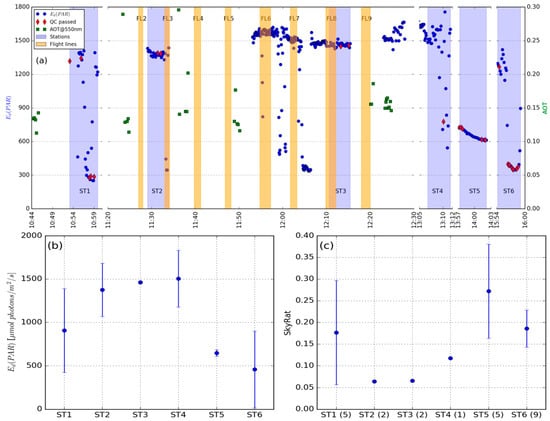
Figure 2.
(a) In situ Ed(PAR) and AOT measurements taken during the campaign. In situ observations used for station reference spectra are marked with red diamonds. Orange shading indicates the times of airborne flight lines, and blue shading the times of station measurements; (b) Median and standard deviation of Ed(PAR) from all 30 measurements recorded at each station; (c) SkyRat based on QC passed measurements for calculation of Rrs (number of valid observations are shown in horizontal axis label). The SkyRat error bars for stations ST2-ST4 are not shown, as there were <3 valid measurements at these stations.
The target for viewing geometry of the in situ radiance measurements from the boat was for a 40 degrees oblique angle from zenith and 135 degrees from solar azimuth, corresponding to a minimum of sun-glint [45] and avoiding shadows and reflections from the sampling platform. Prevailing weather conditions, with wind speeds 1.4–6.2 m/s, and use of a small boat will have caused occasional deviations from these optimal angles. While cruising between stations and simultaneously recording transect measurements, the GPS heading is sufficiently accurate to derive the azimuth angle of the sensors, and measurements with inappropriate viewing geometry were thus removed from the data set. While cruising between stations ST1 and ST3, GPS information was not recorded, so for these station ST2 the location was estimated by spatiotemporal interpolation between start and destination locations. The station locations are marked in Figure 1, with uncertain location information marked separately.
Post-processing of the radiance data to calculate Rrs (units sr−1) followed the protocol of Simis and Olsson [46], which also flags suspect measurements. Only Rrs spectra that passed the quality control procedure were used (QC passed). Median and standard deviation Rrs spectra were calculated for each station where at least two valid Rrs spectra were thus obtained. The median Rrs spectrum of each station was used as reference for the airborne observations.
Two additional indicators of illumination conditions during the in situ Rrs measurements were calculated during post processing. First, Ed integrated over the spectrum of photosynthetically active radiation (Ed(PAR), 400–700 nm), is used to express the intensity of solar irradiance during a measurement. Second, the ratio πLsky(400)/Ed(400) (SkyRat) is indicative of the cloudiness during a measurement. SkyRat < 0.2 are generally indicative of clear sky conditions, whereas values close to unity suggest overcast conditions [46].
Weather Conditions
Weather conditions, in particular cloud cover, varied significantly during the campaign. In situ above-water Rrs can be measured under clear, fully overcast, and sometimes even under partially clouded conditions. In general, there is a larger margin for error in relatively turbid waters where water-leaving radiance is high compared to skylight reflected on the water surface. Variable illumination conditions (high standard deviation of SkyRat and Ed(PAR)) are least favourable, because the measured spectrum of sky radiance is less likely to represent the sky radiance reflected on the water surface. Figure 2 shows the variations of in situ-measured Ed(PAR) and AOT during the campaign, with shading indicating the timing of airborne observations and in situ station measurements. As an indication of illumination conditions during in situ Rrs station measurements, SkyRat and Ed(PAR) values, with standard deviation error bars for each station, are shown in Figure 2. Ed(PAR) values are based on all 30 observations performed during each station measurement, whereas SkyRat values are based only on spectra for which Rrs could be derived, as these are obtained using suitable viewing geometry for the radiance measurements. Stations ST2 and ST3 had the lowest SkyRat values and highest Ed(PAR) radiances, indicating clear sky; still, only two individual spectra passed the quality control for these stations. When stations had more QC-passed measurements (ST1, ST5, ST6), also the standard deviations of these measurements increased. From the Ed(PAR) values in Figure 2 (top) and SkyRat values in Figure 2 (bottom right), it can be seen that illumination conditions varied highly during stations ST1 and ST4, were relatively stable and good during stations ST2 and ST3, were stable and cloudy during station ST5 and were variable but mainly cloudy during station ST6. The measured in situ AOT values varied between 0.12 and 0.3 during the flight campaign. As the weather got cloudier during and after station ST4 measurements, it was not possible to acquire additional in situ AOT measurements.
2.4. Data Analysis
To allow quantitative comparison of image and in situ spectra, in situ Rrs spectra were converted to normalized water-leaving reflectance Rw (where Rw = π × Rrs). This assumes that the upwelling radiance is fully diffuse, whereas its angularity is not strictly known. Subsequently, in situ Rw spectra were interpolated to match the FENIX wavelength grid in the range between 383 nm and 948 nm, where the two sensor systems overlap. To reduce the effect of sensor noise, image Rw data were spatially averaged over 3 × 3 pixels, approximately 6 × 6 m, to obtain the final image spectrum for each station. When comparing exclusively the spectral shapes of in situ and airborne Rw, both were standardized between their minimum and maximum values to the range [0, 1].
The dataset allowed ten comparisons between ATCOR4-derived and in situ Rw spectra. There were seven spatial matches between images and in situ station measurements. Due to the image overlap between adjacent flight lines, station ST3 was visible on both flight lines FL5 and FL6. Three additional comparisons were done between stations ST1, ST4 and ST6 and nearly matching flight lines FL3 (45 m distance), FL8 (72 m distance) and FL7 (90 m distance), respectively. The time difference between flight lines and in situ station measurements varied from 9 min to four hours; station ST1 was measured before the airborne observations started, stations ST2 and ST3 during the campaign and stations ST4-6 following the airborne observations. Table 1 and Table 2 give the details of the comparisons and their spatial and temporal differences.
Table 2.
Chi-squared (X2) and spectral angle (SA) metrics and Chl-a retrieval difference for all 10 matchups between in situ and image Rw. T.diff: time difference between in situ measurement and aircraft overpass; negative time means that in situ measurement is done before, and positive after, the airborne measurement. Dist.dif: distance between in situ and image measurement locations. Full: full wavelength range 383–948 nm, cen: centre part of the spectra 450–750 nm. Chl-a diff: Chl-a concentration difference between image and in situ-based retrieval in (mg/m3). Range for the SA is [0, 180]. In both metrics, values closer to 0 indicate more similar spectra. Results from five best matchups are in bold. Measurement location on FL6 was covered with cloud shadow (results in italics). X2 and Chl-a diff values for comparison ST5-FL5 full were not relevant as the in situ spectra had negative values above 750 nm, which are not allowed in the calculation of the metric.
Differences between in situ and image Rw spectra were compared using the following numerical evaluations: evaluation of spectral accuracy by using spectral difference, spectral ratio and root mean square difference (RMS), and calculation of Spectral Angle (SA) [47,48] and Chi-square (Χ2) metrics to evaluate the similarities in spectral shapes.
Analysis of the reflectance accuracy followed the method described in Markelin et al. [49]. In short, reflectance accuracy was evaluated by first considering the absolute difference (ΔRw) between measured Rw (Rw_data) and the in situ Rw (Rw_ref). This difference was then expressed as the relative difference (ΔRw% = 100% ΔRw/Rw_ref). ΔRw and ΔRw% were calculated for all comparisons in the matching wavelength range of 383–948 nm. From these differences, root mean square difference values (RMS and RMS%) were calculated using all 10 comparisons and 5 qualitatively best ones as follows:
where n is the number of observations. RMS is calculated using Equation (1) by replacing ΔRw% with ΔRw.
The spectral angle is a metric comparing spectral shapes, insensitive to spectral amplitude, and is calculated as:
where a denotes ATCOR4-derived spectra, t are in situ spectra and nb is the number of channels/bands in a spectrum. In practice, the spectral angle is the angle between two vectors (spectra) and is not sensitive to differences in amplitude that are consistent over the whole spectrum. The range for the spectral angle is [0, 180] (or 0–π radians), where values close to 0 indicate high similarity.
Chi-square takes both the shape and the amplitude of the spectra into account, where the sum of all bands is considered for each spectrum, and is calculated as:
where a and t are as in (2) and nb is the number of channels/bands in a spectrum.
Additionally, visual comparison of in situ and image Rw spectrum plots was also performed to address specific anomalies, such as areas in the spectrum with consistent error patterns or high noise, the reproduction of key spectral features and to evaluate the homogeneity of the lake.
2.5. Chlorophyll-a Retrieval
To evaluate the applicability of the atmospherically corrected imagery in water quality monitoring, we selected semi-analytical band ratio algorithm suitable for turbid inland waters to retrieve Chl-a concentrations from in situ and image Rw spectra. The algorithm presented by Gons et al. [50] was designed for MERIS, and widely used for coastal and inland waters with Chl-a concentrations >10 mg/m3, such as Loch Leven [26]. First, the backscattering coefficient bb is calculated as:
where Rw(778) is water-leaving reflectance of the MERIS equivalent band 12 centered at 778 nm. Then, the Chl-a concentration is calculated as:
where Rw(708) and Rw(665) are water-leaving reflectance for MERIS bands 9 and 6, centered at 708 nm and 665 nm, respectively. As MERIS bands 6 and 9 are 10 nm wide and band 12 is 15 nm wide, the average of three FENIX 3.3 nm wide and TriOS 3.5 nm wide bands were used in calculations. Equation (5) was used to calculate Chl-a concentration in (mg/m3) from both image-derived and in situ Rw spectra. Image- and in situ reflectance-based concentrations were compared by calculating Chl-a differences and RMS both in mg/m3 and in percent using Equation (1).
3. Results
3.1. Variability in Water-Leaving Reflectance
From 50 randomly selected Rw spectra representing the whole lake (Figure 3a), it becomes evident that the amplitude of the spectra varies significantly more than their shape. The water is therefore understood to be relatively homogenous in terms of the relative composition of optically active substances. Spectral features caused by chlorophyll-a are clearly visible from a reflectance trough near the red absorption peak of the pigment at 650 and 700 nm. The amplitude of spectra is low but non-zero at wavelengths above 950 nm, where the absorption by pure water dominates the optical properties of the water.
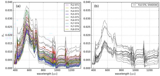
Figure 3.
(a) Rw spectra measured from atmospherically corrected FENIX images. Spectra measured at station locations are shown in colour, grey spectra are an additional 50 measurements representing all lake areas to indicate the homogeneity of the lake; (b) Image-based Rw spectra of water measured from 21 locations under cloud shadows, the black line indicates station ST6 on image FL6. Wavelength range in the x-axis goes up to 1300 nm to indicate the non-zero reflectance in the NIR-SWIR range.
Atmospheric absorption caused by water vapour is seen in at 820, 940 and 1130 nm wavelength regions, where the shape of the spectra is disturbed and the atmospheric correction cannot succeed. Several spectral features likely resulting from suboptimal sensor calibration are also visible in the Rw spectra. The sharp peak visible at 425 nm cannot be associated with in-water optically active substances. Numerous narrow variations in spectral shape, e.g., between 560 and 700 nm, are either sensor or atmospheric correction issues, since water constituents do not show sharply featured optical features in the visible domain (see in situ reference spectra, Figure 4). Rw values of 0.0025 in the area around 400 nm suggest that negative reflectance values resulted from ATCOR4 processing, which ATCOR4 then converted to this low constant value.
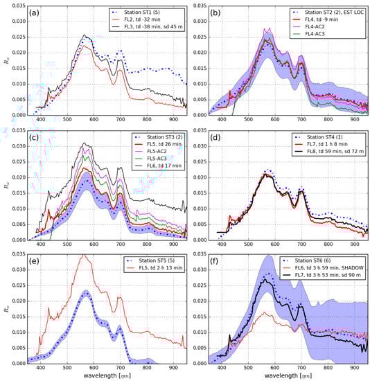
Figure 4.
(a–f) In situ station and image-derived Rw of each matchup. The best matchups in terms of Chi-square and spectral angle are shown in a thicker line in panels (b–d,f); Image Rw from atmospheric correction strategies AC2 and AC3 are included in panels (b,c); Bracketed values in the panel legends state the number of spectra used to calculate the in situ spectrum and error bars; td = time difference between in situ measurement and image acquisition, sd = distance between in situ and image matchup measurement, if applicable. Standard deviations for the in situ station measurements are plotted as error bars (blue shading) where available.
An additional 20 spectra were sampled from the images in areas shadowed by clouds (Figure 3b). Here, the Rw spectra were dampened in the 400–750 nm range, but maintained the spectral shape of Rw measured at clear sky locations, suggesting that the interpretation of Rw by ATCOR4 is primarily hampered by an unknown intensity of downwelling irradiance in these shaded areas. At wavelengths beyond 750 nm the signal was comparable to non-shaded locations.
3.2. Evaluation of AisaFENIX SNR
Image-based per-band SNR estimation for FENIX, calculated as the mean of image Rw from 17 locations over water, is shown in Figure 5. Because the SNR is dependent on the radiance recorded at the sensor, the mean at-sensor radiance at these locations is also included. The SNR is approximately proportional to the amplitude of at-sensor radiance, as expected. The edges of linear arrays of the FENIX CMOS (380–410 nm and 960–980 nm) and MCT detectors (960–980 nm) show lower SNR, which is a detector property. The maximum measured SNR ranged from 40–95 in the 450–750 nm wavelength range. Over bright clouds, SNR ranged from 400–550 in the 500–800 nm wavelength range, and approximately 30 elsewhere.
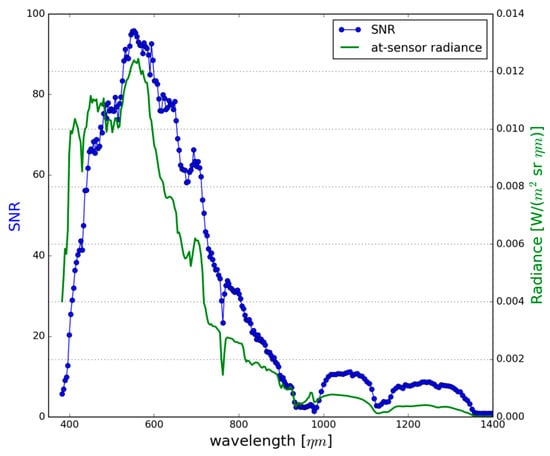
Figure 5.
Spectral signal-to-noise ratio (SNR) (blue circles) and at-sensor radiance (green line) of AisaFENIX measured over Loch Leven. Curves are mean of 17 individual measurements from 7 flight lines.
3.3. Effect of Atmospheric Parameters in ATCOR4
Three different atmospheric correction strategies in ATCOR4 were tested to find one suitable for operational use. The image-derived Rw from each strategy used for flight lines FL4 and FL5 are shown in Figure 4b,c. The most accurate results compared to in situ Rw were achieved with strategy AC1, where both water vapour and horizontal visibility were detected by ATCOR4 and those parameters were allowed to vary spatially. When using fixed water vapour and visibility values for whole images (AC2 and AC3), there was a small amplitude difference between image and in situ Rw. The spectral shapes of Rw from AC2 and AC3 were practically identical (Figure 6b,c), meaning that the change in the input visibility caused a fixed shift in amplitude in Rw. As there were only small differences between the three strategies tested, and the primary aim of our work is to derive an operational atmospheric correction approach without dependence on in situ data, the rest of the analysis was performed for image Rw based on atmospheric correction strategy AC1.
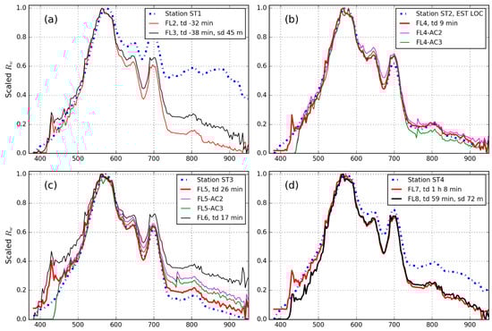
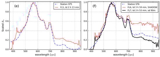
Figure 6.
(a–f) In situ station and image-derived Rw spectra standardized between 0 and 1. Image spectra corresponding to the best five comparisons are plotted as thicker lines. Image-derived standardized Rw from atmospheric correction strategies AC2 and AC3 are included in panels (b,c). In panel legends, td = time difference between in situ measurement and image acquisition, and sd = distance between in situ and image measurement.
3.4. Station-Wise Comparisons of Rw
The campaign resulted in seven spatially matching pairs of airborne and in situ observations. Due to image overlap between adjacent flight lines, station ST3 was visible on flight lines FL5 and FL6. Additionally, three matchups were included from approximately matched station locations (ST1-FL3 at a distance of 45 m, ST4-FL8 at a distance of 72 m and ST6-FL7 at a distance of 90 m). The ten matchups are listed in Table 2. If a station included more than one successful in situ reflectance spectrum, these were used to calculate standard deviation error bars around the median spectrum for that station (Figure 4). Error bars are omitted for station ST1 due to extremely varying illumination conditions. The location of station ST6 on image FL6 was under cloud shadow, but the matchup spectra are included for comparison.
Based on both quantitative (Table 2, Figure 7) and qualitative (Figure 4 and Figure 6) analysis, the best results were obtained for the comparison between station ST2 and image FL4. There, the image and in situ spectrums matched closely over the wavelength range 380–950 nm and the image-derived spectrum was always within the standard deviation of the in situ observations. Other good matches were ST3-FL5, ST4-FL7, ST4-FL8 and ST6-FL7. At these matchups, the spectral shape of image-derived Rw matched well with the in situ spectra, and the difference in amplitude was less than 0.005 in reflectance units. Still, the image-derived Rw included some errors common to all images, most notably the spike at 425 nm. In the other matchups, typical differences between image and in situ spectrums were either a clear difference in amplitude (as in matchups ST3-FL6, ST5-FL5), or shape difference in some part of the spectra (as in matchups ST1-FL2, ST1-FL3, ST6-FL6). The spatial difference between in situ and image measurements did not seem to have any notable effect on the matchups: ST4-FL8 and ST6-FL7, with spatial differences of 72 m and 90 m, respectively, gave good results comparable to matchups with no spatial difference. There was no notable effect of temporal differences between matchups. The time differences for the best five matchups were between −0:09 and 3:59, and between −0:38 and 3:53 for the worst five matchups.
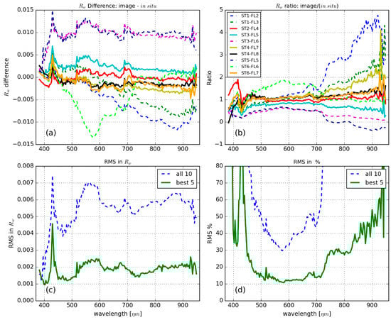
Figure 7.
(a) Difference between image-derived and in situ Rw; (b) ratio of in situ over image-derived Rw; (c) RMS of the best five and all matchups, respectively, in units of reflectance; (d) Relative RMS. Matchup labels for panes (a,b) are given in the legend of panel (b), and the five best matchups are plotted with a solid line.
Table 2 lists results from Chi-squared and spectral angle metrics used to evaluate spectral differences between in situ and image Rw spectra. Metrics are shown for both the full wavelength range (383–948 nm) and the centre of the spectra (450–750 nm). Both metrics gave similar results in ranking the matchups from best to worst. The best five matchups (ST2-FL4, ST3-FL5, ST4-FL7, ST4-FL8, ST6-FL7) remained the same regardless of using either the full wavelength range or using only the centre part of the spectra. Using only the centre part of the spectra clearly improved the results on both metrics, as both the image and in situ spectrums suffer from low signal in the wavelengths below 450 nm and above 750 nm. The spectral angle gave values of 4.06° or better, and 3.00° on average, for the five best matchups, and 10.4° or better, with 8.85° on average, for the worst five matchups, when considering the centre of the spectra. Chi-square metrics were 0.068 or better, and 0.024 on average, for the five best comparisons, and 5.3 or better, or 1.35 on average, for the remaining five comparisons, when using the centre part of the spectra.
Both the Chi-squared and spectral angle metrics were worse for atmospheric correction strategies AC2 and AC3 than for AC1 for flight lines FL4 and FL5-ST3. The spectral angle gave values of 10.4° and 13.2° for FL4-AC2 and FL4-AC3, and 8.7° and 7.2° for FL5-AC2 and FL5-AC3, respectively, when using the full wavelength range. The respective values when using the centre part of the spectra were 4.2° and 6.0° for FL4-AC2 and AC3, and 3.7° and 2.9° for FL5-AC2 and AC3. Chi-squared values were 0.51 and 0.023 for FL4-AC2 and FL4-AC3, respectively, and 0.401 and 0.204 for FL5-AC2 and FL5-AC3, respectively, when using only the centre part of the spectra.
The RMS and relative RMS difference between in situ and image Rw were calculated for all 10 matchups and for the best five matchups separately, using both Chi-square and spectral angle metrics, with the centre of each spectrum taken into account (Figure 7). The spectral difference plot of image and in situ Rw (Figure 7a), and RMS in Rw (Figure 7c) show that the difference remained relatively stable over the whole wavelength range. This is also visible in the spectral plots of Figure 4. The spectral ratio of image and in situ Rw (Figure 7b) and RMS% plots (Figure 7d) show that, as the water-leaving reflectance signal becomes weaker at wavelengths longer than 700 nm, the uncertainty or error in matchups becomes larger. This effect is also visible in the standardized Rw matchup plots in Figure 6. The best five matchups in terms of RMS had ±0.002 accuracy in reflectance, or better than 15% in terms of RMS%, in the 450–750 nm wavelength range.
Matchup ST6-FL6 was disturbed by cloud shadow in image, and the magnitude of image-derived Rw deviated strongly from in situ Rw in the 450–750 nm wavelength range (Figure 4). When considering only spectral shape in the 450–750 nm wavelength range, the spectral angle value was 7.7°, comparable to other matchups. This is illustrated in the standardized spectra plotted in Figure 6f.
3.5. Comparison in Terms of Retrieved Chlorophyll-a
Chl-a concentrations were calculated from all measured image Rw spectra (Figure 8a), including locations under cloud shadow, and from all in situ station spectra, except ST5, as it included negative reflectance values. Chl-a concentration derived from in situ station spectra varied between 17.8 to 30.9 mg/m3 and was, on average, 24.9 mg/m3. Concentrations derived from the image spectra varied between 19.9–43.1 mg/m3, with an average of 28.7 mg/m3 and standard deviation of 3.8 mg/m3. When looking only at the station data, concentrations varied between 25.9 and 35.3 mg/m3 and the average was 31.0 mg/m3. Measurements located under cloud shadows produced concentrations between 19.8 and 52.9 mg/m3, with an average of 30.3 mg/m3 and standard deviation of 7.2 mg/m3.
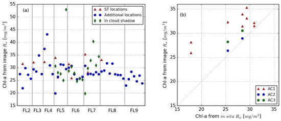
Figure 8.
(a) Chl-a values in (mg/m3) derived from all measured image Rw; (b) scatter plot between Chl-a values derived from in situ Rw and image Rw at station locations.
A scatter plot comparing in situ and image-derived Chl-a concentrations is given in Figure 8b, including Chl-a derived from images using atmospheric correction strategies AC2 and AC3. The Chl-a difference values between nine matchups with AC1 are shown in Table 2. It can be seen from Figure 8b that image-derived Chl-a concentrations were consistently higher than concentrations derived from in situ Rw. Also, apart from Chl-a values from ST6 (17.8 mg/m3), the concentrations are all of the same order, indicating that the water type of Loch Leven is relatively homogenous. The RMS and relative RMS% difference between in situ and image-derived Chl-a concentrations were 5.87 mg/m3 and 28.3%, respectively, when using all nine matchups. When leaving out the matchups with ST6 that was measured during the most challenging illumination conditions, the RMS and relative RMS% improved to 4.4 mg/m3 and 16.1%, respectively.
4. Discussion
4.1. Reflectance Quality of the Best Case Results
AisaFENIX Rw spectra obtained after ATCOR4 atmospheric correction were realistic for Loch Leven and showed good correspondence with concurrent in situ Rw, both in terms of spectral shape and magnitude. Different atmospheric correction strategies produced differences, especially in the amplitude of the image Rw. The best reflectance accuracy was achieved with the strategy using image-driven retrieval of spatially varying water vapour and horizontal visibility (and subsequently AOT). Five matchups between atmospherically corrected image and in situ Rw data were in excellent agreement in the wavelength range 450–750 nm, preserving features associated with Chl-a absorption. Taking into account only the spectral shape, the Spectral Angle metrics were better than 4.1° for the best five matchups. For comparison, spectral angles between 5.7° and 28.6° (0.1–0.5 rad) have been used as thresholds in Spectral Angle Mapper (SAM) classification, comparing image-derived Rw to reference Rw [51,52]. Errors in water constituent retrieval (e.g., Chl-a) would thus more likely be associated with the presence of systematic errors resulting in an offset of the image-derived spectra than with the correct retrieval of the spectral shape.
The accuracy of ATCOR over inland water bodies using in situ reflectance spectra has not previously been evaluated in literature. In general, the authors of ATCOR4 software estimate that accuracy of retrieved surface reflectance of ±2% for object reflectance <10% can be achieved [53]. Markelin et al. [34] achieved reflectance accuracy better than 10% when using ATCOR4 to correct hyperspectral AisaEAGLE data over land targets. Hunter et al. [26] used FLAASH atmospheric correction with AisaEAGLE imagery collected over Loch Leven and achieved a RMS% range from 26.4% to 77.7% in the 400–800 nm wavelength range, compared to in situ Rrs. Compared to these results, and taking into account the challenging illumination conditions during the campaign, the reflectance accuracy of better than 15% achieved here can be considered a very promising result.
Acquiring the aerosol properties and their distribution over the campaign area, either by in situ measurements or by image-based algorithms, is crucial for accurate atmospheric correction [20,30]. Differences of 0.01–0.07 between scene-averaged AOT given by ATCOR4 and in situ sunphotometer AOT measurements are in line with results obtained by Pflug et al. [54]. Using satellite imagery, they evaluated the accuracy of the aerosol retrieval in ATCOR and found the mean uncertainty ΔAOT550 nm to be 0.03 ± 0.02 for cloud-free conditions and ΔAOT550 nm 0.04 ± 0.03 with inclusion of hazy and cloudy satellite imagery, compared to ground-based sun photometer measurements.
The image-based method used in this study to estimate sensor signal-to-noise ratio gives SNR representative for the whole sensor–atmosphere–dark target system. These values cannot be directly compared to the laboratory-measured SNR values from the sensor manufacturer. The SNR range of 450–800 determined over bright cloud in this study is nevertheless comparable to the laboratory peak SNR of 500–1000 documented by Specim. Measured over water, with average reflectance in the order of 0.02, the FENIX SNR range of 40–95 is similar to the range of 60–120 for the older AisaEAGLE sensor reported by Markelin et al. [34], which was, however, measured over a much brighter target, with average reflectance of 0.26. This indicates that the SNR of FENIX has improved considerably over its predecessor.
4.2. Chlorophyll a Retrieval
The retrieved Chl-a concentration range of 25–35 mg/m3 is well within the range documented for Loch Leven [26,40]. Concentrations derived from the imagery overestimated Chl-a with respect to in situ Rw. Interestingly, the Chl-a concentrations derived from images corrected with AC2 and AC3 matched similarly or better with in situ Rw, compared to AC1 (Figure 8), even though the spectral match based on Chi-Square and spectral angle metrics was better with AC1. These contrasting results are not well understood and without further validation against Chl-a extracted from water samples we should not consider Chl-a derived from in situ Rw an absolute reference. Although speculative, minor spectral features that are still visible in FENIX-derived spectra and which coincide with wavebands used in the Chl-a retrieval algorithm, such as a small depression in the 700-nm region, may well disturb the results from the NIR-red band ratio algorithm. In addition, variable and at times adverse weather conditions will have added uncertainty to in situ measurements (see Section 4.3). Still, the achieved RMS of 5.87 mg/m3 and RMS% 28.3% are well in line with Hunter et al. [26]. They evaluated several empirical and semi-analytical algorithms, including the one used in this study, to retrieve Chl-a from hyperspectral AisaEAGLE and CASI imagery collected over Loch Leven and Esthwaite Water, and obtained RMS values from 5.29 to 22.1 mg/m3 and RMS% from 29.8 to 124%, respectively. Moses et al. [24] obtained similar RMS of 5.54 mg/m3 when also using semi-analytical three-band Chl-a retrieval algorithm for AisaEAGLE imagery in combination with QUAC atmospheric correction. The Gons et al. [50] semi-analytical NIR-red band ratio algorithm is generally forgiving to spectrally neutral offsets, as long as none of the wavebands used are near-zero. Indeed, Chl-a retrieval from image Rw at locations under cloud shadow gave concentrations comparable to non-shaded locations.
4.3. Uncertainties Related to FENIX, In Situ Rw and Atmospheric Correction
Even though the results achieved in this study are promising, several factors related to the sensor, in situ measurements and atmospheric correction contribute uncertainty to the results. First, SNR values are extremely important for water constituent retrieval, because the very low signal from water causes variations in water quality to be lost in the noise of low SNR systems. The SNR of the AisaFENIX sensor over water is still low compared to dedicated ocean colour satellite instruments such as Sentinel-3 OLCI (SNR 200-1000). The image-based SNR evaluation method is somewhat uncertain in the sense that the standard deviation of each ROI includes small (unknown) contributions from variability in water-leaving radiance. Further, the combination of lower SNR of the FENIX and low signal from the water at wavelengths >750 nm makes comparison of airborne and in situ Rw in these regions challenging.
Low but non-zero image Rw in the order of 0.005, at wavelengths above 1000 nm, can indicate inaccuracies/uncertainties of atmospheric correction, as Rw is expected to be zero even in relatively turbid lakes, due to high absorption by pure water. Natural causes for non-zero Rw in this wavelength region include floating matter, very high turbidity [35], adjacency effects from the land surface, spray, foam (whitecaps), entrained bubbles or thin cloud. Prevailing weather conditions during the campaign, with wind speeds 1.4–6.2 m/s, raises the likelihood of wave effects, which adds uncertainty to both in situ and image Rw spectra.
The differences in the amplitude of the observed Rw spectra can be related to both the inaccuracies of the atmospheric correction and some variations in the relative composition of optically active substances in the water. Different atmospheric correction strategies did result in spectra of different amplitudes (Figure 4b,c) and adherent changes in Chl-a retrieval. One limitation of the used ATCOR4 atmospheric correction method applied to water objects is that it uses the Dark Dense Vegetation (DDV) approach to estimate best horizontal visibility, and subsequently AOT, for an image [28]. Each image must thus include suitable vegetated areas.
In this study, full-width-half-maximum (FWHM) values and centre wavelength for each channel, read from the image headers, and Gaussian spectral shapes, were used to create the FENIX spectral response functions in ATCOR4. This sensor model was then used in ATCOR4 processing. Sensor radiometric laboratory calibration performed by the manufacturer in January 2016 indicated that the used FWHM values may deviate, on average, 0.16 nm from the true FWHM in the visible-NIR range. Even though the error in FWHM can be considered marginal, it may explain some small spectral variation and spikes in the Rw spectra. Two narrow spikes around 700 nm where there should only be a single smooth peak, and a peak around 425 nm, likely result from a sensor calibration or software issue. Indeed, the peak disappeared from newer ATCOR4 runs (AC2 and AC3) performed with an updated sensor model and ATCOR4 version. Unfortunately, it was not possible to rerun all performed ATCOR runs. Thompson et al. [55] concluded that uncertainty in solar irradiance is a likely contributor to fine-scale spectral errors in Rw, especially in the 380–600 nm spectral range. Spectral filtering or polishing, a common operation performed with hyperspectral imagery, could be used to remove these small-scale variations in spectral shape and further improve results [56], if this were shown to consistently improve retrieval accuracy.
The varying weather conditions added considerable uncertainty to in situ Rw spectra. This can be seen in the low number of spectra that passed QC during measurements at several stations (Table 1) and the wide standard deviation of these spectra (Figure 4). The Ed(PAR) and ratio of diffuse sky radiance in Figure 2 show that the illumination conditions were highly variable. Negative reflectance values (not a true target property) of in situ ST5 Rw spectra at wavelengths over 750 nm are a clear indication of these challenging conditions, despite Ed(PAR) being relatively stable at this station. Similarly, the ST1 in situ spectrum (Figure 4a) shows particular signs of disturbance (possibly by waves, ship roll, or glint) in the NIR.
The number of matchup locations is always limited in this type of study, and prevents more thorough analysis of between-image reflectance variations. For example, ATCOR4 offers a sophisticated method called BREFCOR to balance the reflectance differences between neighbouring images [28], which could be included in future studies but ideally requires more ground reference measurements. Relatedly, flight lines and in situ measurements were obtained at different times, varying from 9 min to 4 h difference. Variable winds may cause horizontal differences in sediment and detrital resuspension, although in this study, temporal differences between matchups were not identified.
5. Conclusions
We presented the first results of using the hyperspectral AisaFENIX airborne sensor in water quality applications. The imagery was collected over a small inland water body under changing cloud cover, illustrating highly challenging, but not uncommon, conditions for atmospheric correction. The FENIX sensor showed improved performance in terms of signal-to-noise ratio compared to its predecessor, AisaEAGLE. Atmospheric correction performed with ATCOR4 using fully image-driven atmospheric parameters, and subsequent validation against boat-based in situ hyperspectral measurements of water-leaving reflectance, show reflectance retrieval accuracy of ±0.002, i.e., better than 15% error for the best five matchups between image and in situ Rw spectra. The reflectance accuracy was better when using fully image-driven atmospheric parameters compared to using fixed parameters based on in situ measurements. The spectral angle between image and in situ Rw spectra was better than 4.1° for the best cases and 10° or better for the most challenging cases in the spectral range of 450–750 nm. The test with semi-analytical band ratio-based algorithm to retrieve Chl-a concentrations from image Rw spectra gave realistic concentrations and the accuracy was comparable to other studies. The results showed that ATCOR4 can be successfully used for water applications without in situ atmospheric measurements, even in challenging illumination conditions. As ATCOR4 does not a priori assume a water reflectance, it is expected that the presented atmospheric correction method can be applied for images collected over other relatively turbid inland water types as well. The results also indicate that, with accurate atmospheric correction, it could be possible to retrieve reliable Chl-a concentrations at locations covered by cloud shadow. Accurate atmospheric correction is a necessity when airborne (manned or unmanned) optical measurements are performed in challenging illumination conditions, even under cloud cover. We may expect that future airborne monitoring of inland waters will build on advances in unmanned aerial system (UAS) technology and high resolution satellite sensors.
Acknowledgments
Airborne data were acquired by the Natural Environment Research Council Airborne Research Facility (NERC-ARF) as part of project GB12/03. UK Natural Environment Research Council (NERC) GloboLakes projects (Grant Number: NE/J024279/1 www.globolakes.ac.uk) supported the efforts of P. Hunter, V. Spyrakos, A.N. Tyler and S. Simis.
Author Contributions
Lauri Markelin wrote the manuscript with contributions from all authors. Lauri Markelin performed atmospheric correction and data analysis; Lauri Markelin, Stefan G. H. Simis and Steve Groom conceived and designed the analysis; Peter D. Hunter, Evangelos Spyrakos and Andrew N. Tyler planned the airborne campaign and performed the in situ measurements; Daniel Clewley assisted in atmospheric correction and contributed to data processing and analysis.
Conflicts of Interest
The authors declare no conflict of interest.
References
- Convention on the Protection and Use of Transboundary Watercourses and International Lakes. Available online: http://www.unece.org/env/water/ (accessed on 28 June 2016).
- The EU Water Framework Directive 2000/60/EC. Available online: http://ec.europa.eu/environment/water/water-framework/index_en.html (accessed on 28 June 2016).
- United States Federal Water Pollution Control Act. Available online: https://www.epa.gov/laws-regulations/summary-clean-water-act (accessed on 28 June 2016).
- Mouw, C.B.; Greb, S.; Aurin, D.; DiGiacomo, P.M.; Lee, Z.; Twardowski, M.; Binding, C.; Hu, C.; Ma, R.; Moore, T.; et al. Aquatic color radiometry remote sensing of coastal and inland waters: Challenges and recommendations for future satellite missions. Remote Sens. Environ. 2015, 160, 15–30. [Google Scholar] [CrossRef]
- Malthus, T.J.; Mumby, P.J. Remote sensing of the coastal zone: An overview and priorities for future research. Int. J. Remote Sens. 2003, 24, 2805–2815. [Google Scholar] [CrossRef]
- Kallio, K.; Kutser, T.; Hannonen, T.; Koponen, S.; Pulliainen, J.; Vepsäläinen, J.; Pyhälahti, T. Retrieval of water quality from airborne imaging spectrometry of various lake types in different seasons. Sci. Total Environ. 2001, 268, 59–77. [Google Scholar] [CrossRef]
- Thiemann, S.; Kaufmann, H. Lake water quality monitoring using hyperspectral airborne data—A semiempirical multisensor and multitemporal approach for the Mecklenburg Lake District, Germany. Remote Sens. Environ. 2002, 81, 228–237. [Google Scholar] [CrossRef]
- Hakvoort, H.; de Haan, J.; Jordans, R.; Vos, R.; Peters, S.; Rijkeboer, M. Towards airborne remote sensing of water quality in The Netherlands—Validation and error analysis. ISPRS J. Photogramm. Remote Sens. 2002, 57, 171–183. [Google Scholar] [CrossRef]
- Olmanson, L.G.; Brezonik, P.L.; Bauer, M.E. Airborne hyperspectral remote sensing to assess spatial distribution of water quality characteristics in large rivers: The Mississippi River and its tributaries in Minnesota. Remote Sens. Environ. 2013, 130, 254–265. [Google Scholar] [CrossRef]
- Palmer, S.C.J.; Kutser, T.; Hunter, P.D. Remote sensing of inland waters: Challenges, progress and future directions. Remote Sens. Environ. 2015, 157, 1–8. [Google Scholar] [CrossRef]
- Kallio, K.; Koponen, S.; Pulliainen, J. Feasibility of airborne imaging spectrometry for lake monitoring—A case study of spatial chlorophyll a distribution in two meso-eutrophic lakes. Int. J. Remote Sens. 2003, 24, 3771–3790. [Google Scholar] [CrossRef]
- Pinardi, M.; Fenocchi, A.; Giardino, C.; Sibilla, S.; Bartoli, M.; Bresciani, M. Assessing Potential Algal Blooms in a Shallow Fluvial Lake by Combining Hydrodynamic Modelling and Remote-Sensed Images. Water 2015, 7, 1921–1942. [Google Scholar] [CrossRef]
- Anderson, K.; Gaston, K.J. Lightweight unmanned aerial vehicles will revolutionize spatial ecology. Front. Ecol. Environ. 2013, 11, 138–146. [Google Scholar] [CrossRef]
- Pulliainen, J.; Kallio, K.; Eloheimo, K.; Koponen, S.; Servomaa, H.; Hannonen, T.; Tauriainen, S.; Hallikainen, M. A semi-operative approach to lake water quality retrieval from remote sensing data. Sci. Total Environ. 2001, 268, 79–93. [Google Scholar] [CrossRef]
- Koponen, S. Lake water quality classification with airborne hyperspectral spectrometer and simulated MERIS data. Remote Sens. Environ. 2002, 79, 51–59. [Google Scholar] [CrossRef]
- Gao, B.-C.; Montes, M.J.; Davis, C.O.; Goetz, A.F.H. Atmospheric correction algorithms for hyperspectral remote sensing data of land and ocean. Remote Sens. Environ. 2009, 113, S17–S24. [Google Scholar] [CrossRef]
- Amin, R.; Lewis, D.; Gould, R.W.; Hou, W.; Lawson, A.; Ondrusek, M.; Arnone, R. Assessing the Application of Cloud-Shadow Atmospheric Correction Algorithm on HICO. IEEE Trans. Geosci. Remote Sens. 2014, 52, 2646–2653. [Google Scholar] [CrossRef]
- Tyler, A.N.; Hunter, P.D.; Spyrakos, E.; Groom, S.; Constantinescu, A.M.; Kitchen, J. Developments in Earth observation for the assessment and monitoring of inland, transitional, coastal and shelf-sea waters. Sci. Total Environ. 2016, 572, 1307–1321. [Google Scholar] [CrossRef] [PubMed]
- Hu, C.; Carder, K. Atmospheric correction for airborne sensors: Comment on a scheme used for CASI. Remote Sens. Environ. 2002, 79, 134–137. [Google Scholar] [CrossRef]
- Zhang, M.; Hu, C.; English, D.; Carlson, P.; Muller-Karger, F.E.; Toro-Farmer, G.; Herwitz, S.R. Atmospheric Correction of AISA Measurements Over the Florida Keys Optically Shallow Waters: Challenges in Radiometric Calibration and Aerosol Selection. IEEE J. Sel. Top. Appl. Earth Obs. Remote Sens. 2015, 8, 4189–4196. [Google Scholar] [CrossRef]
- Chavez, P.S. An improved dark-object subtraction technique for atmospheric scattering correction of multispectral data. Remote Sens. Environ. 1988, 24, 459–479. [Google Scholar] [CrossRef]
- Hunter, P.D.; Gilvear, D.J.; Tyler, A.N.; Willby, N.J.; Kelly, A. Mapping macrophytic vegetation in shallow lakes using the Compact Airborne Spectrographic Imager (CASI). Aquat. Conserv. Mar. Freshw. Ecosyst. 2010, 20, 717–727. [Google Scholar] [CrossRef]
- Bernstein, L.S. Quick atmospheric correction code: Algorithm description and recent upgrades. Opt. Eng. 2012, 51, 111719. [Google Scholar] [CrossRef]
- Moses, W.J.; Gitelson, A.A.; Perk, R.L.; Gurlin, D.; Rundquist, D.C.; Leavitt, B.C.; Barrow, T.M.; Brakhage, P. Estimation of chlorophyll-a concentration in turbid productive waters using airborne hyperspectral data. Water Res. 2012, 46, 993–1004. [Google Scholar] [CrossRef] [PubMed]
- Adler-Golden, S.M.; Berk, A.; Bernstein, L.S.; Richtsmeier, S.; Acharya, P.K.; Matthew, M.W.; Anderson, G.P.; Allred, C.; Jeong, L.; Chetwynd, J.H., Jr. FLAASH, a MODTRAN4 Atmospheric Correction Package for Hyperspectral Data Retrievals and Simulations. In Proceedings of the 7th Ann. JPL Airborne Earth Science Workshop, Pasadena, CA, USA, 12–16 January 1998; JPL Publication 97-21. pp. 9–14.
- Hunter, P.D.; Tyler, A.N.; Carvalho, L.; Codd, G.A.; Maberly, S.C. Hyperspectral remote sensing of cyanobacterial pigments as indicators for cell populations and toxins in eutrophic lakes. Remote Sens. Environ. 2010, 114, 2705–2718. [Google Scholar] [CrossRef]
- Miller, C.J. Performance assessment of ACORN atmospheric correction algorithm. Proc. SPIE 2002, 4725, 438–449. [Google Scholar]
- Richter, R.; Schläpfer, D. Atmospheric/Topographic Correction for Airborne Imagery (ATCOR-4 User Guide, Version 7.0.0, June 2015); ATCOR: Langeggweg, Switzerland, 2015. [Google Scholar]
- Giardino, C.; Bresciani, M.; Valentini, E.; Gasperini, L.; Bolpagni, R.; Brando, V.E. Airborne hyperspectral data to assess suspended particulate matter and aquatic vegetation in a shallow and turbid lake. Remote Sens. Environ. 2015, 157, 48–57. [Google Scholar] [CrossRef]
- Bassani, C.; Manzo, C.; Braga, F.; Bresciani, M.; Giardino, C.; Alberotanza, L. The impact of the microphysical properties of aerosol on the atmospheric correction of hyperspectral data in coastal waters. Atmos. Meas. Tech. 2015, 8, 1593–1604. [Google Scholar] [CrossRef]
- Schläpfer, D.; Richter, R.; Hueni, A. Recent developments in operational atmospheric and radiometric correction of hyperspectral imagery. In Proceedings of the 6th EARSeL SIG IS Workshop, Tel Aviv, Israel, 16–18 March 2009.
- Villa, P.; Bresciani, M.; Braga, F.; Bolpagni, R. Mapping aquatic vegetation through remote sensing data: A comparison of vegetation indices performances. In Proceedings of the 6th EARSeL Workshop on Remote Sensing of the Coastal Zone, Matera, Italy, 7 June 2013; pp. 10–15.
- Knaeps, E.; Ruddick, K.G.; Doxaran, D.; Dogliotti, A.I.; Nechad, B.; Raymaekers, D.; Sterckx, S. A SWIR based algorithm to retrieve total suspended matter in extremely turbid waters. Remote Sens. Environ. 2015, 168, 66–79. [Google Scholar] [CrossRef]
- Markelin, L.; Honkavaara, E.; Takala, T.; Pellikka, P. Calibration and validation of hyperspectral imagery using permanent test field. In Proceedings of the 5th IEEE Workshop on Hyperspectral Image and Signal Processing: Evolution in Remote Sensing (WHISPERS), Gainesville, FL, USA, 2013; pp. 1–4.
- Knaeps, E.; Dogliotti, A.I.; Raymaekers, D.; Ruddick, K.; Sterckx, S. In situ evidence of non-zero reflectance in the OLCI 1020nm band for a turbid estuary. Remote Sens. Environ. 2012, 120, 133–144. [Google Scholar] [CrossRef]
- Yule, Y.; Pullanagari, R.; Irwin, M.; McVeagh, P.; Kereszturi, G.; White, M.; Manning, M. Mapping nutrient concentration in pasture using hyperspectral imaging. J. N. Z. Grassl. 2015, 77, 47–50. [Google Scholar]
- Pullanagari, R.R.; Kereszturi, G.; Yule, I.J. Mapping of macro and micro nutrients of mixed pastures using airborne AisaFENIX hyperspectral imagery. ISPRS J. Photogramm. Remote Sens. 2016, 117, 1–10. [Google Scholar] [CrossRef]
- Kirby, R.P. The bathymetrical resurvey of Loch Leven, Kinross. Geogr. J. 1971, 137, 372–378. [Google Scholar] [CrossRef]
- May, L.; Defew, L.H.; Bennion, H.; Kirika, A. Historical changes (1905–2005) in external phosphorus loads to Loch Leven, Scotland, UK. Hydrobiologia 2012, 681, 11–21. [Google Scholar] [CrossRef]
- Carvalho, L.; Miller, C.; Spears, B.M.; Gunn, I.D.M.; Bennion, H.; Kirika, A.; May, L. Water quality of Loch Leven: Responses to enrichment, restoration and climate change. Hydrobiologia 2012, 681, 35–47. [Google Scholar] [CrossRef]
- Tyler, A.N.; Hunter, P.D.; Carvalho, L.; Codd, G.A.; Elliott, J.A.; Ferguson, C.A.; Hanley, N.D.; Hopkins, D.W.; Maberly, S.C.; Mearns, K.J.; et al. Strategies for monitoring and managing mass populations of toxic cyanobacteria in recreational waters: A multi-interdisciplinary approach. Environ. Health 2009. [Google Scholar] [CrossRef] [PubMed]
- Warren, M.A.; Taylor, B.H.; Grant, M.G.; Shutler, J.D. Data processing of remotely sensed airborne hyperspectral data using the Airborne Processing Library (APL): Geocorrection algorithm descriptions and spatial accuracy assessment. Comput. Geosci. 2014, 64, 24–34. [Google Scholar] [CrossRef]
- Gao, B.-C. An operational method for estimating signal to noise ratios from data acquired with imaging spectrometers. Remote Sens. Environ. 1993, 43, 23–33. [Google Scholar] [CrossRef]
- Berk, A.; Anderson, G.P.; Acharya, P.K.; Bernstein, L.S.; Muratov, L.; Lee, J.; Fox, M.; Adler-Golden, S.M.; Chetwynd, J.H., Jr.; Hoke, M.L.; et al. MODTRAN5: 2006 update. Proc. SPIE 2006. [Google Scholar] [CrossRef]
- Mobley, C. Light and Water: Radiative Transfer in Natural Waters; Academic Press: Cambridge, MA, USA, 1994. [Google Scholar]
- Simis, S.G.H.; Olsson, J. Unattended processing of shipborne hyperspectral reflectance measurements. Remote Sens. Environ. 2013, 135, 202–212. [Google Scholar] [CrossRef]
- Kruse, F.A.; Lefkoff, A.B.; Boardman, J.W.; Heidebrecht, K.B.; Shapiro, A.T.; Barloon, P.J.; Goetz, A.F.H. The spectral image processing system (SIPS)—Interactive visualization and analysis of imaging spectrometer data. Remote Sens. Environ. 1993, 44, 145–163. [Google Scholar] [CrossRef]
- Shanmugam, S.; SrinivasaPerumal, P. Spectral matching approaches in hyperspectral image processing. Int. J. Remote Sens. 2014, 35, 8217–8251. [Google Scholar] [CrossRef]
- Markelin, L.; Honkavaara, E.; Schläpfer, D.; Bovet, S.; Korpela, I. Assessment of Radiometric Correction Methods for ADS40 Imagery. Photogramm. Fernerkund. Geoinf. 2012, 2012, 251–266. [Google Scholar] [CrossRef] [PubMed]
- Gons, H.J.; Rijkeboer, M.; Ruddick, K. Effect of a waveband shift on chlorophyll retrieval from MERIS imagery of inland and coastal waters. J. Plankton Res. 2005, 27, 125–127. [Google Scholar] [CrossRef]
- Kutser, T. Quantitative detection of chlorophyll in cyanobacterial blooms by satellite remote sensing. Limnol. Oceanogr. 2004, 49, 2179–2189. [Google Scholar] [CrossRef]
- Kutser, T.; Paavel, B.; Verpoorter, C.; Kauer, T.; Vahtmäe, E. Remote sensing of water quality in optically complex lakes. ISPRS Int. Arch. Photogramm. Remote Sens. Spat. Inf. Sci. 2012, XXXIX-B8, 165–169. [Google Scholar] [CrossRef]
- Richter, R.; Schläpfer, D. Geo-atmospheric processing of airborne imaging spectrometry data. Part 2: Atmospheric/topographic correction. Int. J. Remote Sens. 2002, 23, 2631–2649. [Google Scholar] [CrossRef]
- Pflug, B.; Main-Knorn, M.; Makarau, A.; Richter, R. Validation of aerosol estimation in atmospheric correction algorithm ATCOR. ISPRS Int. Arch. Photogramm. Remote Sens. Spat. Inf. Sci. 2015, XL-7/W3, 677–683. [Google Scholar] [CrossRef]
- Thompson, D.R.; Seidel, F.C.; Gao, B.C.; Gierach, M.M.; Green, R.O.; Kudela, R.M.; Mouroulis, P. Optimizing irradiance estimates for coastal and inland water imaging spectroscopy. Geophys. Res. Lett. 2015, 42, 4116–4123. [Google Scholar] [CrossRef]
- Schläpfer, D.; Richter, R. Spectral Polishing of High Resolution Imaging Spectroscopy Data. In Proceedings of the 7th SIG-IS Workshop on Imaging Spectroscopy, Edinburgh, UK, 11–13 April 2011; pp. 1–7.
© 2016 by the authors; licensee MDPI, Basel, Switzerland. This article is an open access article distributed under the terms and conditions of the Creative Commons Attribution (CC-BY) license (http://creativecommons.org/licenses/by/4.0/).