1. Introduction
Hyperspectral remote sensing is widely used in mineral exploration. Its contiguous narrow bands preserve critical diagnostic absorption features related to mineral composition, crystal chemistry, and alteration processes [
1,
2,
3]. In arid and semi-arid terrains with bedrock exposure, airborne hyperspectral data enable rapid mapping of hydrothermal alteration zones. These zones often indicate economically important mineral systems, such as porphyry copper, iron oxide, epithermal gold, and uranium deposits [
4,
5,
6,
7]. However, accurate mineral discrimination remains challenging. Target minerals are often spectrally similar, spatially fragmented, and mixed with dominant background materials at the airborne pixel scale. Improving identification accuracy therefore requires more than robust classifiers. It also requires a clearer understanding of how spectral and spatial information should be represented for alteration mineral mapping [
8].
Existing mineral mapping methods can be broadly classified into three categories: spectral feature analysis, shallow machine learning, and deep spectral–spatial learning. Over the past decades, spectral feature analysis has evolved from visual interpretation to quantitative analysis and automated identification [
9]. Early approaches relied mainly on multispectral imagery and simple indicators [
10], such as band ratios (BR) and principal component analysis (PCA) [
11]. These methods are computationally efficient. However, they depend heavily on empirical thresholds and are sensitive to noise and background variability.
With the development of hyperspectral sensors, spectral analysis methods have increasingly emphasized physical interpretability. This has led to techniques such as Spectral Angle Mapper (SAM) [
12,
13], wavelet SAM (WSAM) [
14] and Spectral Feature Fitting (SFF) [
15]. These methods evaluate spectral similarity based on overall shape. However, they often struggle to distinguish minerals with similar spectral signatures but different absorption depths. To address sub-pixel mixing, spectral unmixing methods were introduced [
16,
17]. Linear spectral mixture analysis (LSMA) [
18] models each pixel as a linear combination of endmember spectra and estimates their fractional abundances. Related approaches, including matched filtering and mixture-tuned matched filtering (MTMF) [
19,
20], improve target detection by enhancing specific spectral responses while suppressing background variability. These methods remain valuable due to their physical interpretability. However, their performance depends strongly on the selection of representative endmembers, the quality of spectral libraries, and the complexity of mixed pixels.
As hyperspectral datasets grow in dimensionality, data-driven classification approaches have attracted increasing attention [
21]. Shallow machine learning methods, such as Support Vector Machines (SVM) and Random Forests (RF) [
22], can model nonlinear relationships between spectral features and mineral classes [
23]. More recently, deep learning models, particularly Convolutional Neural Networks (CNNs) [
24], have been introduced to extract hierarchical spectral–spatial features. Despite these advances, accurate alteration mineral identification in complex geological environments remains challenging due to several intrinsic factors. First, the spectral similarity among alteration minerals (e.g., iron oxides, hydroxides, and sulfates) leads to overlapping absorption features in the visible and near-infrared (VNIR) region [
25], which complicates mineral discrimination. Second, structural deformation and surface heterogeneity introduce strong spectral mixing, obscuring diagnostic absorption features at the airborne pixel scale [
26]. Third, alteration minerals often exhibit highly imbalanced spatial distributions. Exploration-relevant minerals typically occupy only a small fraction of the scene compared to dominant background classes such as sand and vegetation [
27]. This class imbalance biases models toward majority categories, resulting in high overall accuracy but poor detection of rare and geologically important minerals [
28].
In airborne mineral mapping, model performance depends not only on classifier architecture but also on how spectral continuity and spatial context are jointly encoded [
29]. This issue is particularly important for iron-bearing alteration mineral in the VNIR region, where absorption features are subtle, partially overlapping, and easily affected by mixed pixels.
Transformer-based architectures have recently emerged as a potential approach to address these representation challenges. By modeling hyperspectral data as ordered spectral sequences and employing self-attention mechanisms, they capture long-range dependencies across spectral bands [
30]. SpectralFormer further develops this idea by introducing group-wise spectral embedding (GSE), which preserves local spectral continuity while enabling global modeling. Despite their strong performance, the underlying spectral–spatial mechanisms remain unclear. It is not yet well understood whether performance gains arise from improved spectral sequence modeling, from the incorporation of spatial context, or from their interaction across different scales. In particular, how spectral grouping width and spatial patch scale jointly influence fine-grained alteration mineral discrimination remains unresolved. This gap motivates a mechanism-oriented investigation rather than another accuracy-driven model comparison.
Motivated by the challenges outlined above, this study investigates airborne hyperspectral alteration mineral mapping from a mechanism-oriented perspective. The objective is to examine how spectral and spatial representations influence the discrimination of alteration minerals under conditions of spectral similarity, spatial fragmentation, and class imbalance. The rationale is that most existing studies focus on classification accuracy, while the underlying spectral–spatial interactions remain insufficiently understood [
31,
32]. This problem is closely related to geological interpretation. Alteration minerals reflect hydrothermal processes, and their spatial distribution provides useful information for understanding alteration patterns and associated mineralization. Therefore, improving the reliability of alteration mineral mapping is important for supporting geological interpretation [
33,
34].
Using airborne CASI hyperspectral data from the Liuyuan area in China, we construct a geologically constrained ground-truth dataset based on a semi-automatic workflow and expert validation. We then compare representative shallow and deep learning models under class-imbalanced conditions. In addition, we design a scale-controlled framework to analyze how spectral and spatial representations interact. The main contributions of this study are threefold. First, we provide a reliable ground-truth dataset that integrates spectral analysis and geological knowledge for alteration mineral mapping. Second, we present a systematic comparison of different model types under realistic conditions. Third, we offer a mechanism-oriented analysis to improve the understanding of spectral–spatial interactions in alteration mineral mapping.
2. Materials
2.1. Study Area and Geological Background
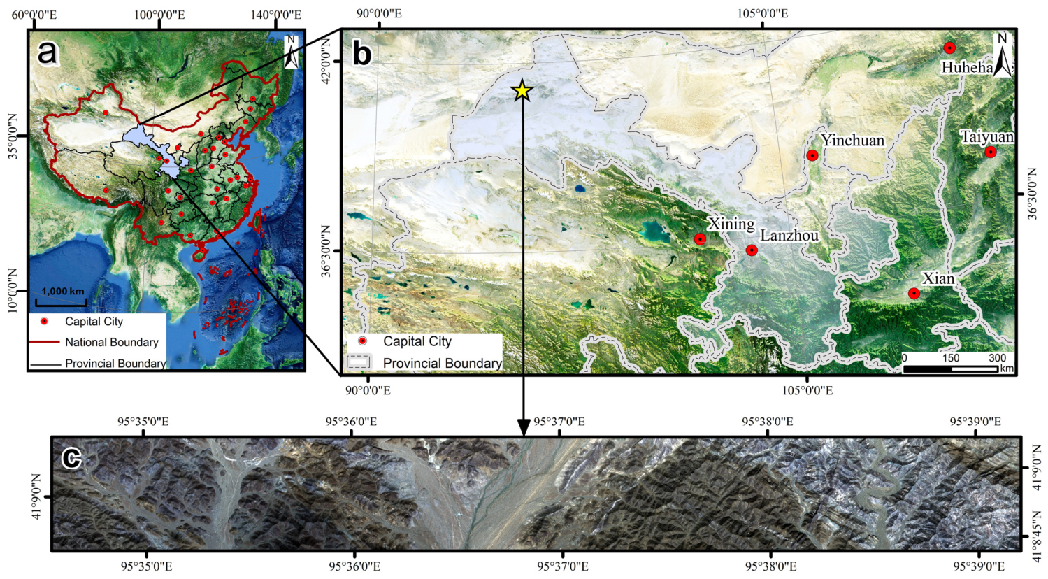
The study area is located in the Liuyuan region of Jiuquan City, Gansu Province, China, with an average elevation of 1797 m. It covers approximately 6.52 km
2, extending from 95°34′15″E to 95°39′30″E and 41°8′45″N to 41°9′15″N. The area is characterized by extensive bedrock exposure and can be classified as a bedrock-exposed zone. Well-developed alteration belts are widely exposed, providing favorable conditions for hyperspectral remote sensing of alteration minerals [
35]. The location of the study area is shown in
Figure 1.
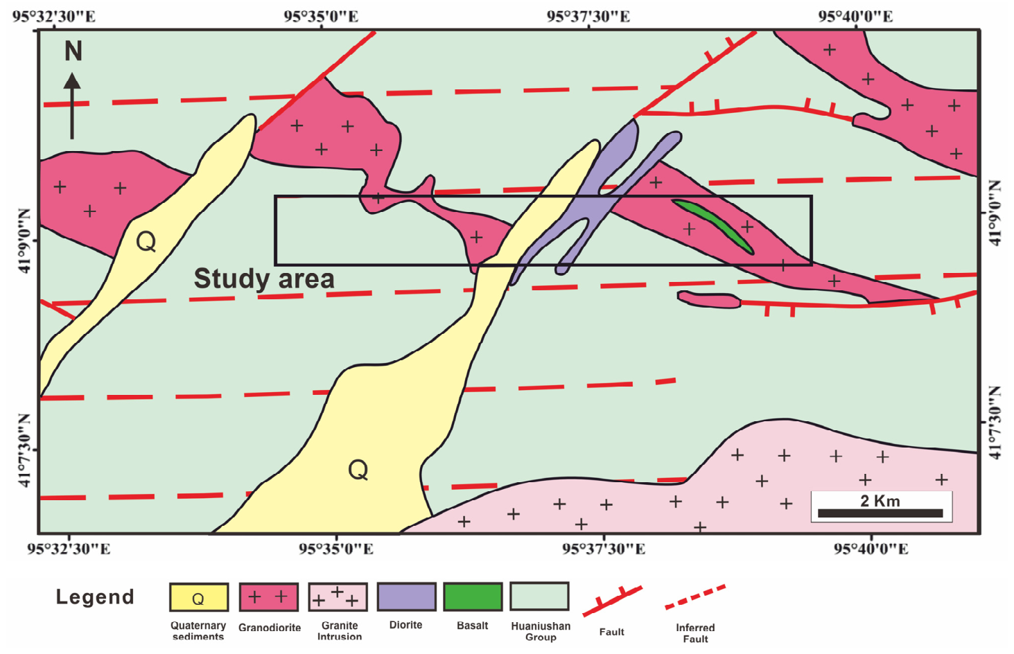
The stratigraphy of the study area consists of two group-level units: the Lower Silurian Xiashan Group (S1xsb) and the Middle-Upper Silurian Gongpoquan Group (S2–3gn). These units are mainly distributed between the Hongliuyuan Fault to the north and the Huaniuoshan–Chake’erhuduge Fault to the south. Their contact relationship is controlled by faulting. The Silurian strata have undergone a relatively high degree of metamorphism. Subsequent magmatic intrusion and tectonic deformation have further fragmented their spatial distribution.
The upper part of the Xiashan Group (S1xsb) is composed of a deeply metamorphosed sedimentary assemblage dominated by carbonate rocks. The lithological sequence mainly includes banded marble intercalated with mica-quartz schist, plagioclase amphibolite, and amphibole–biotite–muscovite schist, with a visible thickness of approximately 671.5 m. In contrast, the Gongpoquan Group (S2–3gn) represents a suite of volcanic–sedimentary rocks. It is primarily composed of weakly metamorphosed acidic volcanic lavas interbedded with terrigenous clastic rocks. Regionally, it also contains intercalations of schist, sandy slate, and basalt, with a thickness exceeding 774.3 m.
Magmatic activity in the study area is widespread and intensive. The lithology ranges from ultrabasic to acidic compositions, with granite and diorite being the most widely distributed. Intrusive bodies vary in scale and predominantly occur as batholiths, stocks, and dikes. Diorite and diabase dikes are commonly observed in clusters within host rocks. These intrusions, mainly in the form of stocks, have been placed into both the Xiashan Group and the Gongpoquan Group.
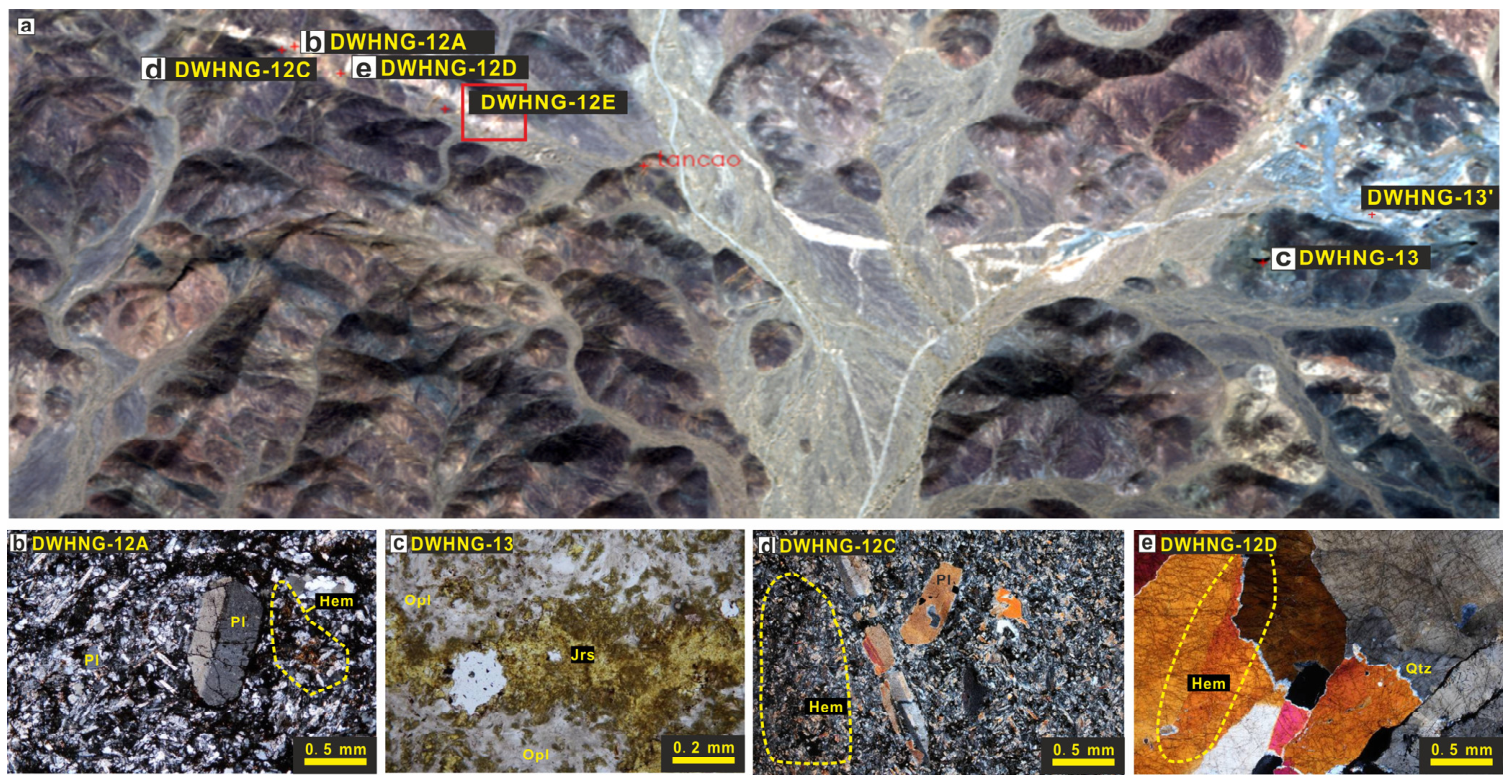
The lithological and structural heterogeneity in the study area has promoted the formation of iron-bearing hydrothermal alteration minerals, such as hematite, goethite, and jarosite, which occur as spatially fragmented surface exposures. These geological characteristics are important in this study because they generate both spectrally similar mineral assemblages and complex spatial patterns, posing significant challenges for airborne alteration mineral mapping. The geological overview map of the study area is shown in
Figure 2.
2.2. CASI Data and Preprocessing
Airborne hyperspectral data acquired by the Compact Airborne Spectrographic Imager (CASI) were used for alteration mineral mapping in the study area. The CASI sensor operates in the visible and near-infrared (VNIR) spectral range. The dataset was collected using the CASI-1500 imaging spectrometer (ITRES Research Limited, Calgary, AB, Canada), operated by the Beijing Research Institute of Uranium Geology, with a manned helicopter as the carrier platform. Data acquisition was conducted on 7–8 September 2010, during two flight campaigns. The aircraft maintained an average flight speed of approximately 60 m/s and a relative altitude of about 1800 m. Under these conditions, the spatial resolution of the CASI imagery is approximately 0.9 m. The main technical specifications of the sensor are summarized in
Table 1.
Prior to analysis, the CASI data were preprocessed to ensure radiometric and geometric consistency. Atmospheric correction was performed using the empirical line method (ELM), based on synchronous field-measured spectra collected at calibration sites within the study area. The relationship between airborne observations and ground reference spectra was applied to retrieve surface reflectance from the imagery. Subsequently, geometric correction and orthorectification were conducted using the ASTER 30 m digital elevation model (DEM) in conjunction with ground control points (GCPs), thereby reducing distortions caused by terrain effects and platform motion.
3. Methodology
3.1. The Flowchart of the Paper
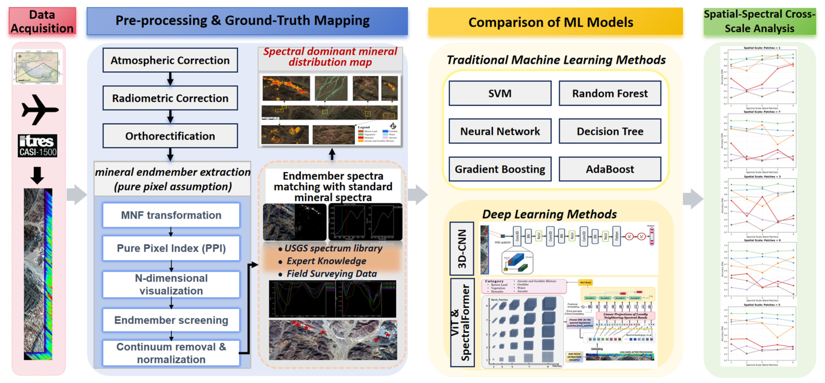
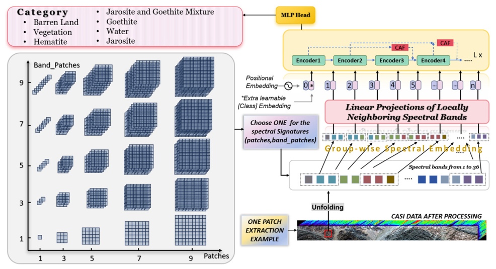
Figure 3 illustrates the overall workflow of the proposed collaborative alteration mineral mapping framework. The framework integrates geological knowledge with data-driven modeling and consists of four main stages: data preprocessing, expert-guided sample construction, model training and comparison, and multi-scale mechanism analysis.
In the third stage, the constructed dataset is used to train and evaluate different models. In addition to conventional convolutional neural networks (CNNs), a Transformer-based architecture, SpectralFormer, is introduced to model spectral dependencies. The model includes a Groupwise Spectral Embedding (GSE) module, which groups adjacent spectral bands to preserve local spectral continuity, and a Cross-layer Adaptive Fusion (CAF) module, which integrates hierarchical features across network layers. In the final stage, a multi-scale analysis is conducted to examine the influence of spectral and spatial representations on alteration mineral identification. The models are evaluated under different spatial patch sizes (1, 3, 5, 7, and 9) and spectral band group settings (1, 3, 5, 7, and 9). This analysis reveals the sensitivity of mineral classes to spatial–spectral information and supports the generation of a refined mineral distribution map.
3.2. Semi-Automatic Mineral Label Construction
Reliable pixel-level labels are essential for mineral classification in airborne hyperspectral studies, where direct field observations are spatially limited. In heterogeneous geological environments, most pixels represent varying degrees of mineral mixtures rather than pure endmembers. To address this issue, a semi-automatic labeling procedure was implemented within the Spectral Hourglass framework in ENVI 5.3. This approach integrates statistical endmember extraction with validation based on standard spectral libraries, expert knowledge, and field survey data.
The CASI datasets used in this study contain 36 spectral bands in the visible and near-infrared (VNIR) region with a spatial dimension of 7394 × 882 pixels. Prior to further processing, all bands were evaluated in terms of signal-to-noise ratio (SNR), and noisy channels were removed. Low-SNR bands at the spectral edges, as well as those affected by the water vapor absorption near 940 nm, were excluded. To improve spectral separability, a Minimum Noise Fraction (MNF) [
37] transformation was applied to reorganize the data according to signal-to-noise characteristics. Spectrally extreme pixels were then identified using the Pixel Purity Index (PPI) [
38], which detects candidate endmembers through random projections in high-dimensional spectral space. Clustering of these pixels produced a set of representative image endmembers for subsequent mineral identification.
The extracted endmembers were further used for mineral detection through Mixture Tuned Matched Filtering (MTMF). This approach enhances the detectability of target minerals while suppressing background variability. To ensure mineralogical reliability, the image endmembers were compared with reference spectra from the USGS spectral library [
39]. Diagnostic absorption positions and spectral shapes were examined to confirm mineral identity. Because several minerals exhibit partially overlapping absorption features in the VNIR region, additional refinement was conducted using HypPy (v3.0.1) [
40]. Expert knowledge was incorporated at this step to improve classification consistency. As summarized in
Table 2, hematite typically exhibits an absorption feature near 860–880 nm, goethite shows a broader feature around 900–920 nm, and jarosite is characterized by absorption features near 430 nm and approximately 900 nm associated with ferric-iron electronic transitions.
Through the integration of endmember extraction, spectral library comparison, and absorption feature analysis, a high-confidence mineral label dataset was constructed. The resulting samples exhibit clear spectral separability and geological consistency, providing reliable training data for subsequent classification.
Field investigations were conducted to further evaluate the geological reliability of the training samples. The surveyed alteration zone is located in the northwestern part of the study area (
Figure 4). Field observations identified hydrothermal alteration minerals including limonite, hematite, sericite, and jarosite. Representative rock samples were analyzed using petrographic microscopy at the Regional Geological Survey Institute of the Hebei Bureau of Geology and Mineral Resources.
More specifically, sample DWHNG-12A (
Figure 4b) was identified in the field as a red alteration rock. Laboratory analysis indicated that secondary minerals, including quartz, limonite, and sericite, account for approximately 15% of the total mineral composition. Sample DWHNG-13 (
Figure 4c) was predominantly jarosite (55–60%) and opal (40–45%), with sericite present as a minor phase. Sample DWHNG-12C (
Figure 4d) was described in the field as a limonitized rock and was subsequently identified under the microscope as a metamorphosed quartz monzodiorite porphyry containing secondary limonite. Sample DWHNG-12D (
Figure 4e) was identified petrographically as tourmaline-bearing secondary quartzite (vein type), with limonite occurring as a secondary mineral. The consistency between hyperspectral mineral mapping results and independent petrographic observations further confirms the geological reliability of the constructed ground-truth dataset and supports its use in subsequent mineral classification.
3.3. Machine Learning Models for Mineral Classification
3.3.1. Shallow Machine Learning Models
To provide a baseline for comparison with deep learning approaches, six representative shallow machine learning models were evaluated for mineral classification. All models were implemented using the Scikit-learn library and trained on the same stratified dataset, with 80% of the labeled samples used for training and 20% reserved for testing. A fixed random seed (random_state = 42) was adopted to ensure reproducibility. Model performance was assessed using Overall Accuracy (OA), Average Accuracy (AA), and Cohen’s Kappa coefficient [
42], together with class-wise precision to account for class imbalance.
A Support Vector Machine (SVM) with a radial basis function (RBF) kernel was used as a standard baseline for hyperspectral classification. In addition, several tree-based methods were evaluated due to their robustness to high-dimensional spectral data. These include a Decision Tree (DT) [
43], a Random Forest (RF) with 100 trees, and two boosting-based approaches: Gradient Boosting (GB), configured with 100 trees, a learning rate of 0.1, and a maximum depth of 3, and AdaBoost (AB), which combines 100 weak learners with a learning rate of 1.0. Finally, a Multilayer Perceptron (MLP) with a single hidden layer of 100 neurons was implemented using the Adam optimizer, with a maximum of 300 iterations, to provide a shallow neural network baseline.
3.3.2. 3D Convolutional Neural Network (3D-CNN)
Shallow machine learning methods treat each pixel independently and consider spectral bands as separate features. This limits their ability to capture spatial continuity in geological formations. To address this limitation, a three-dimensional convolutional neural network (3D-CNN) [
44] was employed. Unlike conventional 2D CNNs, the 3D-CNN performs convolution jointly across spatial and spectral dimensions, enabling integrated spectral–spatial feature extraction [
45].
The CASI hyperspectral dataset contains 36 spectral bands in the visible–near-infrared (VNIR) region. To reduce redundancy and computational cost, Principal Component Analysis (PCA) [
46] was applied, and the first 20 principal components were retained, accounting for more than 99.5% of the cumulative variance. The transformed data cube was then divided into overlapping three-dimensional patches of size 9 × 9 pixels, which serve as input samples for the network. The dataset includes seven land-cover and mineral classes and exhibits noticeable class imbalance. To ensure a fair evaluation, the data were first split into training (80%) and testing (20%) subsets. The Synthetic Minority Over-sampling Technique (SMOTE) [
47] was then applied to the training data to enhance the representation of minority classes and improve model generalization.
The adopted 3D-CNN architecture consists of three convolutional blocks followed by two fully connected layers. The first convolutional layer applies eight 3D kernels of size (3 × 3 × 3) to extract low-level spectral–spatial features. The second and third layers increase the number of feature channels to 16 and 32, using kernel sizes of (5 × 3 × 3) to progressively enlarge the receptive field and capture more complex spectral–spatial patterns. Each convolutional layer is followed by batch normalization and a ReLU activation function to stabilize training and introduce nonlinearity. After the final convolutional layer, the feature maps are flattened and passed through a fully connected layer with 512 neurons, followed by the output layer that produces class probabilities for the seven categories.
The network was implemented using the PyTorch (v2.4.1) framework. Model parameters were initialized from a normal distribution. Training was performed using the Adam optimizer with an initial learning rate of 0.001. A multiplicative learning-rate decay strategy (decay factor 0.97) was applied at each epoch to facilitate stable convergence. The model was trained for 20 epochs with a batch size of 10,000, and optimization was guided by the cross-entropy loss function. Classification performance was evaluated using Overall Accuracy (OA), Average Accuracy (AA), and the Cohen’s Kappa coefficient. The trained model was subsequently applied to the entire hyperspectral scene to produce a mineral classification map.
3.3.3. SpectralFormer-Based Mineral Classification Model
Hyperspectral reflectance spectra can be naturally interpreted as ordered spectral sequences. Capturing the dependencies among both adjacent and distant spectral bands is therefore essential for reliable mineral discrimination [
48,
49]. In this study, SpectralFormer [
50] is adopted as the core deep learning architecture to model hyperspectral spectral sequences for mineral classification.
Unlike convolutional neural networks, which primarily emphasize spatial locality, SpectralFormer approaches hyperspectral classification from a spectral sequence modeling perspective. It treats contiguous spectral bands as ordered tokens and learns long-range spectral dependencies through transformer-based attention mechanisms. The architecture employed in this study is illustrated in
Figure 5. The model is implemented in PyTorch. Two key parameters—spatial patch size (patches) and spectral grouping width (band_patches)—are systematically varied to examine their coupled influence on classification performance. This design enables a controlled transition from pixel-wise spectral modeling to joint spectral–spatial learning, allowing a unified analysis of scale effects in hyperspectral mineral mapping.
The main components of the model are described below.
- (1)
Spectral–Spatial Input Representation
Given a preprocessed hyperspectral cube , where H, W denote spatial dimensions and B is the number of spectral bands, two complementary input representations are considered: spatial patches and spectral groups. For the spatial–spectral setting, a local neighborhood centered at pixel is extracted as a spatial patch , where S denotes the spatial window size. The spatial patch is then flattened along the spatial dimension to form a spectral vector , which preserves the original spectral ordering while embedding local spatial context.
- (2)
Group-wise Spectral Embedding (GSE)
A key characteristic of hyperspectral data is the strong correlation among neighboring spectral bands. Treating each band independently may disrupt this continuity. To address this, SpectralFormer introduces a Group-wise Spectral Embedding (GSE) mechanism to model locally contiguous spectral segments.
A sliding window with width
(denoted as band_patches) is applied to the spectral vector to construct overlapping spectral groups. The
-th spectral group is defined as:
where
denotes the starting spectral index and
represents the number of neighboring bands within each spectral group. Each spectral group is then projected into a shared embedding space through a linear transformation:
where
is the learnable embedding matrix;
is the bias term; and
denotes the embedding dimension. The parameter
controls the local spectral context incorporated into each token. Adjusting this parameter enables systematic analysis of how spectral continuity influences mineral discrimination, which is particularly important for minerals such as iron oxides and sulfates whose diagnostic absorption features are often subtle and partially overlapping.
- (3)
Transformer Encoder with Cross-layer Adaptive Fusion
The embedded spectral tokens are augmented with positional encodings and passed through a stack of transformer encoder layers. Each encoder consists of a Multi-head Self-attention (MHSA) module followed by a Feed-forward Network (FFN) [
51,
52]. The attention operation is formulated as:
where
,
, and
denote the query, key, and value matrices, respectively, and
is the dimensionality of the key vectors.
To mitigate information degradation in deep transformer stacks and enhance spectral feature reuse, a Cross-layer Adaptive Fusion (CAF) mechanism is introduced. This module adaptively fuses representations from non-adjacent layers:
where
denotes the feature representation of the
layer and
is a learnable coefficient controlling the relative contribution of shallow and deep features. This fusion strategy helps preserve diagnostic spectral information that may otherwise degrade during deep feature propagation. It is particularly beneficial for minority mineral classes with limited training samples. After transformer encoding, the output tokens corresponding to the learned class token aggregate global spectral information and are fed into a multilayer perceptron (MLP) classifier:
where
is the predicted probability vector for the seven mineral and landcover classes;
and
denote the learnable parameters of the classification head; and
represents the embedding vector associated with the class token after transformer encoding.
4. Results
4.1. Ground-Truth Label Construction and Spatial Characteristics
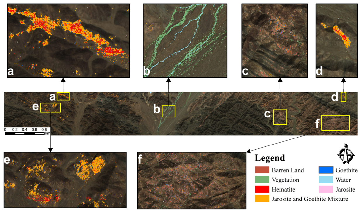
Ground-truth labels for major land-cover types and representative hydrothermal alteration minerals were derived from airborne CASI hyperspectral imagery, supported by field observations and expert geological interpretation. The resulting dataset comprises seven categories: barren land, vegetation, water, hematite, goethite, jarosite, and a jarosite–goethite mixture. Their spatial distribution is illustrated in
Figure 6. The labeled classes exhibit distinct spatial patterns that are closely linked to local geomorphological and structural controls.
Hematite occurrences are primarily concentrated in banded and patch-like structures, as shown by the red regions in
Figure 6a,d,e. In several locations, these occurrences form relatively continuous zones that follow the orientation of structural alteration belts. This pattern likely reflects the influence of hydrothermal fluid pathways and subsequent oxidation processes. Compared with hematite, goethite exhibits a more dispersed distribution pattern and typically appears as discontinuous spots or small patches (
Figure 6a,e,f). These occurrences are often embedded within areas dominated by other alteration minerals and are characterized by limited spatial extent and fragmented distribution.
Mixed zones consisting of jarosite and goethite are mainly located along the margins of hematite-rich regions (
Figure 6a,d,e). These areas display mosaic-like spatial textures that suggest gradual transitions in mineral assemblages under varying oxidation and weathering conditions. The spectral composition of these zones is relatively complex due to the coexistence of multiple alteration minerals, making them representative mixed-pixel regions in hyperspectral imagery. Jarosite itself generally occurs as isolated points or small clusters (
Figure 6c,f), with weak spatial continuity and relatively limited coverage. This distribution results in a relatively small number of labeled samples for this mineral category.
In addition to alteration minerals, three background classes were defined to characterize the broader land-cover context. Barren land occupies the largest proportion of the study area and forms spatially continuous surfaces (
Figure 6c,f). Vegetation is mainly distributed along valleys and low-lying areas where moisture conditions are favorable, forming linear or belt-like patterns that closely follow drainage features (
Figure 6b). Water bodies appear as narrow linear features with stable spatial locations and relatively homogeneous spectral responses, making them readily distinguishable from surrounding land-cover types.
Overall, the constructed ground-truth dataset captures the spatial morphology, distribution scale, and geological associations of the principal mineral and land-cover classes in the study area. These characteristics provide a reliable reference for evaluating the performance of different machine learning and deep learning approaches and for investigating spectral–spatial scale effects in airborne hyperspectral mineral classification.
4.2. Comparative Analysis of Different Machine Learning Methods
Table 3 summarizes the classification performance of representative shallow machine learning models and deep learning architectures on the CASI dataset. In addition to global metrics, including Overall Accuracy (OA), Average Accuracy (AA), and the Kappa coefficient, class-wise accuracies are also reported to assess each model’s ability to identify both dominant land-cover and relatively rare alteration minerals.
Among the traditional classifiers, the Support Vector Machine (SVM) achieved the best overall performance, with an OA of 94.62% and a Kappa coefficient of 0.9281. High accuracies were obtained for several dominant classes, including Classes 1, 2, 4, and 6, all exceeding 93%. However, its performance degraded markedly for minority classes. In particular, the accuracy for Class 7 (Jarosite) was zero, indicating a complete failure to detect this rare mineral under the imbalanced sample distribution.
Random Forest (RF) produced relatively stable performance for dominant classes but showed reduced accuracy for several minority categories, leading to a lower AA of 55.54%. Other ensemble methods, including Gradient Boosting and AdaBoost, exhibited similar limitations when handling spectrally similar mineral classes, with OA values of 82.29% and 76.92%, respectively.
Deep learning models incorporate joint spatial–spectral information during classification. The 3D-CNN model achieved an OA of 86.26% and an AA of 67.35%, outperforming several traditional ensemble methods. In contrast, the Vision Transformer (ViT) yielded a lower OA of 71.28%, suggesting that a standard transformer architecture may not fully effectively capture hyperspectral spectral characteristics without task-specific adaptation.
The SpectralFormer model was further evaluated under different spectral grouping settings. Although its overall OA (82% under the optimal configuration) remained lower than that of the SVM baseline, it showed improved reliability for several challenging mineral categories. For example, the classification accuracy for Hematite (Class 3) reached 97% under the band_patches = 7 setting, while Goethite (Class 5) achieved an accuracy of 82% with band_patches = 9. For the rare Jarosite class (Class 7), SpectralFormer consistently produced non-zero accuracy, whereas several baseline models failed to identify this category.
In addition to the quantitative comparison presented in
Table 3,
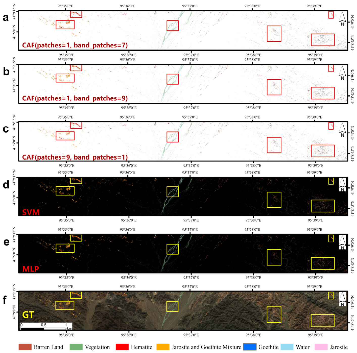
Figure 7 presents the spatial distribution of classification results obtained from different models. Overall, all methods reproduce similar large-scale spatial patterns. This is particularly evident in regions dominated by barren land, vegetation, and major alteration zones. Such consistency indicates that most models can capture the primary land-cover structure of the study area.
Differences become more apparent at the local scale, as highlighted by the yellow boxes in
Figure 7. The SpectralFormer models under different parameter configurations (
Figure 7a–c) produce highly consistent spatial patterns. This suggests that moderate variations in spectral grouping and spatial patch size have limited impact on the overall structural representation. The SVM and MLP results (
Figure 7d,e) are also broadly consistent with the ground-truth reference (
Figure 7f). However, discrepancies emerge in areas containing fragmented mineral occurrences or small alteration patches. In these regions, models differ in spatial continuity and exhibit varying levels of classification noise.
Overall, despite differences in quantitative metrics, the major geological patterns are consistently reproduced across models. The primary variations are confined to small-scale mineral occurrences and boundary regions, where spatial fragmentation and spectral ambiguity are more pronounced.
4.3. Multi-Scale Spectral–Spatial Classification Accuracy Based on SpectralFormer
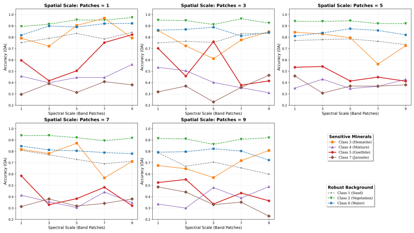
Figure 8 illustrates class-wise classification accuracy under varying spectral grouping and spatial patch configurations using the SpectralFormer model. The results show clear differences in scale sensitivity among background classes and alteration minerals.
Background classes, including barren land (Class 1), vegetation (Class 2), and water (Class 6), maintain high accuracies across almost all configurations. Only minor fluctuations are observed with increasing patch size, indicating that these classes are largely insensitive to spectral–spatial scale variations.
In contrast, alteration minerals exhibit stronger scale dependence. When spatial patch size is minimal (patches = 1), increasing the spectral grouping scale generally improves the classification accuracy of hematite (Class 3) and goethite (Class 5). Their performance typically peaks at intermediate to large spectral grouping levels (band patches = 7–9). However, this trend is not observed for the mixture class (Class 4), which shows limited sensitivity to spectral scaling.
When the spectral grouping is fixed, introducing moderate spatial context (patch sizes = 3–5) provides slight performance improvements for several mineral classes. However, further increasing the spatial window (patch sizes = 7–9) often leads to a decline in accuracy. This effect is particularly evident for minerals with fragmented spatial distributions, where larger neighborhoods introduce heterogeneous background signals.
No single spectral–spatial configuration performs optimally across all classes. The jarosite class (Class 7), despite its limited representation, maintains detectable accuracy under most configurations, This suggests a certain degree of robustness in its feature representation. Overall, these results indicate that classification performance is jointly controlled by spectral grouping and spatial context. Different classes exhibit distinct sensitivities to scale variations, reflecting their inherent spectral characteristics and spatial distribution patterns.
5. Discussion
5.1. Comparative Implications of Shallow and Deep Models for Mineral Mapping
The results presented in
Table 1 reveal a clear discrepancy between global evaluation metrics and class-wise performance. Models such as SVM achieve high overall accuracy, mainly due to their strong performance on dominant background classes. These classes occupy large spatial extents and exhibit clear spectral separability, which tends to bias global metrics.
However, this advantage does not extend to alteration mineral discrimination. For minerals with limited spatial coverage or subtle spectral differences, the performance of shallow models declines markedly. Classes such as jarosite and goethite show low recall and unstable predictions, indicating that pixel-wise decision boundaries are insufficient in such cases. Ensemble methods, including Random Forest and boosting-based approaches, improve robustness to some extent, but their gains are mainly reflected in majority classes rather than in rare or spectrally ambiguous categories.
Deep learning models introduce spatial context into the classification process and partially alleviate this limitation. The 3D-CNN produces more balanced class-wise results by incorporating local neighborhoods and reducing noise. However, its fixed receptive field limits its ability to capture long-range spectral dependencies. The standard ViT, although capable of modeling global relationships, performs less effectively in this task. Treating spectral bands as independent tokens disrupts the continuity, which weakens the representation of diagnostic absorption features.
In comparison, SpectralFormer exhibits more stable behavior across mineral classes. Its advantage is reflected not in overall accuracy but in its ability to maintain consistent predictions for spectrally subtle and low-frequency classes. For example, the non-zero detection of jarosite across different configurations suggests that preserving spectral continuity is more important than simply increasing spatial coverage.
Overall, the results indicate that model performance in hyperspectral mineral mapping is not determined by architectural complexity alone. Instead, it depends more strongly on how spectral characteristics are represented and how spatial context is incorporated. This observation is consistent with previous studies [
53,
54], which report that increased model complexity does not necessarily lead to improved predictive performance.
5.2. Scale-Effect Mechanism Explanation in Spectral–Spatial Mineral Classification
The multi-scale analysis shows that classification performance does not vary monotonically with spectral or spatial scale. Increasing spectral grouping or enlarging spatial context does not consistently improve results, and the responses differ across mineral classes.
For minerals such as hematite and goethite, performance is closely linked to spectral continuity. Increasing the spectral grouping scale allows the model to capture broader inter-band relationships, which helps stabilize absorption-related features. This is particularly evident when spatial context is limited, where spectral information plays a dominant role. However, this trend weakens as spatial context increases. For several mineral classes, enlarging the spatial window leads to reduced accuracy. This effect is more pronounced for minerals with discontinuous or vein-like distributions, where larger neighborhoods introduce heterogeneous background signals. In such cases, spatial aggregation tends to weaken class-specific spectral characteristics. The mixture class exhibits a different pattern. Its response to both spectral and spatial scaling remains limited. This behavior may be related to the absence of stable diagnostic features and the influence of sub-pixel mixing. It suggests that neither spectral sequence modeling nor spatial context alone is sufficient for such categories.
In contrast, background classes remain stable across all configurations. This provides a useful reference, indicating that the observed scale effects are not caused by model instability but are related to intrinsic differences between classes. Taken together, the results highlight a trade-off between spectral representation and spatial aggregation. For alteration minerals, preserving spectral structure appears more critical than expanding spatial context, although moderate spatial information can still help reduce noise.
It should also be noted that the observed scale effects are influenced by the quality of training samples. In airborne hyperspectral mineral mapping, it is difficult to ensure that all samples correspond to spectrally pure mineral pixels, especially under strong sub-pixel mixing and spatial fragmentation. As reported in previous studies [
19], some degree of sample noise is often unavoidable when constructing sufficiently large training datasets. This limitation introduces uncertainty and may partly explain the variability observed across different spectral–spatial configurations.
Despite this constraint, the results suggest that integrating spectral and spatial representations can still improve mineral discrimination. In particular, spectral continuity plays a primary role, while spatial context provides complementary information for noise suppression. Future work may focus on individual mineral types, with more detailed analyses of scale-dependent spectral characteristics and spatial distribution patterns. Such efforts could further refine the balance between spectral and spatial representations and improve the robustness of hyperspectral mineral mapping.
5.3. Limitations and Future Research
Several limitations should be acknowledged. First, our experiments are based on a single airborne CASI dataset. The observed scale-dependent behaviors might vary under different sensor characteristics, spectral resolutions, or geological settings. Additional datasets are needed to assess the generalizability of the findings. Second, although SpectralFormer shows relatively stable performance for minority classes, it is not specifically designed to address severe class imbalance. Future work could incorporate adaptive weighting strategies or class-aware optimization methods to better handle highly imbalanced datasets. Third, the current framework relies entirely on supervised learning. Constructing high-quality, pixel-level training data remains labor-intensive. Self-supervised approaches such as Masked Autoencoders (MAE) [
55,
56] provide a promising direction for reducing labeling costs while improving generalization. Fourth, this study focuses on a localized area and lacks quantitative mineralogical constraints. Future large-scale studies should incorporate analytical techniques such as X-ray diffraction (XRD), to provide more rigorous validation.
6. Conclusions
This study examines the spectral–spatial mechanisms governing mineral identification from airborne hyperspectral data in the context of complex alteration mapping. By integrating geologically constrained samples, multi-model comparisons, and scale-aware analyses, the primary findings can be summarized as follows.
A primary observation is that overall accuracy alone provides a limited and potentially misleading assessment of mapping performance. Although pixel-wise shallow classifiers yield high global accuracy, they consistently underperform in detecting rare and spectrally ambiguous minerals, reflecting a systematic bias toward dominant background classes. This behavior highlights the intrinsic limitation of accuracy-driven evaluations under the severe class imbalance inherent to most geological datasets.
Furthermore, the influence of spatial context is inherently scale-dependent. Incorporating local spatial information improves robustness to noise; however, as the spatial support increases, diagnostic spectral features are progressively attenuated. This effect becomes particularly pronounced in highly fragmented alteration zones, where spatial aggregation obscures mineral-specific absorption characteristics. Such observations indicate that spatial context, while beneficial, must remain subordinate to the preservation of fundamental spectral structure.
Across multi-scale settings, mineral discrimination is consistently governed by a spectral-dominant mechanism. This trend holds across different model families, indicating that performance variations are primarily controlled by representation strategies rather than pure architectural complexity. Transformer-based models exhibit a distinct advantage in maintaining spectral continuity while adaptively incorporating spatial information. Moderate spectral grouping improves discrimination, whereas excessive spatial expansion reduces sensitivity due to increased background interference.
Taken together, these findings suggest a unified interpretation: mineral identification from airborne hyperspectral data is fundamentally constrained by the preservation of spectral continuity across varying spatial scales. Model performance reflects the extent to which this constraint is respected. This mechanistic perspective provides a robust foundation for understanding spectral–spatial interactions beyond specific deep learning implementations.