Deriving Deflection of the Vertical and Gravity Anomaly from SWOT/KaRIn Data Using an Optimized Discretization Method

Highlights

What are the main findings?

• An optimized discretization method (ODM) is developed to fully utilize the two-dimensional characteristics of SWOT/KaRIn data. It integrates multi-directional observations and higher-order numerical differentiation, providing a practical alternative method. It avoids complex covariance modeling and parameter estimation while achieving comparable accuracy. This makes the method easier to implement and more suitable for large-scale applications.
• The derived SWOT_DOV achieves high accuracy, with STDs of 1.60 μrad (north) and 2.02 μrad (east) against the SIO V32.1 model. Marine gravity anomaly (SWOT_GA) is derived using the inverse Vening-Meinesz formula. The STD of the differences between SWOT_GA and the NCEI shipborne gravity data is 3.85 mGal. Accuracy analyses show that high-quality gravity signals are mainly obtained in deep-ocean and offshore regions with gentle seafloor gradients.

What are the implications of the main findings?

• The ODM provides a simple, efficient, and robust alternative to the LSC method while improving data utilization. Exploiting multi-directional and higher-order information is critical for fully leveraging wide-swath altimetry data.
• SWOT performs well in recovering marine gravity anomalies in the open ocean and can support future geodetic and oceanographic studies.

Abstract

The Surface Water and Ocean Topography (SWOT) mission carries a Ka-band interferometric radar altimeter (KaRIn), which enables high-resolution wide-swath measurements of sea surface height, providing new opportunities for deriving high-precision marine gravity fields. The discretization method used by the Scripps Institution of Oceanography (SIO) is one of the simplest methods for deriving deflections of the vertical (DOV), as it avoids parameter estimation and complex mathematical procedures. However, this method only uses adjacent observations for first-order differentiation and ignores diagonal directions, resulting in relatively low data utilization for SWOT/KaRIn data. The optimized discretization method is proposed to take advantage of the two-dimensional characteristics of KaRIn data. Multi-directional data is introduced to estimate the DOV (SWOT_DOV), and the numerical differentiation strategy is extended to higher orders. These significantly improve the solution quality. The standard deviation (STD) of the differences between SWOT_DOV and north_32.1 is 1.60 μrad, and that with east_32.1 is 2.02 μrad. Gravity anomalies are further derived using the inverse Vening-Meinesz formula. Validation using NCEI shipborne gravity data indicates an STD of 3.85 mGal. Further analyses considering seafloor topography gradient, depth, and offshore distance demonstrate that SWOT/KaRIn data have a stable capability to restore high-precision marine gravity field features.

1. Introduction

With the development of satellite technology, more than twenty altimetry missions have contributed to oceanographic research [1]. Continuous improvements in altimetry technology have greatly enhanced the accuracy and coverage of sea surface observations [2,3,4,5,6,7]. Owing to its short repeat cycle and near-global spatial coverage, satellite altimetry data have become the primary data for deriving the marine gravity field [8,9,10,11,12].

High-resolution models of the deflection of the vertical (DOV) and marine gravity anomalies (GAs) can be derived from altimetry observations [13,14,15,16,17,18,19,20,21]. These products provide important geophysical information for seafloor topography and gravity gradients [14,15,22,23,24,25,26,27,28].

The Surface Water and Ocean Topography (SWOT) mission was successfully launched on 16 December 2022 (https://swot.jpl.nasa.gov/mission/launch/, (accessed on 16 December 2022)). It has attracted more attention, making it an important development in oceanographic research [11,15,16,17,29,30,31,32,33,34,35,36,37]. SWOT measures sea surface height (SSH) including along-track and across-track directions by interferometry, which help in understanding the ocean better than using one-dimensional along-track nadir data [34]. The wide-swath mode provides a large amount of SSH observations, which are highly accurate for deriving marine gravity field models [32,38].

Before the launch of SWOT, many studies have been conducted using simulated data. Wan et al. used a numerical derivation method to demonstrate that the two components of the DOV derived from simulated wide-swath data have nearly identical accuracy [33]. Yu et al. restored the GA from simulated SWOT wide-swath data using the Inverse Vening-Meinesz (IVM) formula and the Inverse Stokes Method [34]. Their results showed that IVM is more robust than ISM in handling both random and systematic errors in SWOT data.

Guo et al. used the SWOT beta-version product and applied the least-squares collocation (LSC) method to estimate the DOV and GA in the Bay of Bengal [14]. Results from only one-cycle L2 data are comparable to those obtained from long-term HY-2A and CryoSat-2 observations [5]. Li et al. used SWOT L3 products and applied a discretization method to calculate the DOV [17]. They stacked data from 27 cycles to estimate the DOV and GA. Validation against shipborne gravity data showed slightly better performance than the SIO grav_32.1 model. Zhu et al. used the moving geoid gradient method to recover the high-precision marine DOV and GA [21]. Zhu et al. calculated the GA by stacking 15-cycle L3 data in the South China Sea and then deriving the topography [39]. The results show that SWOT/KaRIn data is beneficial for higher-precision ocean gravity field modeling and applications. Guo et al. used 30-cycle L2 products to calculate the DOV by the LSC method in the Arabian Sea [13]. The results show an accuracy comparable to the SIO V32.1 model. Ya et al. stacked data from 20-cycle SWOT/KaRIn data and computed DOV using the LSC method [40]. Li et al. proposed an adaptive weighting method based on multi-directional SWOT/KaRIn data to estimate the DOV [41]. Feng et al. used existing SWOT-derived marine gravity models to recover a high-precision global bathymetry model by an improved gravity–geological method [42]. Wang et al. combined SWOT/KaRIn data with nadir altimetry to derive the DOV and GA models in the South China Sea [43].

Several methods are widely used to derive the marine DOV, including the least-squares method, the LSC method, and the discretization method. Among them, the discretization method is the simplest in terms of computational procedure. Several versions of the SIO DOV models are derived from it [18,35,36]. However, considering the characteristics of SWOT observations, the discretization method can still be further improved. The KaRIn altimeter provides a dense set of almost regular grid products. Based on these data, the DOV can be derived using central numerical differences from neighboring points. The gravity field is continuous and spatially correlated. The gravity signal at a given point is, therefore, influenced not only by the local mass distribution but also by the surrounding region.

In this study, the discretization method is further improved. A multi-directional and multi-scale central differencing strategy is introduced. Section 2 introduces the study area and the datasets. Section 3 presents the optimized discretization method (shortly named ODM) used to compute the DOV (shortly named SWOT_DOV), and also the IVM formula for deriving the GA model (shortly named SWOT_GA). In Section 4, the accuracy of SWOT_DOV and SWOT_GA is evaluated. And this part further analyzes the results of SWOT_GA considering seafloor topography gradient, depth, and offshore distance. Section 5 presents the discussion. Finally, Section 6 presents the conclusions.

2. Study Area and Data

2.1. Study Area

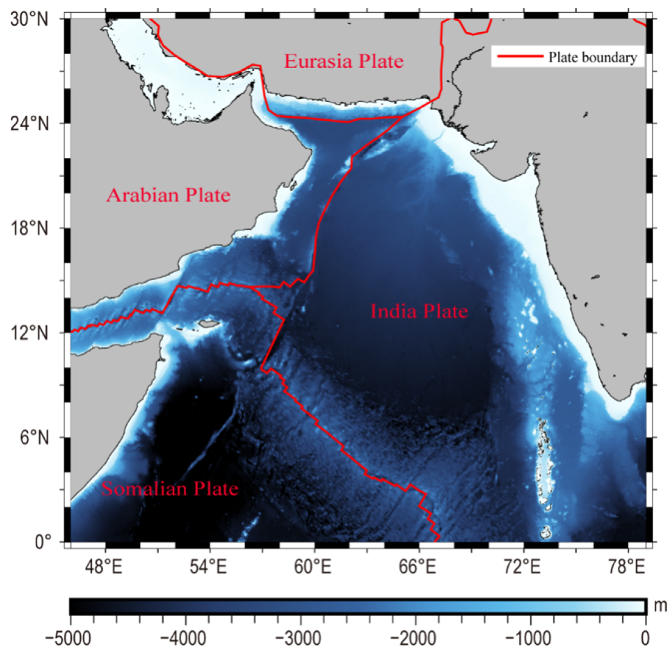
To compare this study with the experiments based on the LSC method by Guo & Wan [15], we select the same study area, the Arabian Sea (0–30°N, 46–79°E). The Arabian Sea is located in the North-Western Indian Ocean. It lies near the junction of the Somali, Indian, and Arabian plates [15]. Its topography results from the multiple influences of plate tectonics, sedimentation, and monsoon-driven circulation. As a result, the region exhibits pronounced spatial variability. It includes both smooth deep-ocean areas and steep gradients near the continental margin. This diversity provides an effective testbed for assessing the stability of the ODM. Figure 1 presents the bathymetry of the Arabian Sea from the topo_27.1 bathymetric model. The Owen Fracture Zone in the west and the Chagos–Laccadive Ridge in the east form a north–south structural barrier. These structures are located near the boundary between the Arabian and Indian plates [44]. The deep-sea plain in the eastern region is split by the Carlsberg Ridge into the Arabian Basin and the Somali Basin. Both basins reach maximum depths exceeding 4800 m [45]. The region is tectonically active and characterized by frequent seismic activity [46].

2.2. Data Source

The datasets used in this study are summarized in

Table 1. Information of datasets.

Datasets	Provider
SWOT L2_LR_KaRIn ssha_karin	CNES
Mean Sea Surface (MSS) MSS_CNES_CLS2022 (1′)	Technical University of Denmark (DTU)
Mean Dynamic topography (MDT) DTUUH22MDT (7.5′)	DTU
EGM2008	National Geospatial-Intelligence Agency (NGA)
SIO V32.1 datasets (1′)	SIO
grav_SWOT_04 (1′)
topo_27.1 (1′)
GMGA2 (1′)	China University of Geosciences (Beijing) (CUGB)
DTU21GRA (1′)	DTU
SDUST2022GRA (1′)	Shandong University of Science and Technology (SDUST)
NCEI gravity data	National Centres for Environmental Information (NCEI)

. The experiment is based on the SWOT/KaRIn L2 data [15]. To ensure a consistent comparison with Guo & Wan’s experiments, this study uses the same 30-cycle data (cycle_001~cycle_030) to estimate the DOV in the same study region. The dataset includes PGC0 cycle_001~cycle_009, PIC0 cycle_010~cycle_022, and PIC2 cycle_023~cycle_030. The observations span from 26 July 2023 to 7 April 2025, covering a period of approximately 21 months.

The datasets used in this study are summarized in Table 1. When selecting the MSS and the MDT model, their correlation should be minimized to avoid signal leakage and aliasing effects [47,48]. Following this principle, the MSS_CNES_CLS2022 and DTUUH22MDT models are used in combination.

EGM2008, provided by the NGA, is a global gravity field model that combines terrestrial gravity data, shipborne gravity data, satellite altimetry data, and GRACE satellite gravity data [49]. It provides reliable information for the long- and medium-wavelength components of the Earth’s gravity field [9]. And it is also used for the remove–calculate–restore procedure.

The SIO V32.1 dataset includes east_32.1, north_32.1, and grav_32.1, representing one of the most accurate global marine gravity models currently available [9,50,51]. It should be noted that the SIO group has recently released the updated V33.1 gravity products. However, to allow comparison with the results of Guo & Wan [15], only the V32.1 model is used in this study. The grav_SWOT_04 model is produced recently by SWOT/KaRIn data based on V32.1. In addition, a topography model is required for several validation analyses. The bathymetry model topo_27.1 is adopted.

The DTU21GRA is constructed using observations from multiple satellite altimetry missions. The model incorporates retracked SSH, updated geophysical corrections, and improved data editing procedures [52,53]. Geoid gradients are converted into DOV and gridded at a 1′ grid. DTU21GRA shows improved performance in recovering short-wavelength signals and in coastal regions [54]. A key feature of DTU21GRA is that residual SSH signals are directly incorporated into the GA inversion process [52]. This represents an important methodological difference from the discretization method used by SIO [50,51].

GMGA2 is a high-precision global marine GA model developed by CUGB [55]. It is based on the earlier GMGA1 model derived from conventional satellite altimetry data [55,56]. GMGA2 incorporates high-frequency gravity signals predicted from bathymetric data using the Parker forward modeling formula, which improves the accuracy of the model. The SDUST2022GRA model is developed by SDUST [10]. It is a global marine GA model with a spatial resolution of 1′. The model integrates observations from ICESat-2 multi-beam laser altimetry, low-resolution radar altimetry in Ku and Ka bands, and SAR-mode altimetry measurements.

Shipborne gravity data used for validation are obtained from the NCEI database. The NCEI dataset compiles marine gravity observations collected by multiple institutions using different instruments [57]. Since the 1990s, the accuracy of shipborne gravity measurements has improved significantly due to advances in navigation technology as well as improvements in measurement instruments. The accuracy of observation is now about 1–3 mGal [17].

3. Methodology

3.1. ODM for Deriving Marine DOV

In this study, the ODM is applied to estimate the gridded SWOT_DOV. SWOT_GA is then derived from the SWOT_DOV using the IVM formula [6,7,17,58,59]. The results are compared with those reported by Guo & Wan, who used the LSC method combined with IVM [15].

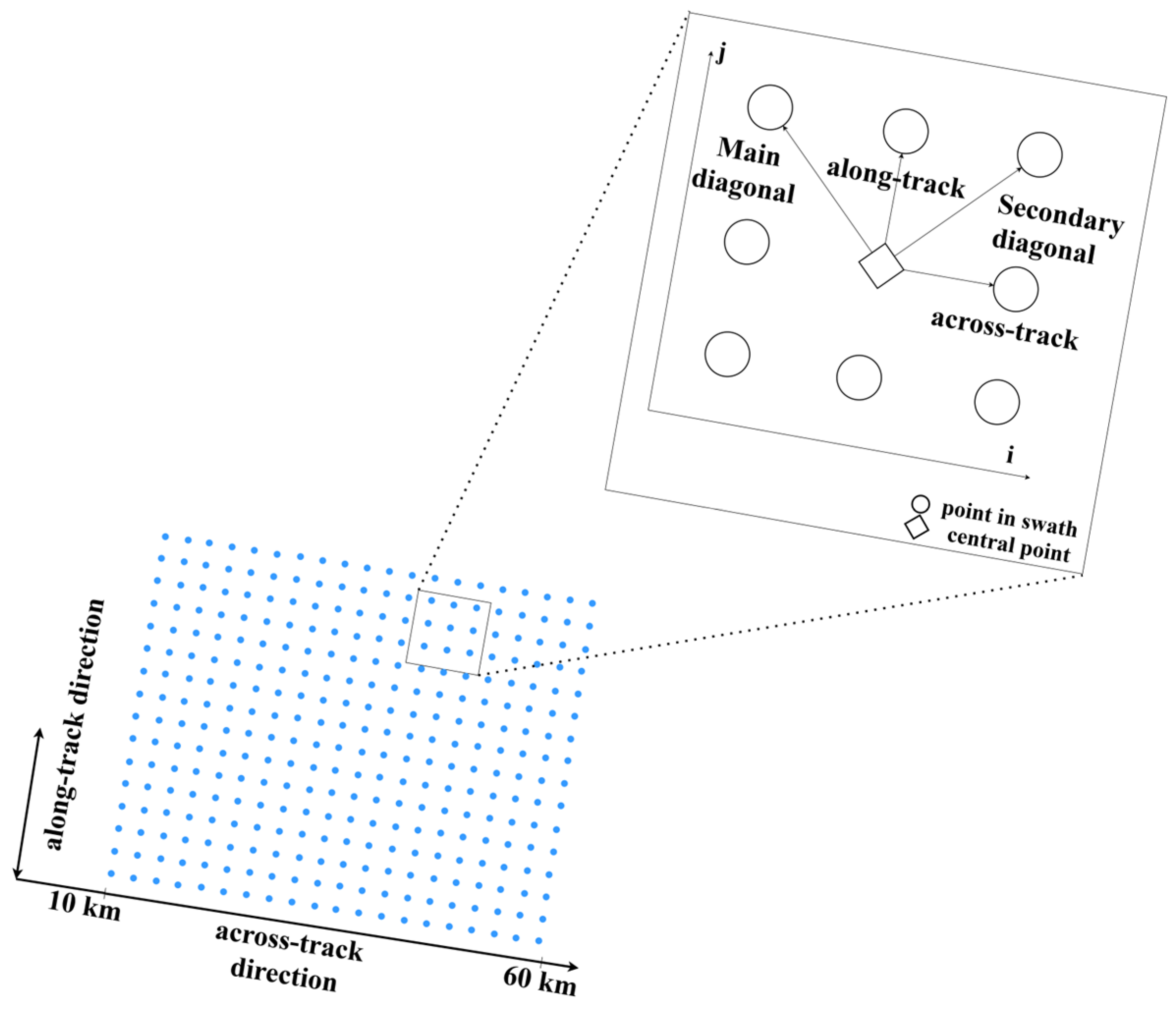
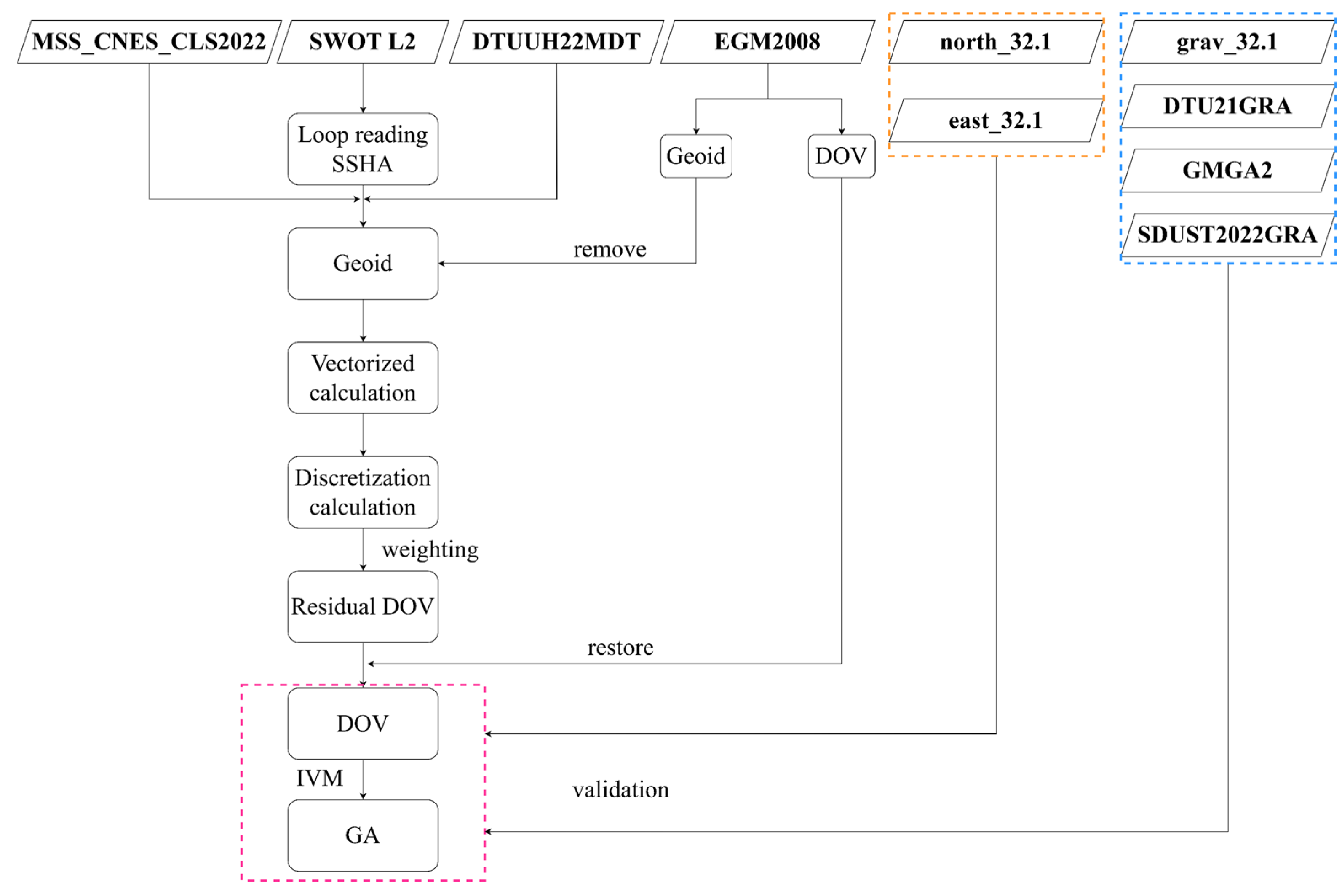
Following the wide-swath data processing strategy described by Tian [60] and Wan et al. [11], the SWOT/KaRIn data are directly used to compute the geoid by combining the MSS_CNES_CLS2022 and DTUUH22MDT. The data are then interpolated to standard grid nodes using the blockmedian module provided by the Generic Mapping Tool version 6.4 (GMT) [61], which effectively eliminates the occurrence of diamond-shaped gaps at the final DOV results. The data are further processed using an 8 km Gaussian filter to suppress high-frequency noise [35,36]. As shown in Figure 2, the blue points represent the ssha_karin from the L2 product, with a spacing of approximately 2 km. The zoomed-in subfigure illustrates the calculation of the DOV by the ODM. Although a local coordinate system is defined along the swath, it is introduced only for indexing and discretization purposes. It does not replace the geographic coordinate system. All observations retained its longitude and latitude information. Each data matrix is associated with a corresponding coordinate matrix, which stores the geographic position of every point. During vectorized computations by matrices, distances and directions between neighboring points are evaluated directly, ensuring that the spatial relationships are preserved. Therefore, no additional coordinate transformation is required. The overall experimental workflow is illustrated in Figure 3.

The geoid gradient $e$ and the DOV $\epsilon$ are computed based on the geoid heights and the spherical distance $\psi$ between the two points [62]:

$$e = -\epsilon = {\displaystyle \frac{\partial N}{\partial \psi }}$$

(1)

The $\xi$ and $\eta$ are the partial derivatives of the geoid height $N$ concerning the north–south and east–west directions [5,17,19]:

$$\left\{\begin{array}{l}\xi =-{\displaystyle \frac{\partial N}{\partial x}}=-{\displaystyle \frac{1}{R}}{\displaystyle \frac{\partial N}{\partial \phi }}\\ \eta =-{\displaystyle \frac{\partial N}{\partial y}}=-{\displaystyle \frac{1}{R\cos \phi }}{\displaystyle \frac{\partial N}{\partial \lambda }}\end{array}\right.$$

(2)

where $R$ denotes the mean radius of the Earth; $\phi$ and $\lambda$ represent the latitude and longitude of the grid point, respectively. When the two components of DOV are expressed in a differential form, the expressions can be obtained in Equation (3).

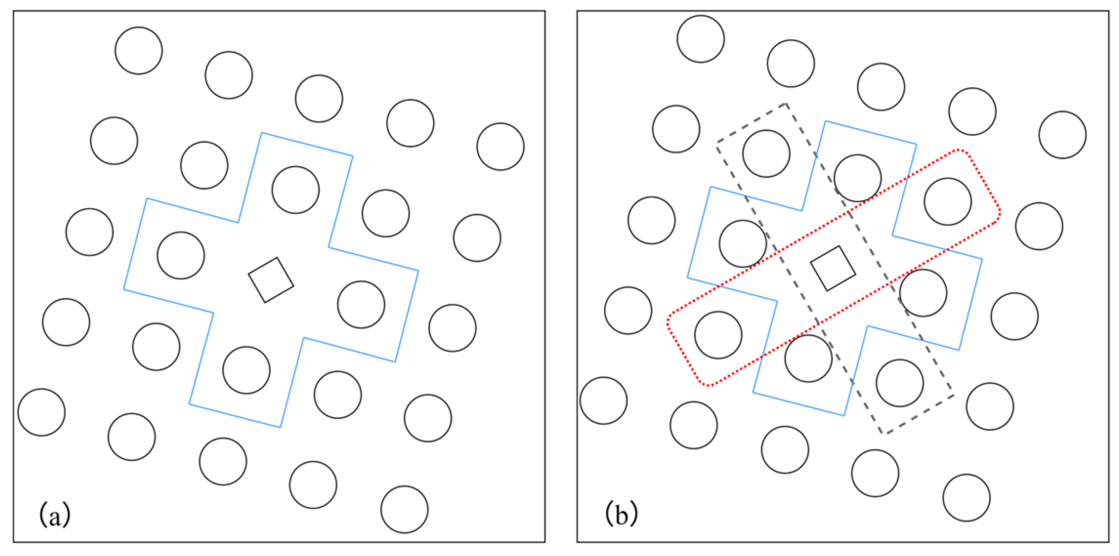
Figure 4 illustrates the use of multi-directional data for DOV estimation based on swath data. In Figure 4a, four-directional data are used (shortly named 4d), highlighted by a blue box. In Figure 4b, eight-directional data (8d) are employed. The dark-gray dashed box and the red dotted box indicate the additional diagonal directions introduced in the 8d scheme. The figure represents the data selection scheme for first-order numerical differentiation.

As shown in Figure 4a, the two components of the DOV are derived from 4d data by the central discretization method [11,24,50,60]:

$$\left\{\begin{array}{l}{\xi }_{\left(i,j\right)}=-{\displaystyle \frac{1}{R}}{\displaystyle \frac{\partial N_{\left(i,j\right)}}{\partial {\phi }_{\left(i,j\right)}}}=-{\displaystyle \frac{1}{R}}{\displaystyle \frac{N_{\left(i+1,j\right)}-N_{\left(i-1,j\right)}}{{\phi }_{\left(i+1,j\right)}-{\phi }_{\left(i-1,j\right)}}}\\ {\eta }_{\left(i,j\right)}=-{\displaystyle \frac{1}{R\cos {\phi }_{\left(i,j\right)}}}{\displaystyle \frac{\partial N_{\left(i,j\right)}}{\partial {\lambda }_{\left(i,j\right)}}}=-{\displaystyle \frac{1}{R\cos {\phi }_{\left(i,j\right)}}}{\displaystyle \frac{N_{\left(i,j+1\right)}-N_{\left(i,j-1\right)}}{{\lambda }_{\left(i,j+1\right)}-{\lambda }_{\left(i,j-1\right)}}}\end{array}\right.$$

(3)

The expression represents the DOV obtained by discretizing the data in the meridional and zonal directions around the central grid point, where the grid spacing is $k=1$. This formulation can be summarized as

$$\left\{\begin{array}{l}{f}_{\phi \left(i,j\right)}{|}_k=-{\displaystyle \frac{N_{\left(i+k,j\right)}-N_{\left(i-k,j\right)}}{R\cdot \Delta \phi }}\\ f_{\lambda \left(i,j\right)}{|}_k=-{\displaystyle \frac{N_{\left(i,j+k\right)}-N_{\left(i,j-k\right)}}{R\cos {\phi }_{\left(i,j\right)}\cdot \Delta \lambda }}\end{array}\right.$$

(4)

where $\Delta \phi$ represents the latitude difference between two grid points, and $\Delta \lambda$ denotes the longitude difference between the corresponding grid points.

Considering the contribution of the grid data along the two diagonal directions, Equation (4) can be further expressed as

$$\left\{\begin{array}{l}{\xi }_{\left(i,j\right)}{|}_k=-{\displaystyle \frac{1}{W}}{\displaystyle \sum _{k=1}^n{w}_k{f}_{\xi \left(i,j\right)}{|}_k}\\ {\eta }_{\left(i,j\right)}{|}_k=-{\displaystyle \frac{1}{W}}{\displaystyle \sum _{k=1}^n{w}_k{f}_{\eta \left(i,j\right)}{|}_k}\end{array}\right.$$

(5)

where $W$ denotes the inverse distance weighting (IDW) method; $W={\displaystyle \sum _{k=1}^n{w}_k}$, $w_k={\displaystyle \frac{1}{{d_k}^2}}$, $d_k$ represents the spherical distance between the central grid point and the neighbor points used in the calculation along the given direction. Using the IDW method accounts for both the distance between grid points and the local signal variability. The formulas for the two components of the DOV are given as follows:

$$\left\{\begin{array}{l}{f}_{\xi \left(i,j\right)}{|}_k=f_{\phi \left(i,j\right)}{|}_k+f_{diag\left(i,j\right)}{|}_k\\ \hspace{1em}\hspace{1em} =f_{\phi \left(i,j\right)}{|}_k+\left[f_{diag1\left(i,j\right)}{|}_k\cdot \sin \alpha +f_{diag2\left(i,j\right)}{|}_k\cdot \sin \alpha \right]\\ f_{\eta \left(i,j\right)}{|}_k=f_{\lambda \left(i,j\right)}{|}_k+f_{diag\left(i,j\right)}{|}_k\\ \hspace{1em}\hspace{1em} =f_{\lambda \left(i,j\right)}{|}_k+\left[f_{diag1\left(i,j\right)}{|}_k\cdot \cos \alpha +f_{diag2\left(i,j\right)}{|}_k\cdot \cos \alpha \right]\end{array}\right.$$

(6)

where $\alpha =\arctan \left({\displaystyle \frac{d_{\Delta \phi }}{d_{\Delta \lambda }}}\right)$; $d_{\Delta \phi }$ and $d_{\Delta \lambda }$ represent the distances between the two points, respectively.

$$\left\{\begin{array}{l}{f}_{diag1\left(i,j\right)}{|}_k=-{\displaystyle \frac{N_{\left(i+k,j+k\right)}-N_{\left(i-k,j-k\right)}}{R\cdot \sqrt{{\left(\Delta \phi \right)}^2+{\left(\Delta \lambda \right)}^2}}}\\ f_{diag2\left(i,j\right)}{|}_k=-{\displaystyle \frac{N_{\left(i-k,j+k\right)}-N_{\left(i+k,j-k\right)}}{R\cos {\phi }_{\left(i,j\right)}\cdot \sqrt{{\left(\Delta \phi \right)}^2+{\left(\Delta \lambda \right)}^2}}}\end{array}\right.$$

(7)

3.2. IVM Formula for Calculating Marine GA

The SWOT_GA is then computed directly from the estimated SWOT_DOV using the IVM formula [15,39]. Since the Fast Fourier Transform (FFT) method accounts for the variation in spherical latitude during the computation, the SWOT_GA is derived using the FFT-based IVM approach [7,10,17,19]:

$$\Delta g\left(p\right)={\displaystyle \frac{{\gamma }_0}{4\pi }}{\displaystyle {\iint }_{\sigma }{H}^{\prime }\left(\psi \right)}\left({\xi }_q\cos {\alpha }_{qp}+{\eta }_q\sin {\alpha }_{qp}\right)d{\sigma }_q$$

(8)

where $\Delta g\left(p\right)$ is the GA at point P; ${\gamma }_0={\displaystyle \frac{GM}{R^2}}$, $GM$ is the gravitational constant; $R$ is the mean earth radius; ${\alpha }_{qp}$ is the azimuth from point Q to point P; ${\xi }_q$ and ${\eta }_q$ are the meridian component and the prime vertical component of the DOV at point Q, respectively; $H^{\prime }\left(\psi \right)$ is the derivative of the kernel function.

$$H\left(\psi \right)={\displaystyle \frac{1}{\sin \frac{\Psi }{2}}}+\log \left({\displaystyle \frac{{\sin }^3\frac{\Psi }{2}}{1+\sin \frac{\Psi }{2}}}\right)$$

(9)

where $\psi$ is the spherical distance between point Q and point P.

The $\psi$ cannot be zero in the derivative of the kernel function, otherwise, it may cause the kernel function to become ill-conditioned [15,17]. So it is necessary to consider the influence of the inner zone effect on GA:

$$\Delta g={\displaystyle \frac{s_0{\gamma }_0}{2}}\left({\xi }_x+{\eta }_y\right)$$

(10)

where ${\xi }_x$ and ${\eta }_y$ are the change rates of the meridian and prime vertical component of the DOV, respectively; $s_0$ is the size of the inner zone.

3.3. Shipborne Gravity Data Processing

It is necessary to correct and constrain errors when using the NCEI shipborne gravity data [21,57,63,64].

$${\mathrm{g}}_{FAA}\left(t\right)=g\left(t\right)+\delta g_e\left(t\right)$$

(11)

where ${\mathrm{g}}_{FAA}$ denotes the corrected shipborne GA; $g\left(t\right)$ represents the shipborne gravity data at time $t$; $\delta g_e$ is the corresponding correction term. The corrections are modeled by expanding the Maclaurin series to the second order. This allows the first two terms of the normal gravity to be fitted, together with the associated differences in the reference ellipsoid, gravity datum offsets, and instrumental drift of the gravimeter [63,64].

$$\delta g_e=d_0+d_1\Delta t+d_2\Delta t^2$$

(12)

where $d_0$, $d_1$ and $d_2$ are the fitting parameters. The gravity anomaly model derived from EGM2008 (expanded to degree 2190) is used as an external constraint. The background field is interpolated from the grid nodes to the shipborne observation points in two-dimensional space using Newton interpolation. The interpolated background gravity is then removed from the observations to obtain the residual GA. After applying a three-sigma (3σ) filter to remove outliers, the error equations are established based on the least-squares principle:

$$v=AD+\epsilon$$

(13)

where $A=\left[\begin{array}{ccc}1& \Delta t_1& {\Delta t_1}^2\\ 1& \Delta t_2& {\Delta t_2}^2\\ ⋮& ⋮& ⋮\\ 1& \Delta t_i& {\Delta t_i}^2\end{array}\right]$, $D=\left[\begin{array}{c}{d}_0\\ d_1\\ d_2\end{array}\right]$. The equations are simplified using Cholesky decomposition, which enables an efficient and numerically stable solution of the symmetric positive-definite normal matrix. In MATLAB version 2023b, this functionality is implemented through the “polyfit” function, which solves the least-squares problem by constructing a Vandermonde matrix. To improve the stability of the solution, a prior constraint is introduced for the constant term, forcing it to remain close to the mean value of the residual GA.

4. Results and Analysis

4.1. Validation of the SWOT_DOV

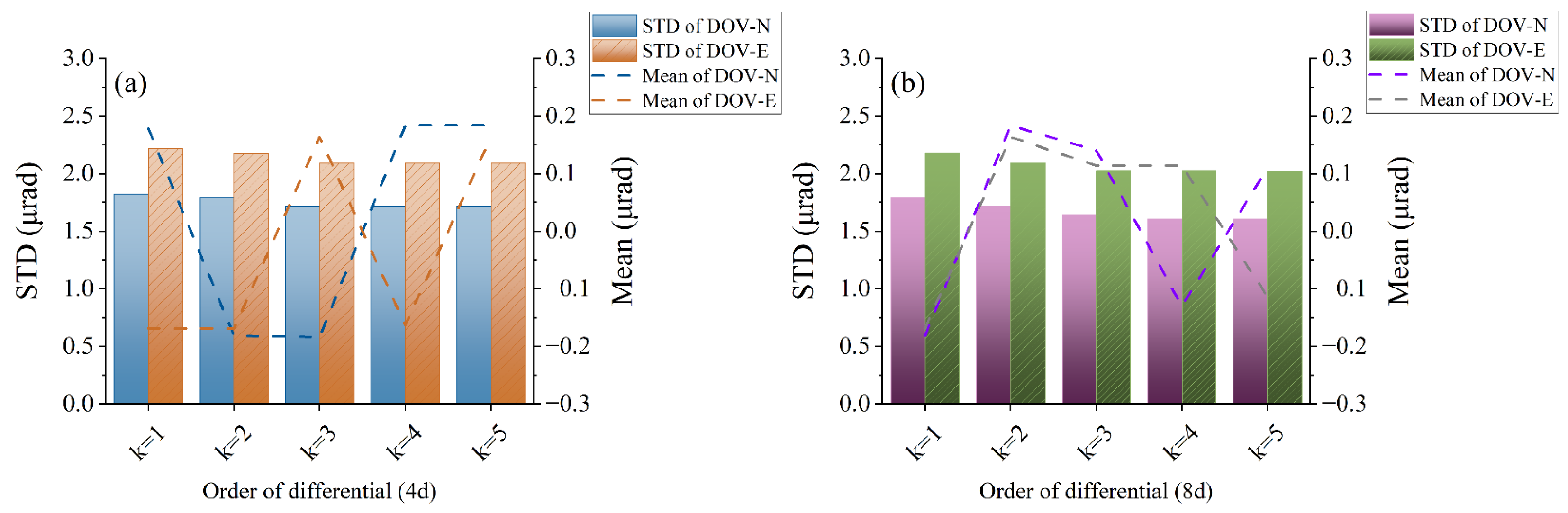
SWOT_DOV is estimated using both 4d and 8d direction data strategies, and the results are obtained by weighted stacking. The resulting SWOT_DOV is compared with SIO east_32.1 and north_32.1. The corresponding differences are shown in Figure 5.

As shown in Figure 5, the inclusion of data from the two diagonal directions significantly improves the results compared with those of 4d. The red horizontal line in the figure represents the best result of the north component in Figure 5a (N = 5, STD = 1.71 μrad), which is used as the reference level. Nevertheless, a noticeable difference still exists between the north and east components. The results of 8d remain stable when the fifth-order neighboring grid points around the central node are used for discretization. More tests with higher orders (N = 10, 20, and 50) show negligible differences compared to N = 5, indicating that the solution is already stable at N = 5. The optimal result yields an accuracy of approximately 0.11 ± 1.60 μrad for the north component and −0.11 ± 2.02 μrad for the east component. In contrast, for the 4d discretization, the optimal results are about 0.18 ± 1.71 μrad for the north component and 0.16 ± 2.09 μrad for the east component.

It is worth noting that, compared with the results obtained by Guo & Wan [15], which used the LSC method, the north component derived from the 4d scheme is comparable to the north_32.1, while improving in the east component. The 8d scheme further enhances the performance, reducing the STD by 0.11 μrad for the north component and 0.22 μrad for the east component, indicating an improvement in accuracy compared with Guo & Wan [15], under the same data and validation framework. These results demonstrate that the ODM is reliable and capable of deriving high-precision DOV from SWOT/KaRIn data with an accuracy of about 1.60 μrad (north) and 2.02 μrad (east). Taking the 8d scheme (N = 5) as an example, the spatial distribution of the signals and the validation results against the SIO model are presented in Figure 6.

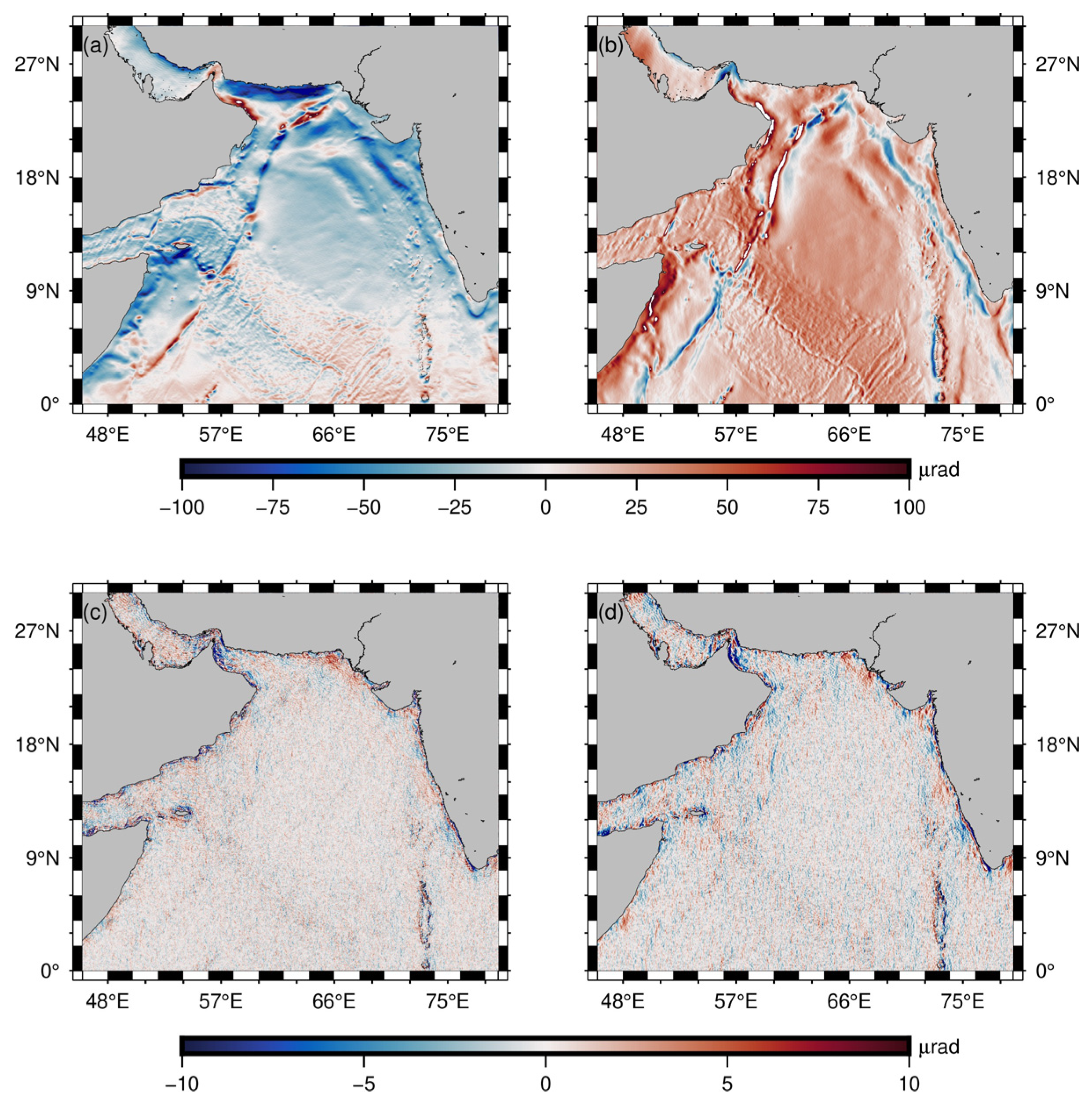
As shown in Figure 6, outlier differences between SWOT_DOV and the SIO DOV models are mainly observed in the coastal regions. The ODM may lead to data gaps near the boundaries of the study area. This issue becomes more evident when higher-order differencing is applied. To avoid missing results near the coast, the geoid from the EGM2008 model is used to fill the inland coastal grid points before performing the discretization. This ensures spatial continuity of the final results. It can also be observed that the validation residuals of the east component are larger and more widely distributed along the coast compared with those of the north component. Overall, relying solely on SWOT data is still insufficient to achieve a balance in the accuracy of the two components of DOV in a local region. The results of the east component can be attributed to the orbital inclination and the relatively lower availability of across-track information.

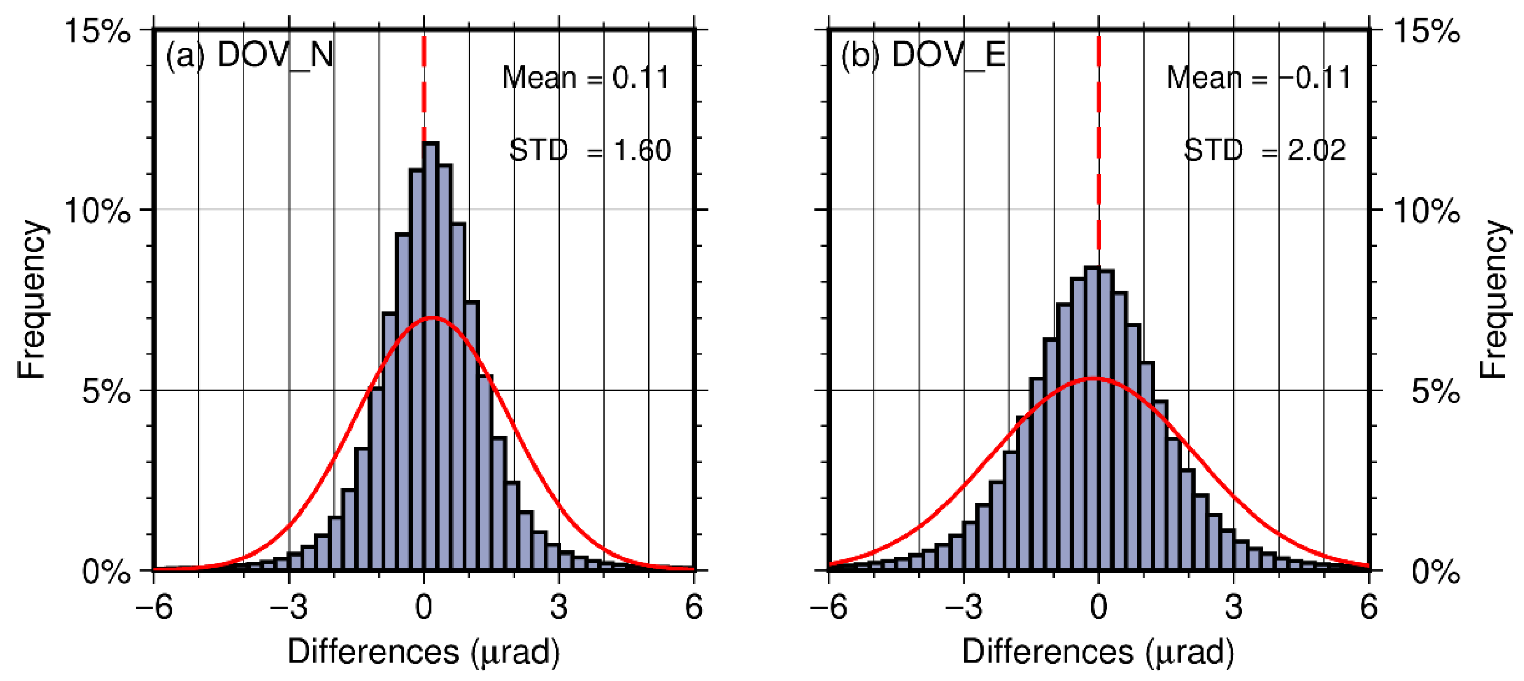
Detailed statistical results are presented in

Table 2. Statistics of validation (unit: urad).

Item	Min	Max	Mean	STD	RMS	MAE
SWOT_DOV_N	−177.35	156.92	−12.17	21.41	24.63	15.29
SWOT_DOV_E	−157.54	227.29	19.83	21.74	29.42	15.05
reDOV_N	−2.31	2.32	0.02	0.23	0.23	0.13
reDOV_E	−1.94	1.96	0.04	0.22	0.22	0.13
SWOT_DOV_N vs. north_32.1	−31.68	45.21	0.11	1.60	1.60	0.97
SWOT_DOV_E vs. east_32.1	−53.66	43.41	−0.11	2.02	2.02	1.23

, including signals of SWOT_DOV, signals of residual SWOT_DOV (reDOV), and differences between SWOT_DOV and SIO DOV. The histograms of the residuals for the two components are shown in Figure 7.

The statistics of the reDOV show that the dispersion of the two components is consistent. This is particularly evident in the MAE values, which are less sensitive to outliers and, therefore, better reflect the overall error level. The last two rows list the residual statistics obtained from the comparison with the SIO model. The mean differences are 0.11 μrad for the north component and −0.11 μrad for the east component, both close to zero, indicating that the ODM is reliable. Compared with the results reported in Guo & Wan, the present results show a slight improvement [15].

The histogram range in Figure 7 is consistent with that used in Guo & Wan [15], and the bin width is set to 0.3 μrad. The comparison shows a distinctive feature of the ODM, that the differences with the SIO model are relatively evenly distributed. The distributions of the bins indicate that no significant systematic bias is present.

The STDs are 1.60 μrad and 2.02 μrad for the north and east components, respectively. The residuals generally follow a Gaussian distribution. The datasets used in this study are the same as those in Guo & Wan [15], the only difference lies in the method used to compute DOV. Therefore, the statistics of the validation results can be directly compared. The results show that the ODM performs slightly better than the LSC method, including 6.4% for the north component and 10.2% for the east component.

4.2. Results of SWOT_GA

4.2.1. Validations of SWOT_GA by Shipborne Gravity Data and Marine GA Models

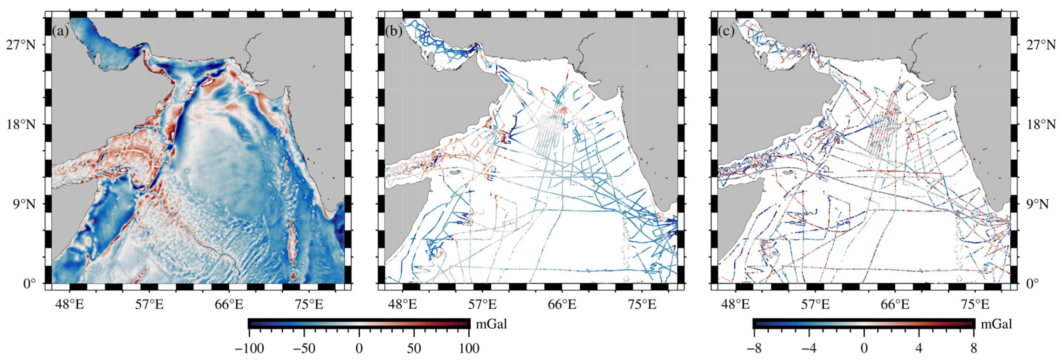
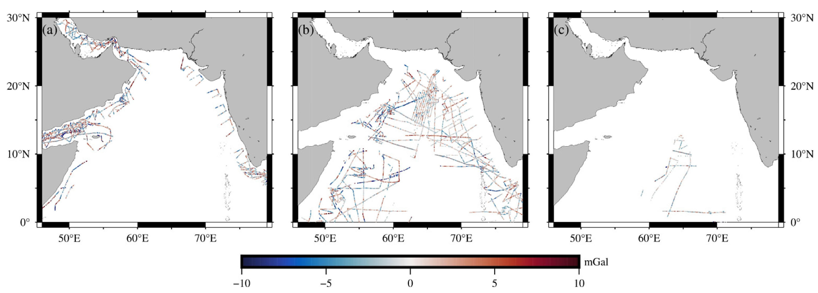
Real observations of the marine DOV are not available in the Arabian Sea. Therefore, the accuracy of SWOT_DOV cannot be validated directly. Instead, the reliability of the method can be assessed indirectly through the accuracy of the derived SWOT_GA. Based on the SWOT_DOV derived using the ODM, SWOT_GAs are computed using the IVM formula. The results are validated using NCEI shipborne gravity data and high-precision external GA models. The spatial distribution of SWOT_GA, the locations of the NCEI shipborne gravity data, and the residuals between SWOT_GA and the NCEI data are shown in Figure 8.

Figure 8b shows the distribution of the processed NCEI shipborne gravity data, including a total of 34 cruises. Using the EGM2008 gravity model as a reference, outliers are removed, and the systematic errors, including gravity datum offsets and instrumental drift, are corrected using a second-order polynomial function. Three cruises, ch043l02, shack375, and shack475, are entirely removed because their data quality did not meet the required standards based on a 3σ threshold relative to the EGM2008 reference field. In total, 103,927 points from the NCEI dataset are used to validate SWOT_GA and the other GA models.

The residual statistics between the NCEI data and each model are summarized in

Table 3. The statistics of validation (unit: mGal).

Validations	Min	Max	Mean	STD	MAE
grav_32.1 vs. NCEI	−36.57	31.88	−0.04	3.92	2.83
grav_SWOT_04 vs. NCEI	−24.62	31.09	−0.09	3.63	2.66
DTU21GRA vs. NCEI	−26.17	27.95	−0.01	3.70	2.76
SDUST2022GRA vs. NCEI	−23.68	27.55	−0.12	3.70	2.75
GMGA2 vs. NCEI	−21.74	29.79	−0.14	4.25	3.15
SWOT_GA (N = 1) vs. NCEI	−20.22	27.37	0.11	3.97	2.98
SWOT_GA (N = 5) vs. NCEI	−21.43	29.35	0.11	3.85	2.84
SWOT_GA (N = 1) vs. grav_32.1	−91.55	78.65	−0.13	2.85	1.80
SWOT_GA (N = 1) vs. grav_SWOT_04	−84.75	51.87	−0.17	2.85	1.85
SWOT_GA (N = 1) vs. DTU21GRA	−65.65	48.52	−0.05	2.35	1.58
SWOT_GA (N = 1) vs. SDUST2022GRA	−97.97	82.37	0.15	2.81	1.77
SWOT_GA (N = 1) vs. GMGA2	−48.97	45.74	−0.32	3.24	2.71
SWOT_GA (N = 5) vs. grav_32.1	−97.97	82.37	0.11	2.75	1.74
SWOT_GA (N = 5) vs. grav_SWOT_04	−85.43	50.59	−0.04	2.68	1.69
SWOT_GA (N = 5) vs. DTU21GRA	−64.04	47.43	0.07	2.20	1.49
SWOT_GA (N = 5) vs. SDUST2022GRA	−41.21	81.16	0.03	2.50	1.56
SWOT_GA (N = 5) vs. GMGA2	−52.13	68.72	−0.14	3.09	2.26

. The table also includes the differences between SWOT_GA and the other GA models. SWOT_GA is derived from two parts: one with 4d-data and N = 1 (shortly named SWOT_GA (N = 1) in Table 3), and the other with 8d-data and N = 5 (SWOT_GA (N = 5)). The former’s scheme is similar to that used by Sandwell et al. [18] and Yu et al. [35]. The latter considers contributions from multiple directions and grid points. Validations of these results assess the performance of the ODM.

Compare the validation results of SWOT_GA (N = 1) and SWOT_GA (N = 5), highlighting the advantage of the proposed ODM. Validated by NCEI shipborne data, the STD decreases from 3.97 to 3.85 mGal, indicating an obvious improvement in accuracy. Similar improvements are observed in the comparisons with existing GA models. The STD of differences with DTU21GRA drops from 2.35 to 2.20 mGal. The STD with grav_32.1 decreases from 2.85 to 2.75 mGal. The agreement with grav_SWOT_04 also improves, with the STD reduced from 2.85 to 2.68 mGal.

The following statistics are based on the SWOT_GA results derived from 8d-data and N = 5. The results show that the mean of differences between all models and the NCEI shipborne gravity data are close to zero, indicating that there is no significant systematic bias. The STD of the residuals between SWOT_GA and the NCEI data is 3.85 mGal. This value is comparable to those of several high-precision global marine GA models, including grav_32.1 (3.92 mGal), grav_SWOT_04 (3.63 mGal), DTU21GRA (3.70 mGal), and SDUST2022GRA (3.70 mGal). From the comparison of grav_32.1 and grav_SWOT_04 with the NCEI data, the inclusion of SWOT/KaRIn data further improves the accuracy of the GA model. Based on validation against NCEI shipborne gravity data, the STD is 3.93 mGal reported in Guo & Wan, where the SWOT_GA in this study shows an improved accuracy by 0.08 mGal [15], which is an improvement of about 2.0%. These results suggest that SWOT_GA achieves a high level of accuracy in the Arabian Sea comparable to that provided by Guo & Wan [15].

The differences between SWOT_GA and the GA models show STDs ranging from 2.20 to 3.09 mGal. Among them, the best consistency is achieved with DTU21GRA (STD = 2.20 mGal), representing an improvement of 0.07 mGal compared to the results of Guo & Wan [15]. The SWOT_GA also shows improved agreement with grav_32.1, with the STD reduced by 0.05 mGal. The differences between SWOT_GA and grav_SWOT_04 are smaller than those with grav_32.1. This is because both models contain SWOT/KaRIn signals. The STD of the differences is 2.68 mGal. Overall, the SWOT_GA model derived from SWOT/KaRIn data demonstrates a high level of consistency with existing models, with STD of differences ranging from 2.20 to 3.09 mGal. This also reflects the reliability of the SWOT_DOV estimated by the ODM.

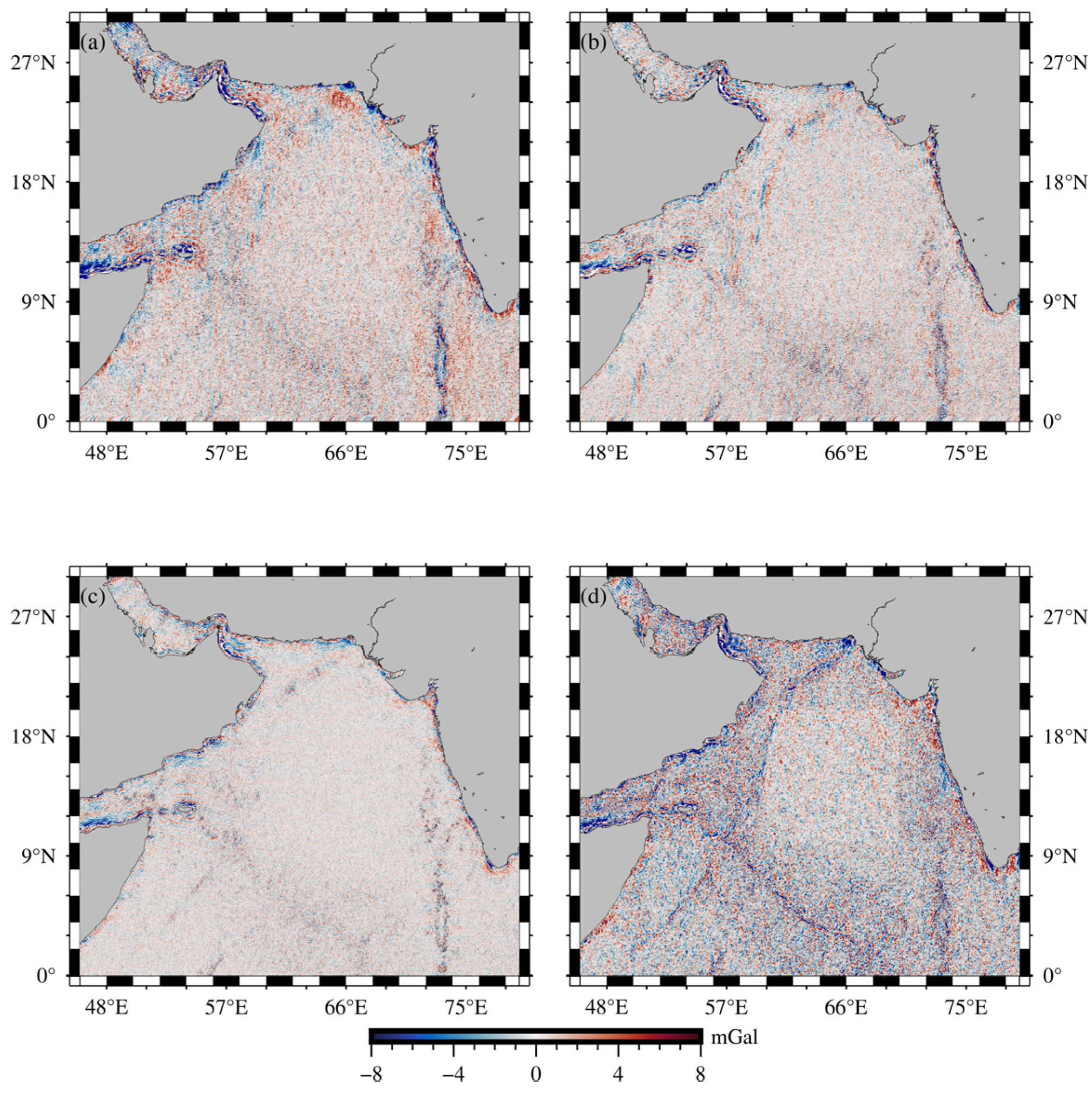
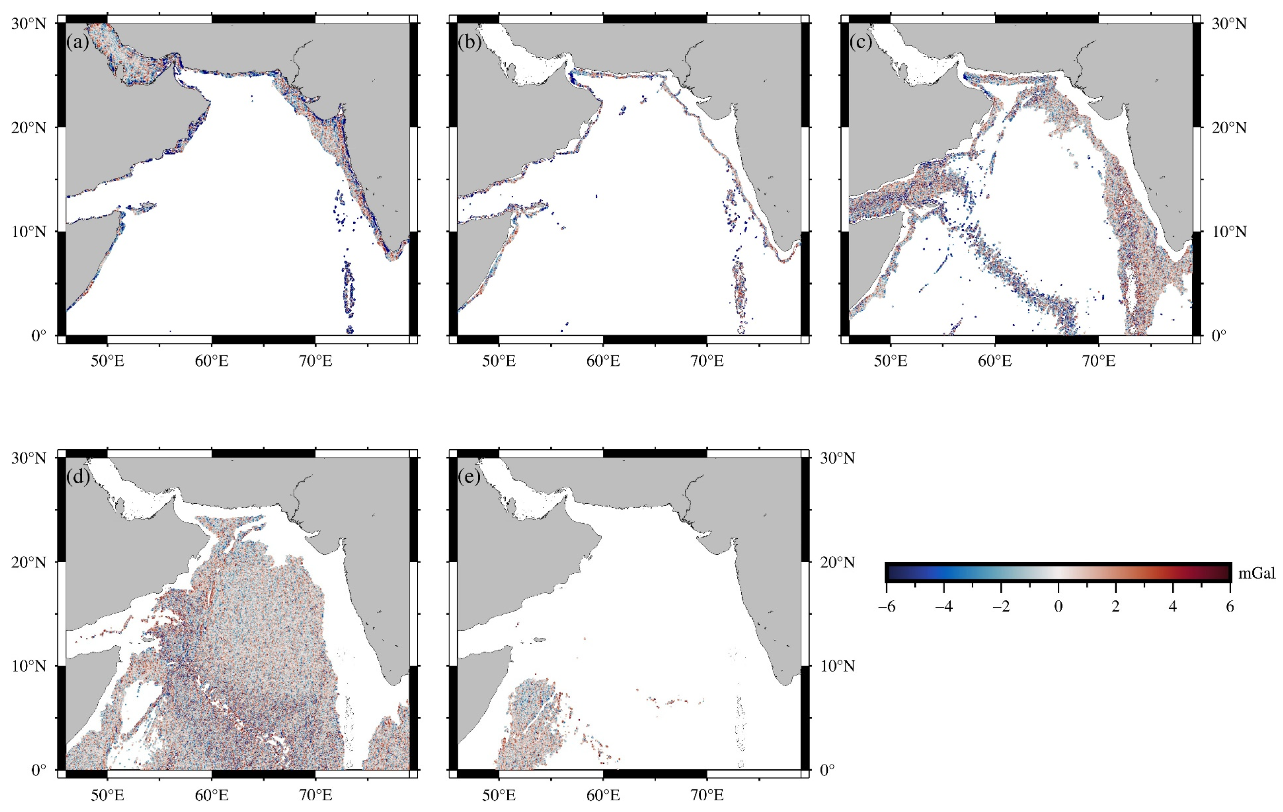
Figure 9 shows the differences between SWOT_GA and four high-precision global marine GA models. Larger residuals occur mainly in coastal regions and along continental margins. These discrepancies are largely related to the complex coastal topography and land–sea transition noises. In contrast, the differences in the open ocean are generally small and evenly distributed, broadly consistent with those GA models. The largely random distribution of the residuals also demonstrates that multi-cycle stacking of SWOT/KaRIn data, combined with the ODM, effectively suppresses noise and stripe errors. As a result, SWOT_GA remains stable.

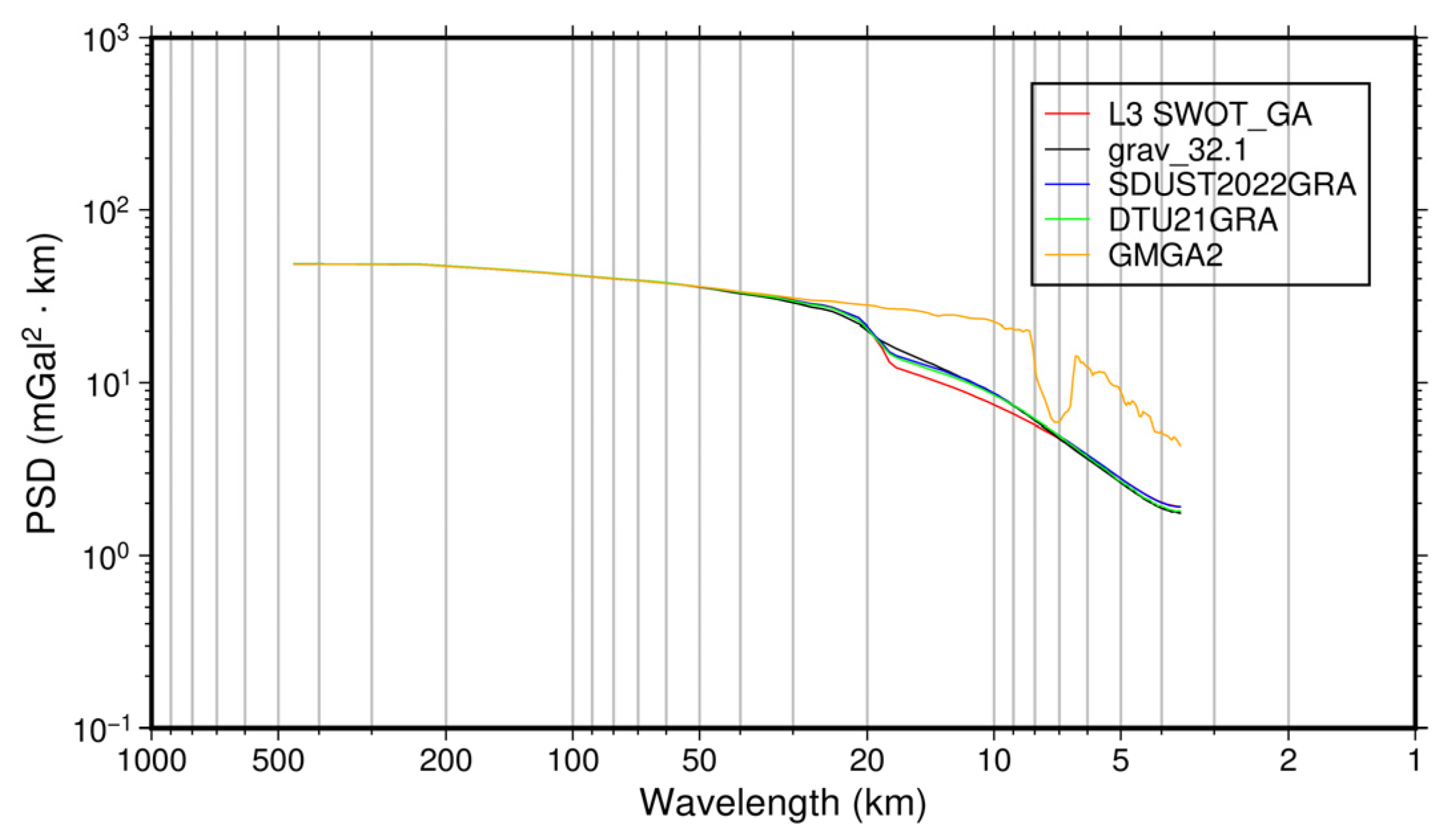
SWOT_GA agrees well with both DTU21GRA and SDUST2022GRA. This suggests that the short-wavelength gravity signals are well captured. In contrast, the discrepancies with GMGA2 are more obvious, mainly related to differences in the data sources and processing strategies. Plot the power spectral density (PSD) between all these GA models in Figure 10.

The PSD shows that SWOT_GA is consistent with existing high-resolution models at long wavelengths and intermediate scales. At short wavelengths, a gradual attenuation is observed in SWOT_GA, whereas GMGA2 exhibits higher spectral power due to the inclusion of bathymetry forward modeling. Figure 10 suggests that SWOT_GA achieves a good balance between signal recovery and noise suppression, ensuring both accuracy and stability.

Overall, multi-cycle stacking effectively reduces along-track errors. The quality of SWOT_GA is comparable to existing high-precision models. The SWOT_DOV derived by the ODM is, therefore, reliable. These further confirm the strong potential of SWOT wide-swath altimetry for high-resolution marine gravity field recovery.

4.2.2. Impact of Seafloor Topography Gradient and Water Depths on Accuracy of the SWOT_GA

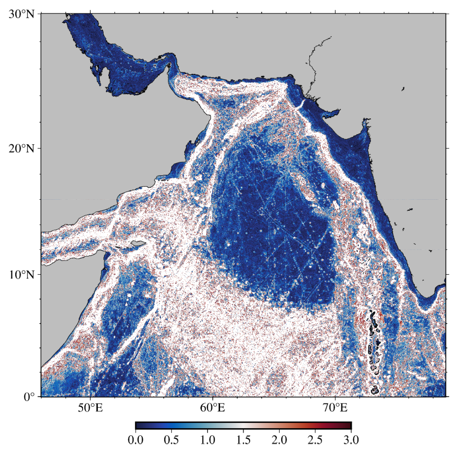
The study area considered in this experiment is characterized by complex seafloor topography. To further investigate the influence of seabed terrain on SWOT_GA, the topography gradient of the study region is calculated using the Topo_27.1 model, as shown in Figure 11.

The residuals obtained from the validation of SWOT_GA using NCEI shipborne gravity data are classified into four groups according to the range of gradients. Based on this classification, the data quality is analyzed separately for different terrain conditions. The corresponding statistical results are presented in

Table 4. Statistics of results validated by NCEI data in different ocean topography (unit: mGal).

Slope Range (%)	Points	Min	Max	Mean	STD	MAE
<1	52,267	−21.72	30.70	−0.20	3.43	2.58
1~2	16,028	−19.80	23.77	−0.26	3.92	3.00
2~3	8747	−21.18	21.98	−0.42	4.41	3.40
>3	26,885	−21.43	29.35	0.17	5.15	3.94

.

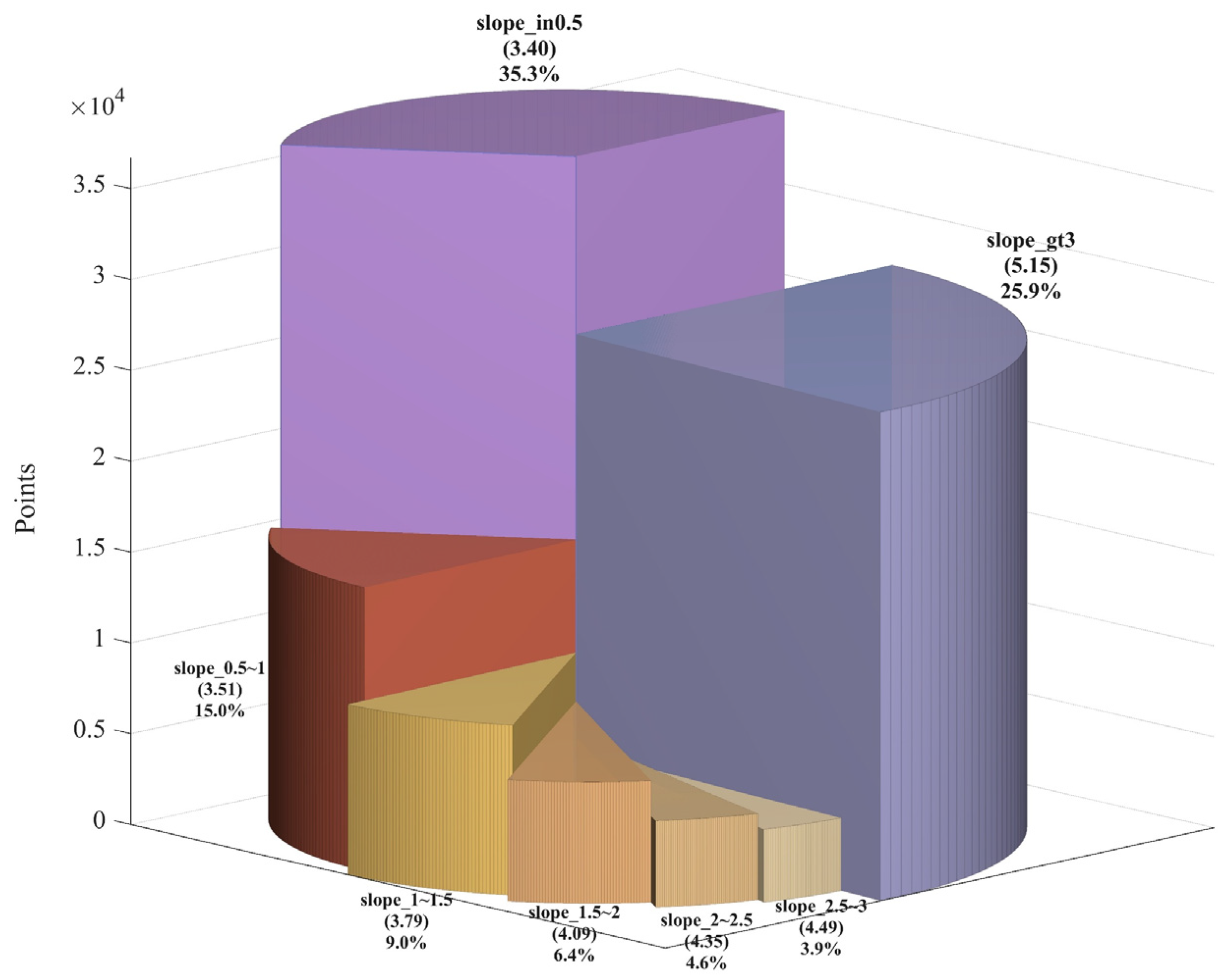
Residual data located in regions with a gradient of less than 1% account for 50.3% of the total. In contrast, areas with gradients between 2% and 3% contain the smallest proportion of data of only 8.4%. Regions with gradients between 1% and 2% represent 15.4%, while those with gradients greater than 3% account for 25.9%. These results indicate that observations located in regions with terrain gradients below 1% largely determine the overall data quality of SWOT_GA across the Arabian Sea. To examine this relationship in more detail, the topography gradients are further subdivided, and the data quality within each range is analyzed. The results are presented using a Nightingale rose chart, as shown in Figure 12.

In this chart, each sector represents a specific range of topography gradients. The height of each sector indicates the number of validation points located within that range. The size of the sector reflects the STD of the residuals in the corresponding interval. The detailed statistics shown in this figure are consistent with the conclusions presented in Table 4. The validation results of SWOT_GA against the NCEI shipborne gravity data are mainly controlled by regions with relatively small topography gradients. In particular, areas with slopes below 0.5% account for 35.3% of the total data, and the STD of the validation residuals in these regions is only 3.4 mGal.

However, regions with slopes greater than 3% still represent 25.9% of the study area. This indicates that a substantial portion of the region is characterized by strong topographic variations. Such areas usually correspond to seamounts, mid-ocean ridges, fracture zones, and continental slopes, as highlighted by the red regions in Figure 11. Overall, these results demonstrate that SWOT/KaRIn data is capable of recovering the GA model even in regions with complex seafloor topography. This capability is supported by both the validation against NCEI shipborne gravity data and the comparisons with external high-precision GA models.

Using the bathymetric data provided by Topo_27.1, the distribution and quality of SWOT_GA relative to grav_32.1 are analyzed across different depth ranges, as shown in Figure 13. In addition, the differences between SWOT_GA and shipborne gravity data are examined at different distances from the coastline, with the results presented in Figure 14.

Figure 13 shows that the differences between SWOT_GA and grav_32.1 are relatively large in near-coast regions, while the discrepancies gradually decrease as depth increases. In coastal and continental shelf areas, the signals are strongly influenced by coastal topography, which leads to larger differences. In these regions, the STD is about 5.3 mGal. Although the statistical results in the ranges shown in Figure 13a,b appear relatively poor, the number of data points in these areas is limited, accounting for only 10.3% and 2.9% of the total points, respectively.

In contrast, in deep-ocean regions (>3000 m), the range of the residuals becomes significantly smaller. As shown in Figure 13d,e, the STD values are 1.55 mGal and 1.31 mGal, respectively. The number of points within these two depth ranges accounts for 59.8% and 5.4% of the total observations. In fact, once the depth exceeds 1000 m, the differences between SWOT_GA and grav_32.1 decrease markedly. For example, the STD in the depth range shown in Figure 13b is 5.41 mGal, whereas it decreases to 2.48 mGal in the range shown in Figure 13c. Data within this depth range contribute 21.7% of the total observations in the study area.

Within 0–50 km from the coastline, the differences between SWOT_GA and the gravity data are most pronounced, with an STD of 4.56 mGal. The number of points in this range accounts for about 34.5% of the total. As the distance from the coast increases to 50–200 km, the discrepancies decrease markedly, and the STD drops to approximately 3.45 mGal. Data in this range represent about 62.2% of the observations.

When the distance from the coast exceeds 200 km, the STD stabilizes at around 3.15 mGal. Notably, the data points located between 200 and 1000 km only contribute 3.3% of the total. The results shown in Figure 13 and Figure 14 indicate that SWOT wide-swath data can reliably restore high-precision marine GA in the open ocean. In contrast, the accuracy in near-coastal regions is still constrained by observation conditions and the complexity of the coastal environment.

5. Discussion

Multiple comparative experiments confirm the reliability of the ODM proposed in this study. The method can produce stable SWOT_DOV and, subsequently, derive high-accuracy SWOT_GA. However, computational efficiency is also an important factor that must be considered. The computation time is, therefore, recorded during the experiments, and the results are summarized in

Table 5. Statistics on the time consumption of the two methods.

Item	Time (s)	Computing Platform
LSC	~900	AMD Ryzen 9 7945HX (2.50 GHz)
ODM	~108

.

The computation of SWOT_DOV is performed automatically from first-order to fifth-order differencing, and the results are output at each step. The reported time represents the average runtime, including the time required to write the results to files. The runtime for reproducing the LSC method is approximately 15 min (about 900 s). In comparison, the ODM requires about 1.8 min (approximately 108 s) on average. All experiments are carried out on an AMD Ryzen 9 7945HX platform. The computation time may vary slightly between runs, as it depends on the processor and memory conditions during execution.

In general, the LSC method requires a sliding-window procedure to grid the data, which is computationally intensive. In contrast, the ODM performs the gridding using the GMT, while the subsequent processing steps are implemented using a vectorized workflow. As a result, the computational efficiency of the ODM is significantly higher.

6. Conclusions

In this study, the ODM is proposed to construct a 1′ gridded SWOT_DOV based on SWOT/KaRIn L2 data in the Arabian Sea and its surrounding regions. The accuracy of SWOT_DOV is evaluated using the widely recognized SIO V32.1 model. The STD of the differences is 1.60 μrad for the north component and 2.02 μrad for the east component, which is compared with those calculated by the LSC method. The results indicate that the SWOT_DOV derived using the ODM shows a spatial pattern more consistent with the SIO model than that derived from the LSC method.

Based on the estimated SWOT_DOV, 1′ grid SWOT_GA is further derived using the IVM formula. The accuracy of SWOT_GA is validated using NCEI shipborne gravity data and four external high-precision marine GA models. Validation against the NCEI shipborne gravity data yields a residual STD of 3.85 mGal. This level of accuracy is comparable to that of internationally recognized high-precision models, including grav_32.1 (3.92 mGal), grav_SWOT_04 (3.63 mGal), DTU21GRA (3.70 mGal), and SDUST2022GRA (3.70 mGal). SWOT_GA shows the best agreement with DTU21GRA, with an STD of 2.20 mGal. It reflects the quality of the estimated SWOT_DOV and confirms the reliability of the ODM.

Analysis of SWOT_GA accuracy under different seafloor topography gradients shows that most residuals are located in regions with relatively gentle topography. Combined analyses based on depth ranges and distance from the coastline further indicate that deep-ocean and offshore regions contribute the majority of stable and high-quality gravity information in the study area. These findings demonstrate that SWOT/KaRIn data have a strong capability to recover high-precision marine gravity field features in open-ocean environments.

References

1. Yuan, J.; Guo, J.; Liu, X.; Zhu, C.; Niu, Y.; Li, Z.; Ji, B.; Ouyang, Y. Mean sea surface model over China seas and its adjacent ocean established with the 19-year moving average method from multi-satellite altimeter data. Cont. Shelf Res. 2020, 192, 104009. [Google Scholar] [CrossRef]
2. Andersen, O.B.; Knudsen, P.; Berry, P.A.M. The DNSC08GRA global marine gravity field from double retracked satellite altimetry. J. Geod. 2010, 84, 191–199. [Google Scholar] [CrossRef]
3. Guo, J.Y.; Qin, J.; Kong, Q.L.; Li, G.-W. On simulation of precise orbit determination of HY-2 with centimeter precision based on satellite-borne GPS technique. Appl. Geophys. 2012, 9, 95–107. [Google Scholar] [CrossRef]
4. Hwang, C.; Tseng, T.-P.; Lin, T.-J.; Švehla, D.; Hugentobler, U.; Chao, B.F. Quality assessment of FORMOSAT-3/COSMIC and GRACE GPS observables: Analysis of multipath, ionospheric delay and phase residual in orbit determination. GPS Solut. 2010, 14, 121–131. [Google Scholar] [CrossRef]
5. Ji, H.; Guo, J.; Zhu, C.; Yuan, J.; Liu, X.; Li, G. On Deflections of Vertical Determined From HY-2A/GM Altimetry Data in the Bay of Bengal. IEEE J. Sel. Top. Appl. Earth Obs. Remote Sens. 2021, 14, 12048–12060. [Google Scholar] [CrossRef]
6. Ji, H.; Liu, X.; Zhu, C.; Yuan, J.; Ji, B.; Guo, J. On performance of CryoSat-2 altimeter data in deriving marine gravity over the Bay of Bengal. Mar. Geophys. Res. 2021, 42, 39. [Google Scholar] [CrossRef]
7. Zhu, C.; Guo, J.; Gao, J.; Liu, X.; Hwang, C.; Yu, S.; Yuan, J.; Ji, B.; Guan, B. Marine gravity determined from multi-satellite GM/ERM altimeter data over the South China Sea: SCSGA V1.0. J. Geod. 2020, 94, 50. [Google Scholar] [CrossRef]
8. Li, J.C.; Chen, J.Y.; Ning, J.S.; Chao, D.B. Approximation Theory of the Earth Gravity Field and Determination of the Chinese Gravity Geoid Model 2000; Wuhan University Press: Wuhan, China, 2003. [Google Scholar]
9. Li, Z.; Guo, J.Y.; Ji, B.; Wan, X.Y.; Zhang, S.J. A review of marine gravity field recovery from satellite altimetry. Remote Sens. 2022, 14, 4790. [Google Scholar] [CrossRef]
10. Li, Z.; Guo, J.Y.; Zhu, C.C.; Liu, X.; Hwang, C.; Lebedev, S.; Chang, X.; Soloviev, A.; Sun, H. The SDUST2022GRA global marine gravity anomalies recovered from radar and laser altimeter data: Contribution of ICESat-2 laser altimetry. Earth Syst. Sci. Data 2024, 16, 4119–4135. [Google Scholar] [CrossRef]
11. Wan, X.Y.; Wang, F.; Guo, H.Y.; Liu, B. Impact of Errors in Environmental Correction on Gravity Field Recovery Using Interferometric Radar Altimeter Observations. Remote Sens. 2022, 14, 6299. [Google Scholar] [CrossRef]
12. Zhu, C.C.; Liu, X.; Guo, J.Y.; Yu, S.; Niu, Y.; Yuan, J.; Li, Z. Sea Surface Heights and Marine Gravity Determined from SARAL/AltiKa Kaband Altimeter Over South China Sea. Pure Appl. Geophys. 2021, 178, 1513–1527. [Google Scholar] [CrossRef]
13. Bao, L.F.; Xu, H.Z.; Li, Z.C. Towards a 1 mGal accuracy and 1 min resolution altimetry gravity field. J. Geod. 2013, 87, 961–969. [Google Scholar] [CrossRef]
14. Guo, H.Y.; Wan, X.Y.; Wang, H.B. Validation of just-released SWOTL2KaRInbeta pre-validated data based on restore the marine gravity field and its application. IEEE J. Sel. Top. Appl. Earth Obs. Remote Sens. 2024, 17, 7878–7887. [Google Scholar] [CrossRef]
15. Guo, H.Y.; Wan, X.Y. Deriving full-tensor gravity gradients over the Arabian Sea from SWOT altimetry using a stacked discretization method. Adv. Space Res. 2026, 77, 5717–5736. [Google Scholar] [CrossRef]
16. Jin, T.; Zhou, M.; Zhang, H.; Li, J.; Jiang, W.; Zhang, S.; Hu, M. Analysis of vertical deflections determined from one cycle of simulated SWOT wide-swath altimeter data. J. Geod. 2022, 96, 30. [Google Scholar] [CrossRef]
17. Li, Y.; Zhou, J.; Li, J.; Li, N.; Zhu, F.; Sun, H. Global marine gravity from 27 cycles of SWOT satellite data: Accuracy and spatial resolution evaluation. J. Geod. 2025, 99, 51. [Google Scholar] [CrossRef]
18. Sandwell, D.T.; Muller, R.D.; Smith, W.H.F. New global marine gravity model from CryoSat-2 and Jason-1 reveals buried tectonic structure. Science 2014, 346, 65–67. [Google Scholar] [CrossRef] [PubMed]
19. Sun, M.; Feng, W.; An, D.; Chen, X.; Yang, M.; Zhong, M. Preliminary Results of Marine Gravity Anomaly and Bathymetry From SWOT Wide-Swath Altimeter Data. IEEE J. Sel. Top. Appl. Earth Obs. Remote Sens. 2025, 18, 18107–18116. [Google Scholar] [CrossRef]
20. Yuan, J.J.; Guo, J.Y.; Zhu, C.C.; Li, Z.; Liu, X.; Gao, J.Y. SDUST2020 MSS: A global 1′× 1′ mean sea surface model determined from multi-satellite altimetry data. Earth Syst. Sci. Data Discuss. 2022, 15, 155–169. [Google Scholar] [CrossRef]
21. Zhu, C.; Guo, J.; Ya, S.; Li, W.; Gao, J.; Qiu, L. Moving Geoid Gradient Method for High-Precision and High-Resolution Gravity Recovery From SWOT Wide-Swath Data. IEEE Trans. Geosci. Remote Sens. 2025, 63, 1–13. [Google Scholar] [CrossRef]
22. Yang, J.J.; Jekeli, C.; Liu, L.T. Seafloor topography estimation from gravity gradients using simulated annealing. J. Geophys. Res. Solid Earth 2018, 123, 6958–6975. [Google Scholar] [CrossRef]
23. Annan, R.F.; Wan, X.Y. Recovering Bathymetry of the Gulf of Guinea Using Altimetry-Derived Gravity Field Products Combined via Convolutional Neural Network. Surv. Geophys. 2022, 43, 1541–1561. [Google Scholar] [CrossRef]
24. Guo, H.; Wan, X.; Wang, F.; Tian, S. Expected precision of gravity gradient recovered from Ka-Band radar interferometer observations and impact of instrument errors. Remote Sens. 2024, 16, 576. [Google Scholar] [CrossRef]
25. Wan, X.Y.; Ran, J.J.; Jin, S.G. Sensitivity analysis of gravity anomalies and vertical gravity gradient data for bathymetry inversion. Mar. Geophys. Res. 2018, 40, 87–96. [Google Scholar] [CrossRef]
26. Wan, X.Y.; Wang, H.B.; Jia, Y.J. Performance of Haiyang-2 Derived Gravity Field Products in Bathymetry Inversion. Remote Sens. 2023, 15, 32. [Google Scholar] [CrossRef]
27. Wan, X.Y.; Annan, R.F.; Yao, Z. Altimetry-derived Gravity Gradients using Spectral Method and Their Performance in Bathymetry Inversion using Back-Propagation Neural Network. J. Geophys. Res. Solid Earth 2023, 128, e2022JB025785. [Google Scholar] [CrossRef]
28. Wan, X.Y.; Zhang, L.J.; Guo, H.Y.; Annan, R.F. Bathymetry Inversion Using Full Tensor Gravity Gradients: A Case Study in the Bay of Bengal. IEEE J. Sel. Top. Appl. Earth Obs. Remote Sens. 2026, 19, 8071–8079. [Google Scholar] [CrossRef]
29. Fu, L.L.; Ubelmann, C. On the transition from profile altimeter to swath altimeter for observing global ocean surface topography. J. Atmos. Ocean. Technol. 2014, 31, 560–568. [Google Scholar] [CrossRef]
30. Fu, L.L.; Chao, Y.; Laignel, B.; Turki, I., Sr. Mapping coastal sea level at high resolution with radar interferometry: The SWOT Mission. In Proceedings of the 2017 Fall Meeting, AGU, New Orleans, LA, USA, 11–15 December 2017. [Google Scholar]
31. Hwang, C.; Yu, D.C. Transforming coastal mapping from space. Science 2024, 386, 1222–1223. [Google Scholar] [CrossRef]
32. Guo, H.Y.; Wan, X.Y.; Zhang, K.Y.; Jia, Y.J.; Ran, J.J. An improved latitude difference method for SWOT accuracy evaluation using crossover discrepancies. IEEE Trans. Geosci. Remote Sens. 2025, 63, 4203912. [Google Scholar] [CrossRef]
33. Wan, X.; Jin, S.; Liu, B.; Tian, S.; Kong, W.; Annan, R.F. Effects of InSAR Altimetry Errors on Marine Gravity Field Inversion. Sensors 2020, 20, 2465. [Google Scholar] [CrossRef]
34. Yu, D.; Hwang, C.; Andersen, O.B.; Chang, E.T.; Gaultier, L. Gravity recovery from SWOT altimetry using geoid height and geoid gradient. Remote Sens. Environ. 2021, 265, 112650. [Google Scholar] [CrossRef]
35. Yu, Y.; Sandwell, D.T.; Dibarboure, G. Abyssal marine tectonics from the SWOT mission. Science 2024, 386, 1251–1256. [Google Scholar] [CrossRef]
36. Yu, Y.; Sandwell, D.T.; Dibarboure, G.; Chen, C.; Wang, J. Accuracy and resolution of SWOT altimetry: Foundation seamounts. Earth Space Sci. 2024, 11, e2024EA003581. [Google Scholar] [CrossRef]
37. Sun, M.Z.; Feng, W.; Yu, D.C.; Chen, X.D.; Liang, W.X.; Zhong, M. Analysing the impact of SWOT observation errors on marine gravity recovery. Geophys. J. Int. 2024, 237, 862–871. [Google Scholar] [CrossRef]
38. Hay, A.; Watson, C.; Legresy, B.; King, M.; Zhou, B.; Beardsley, J.; Bohé, A. In situ geometric validation of SWOT satellite observations in Bass Strait, Australia. Earth Space Sci. 2025, 12, e2025EA004326. [Google Scholar] [CrossRef]
39. Zhu, F.; Li, J.; Li, Y.; Xu, J.; Guo, J.; Zhou, J.; Sun, H. Estimating Seafloor Topography of the South China Sea Using SWOT Wide-Swath Altimetry Data. IEEE J. Sel. Top. Appl. Earth Obs. Remote Sens. 2025, 18, 3569–3580. [Google Scholar] [CrossRef]
40. Ya, S.; Liu, X.; Zhou, R.; Li, Z.; Bian, S.; Guo, J. High accuracy vertical gradient of gravity anomaly model determined from SWOT/KaRIn altimetry data during scientific phase. Acta Geod. Cartogr. Sin. 2025, 54, 1583–1595. [Google Scholar] [CrossRef]
41. Li, Z.; Guo, J.; Hwang, C.; Yu, D.; Zhang, H.; Sun, H.; Liu, X. Tailored method for optimizing deflection of the vertical model using multidirectional geoid gradients from SWOT/KaRIn observations. Geophys. J. Int. 2026, 244, ggaf484. [Google Scholar] [CrossRef]
42. Feng, W.; An, D.; Hwang, C.; Sun, M.; Chen, X.; Zhang, Z.; Yang, M.; Zhong, M. SYSU_Topo: A 1-arc-minute global bathymetry from SWOT-derived gravity using thegravity–geological method. Sci. Data 2026, 13, 386. [Google Scholar] [CrossRef] [PubMed]
43. Wang, Y.; Wang, J.; Chen, L. Integrating multi-source altimetry observations for gravity anomaly derivation in the South China Sea. Geod. Geodyn. 2026; in press. [CrossRef]
44. Fournier, M.; Chamot-Rooke, N.; Rodriguez, M.; Huchon, P.; Petit, C.; Beslier, M.; Zaragosi, S. Owenfracture zone: The Arabia–India plate boundary unveiled. Earth Planet. Sci. Lett. 2011, 302, 247–252. [Google Scholar] [CrossRef]
45. Zhou, R.C.; Liu, X.; Li, Z.; Sun, Y.; Yuan, J.J.; Guo, J.Y.; Ardalan, A.A. On performance of vertical gravity gradient determined from CryoSat-2 altimeter data over Arabian Sea. Geophys. J. Int. 2023, 234, 1519–1529. [Google Scholar] [CrossRef]
46. Li, Q.Q.; Bao, L.F.; Shum, C.K. Altimeter-derived marine gravity variation studies the submarine plate tectonic motions. Chin. J. Geophys. 2020, 63, 250–2515. [Google Scholar] [CrossRef]
47. Knudsen, P.; Andersen, O.B.; Maximenko, N.; Hafner, J. The DTUUH22MDT combined mean dynamic topography model. In Proceedings of the 2022 Ocean Surface Topography Science Team Meeting, Venice, Italy, 31 October–4 November 2022. [Google Scholar]
48. Zhou, R.C.; Guo, J.Y.; Ya, S.S.; Sun, H.P.; Liu, X. SDUST2023VGGA: A global ocean vertical gradient of gravity anomaly model determined from multidirectional data from mean sea surface. Earth Syst. Sci. Data Discuss. 2025, 17, 817–836. [Google Scholar] [CrossRef]
49. Pavlis, N.K.; Holmes, S.A.; Kenyon, S.C.; Factor, J.K. The development and evaluation of the Earth Gravitational Model 2008 (EGM2008). J. Geophys. Res. Solid Earth 2012, 117, B04406. [Google Scholar] [CrossRef]
50. Sandwell, D.T.; Smith, W.H.F. Marine gravity anomaly from Geosat and ERS 1 satellite altimetry. J. Geophys. Res. Solid Earth 1997, 102, 10039–10054. [Google Scholar] [CrossRef]
51. Sandwell, D.T.; Harper, H.; Tozer, B.; Smith, W.H.F. Gravity field recovery from geodetic altimeter missions. Adv. Space Res. 2021, 68, 1059–1072. [Google Scholar] [CrossRef]
52. Andersen, O.B.; Knudsen, P. The DTU 21 Global Marine Gravity Field-First Evaluation Ocean Surf Topogr Sci Team Meet. Boulder, Colorado. 2021. Available online: http://ftp.space.dtu.dk/pub/Altimetry/CUNDERLIK (accessed on 1 January 2024).
53. Andersen, O.B.; Zhang, S.; Sandwell, D.T.; Dibarboure, G.; Smith, W.H.F.; Abulaitijiang, A. The unique role of the Jason geodetic missions for high resolution gravity field and meansea surface modelling. Remote Sens. 2021, 13, 646. [Google Scholar] [CrossRef]
54. Bako, M.; Kusche, J. Evaluation and homogenization of a marine gravity database from shipborne and satellite altimetry-derived gravity data over the coastal region of Nigeria. J. Appl. Geod. 2024, 19, 175–189. [Google Scholar] [CrossRef]
55. Hao, R.J.; Wan, X.Y.; Annan, R.F. Enhanced Short-wavelength Marine Gravity Anomaly Using Depth Data. IEEE Trans. Geosci. Remote Sens. 2023, 61, 5903109. [Google Scholar] [CrossRef]
56. Wan, X.Y.; Hao, R.J.; Jia, Y.J.; Wu, X.; Wang, Y.; Feng, L. Global marine gravity anomalies from multi-satellite altimeter data. Earth Plan. Space 2022, 74, 165. [Google Scholar] [CrossRef]
57. Guo, J.Y.; Liu, X.; Chen, Y.N. Local normal height connection across sea with ship-borne gravimetry and GNSS techniques. Mar. Geophys. Res. 2014, 35, 141–148. [Google Scholar] [CrossRef]
58. Hwang, C. Inverse vening meinesz formula and deflection-geoid formula: Applications to the predictions of gravity and geoid over the South China Sea. J. Geod. 1998, 72, 304–312. [Google Scholar] [CrossRef]
59. Hwang, C.; Chang, E.T.Y. Seafloor secrets revealed. Science 2014, 346, 32–33. [Google Scholar] [CrossRef] [PubMed]
60. Tian, S. Analysis of Interferometric Imaging Radar Altimeter Errors on Accuracy of Marine Gravity Field Inversion. Master’s Thesis, China University of Geosciences (Beijing), Beijing, China, 2019. [Google Scholar] [CrossRef]
61. Wessel, P.; Luis, J.F.; Uieda, L.; Scharroo, R.; Wobbe, F.; Smith, W.H.F.; Tian, D. The generic mapping tools version 6. Geochem. Geophys. Geosyst. 2019, 20, 5556–5564. [Google Scholar] [CrossRef]
62. Heiskanen, W.A.; Moritz, H. Physical Geodesy; Freeman WH: San Francisco, CA, USA, 1967. [Google Scholar]
63. Hwang, C.; Parsons, B. Gravity anomalies derived from Seasat, Geosat, ERS-1 and TOPEX/POSEIDON altimetry and ship gravity: A case study over the Reykjanes Ridge. Geophys. J. Int. 1995, 122, 551–568. [Google Scholar] [CrossRef]
64. Wessel, P.; Watts, A.B. On the accuracy of marine gravity measurements. J. Geophys. Res. Solid Earth 1988, 93, 393–413. [Google Scholar] [CrossRef]
Figure 1. Topography of the Arabian Sea.
Remotesensing 18 01360 g001
Figure 2. Local distribution of KaRIn data.
Remotesensing 18 01360 g002
Figure 3. Optimized discretization method flowchart.
Remotesensing 18 01360 g003
Figure 4. Multi-directional data utilization. (a) apply 4d data, (b) apply 8d data.
Remotesensing 18 01360 g004
Figure 5. Validation results from SIO V32.1. (a) Results of 4d, (b) results of 8d.
Remotesensing 18 01360 g005
Figure 6. SWOT_DOV and validation results. (a) SWOT_DOV_N, (b) SWOT_DOV_E, (c) differences between SWOT_DOV_N and north_32.1, (d) differences between SWOT_DOV_E and east_32.1.
Remotesensing 18 01360 g006
Figure 7. Histogram of validation results: (a) differences between SWOT_DOV_N and north_32.1, (b) differences between SWOT_DOV_E and east_32.1.
Remotesensing 18 01360 g007
Figure 8. Results of SWOT_GA. (a) SWOT_GA, (b) NCEI shipborne gravity data, (c) differences between SWOT_GA and NCEI data.
Remotesensing 18 01360 g008
Figure 9. Validations of SWOT_GA by the multi-GA model: (a) differences between SWOT_GA and grav_32.1, (b) differences between SWOT_GA and DTU21GRA, (c) differences between SWOT_GA and SDUST2022GRA, (d) differences between SWOT_GA and GMGA2.
Remotesensing 18 01360 g009
Figure 10. Power spectral density analysis of multi-models.
Remotesensing 18 01360 g010
Figure 11. Seafloor topography gradient based on topo_27.1.
Remotesensing 18 01360 g011
Figure 12. Statistics of results considering topography gradient.
Remotesensing 18 01360 g012
Figure 13. SWOT_GA distribution and quality at different depths: (a) 0~200 m in depth, (b) 200~1000 m in depth, (c) 1000~3000 m in depth, (d) 3000~5000 m in depth, (e) >5000 m in depth.
Remotesensing 18 01360 g013
Figure 14. Differences between SWOT_GA and shipborne gravity data at different offshore distances: (a) 0~50 km offshore, (b) 50~200 km offshore, (c) 200~1000 km offshore.
Remotesensing 18 01360 g014