Article

Explainable Artificial Intelligence for Estimating Surface Deformation in Landslide Areas with Incomplete SAR Data

1
Faculty of Engineering, China University of Geosciences, 388 Lumo Rd., Wuhan 430074, China
2
Water Resources Section, Faculty of Civil Engineering and Geosciences, Delft University of Technology, Stevinweg 1, P.O. Box 5048, 2600 GA Delft, The Netherlands
3
School of Environmental Studies, China University of Geosciences, Wuhan 430074, China
4
Centre for Severe Weather and Climate and Hydro-Geological Hazards, Wuhan 430078, China
5
School of Geography and Information Engineering, China University of Geosciences, Wuhan 430074, China
*
Author to whom correspondence should be addressed.
Remote Sens. 2026, 18(9), 1363; https://doi.org/10.3390/rs18091363
Submission received: 22 March 2026 / Revised: 21 April 2026 / Accepted: 23 April 2026 / Published: 28 April 2026
(This article belongs to the Special Issue Geospatial Artificial Intelligence (GeoAI) in Remote Sensing)

Highlights

What are the main findings?
  • A regional-scale surface deformation estimation framework is proposed to robustly and accurately estimate surface deformation in areas with missing SAR data.
  • An explainable artificial intelligence approach is introduced to quantify the effects of geological factors and anthropogenic engineering factors on surface deformation.
What are the implications of the main findings?
  • The proposed framework provides an effective solution for deformation estimation in regions where SAR observations are incomplete, thereby improving the applicability of remote sensing in complex real-world settings.
  • The comparative analysis of different ensemble learning models offers useful guidance for selecting suitable models for regional surface deformation estimation.

Abstract

In landslide-prone areas, spatial gaps in InSAR-derived deformation maps caused by incomplete SAR coverage hinder continuous surface deformation assessment and limit reliable landslide analysis. To address this problem, we propose an explainable AI (XAI) framework that integrates SBAS-InSAR, ensemble machine learning, and Shapley Additive exPlanations (SHAP) to estimate surface deformation in SAR-scarce regions. Geological and engineering factors, including protective measures, distance to roads, and land use, were combined with remote sensing and field data to build a comprehensive dataset. Four ensemble models (LightGBM, XGBoost, Random Forest, and CatBoost) were trained and evaluated, with XGBoost achieving the best performance (R2 = 0.816, RMSE = 6.85 mm, MAE = 4.27 mm). Validation against two GNSS benchmarks confirmed sub-millimeter accuracy (0.6 mm and 0.3 mm). Both XGBoost and CatBoost delineated continuous deformation patterns consistent with field-observed damage. SHAP analysis provided model interpretability, highlighting elevation and human-engineering factors as key drivers: areas farther from roads and under cultivation were more prone to downslope movement, while damaged protective works exhibited greater deformation. By coupling InSAR with XAI, this study achieves accurate and interpretable surface deformation estimation in data-scarce regions, advancing landslide assessment and early warning applications.

1. Introduction

Surface deformation is a crucial indicator for assessing landslide stability [1,2,3,4]. Accurate regional-scale surface deformation data significantly enhance the precision of landslide hazard assessments and help mitigate potential risks associated with landslides [5,6].
Field surveys are often regarded as the primary means of detecting surface deformation through visible signs such as wall cracks or road subsidence [7,8]. However, field investigations can be challenging not only in harsh natural environments—due to rugged terrain or dense vegetation—but also in highly urbanized areas, where dense construction, limited ground visibility, and restricted access to private properties frequently impede direct observation. Furthermore, the absence of quantitative measurements makes it difficult to characterize regional deformation patterns or fully assess slope stability. Although in situ monitoring technologies provide precise, time-series deformation data [9], their high cost and sparse coverage limit their practicality for large-scale applications. These constraints highlight the need for alternative methods that can deliver both comprehensive spatial coverage and quantitative information.
In recent years, InSAR has been increasingly applied across a wide range of deformation- and damage-related problems. In conflict settings, it has been used to delineate war-affected urban areas and assess damage to critical infrastructure [10,11]. In urban environments, it has also supported building deformation monitoring, collapse assessment, and the analysis of earthquake-damaged buildings [12,13,14,15]. In landslide research, InSAR has become widely used because it can monitor surface deformation at regional scales and help update or supplement landslide inventories, especially where field surveys or in situ monitoring are difficult or impractical [16,17,18,19,20,21,22,23]. However, obtaining complete InSAR deformation coverage in mountainous landslide areas remains challenging, often resulting in “SAR data void regions” [24,25]. These gaps are mainly caused by decorrelation associated with changes in surface properties, morphology, and topography, and are further aggravated by the side-looking geometry of SAR sensors, which produces layover and shadow in steep terrain [26,27,28,29,30]. Long revisit intervals and atmospheric disturbances can further reduce data completeness and complicate interpretation [31,32]. Although improved InSAR algorithms have been proposed to alleviate these limitations [33,34], they still do not fully satisfy the need for spatially continuous and high-precision deformation estimates in landslide-prone terrain.
Machine learning approaches have been increasingly employed in recent years to infer surface deformation in regions where InSAR data are missing [35,36,37]. These methods are grounded in the assumption that surface deformation observed by InSAR is primarily governed by a combination of geological conditions and human engineering activities [38]. By leveraging the nonlinear relationships between observed deformation and multiple indicator variables, machine learning models are able to generate deformation estimates for regions lacking direct SAR measurements [39,40,41]. Nevertheless, a significant limitation of these models lies in their inherent “black box” nature. While generating accurate predictions is important, it is equally critical to understand the mechanisms underlying these results and to clarify how each factor influences the output. The lack of transparency not only obscures the process by which the model learns and applies relationships between predictors and deformation but also hampers efforts to identify key influencing factors and prioritize future site investigations or data improvements [42,43,44,45,46]. This opacity diminishes both the scientific credibility and the practical applicability of machine learning for surface deformation mapping, and a systematic framework that effectively addresses interpretability challenges across spatial scales is still lacking in current research.
Although previous studies have combined InSAR and machine learning for deformation prediction, three important limitations remain. First, most studies focus on predictive accuracy rather than deformation estimation in SAR data-gap areas. Second, anthropogenic controls, such as road disturbance, land-use change, and protection measures, are often underrepresented compared with conventional topographic and geological factors. Third, model predictions are rarely interpreted in a way that links feature contributions to field-observed deformation behavior. Therefore, a clear research gap remains in developing an integrated and interpretable framework for surface deformation estimation in SAR data-gap areas.
To address these challenges, this study proposes a novel explainable artificial intelligence (XAI) framework for regional-scale estimation of surface deformation in urban landslide-prone areas with missing SAR data. Leveraging the XGBoost algorithm, the framework models the nonlinear relationships between observed InSAR deformation and key geological, geomorphological, and human activity factors. Critically, the Shapley Additive exPlanations (SHAP) method is introduced to provide quantitative and spatially explicit insights into the contribution of each indicator—including those related to the likelihood of geometric distortion and SAR data voids—transforming the process from a “black box” to a “glass box” analysis. In addition to conventional field investigation, the performance of the proposed framework is further evaluated using independent GNSS surface deformation monitoring data, providing a quantitative assessment of prediction accuracy in SAR data-void regions. The results demonstrate the potential of explainable machine learning not only to fill spatial gaps in deformation monitoring, but also to enhance our understanding of the underlying factors controlling landslide-related surface movements in complex urban environments.

2. Study Area

2.1. Geological Setting

The construction of the Three Gorges Dam project in China has changed the natural flow of the Yangtze River, significantly impacting the hydrological cycle in the reservoir area. The most direct effect of this change is the rise in water levels in the upstream region of the reservoir. To prevent risks associated with the increased water level, such as urban flooding, the old county town of Yunyang County in Chongqing was entirely relocated in 1998. This paper focuses on the new county town of Yunyang, post-relocation, as the area of study (Figure 1a–c).
The study area is primarily underlain by Mesozoic sedimentary rocks, spanning continuously from the Jurassic Penglaizhen Formation (J3p) to the Triassic Badong Formation (T3b). Scattered Quaternary deposits are also found along rivers and gullies. Landslides in the region predominantly occur within the Middle Jurassic Shaximiao Formation (J2s), which is composed mainly of sandstone and silty mudstone. These landslides are generally shallow and range from medium to small in scale.
Over the past two decades, the study area has experienced intense human engineering construction activities. Apart from the impact of urban drainage network construction on the hydrological response of the region, activities such as slope excavation, road construction, and housing development have significantly altered the original topography and geomorphology. This has profound implications for the overall stability of the study area.
The landslides and collapses in the study area are primarily distributed in the southern part (Figure 1c), where the population and housing density are high, and the road network is well-developed, presenting numerous potential threats. As a typical relocated county town in the Three Gorges Reservoir Area, Yunyang County’s new town exhibits a complex relationship between urbanization and the evolution of geological disasters. The complexity lies in the fact that human engineering activities can either slow down or exacerbate the deformation and instability trends of geological disasters, and the impact is not simply linear. In the study area, the deformation and evolution trends of landslides and rockfalls in certain local regions have been somewhat contained due to governance measures. However, the instability of landslides and collapses in some regions has been exacerbated due to irrational excavation practices. Additionally, many engineered slopes created by construction activities such as housing construction and road excavation during the ongoing urban development process have become potential sources of instability. Despite the local government implementing protective measures like anchoring, concreting, and support on some engineered slopes, detailed field investigations have revealed that the protective measures on some of these slopes have experienced varying degrees of damage (Figure 1d–f). Therefore, when assessing the trends of surface deformation in the study area, the impact of engineered slopes cannot be ignored.

2.2. SBAS-InSAR-Derived Deformation Characteristics

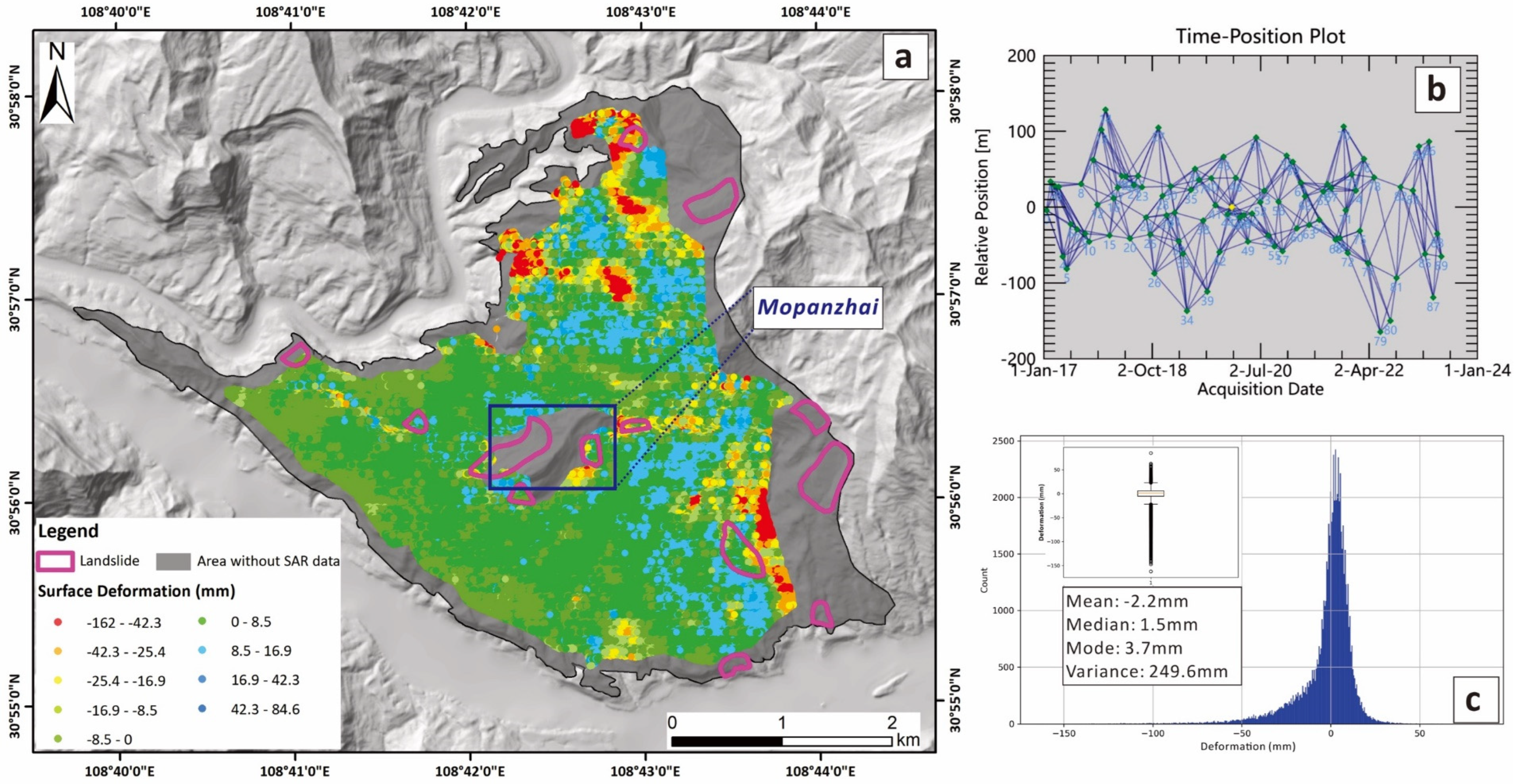
To characterize the observed deformation field and provide the SBAS-InSAR-derived basis for subsequent modeling, we analyzed 89 ascending Sentinel-1 images (European Space Agency, https://search.asf.alaska.edu (accessed on 12 July 2023)) covering the period from 16 January 2017, to 2 June 2023 (Figure 2b). Figure 2 presents the observed surface deformation pattern, data availability, and statistical distribution derived from SBAS-InSAR, rather than the prediction results of the machine learning models. The images were captured at intervals of no less than 24 days. Figure 2a displays the cumulative displacement within the study area over this period. Predominantly, the surface deformation in the region is characterized by downward slope movements, particularly noticeable in the north-western and south-eastern sections. In contrast, the eastern part exhibits significant convex deformations (indicated by blue InSAR dots), suggesting intense human engineering activities, such as artificial filling and house construction, in these areas.
The cumulative displacements are generally normally distributed, with an average value of −2.2 mm. Most of the InSAR interpreted points cluster around 3.7 mm (Figure 2c). However, the variance in cumulative displacements is notably high at 249.6, indicating significant variability in different sections of the study area.
Several challenges arise in accurately assessing surface deformation in our study area due to limitations like the satellite revisit cycle and vegetation cover. These factors lead to numerous missing data points in InSAR observations, predominantly in the central Mopanzhai area and the peripheral areas of the study area. Intriguingly, field surveys reveal significant deformation in these regions, primarily due to landslides. This discrepancy underscores the critical issue of data gaps in traditional InSAR interpretation, posing a significant obstacle to precise deformation analysis.

2.3. Indicator Factors

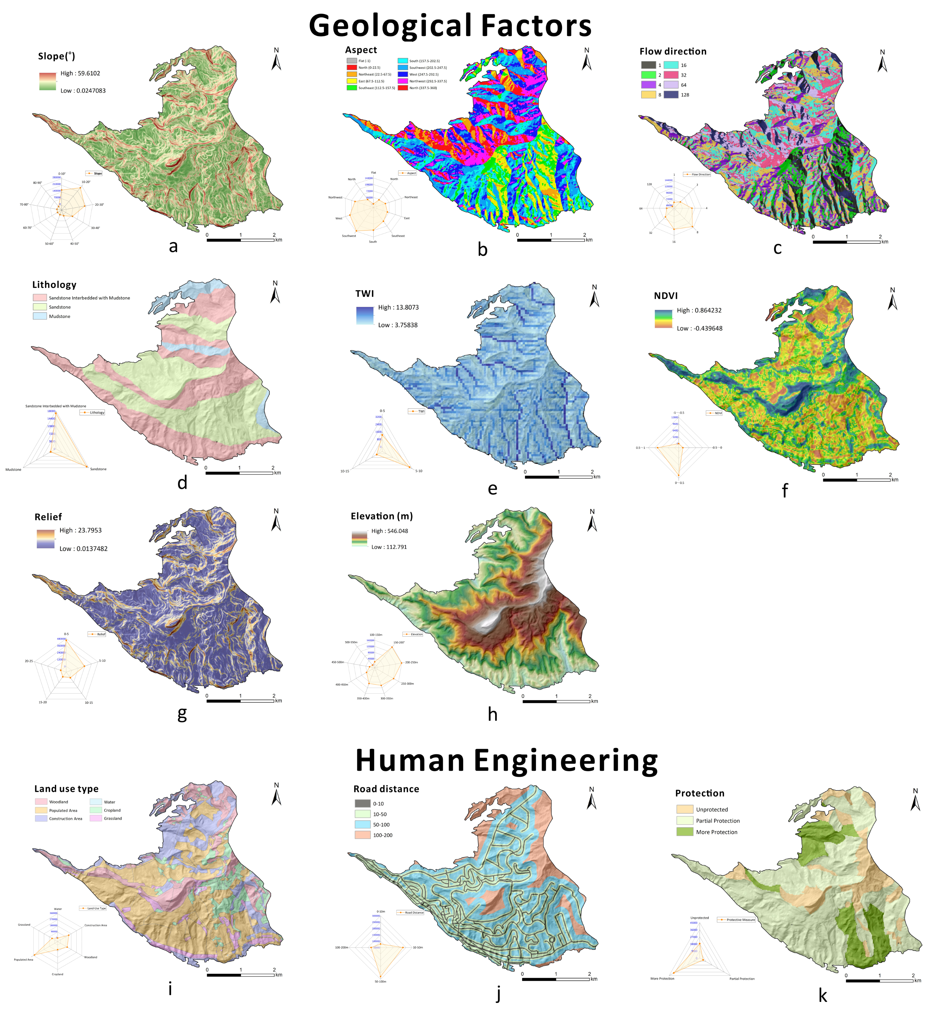
Surface deformation in the study area is jointly controlled by natural conditions and human-engineering disturbance. In addition to topographic and geological controls, rapid urban development has substantially modified local landforms through slope cutting, road construction, land-use change, and protective works, thereby altering deformation patterns and intensities [47,48]. Accordingly, the 11 conditioning factors were selected based on four considerations: their relevance to landslide-related deformation mechanisms, their frequent use in previous deformation and landslide studies, their ability to jointly represent topographic, hydrological, geological, vegetation, and anthropogenic influences, and the availability of spatially continuous data across the study area. The final factor set therefore included topographic variables (elevation, slope, aspect, and relief), hydrological and surface-condition variables (cumulative flow, TWI, and NDVI), geological condition (lithology), and human-engineering factors (land use, distance to roads, and protection level). Among them, land use and lithology were treated as nominal categorical variables, whereas protection level was treated as an ordinal categorical variable. For model input, these variables were encoded as integer class labels according to the thematic maps and field survey records, and their SHAP effects were interpreted after converting the codes back to the original category names rather than by the numerical magnitude of the codes. Comprehensive statistical analysis of these factors further clarifies their respective contributions to surface deformation processes (Figure 3).

3. Methodology

3.1. An Explainable AI (XAI) Framework for Surface Deformation Estimation

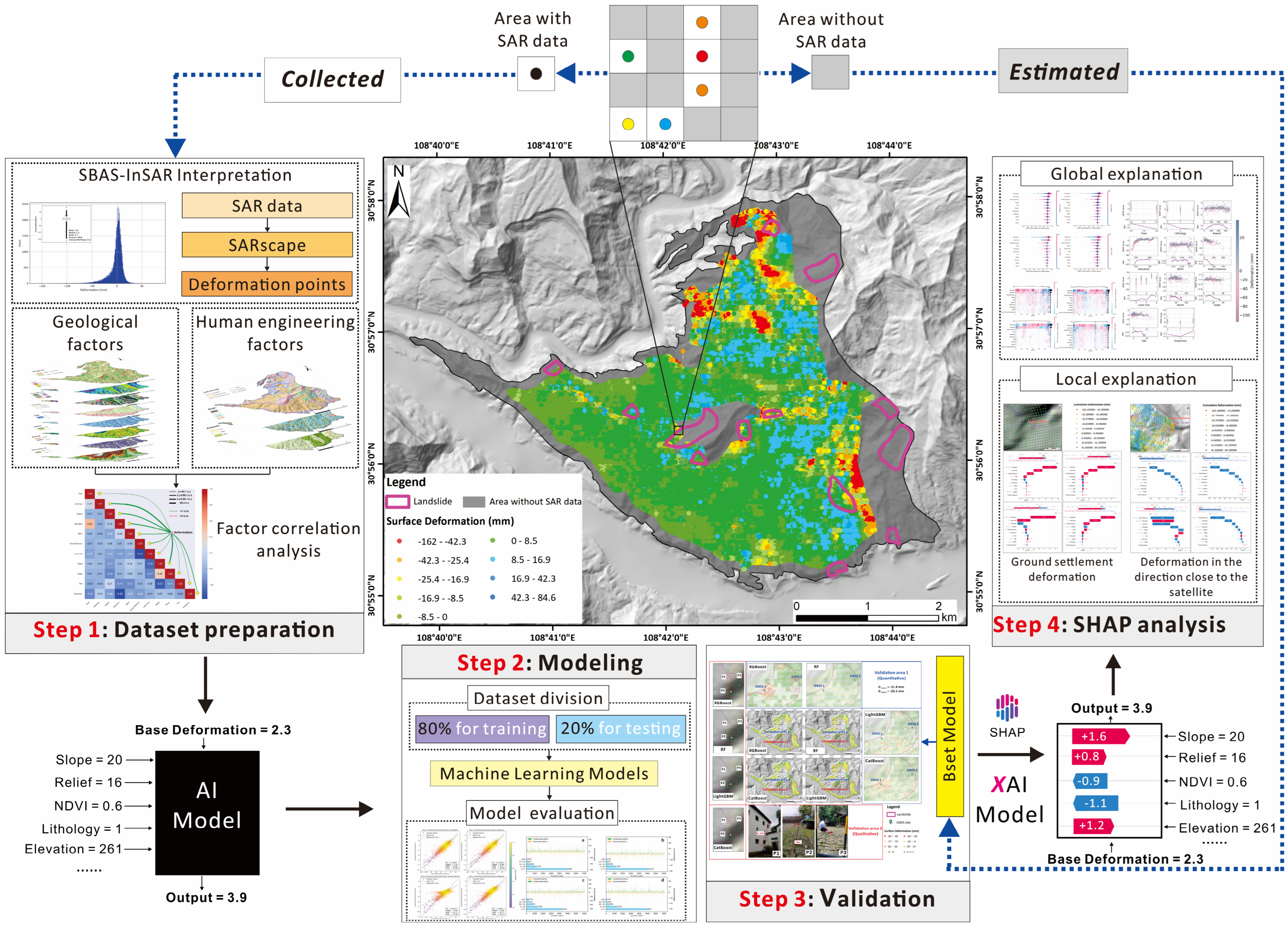
The flowchart of the proposed explainable AI (XAI) framework for surface deformation estimation is presented in Figure 4. First, SAR images of the study area are collected to perform SBAS-InSAR processing, obtaining surface deformation sample points. Subsequently, feature factors are extracted from these samples to construct a dataset. The dataset is then randomly split into 80% for the training set and 20% for the testing set. Four ensemble learning models (LightGBM, XGBoost, Random Forest, and CatBoost) are trained and evaluated using the respective subsets. Based on the performance evaluation, the best-performing model is selected to estimate surface deformation in areas lacking SAR data, and the estimates are validated using field survey data. Finally, the SHAP method is applied to conduct an explanation analysis of the model, aiming to understand whether, how, and to what extent geological and human engineering factors influence the model’s surface deformation estimations.

3.2. XGBoost Model

XGBoost is a representative model in ensemble learning, characterized by its ability to iteratively update and add trees during training to learn the residuals between the predictions of preceding trees and the actual values of the training samples. This approach enables it to effectively capture nonlinear information, making it widely applied in landslide research [49,50]. The core principle of the XGBoost model lies in minimizing the regularized cost function, as illustrated in Equation (1) [51].
L t = i = 1 n l y i , y ^ i t 1 + f t x i + Ω f t
where l denotes the loss function that determines the error between the actual and predicted values, t denotes the number of iterations to minimise the error, Ω f t denotes an additional regularisation term that mitigates model complexity and overfitting, y i corresponds to the actual values and y ^ i represents the predicted values.

3.3. SHAP-Based Machine Learning Model Explanation Method

Recent advancements in machine learning have produced highly accurate but complex models, which often lack interpretability and raise concerns about transparency in critical applications [52]. To overcome these issues, Shapley Additive exPlanations (SHAP) has become a popular and effective approach for explaining machine learning models [53,54]. SHAP, based on cooperative game theory, clearly shows how much each feature contributes to a model’s prediction. This method is particularly useful for understanding how different features interact within the model. The Shapley value for feature i is calculated as follows, based on the formulation of Lundberg and Lee [55]:
ϑ i = S N { i } | S | ! ( n | S | 1 ) ! n ! [ f ( S { i } ) f ( S ) ]
where ϑ i denotes the contribution of feature i , N is the set containing n features, and f ( S { i } ) and f ( S ) represent the model outcomes with and without feature i , respectively.

3.4. SBAS-InSAR

SBAS-InSAR (Small Baseline Subset Synthetic Aperture Radar Interferometry) is a surface deformation monitoring technique based on Synthetic Aperture Radar (SAR) data, widely used in the study of geological disasters, urban subsidence, and large-scale surface deformation [56,57]. The core principle of this method is to analyze phase differences between SAR images acquired at different time points, thereby obtaining ground deformation information [58]. SBAS-InSAR utilizes the Small Baseline Subset approach, selecting SAR images that are geometrically and temporally close to each other for interferometric processing, which helps minimize atmospheric effects, orbital errors, and other sources of interference, thus enhancing monitoring accuracy [59,60]. The formula for interpreting surface deformation using the SBAS-InSAR method is given in Equation (3) [47,61]:
ϕ = 4 π λ d L O S + ϕ a t m + ϕ o r b i t + ϕ n o i s e
where ϕ represents the observed interferometric phase difference, λ denotes the radar wavelength, and d L O S indicates the surface displacement in the line-of-sight (LOS) direction. The terms ϕ a t m , ϕ o r b i t , and ϕ n o i s e correspond to the phase errors caused by atmospheric disturbances, orbital inaccuracies, and other noise effects, respectively.

3.5. Data Collection and Transformation

Multiple spatial datasets were collected to construct the surface deformation prediction model, including SBAS-InSAR-derived deformation observations, topographic and hydrological factors, vegetation information, geological data, land-use information, road data, and field-survey-based protection data. The original datasets included both raster and vector formats. Specifically, the deformation target variable was derived from 89 ascending Sentinel-1 images processed using the SBAS-InSAR approach, whereas elevation, slope, aspect, relief, cumulative flow, TWI, and NDVI were obtained from raster-based terrain or remote-sensing products. Lithology, land use, road networks, and protection measures were derived from thematic maps, interpreted spatial data, or field survey records, with some of these layers originally stored in vector format.
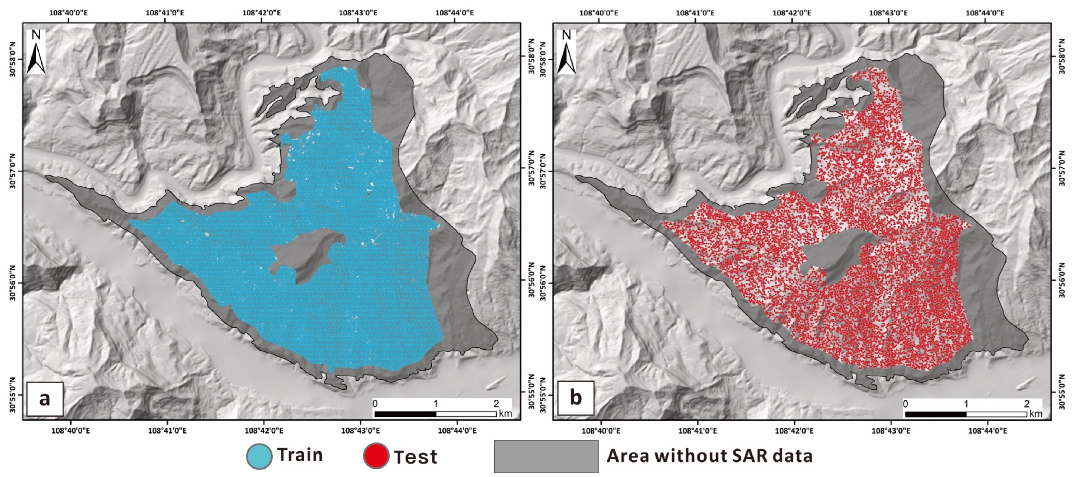
To prepare the datasets for modeling, both the satellite imagery and the ancillary spatial data were transformed into a common analytical framework. First, the 89 ascending Sentinel-1 images were processed using the SBAS-InSAR workflow to derive cumulative line-of-sight surface deformation observations, which served as the target variable of the model. The ancillary spatial datasets were then clipped to the study area, projected to a common coordinate system, and transformed to a unified spatial framework. Raster layers were resampled to a common spatial resolution of 30 m, while vector layers were rasterized or converted into derived raster variables where necessary. For example, the road network was transformed into a distance-to-road raster, and categorical thematic layers such as land use, lithology, and protection level were reclassified according to the classes used in this study. After spatial alignment and transformation, the values of the 11 conditioning factors were extracted at the locations of the SBAS-InSAR deformation samples to build the final modeling dataset. This resulted in 70,780 samples, each containing one deformation value and 11 predictor variables, which were subsequently divided into training (80%) and testing (20%) subsets.

4. Modeling and Results

4.1. Modeling and Validation Process

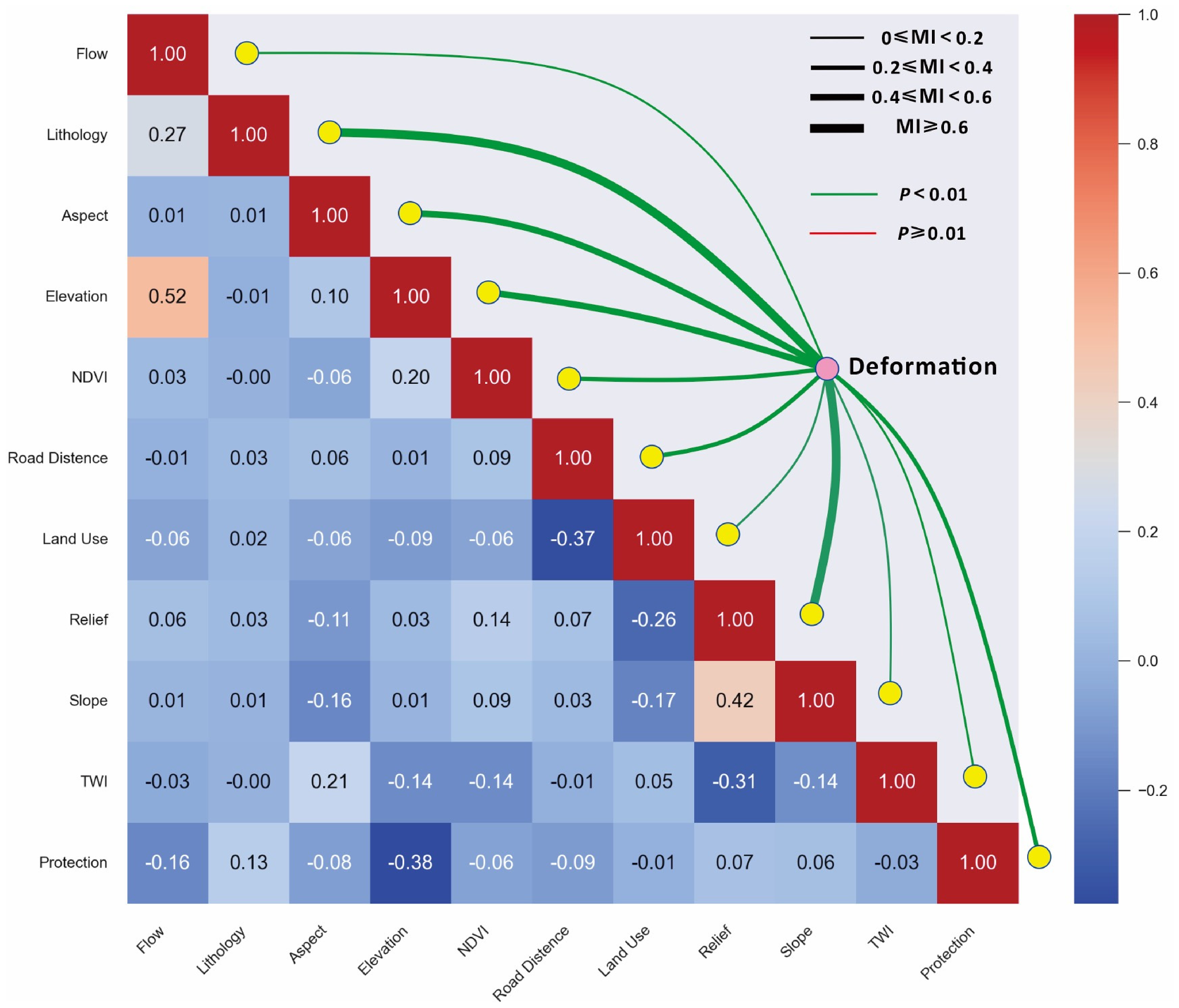
Assessing the independence and predictive value of input factors is essential for robust machine learning modeling. Here, we calculated correlation coefficients between the 11 selected factors and visualized the results as heat maps (Figure 5), which revealed generally low inter-factor correlations, supporting their relative independence. Mutual information (MI, Equation (4)) analysis further showed that lithology and topographic relief had the strongest associations with surface deformation. Finally, all 11 factors were found to be statistically significant predictors of surface deformation (p < 0.01), highlighting their utility for data-driven prediction.
I X i Y = x X , y Y p x , y log p x , y p x p y
In this study, a dataset comprising 70,780 SBAS-InSAR deformation points was established, incorporating both geological and engineering related variables (Figure 6). To assess the predictive capability of ensemble learning for surface deformation, four advanced models, Random Forest (RF), eXtreme Gradient Boosting (XGBoost), LightGBM, and CatBoost, were implemented using the Pycharm platform (v2024.3.6). The dataset was randomly divided, with 80% (56,624 points) allocated for model training and the remaining 20% (14,156 points) reserved for independent testing. Model validation was conducted in two stages. First, internal validation was performed on the testing subset using R2, RMSE, MSE, and MAE to quantitatively evaluate predictive performance. Second, external validation was carried out in SAR data gap areas using independent GNSS measurements in Validation area 1 and field observed damage features in Validation area 2. For the GNSS based validation, the predicted deformation at each benchmark was calculated as the mean value of the ten nearest model grid points and compared with the measured GNSS deformation after conversion to the line of sight direction. This combined validation strategy allowed both numerical accuracy and spatial reliability of the model predictions to be assessed.

4.2. Model Performance Evaluation

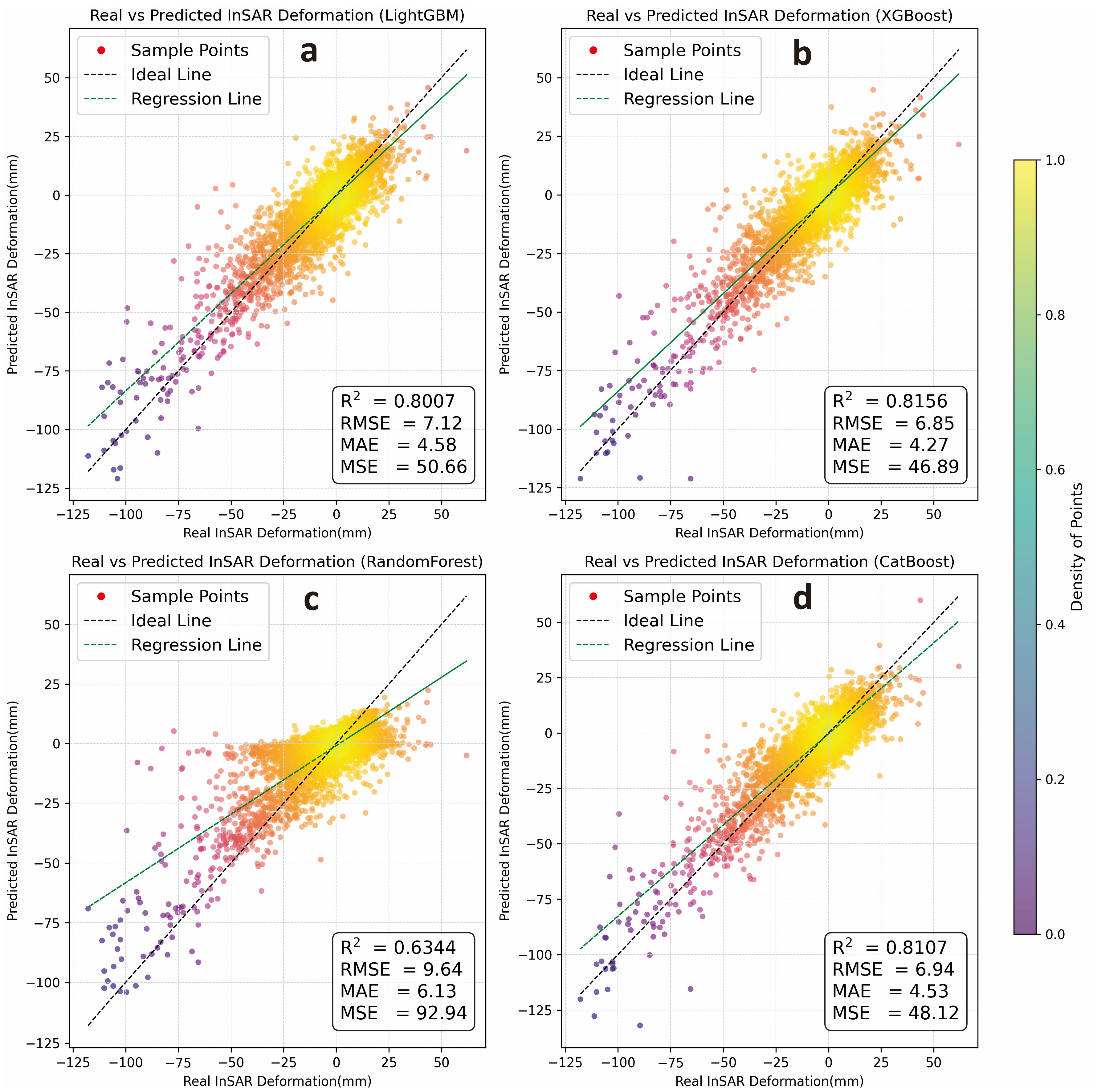
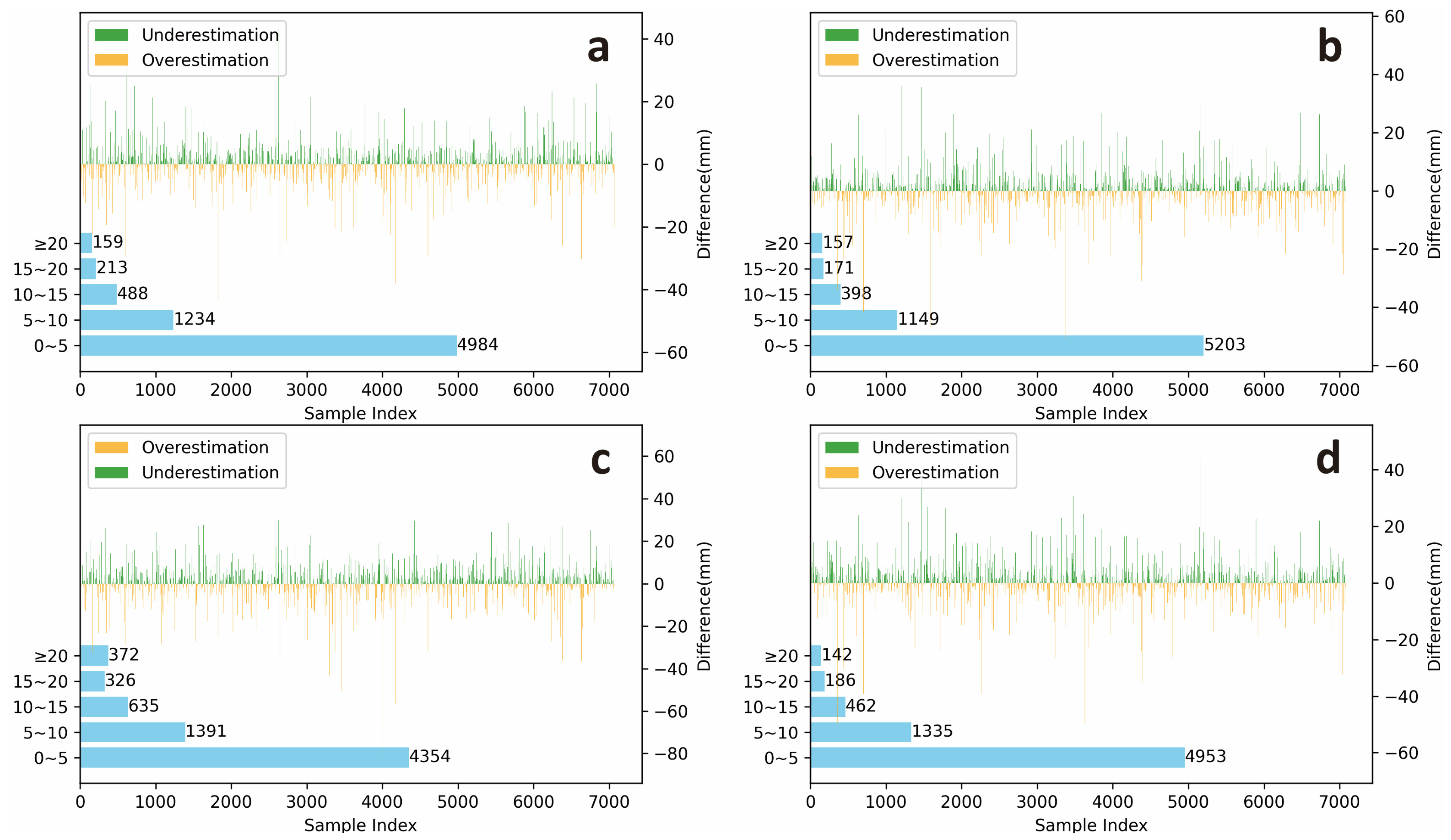
The overall performance of the four models is highly satisfactory, with the XGBoost model standing out. It achieved the highest R2 value (0.8156), and its error metrics (RMSE, MSE, and MAE) were all superior to those of the RF model and the other ensemble learning models (Figure 7). However, all four models exhibited some degree of overestimation or underestimation in their predictions (Figure 8). Most of the absolute errors fell within the range of 0 to 5 mm, followed by the 5 to 10 mm range, with only a few samples showing absolute errors greater than 10 mm, indicating that the overall predictive performance of the models is reliable. Notably, the underestimation errors in the XGBoost model were the smallest among the four models, generally remaining within 5 mm. This superior performance likely reflects the fact that XGBoost iteratively corrects residual errors while incorporating explicit regularization, shrinkage, and column subsampling, which can improve generalization for structured tabular data with complex nonlinear feature interactions [51]. By contrast, Random Forest reduces variance by averaging many independently grown trees [62], but it does not sequentially correct previous errors, which may partly explain its weaker ability to reproduce the spatial deformation gradients observed in this study. LightGBM and CatBoost are also powerful boosting frameworks; however, LightGBM is primarily optimized for computational efficiency on large datasets, whereas CatBoost is especially advantageous when categorical variables are explicitly handled during training [63]. In our case, which involved structured predictors with mostly continuous variables and only a few encoded categorical variables, XGBoost appears to have provided the best balance between model flexibility and generalization.

4.3. Surface Deformation Spatial Estimation Results

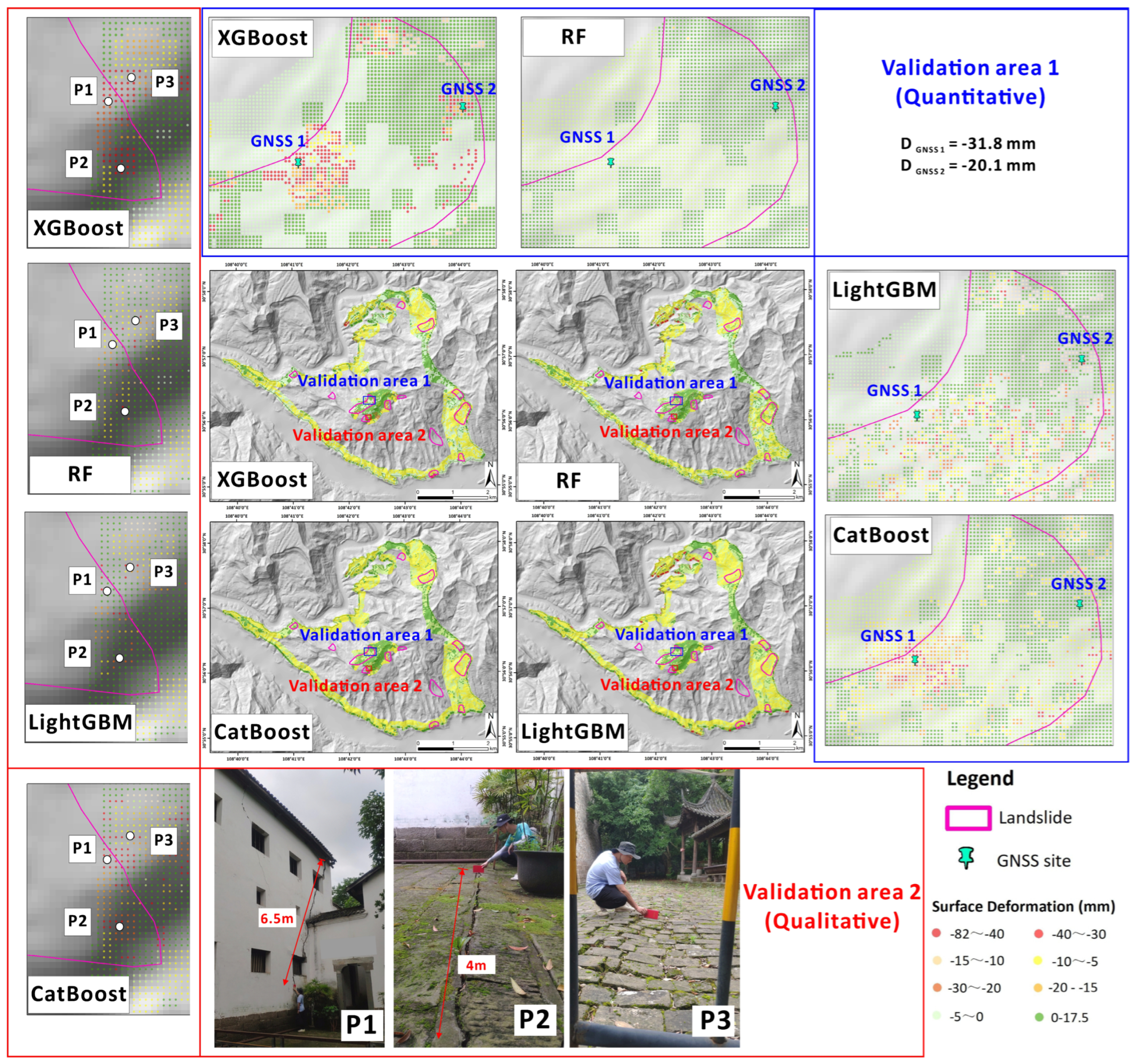
Figure 9 presents a comparison of surface deformation estimates by four machine learning models—XGBoost, Random Forest (RF), LightGBM, and CatBoost—across regions lacking SAR-derived measurements. While all models were trained and tested on the same spatial grid, their outputs reveal clear differences in the spatial coherence and patterns of estimated surface deformation. Both XGBoost and CatBoost yield spatially continuous and geologically plausible deformation zones, closely matching the mapped landslide boundary and geomorphic features. In contrast, the RF model produces highly fragmented and patchy results, failing to reproduce the expected spatial gradients and extent of deformation. LightGBM offers intermediate performance, identifying the overall deformation pattern but occasionally generating discontinuous or irregular estimates.
Quantitative assessment using GNSS benchmarks (Validation area 1, Figure 9), as summarized in Table 1, further supports these visual observations. For both GNSS sites, the XGBoost estimates (−31.2 mm for GNSS 1 and −19.8 mm for GNSS 2) show minimal deviation from the measured values (−31.8 mm and −20.1 mm, respectively), with absolute errors of 0.6 mm and 0.3 mm. CatBoost also demonstrates high accuracy at GNSS 1 (−30.5 mm, error 1.3 mm) but shows a larger error at GNSS 2 (−4.8 mm, error 15.3 mm). By contrast, RF not only underestimates the magnitude of deformation but also predicts the wrong deformation direction at both sites, resulting in large errors (27.5 mm and 22.7 mm). LightGBM underestimates the magnitude at GNSS 1 (−9.9 mm, error 21.9 mm), but performs somewhat better at GNSS 2 (−15.7 mm, error 4.4 mm).
Qualitative validation in Validation area 2 further demonstrates the practical significance of the model results (Figure 9). Field observations, including building wall offsets and pavement displacement, are best matched by the deformation zones identified by XGBoost and CatBoost, both of which delineate contiguous areas of severe subsidence (deformation < −40 mm). LightGBM also captures the main affected area but with lower estimated severity, whereas RF fails to identify any coherent high-deformation zone consistent with the documented structural damage.
Together, the integrated quantitative and qualitative validations indicate that XGBoost and CatBoost provide more reliable and spatially consistent estimates of surface deformation in SAR data-scarce regions, offering strong potential for landslide hazard assessment and mitigation in similar environments.

4.4. Global Explanation Analysis of Models Using SHAP

In this subsection, SHAP and PDP were jointly used to interpret the surface deformation prediction models. SHAP was applied to quantify the direction and magnitude of feature contributions at both the global and sample levels, whereas PDP was used to summarize the average response of model predictions to changes in individual predictors. Together, these methods provide a more coherent interpretation framework by combining contribution-based explanation with trend-based effect visualization. For categorical predictors, SHAP values were interpreted after converting the encoded labels back to the corresponding land-use classes, lithological units, and protection categories.
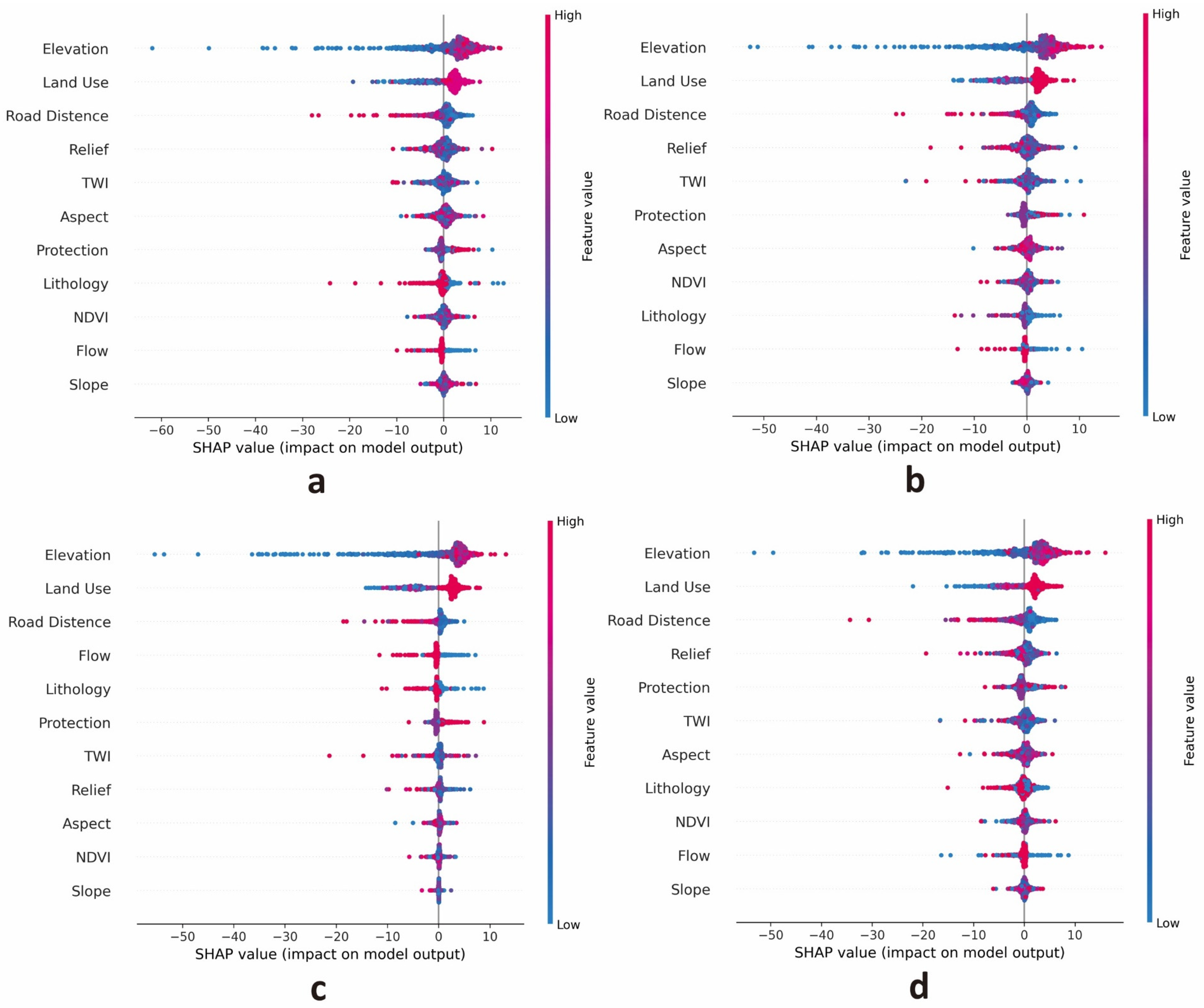
Across all four models (LightGBM, Random Forest, XGBoost and CatBoost), the SHAP summary plots (Figure 10) consistently identify low elevation, intensive land use, proximity to roads and mudstone lithology as the strongest drivers of negative contributions—that is, the greatest predicted subsidence. Samples at higher elevations, under forest cover, located farther than 200 m from roads or sitting on sandstone show SHAP values near zero or slightly positive, indicating stability. Although minor influences appear for relief, aspect, NDVI and wetness index, their SHAP distributions remain tightly clustered around zero in every model.
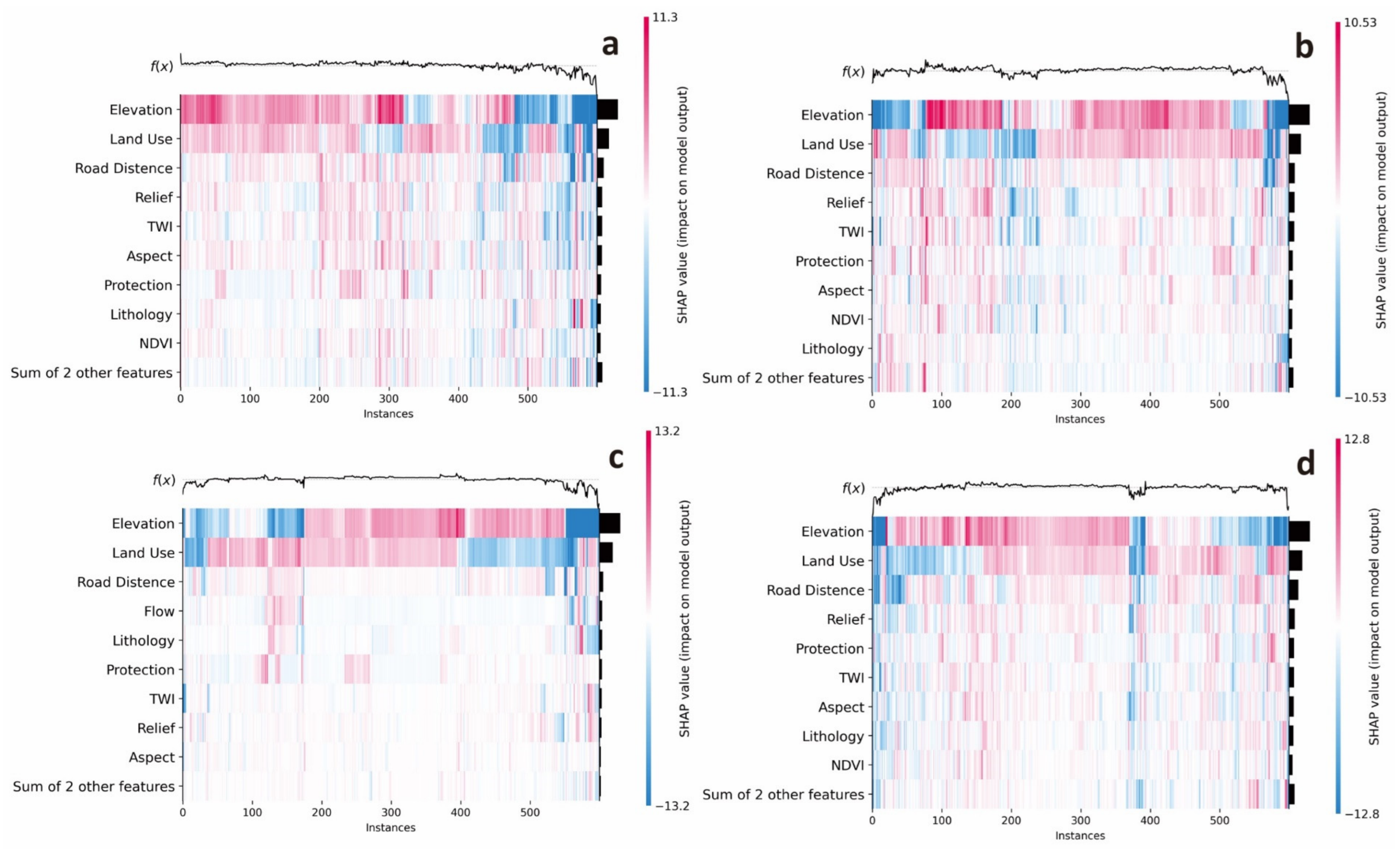
The instance-level SHAP heatmaps (Figure 11) zoom in on the worst-case scenarios: the rows corresponding to elevation, land use, road distance and lithology display intense red bands for exactly the same samples whose cumulative SHAP impact is most negative. In other words, every location predicted to subside most severely combines low ground, cropland or grassland cover, close road proximity and mudstone substrate. By contrast, samples on high ground with construction land or protected forest sitting on sandstone exhibit much cooler colors, confirming their low-risk status.
Model-to-model differences emerge in the range and outlier behavior of SHAP values. LightGBM and Random Forest produce broader SHAP spreads and more extreme negative outliers, reflecting higher sensitivity to these key features, whereas XGBoost and CatBoost yield tighter, more uniform SHAP distributions—suggesting greater robustness and smoother marginal effects. Together, these visualizations not only rank the global importance of natural versus anthropogenic controls but also pinpoint the precise feature combinations that generate the highest subsidence risk in our study area.
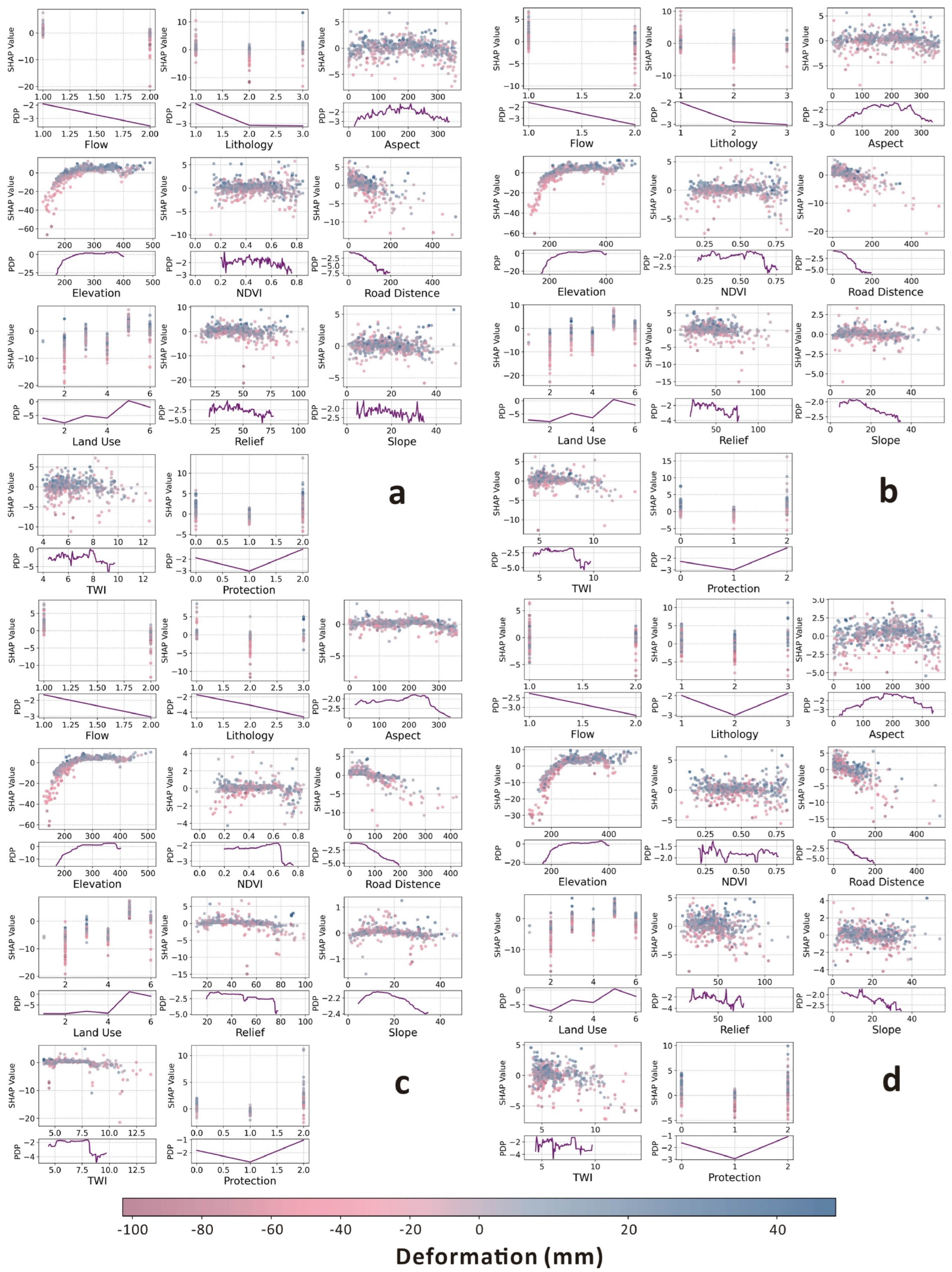
Figure 12 presents the combined SHAP scatterplots (top) and PDP curves (bottom) for LightGBM (Figure 12a), XGBoost (Figure 12b), Random Forest (Figure 12c) and CatBoost (Figure 12d). All models consistently show that human-engineering factors—road distance, land-use class and protection level—dominate predicted subsidence, while cumulative flow, elevation, slope and relief set a secondary baseline and lithology, NDVI and TWI remain near zero. Notably, XGBoost delivers the tightest SHAP distributions and the smoothest PDP curves—reflecting its robust handling of feature interactions and regularization. By contrast, Random Forest exhibits the widest SHAP spreads and more jagged PDP oscillations, indicating higher sensitivity to local heterogeneity and aligning with its comparatively lower accuracy.
Road distance emerges as the single strongest driver of negative SHAP contributions. SHAP points within 0–50 m of a road cluster between −6 and −8 mm, indicating severe settlement risk, then moderate to −2 to −4 mm at 50–150 m and converge near zero beyond 200 m. PDP curves mirror this steep attenuation, reflecting how vibrations, altered drainage and embankment loading dissipate rapidly with distance from linear infrastructure.
Land-use effects appear as clear SHAP “steps”: urban built-up areas center around −5 to −7 mm, cropland −4 to −5 mm, shrubland −2 to −3 mm and forest near zero. PDPs reproduce these marginal jumps, matching field observations that impervious surfaces and deep tillage compact soils and alter groundwater regimes, whereas wooded cover maintains stability.
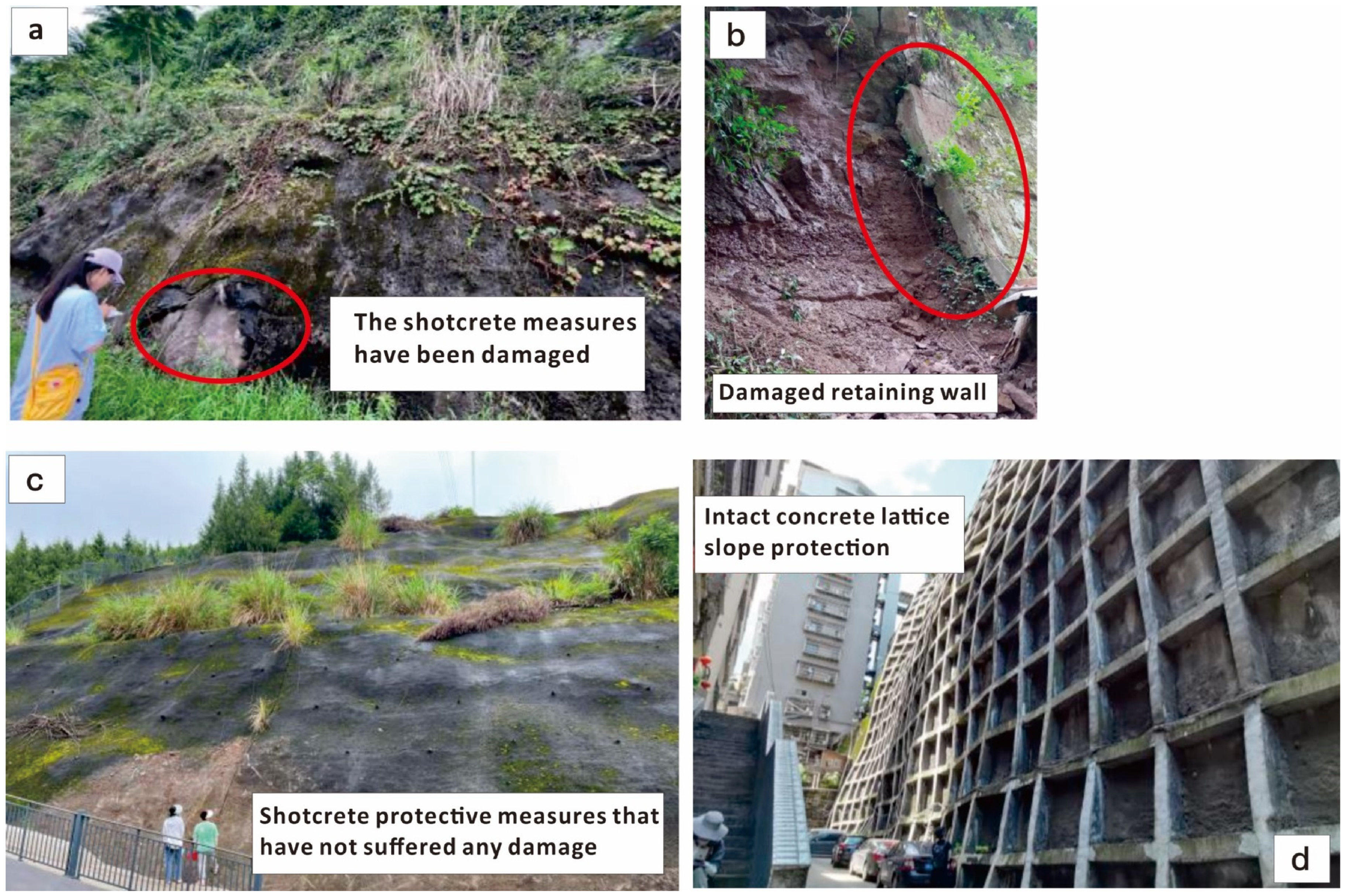
Interestingly, both SHAP and PDP reveal a counter-intuitive V-shaped relationship between protection level and subsidence risk: intermediate, partial protections (level 2) exhibit the deepest PDP trough (−2.5 to −3.5 mm) and most negative SHAP contributions, whereas areas with no protection (level 1) or full protection (level 3) show only moderate settlement (−1 to −2 mm). This pattern contradicts the expectation that “more protection = less deformation,” suggesting instead that mid-tier works may underperform. We therefore hypothesize that partial structures—shallow retaining walls, surface drains and sealants—lose effectiveness when damaged or clogged, leading to peak subsidence in these areas. To verify this, we conducted field surveys across all three protection levels and observed extensive cracking, sediment buildup and seepage damage in level 2 installations, while level 3 systems remained intact and level 1 slopes settled uniformly as expected (Figure 13). These site observations confirm the SHAP-based insights, underscore the necessity of routine inspection and maintenance of intermediate protective works, and demonstrate how interpretability methods can reveal nuanced, non-monotonic effects that traditional importance rankings would overlook.

5. Discussion

5.1. Understanding Human Engineering Impacts on Surface Deformation Through SHAP Local Explanation

Over 80% of the study area is influenced by various types and intensities of anthropogenic activities, which, as demonstrated in the global interpretation in Section 4.4, significantly impact surface deformation. In this subsection, two specific cases are selected to apply the SHAP local interpretation approach, aiming to quantitatively analyze how the characteristics of these anthropogenic activities influence the model’s predictive behavior.
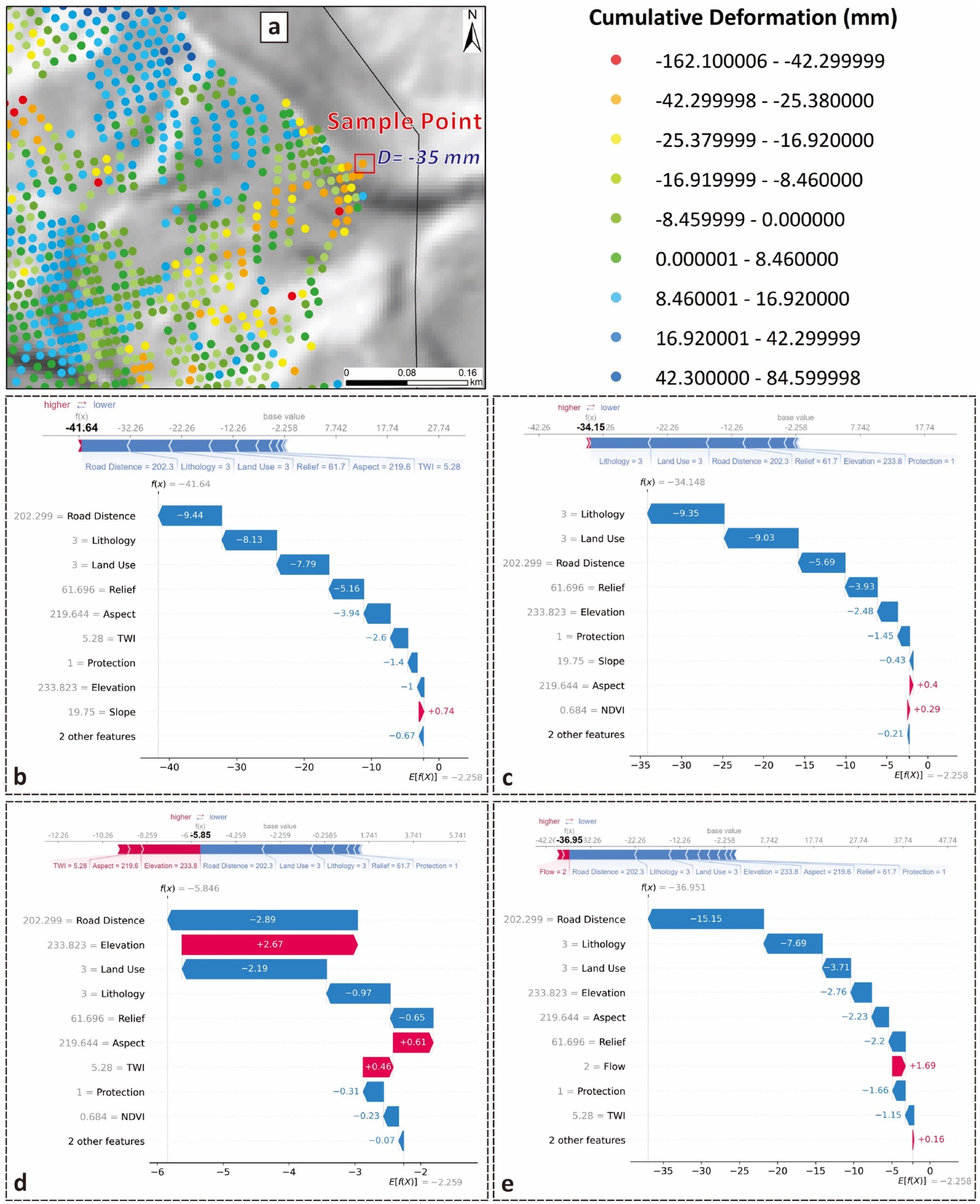
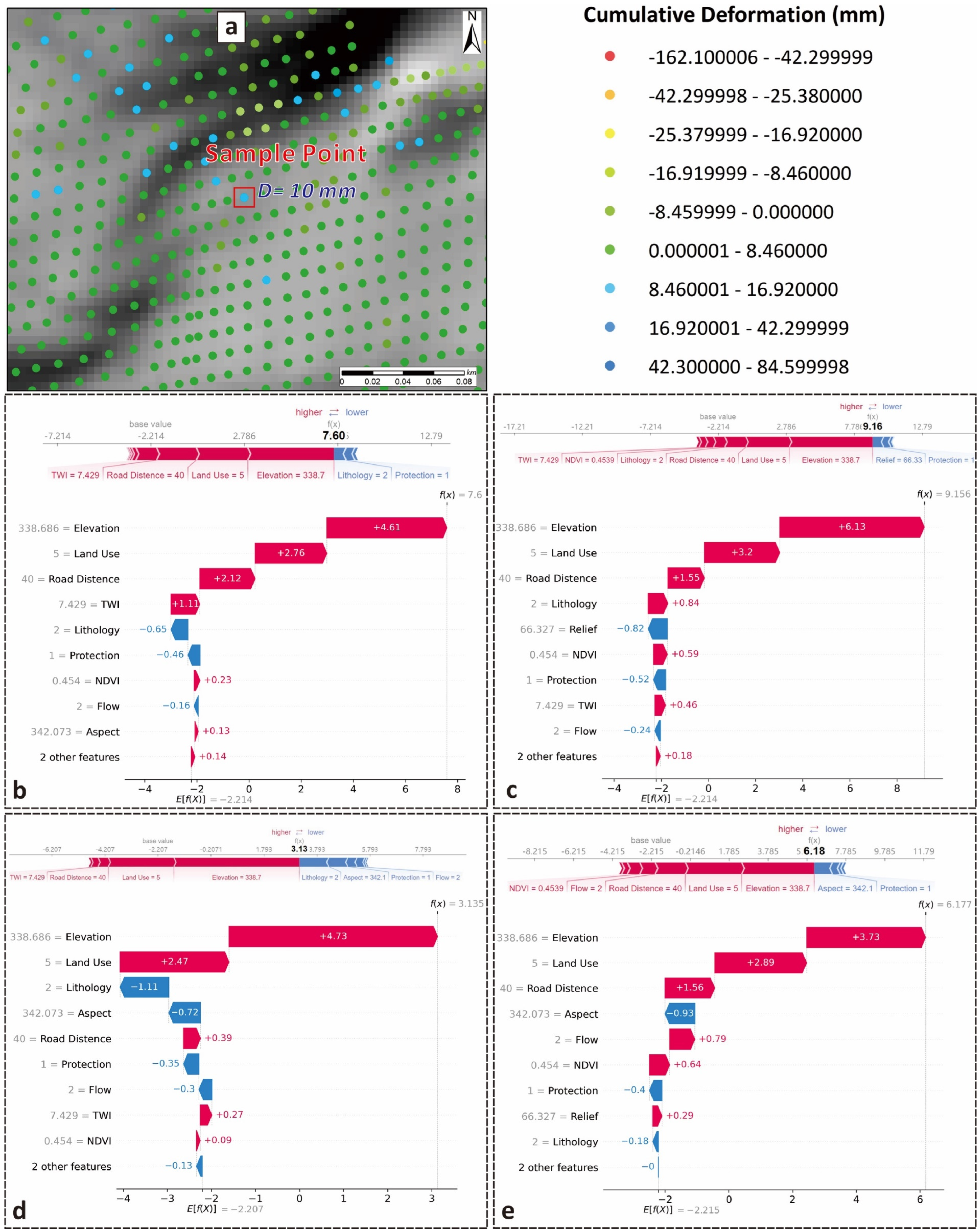
A downward slope deformation sample with a surface deformation of −35 mm was selected for analysis (Figure 14a). The values of each characterization factor for this sample are labeled on the y-axis in Figure 14b–e. Notably, the land use type for this sample is 3, indicating grassland; the lithology is 3, representing mudstone; and the protection measure is 1, denoting partial protection.
Figure 14b–e illustrate the complete prediction process of the four models, highlighting the extent to which each feature influences the predicted values. Overall, all four models correctly predict the direction of surface deformation for the sample. The XGBoost model achieves the most accurate prediction, with a final surface deformation of −34.15 mm and an error of just 0.85 mm. The LightGBM and CatBoost models predict surface deformations of −41.64 mm and −36.95 mm, respectively. While their errors are larger than that of XGBoost, both remain within 7 mm. In contrast, the Random Forest model predicts a surface deformation of −5.85 mm, yielding the largest error among the models at 29.15 mm. Notably, two anthropogenic factors—land use type and distance from roads—play significant roles in the prediction processes of all four models. For instance, in the XGBoost model, which demonstrates the best overall performance, land use type and distance from roads contribute −9.03 mm and −5.69 mm, respectively, to the final predicted value, accounting for nearly half of the total prediction.
Another sample was selected for SHAP local interpretation. In this case, the surface deformation direction aligns with the satellite movement direction, and the degree of deformation is minimal, with a cumulative deformation of only 10 mm (Figure 15a). All four models correctly predicted the deformation direction for this sample. However, regarding specific prediction accuracy, the XGBoost model performed best, predicting a deformation of 9.16 mm with an error of only 0.84 mm. In contrast, the Random Forest model showed the poorest performance, with an error of 6.87 mm.
The significance and specific contributions of the three human-engineering-related features—land use type, distance from roads, and level of protection—varied across the predictions of the four models. Among these, all four models consistently identified land use type (with a value of 5 for this sample, representing construction land) as the most influential human-engineering feature. Furthermore, it ranked as the second most important feature overall, following elevation, in predicting the surface deformation for this sample.
The contributions of land use type to the final predicted deformation values varied across the models: 2.76 mm for LightGBM, 3.2 mm for XGBoost, 2.47 mm for Random Forest, and 2.89 mm for CatBoost, with XGBoost showing the most substantial impact. Construction land typically signifies intense human activities, including building houses and infrastructure, which exert surface loads. Additionally, extensive stabilization measures, such as underground foundations, are often implemented in such areas. This context explains why land use type consistently made a significant positive contribution to the predicted surface deformation across all four models for this sample.
In addition, the anthropogenic feature of distance to the road (with this sample being only 40 m away from the nearest road) was identified as the second most important feature after land use type in the prediction processes of LightGBM, XGBoost, and CatBoost, contributing 2.12 mm, 1.55 mm, and 1.56 mm, respectively. This result suggests that these three models recognize the mitigating effect of roads on surface subsidence. Specifically, the closer the distance to a road, the more likely the predicted direction of surface deformation is to lean towards the positive (i.e., close to the satellite), with a generally smaller deformation magnitude.

5.2. Temporal Limitation and Potential Solution

This paper presents a surface deformation prediction framework using an interpretable ensemble learning model, designed to reliably estimate deformation patterns in areas affected by SAR data gaps. This methodological choice was guided by the nature of the problem. Unlike approaches that focus only on improving InSAR processing itself, the present study addresses the complementary task of estimating deformation in areas where SAR observations are incomplete. In this context, ensemble tree-based models are well suited because they can capture nonlinear relationships and interactions among topographic, hydrological, geological, vegetation, and human engineering factors while remaining effective for structured tabular datasets. Among the tested alternatives, XGBoost was adopted as the preferred model because it provided the best balance between predictive accuracy, spatial coherence, and generalization. SHAP and PDP were further incorporated to complement the predictive model with transparent interpretation, which is essential in landslide studies where understanding the contribution of controlling factors is as important as obtaining accurate estimates. The method’s effectiveness and practical utility have been confirmed through field investigations and quantitative evaluations. However, some limitations exist, especially related to capturing temporal dynamics.
Deformation data derived from SBAS-InSAR techniques typically show spatial and temporal discontinuities [64]. The proposed framework primarily tackles spatial discontinuities due to SAR data gaps, making it suitable for predicting long-term deformation distributions. However, it currently does not capture temporal variations or allow detailed analysis across different time intervals.
In recent studies, machine learning combined with InSAR time-series data has effectively predicted temporal changes in displacement, including episodic accelerations [65,66,67] and responses to hydrometeorological events [68]. These studies provide deeper insights into landslide behavior and enhance real-time hazard monitoring capabilities [69]. Future research should incorporate temporal dynamics and multi-source displacement data into interpretable machine learning frameworks, aiming for high-resolution and continuous deformation prediction.

5.3. Multi-Source Deformation Data Fusion

The deformation prediction framework proposed in this study effectively leverages InSAR-derived measurements to address spatial data gaps commonly found in steep or challenging terrain. To enhance accuracy and robustness further, future research could integrate additional deformation data from sources such as GNSS, inclinometers, ground-based radar, and other geodetic or geotechnical observations [70].
Incorporating multiple data sources may significantly improve predictive capabilities, particularly in areas with sparse or compromised InSAR coverage [71]. For instance, point-based measurements from GNSS or tiltmeters could serve as validation or supplementary inputs, improving spatial resolution and correcting potential biases [72,73]. Combining satellite remote sensing with ground-based data also enables the detection of more complex and varied deformation phenomena [74,75].
However, merging data from different sources introduces methodological challenges. These data often differ in spatial resolution, sampling rates, noise characteristics, and deformation sensitivities [76,77]. Effective integration thus requires careful preprocessing, standardization of coordinate systems, and potentially advanced assimilation methods to ensure consistency and physical realism. Additionally, the limited and uneven distribution of ground-based monitoring stations poses practical challenges to comprehensive integration efforts at larger scales.

5.4. Transferability of the Proposed Framework

Although developed for Yunyang County, the proposed framework is not site-specific in principle and should be transferable to other regions where surface deformation is controlled by comparable combinations of topography, lithology, hydrological setting, vegetation cover, and human-engineering disturbance, and where reliable InSAR observations are available for at least part of the study area to train the model. The framework is expected to perform particularly well in mountainous or hilly urban and peri-urban environments characterized by moderate to strong relief, heterogeneous land use, dense road networks, excavated or engineered slopes, and slow to moderate deformation processes that can be captured by cumulative InSAR measurements. Under such conditions, the selected predictors can represent the dominant controls on deformation, and the SHAP-based interpretation remains physically meaningful.
By contrast, direct application to other regions may require adaptation when the dominant deformation mechanisms differ substantially from those in the present study. In areas controlled primarily by deep-seated landslides, rapid failures, mining subsidence, strong seasonal hydrology, reservoir-level fluctuations, earthquake forcing, or permafrost-related processes, the predictor set should be revised to include locally relevant variables, such as rainfall, groundwater conditions, fault proximity, seismic intensity, or reservoir fluctuation indices. In addition, categorical variables such as lithology, land use, and protection level should be reclassified according to local mapping schemes, the spatial resolution should be adjusted to the scale of local slope processes, and the model should be retrained and validated using locally representative InSAR observations and, where available, ground-based monitoring data. Therefore, the proposed approach is best considered a transferable workflow rather than a fixed model, and its successful application elsewhere depends on the match between local deformation mechanisms, predictor design, and available observations.

6. Conclusions

To address the persistent challenge of accurately estimating surface deformation in areas with incomplete SAR data, this study presents a spatial estimation framework that leverages machine learning and model interpretability techniques. By combining SBAS-InSAR measurements with geological and human engineering factors, the framework captures the complex influences shaping ground deformation and enables spatially complete mapping even in data-scarce settings.
(i)
In Yunyang County, Chongqing, we compiled 11 geological and anthropogenic variables—including protective measures, road proximity and land use—to train four ensemble models. XGBoost yielded the highest predictive skill (R2 = 0.816, RMSE = 6.85 mm, MAE = 4.27 mm, MSE = 46.9). Quantitative comparison with two independent GNSS benchmarks showed that XGBoost reproduced measured subsidence within 0.6 mm at GNSS 1 and 0.3 mm at GNSS 2, outperforming all other models; CatBoost was accurate at GNSS 1 (1.3 mm error) but underestimated deformation at GNSS 2 (15.3 mm error). Field investigations at three damage sites further confirmed that the two top-ranking models correctly identified continuous high-subsidence zones consistent with onsite evidence.
(ii)
Model interpretability was explored using SHAP and partial dependence analyses, which consistently highlighted elevation and engineering-related factors as the dominant controls on deformation. Specifically, areas at lower elevation and greater distance from roads or cultivated land were more susceptible to downslope movement. Moreover, SHAP-based explanations revealed an unexpected peak in predicted subsidence at protection level 2 (partial protection): regions with intermediate protection—where partial protective measures are prone to damage—exhibited the largest negative contributions. This finding, validated by our field surveys showing that partial protective measures often suffer cracking and clogging, underscores the critical importance of routine inspection and maintenance of protective works.
(iii)
For local interpretation, two representative cases with different deformation directions were selected. The results show that, while the ranking of key predictors was generally consistent across models, the specific contribution of each factor varied. LightGBM, XGBoost, and CatBoost reproduced measured deformation with high fidelity, whereas Random Forest tended to underestimate displacement. Among human engineering facntors, distance from roads and land-use type exerted the strongest effects on the predicted deformation patterns.
By integrating InSAR data, ensemble learning, and model explainability, this framework delivers both accurate and interpretable estimates of surface deformation in regions with limited SAR coverage, supporting more effective landslide monitoring and risk management.

Author Contributions

X.F.: Methodology; Software; Data collection and analysis; Field Investigation; Original draft writing and revision. Y.W.: Funding acquisition; Field investigation; Methodology; Draft review and editing; Supervision. J.D.: Draft review and editing; Funding acquisition; Supervision; Methodology. B.C.: Draft review and editing; Funding acquisition; Supervision; Methodology. Z.H.: Data collection. C.Z.: Draft review and editing. All authors have read and agreed to the published version of the manuscript.

Funding

This research was supported by the National Natural Science Foundation of China [Grant Nos. 4217318 to Juan Du, 42377186 to Bo Chai, and 42077277 to Yang Wang].

Data Availability Statement

The SAR data used in this study are openly available through the Alaska Satellite Facility data portal at https://search.asf.alaska.edu (accessed on 12 July 2023). All other data supporting the findings of this study are available from the corresponding author upon reasonable request.

Conflicts of Interest

The authors declare no competing interests.

References

  1. Ma, S.; Qiu, H.; Zhu, Y.; Yang, D.; Tang, B.; Wang, D.; Wang, L.; Cao, M. Topographic changes, surface deformation and movement process before, during and after a rotational landslide. Remote Sens. 2023, 15, 662. [Google Scholar] [CrossRef] [Scilit]
  2. Qiu, H.; Wei, Y.; Liu, W. Controllable Subsidence and Reasonable Planning May Mitigate Geo-Hazards in Large-Scale Land Creation Area. J. Earth Sci. 2025, 36, 806–811. [Google Scholar] [CrossRef] [Scilit]
  3. Ietto, F.; Conforti, M.; Tolomei, C.; Cella, F.; Cianflone, G. Assessment of slow deformations and landslide modelling in the urban area through a multi-methodological approach. J. Earth Sci. 2025, 36, 717–736. [Google Scholar] [CrossRef] [Scilit]
  4. Ding, Y.; Gong, W.; Cheng, Z.; Tian, S.; Zhao, C.; Chen, C. Model tests of the vertical ground deformation measurement of landslide based on multiple UAV images and its application. Bull. Geol. Sci. Technol. 2023, 42, 267–278. [Google Scholar]
  5. Li, Y.; Chen, M.; Huang, H.; Jiang, N.; Lü, P.; Zhou, J. Deformation evolution law and early warning criterion of Xinhua landslide. Bull. Geol. Sci. Technol. 2024, 43, 227–239. [Google Scholar]
  6. Zhang, J.; Wang, Y.; Feng, X.; Li, Y.; Jin, B.; Zhou, C.; Zhang, X.; Deng, Y. Analysis of spatial-temporal variations in landslide susceptibility assessment considering surface deformation and land use dynamics. Bull. Geol. Sci. Technol. 2024, 43, 184–195. [Google Scholar]
  7. Kovács, I.P.; Czigány, S.; Dobre, B.; Fábián, S.Á.; Sobucki, M.; Varga, G.; Bugya, T. A field survey–based method to characterise landslide development: A case study at the high bluff of the Danube, south-central Hungary. Landslides 2019, 16, 1567–1581. [Google Scholar] [CrossRef] [Scilit]
  8. Zhao, W.; Wang, R.; Liu, X.; Ju, N.; Xie, M. Field survey of a catastrophic high-speed long-runout landslide in Jichang Town, Shuicheng County, Guizhou, China, on 13 July 2019. Landslides 2020, 17, 1415–1427. [Google Scholar] [CrossRef] [Scilit]
  9. Xie, M.; Zhao, W.; Ju, N.; He, C.; Huang, H.; Cui, Q. Landslide evolution assessment based on InSAR and real-time monitoring of a large reactivated landslide, Wenchuan, China. Eng. Geol. 2020, 277, 105781. [Google Scholar] [CrossRef] [Scilit]
  10. Darvishi Boloorani, A.; Darvishi, M.; Weng, Q.; Liu, X. Post-war urban damage mapping using InSAR: The case of Mosul City in Iraq. ISPRS Int. J. Geo-Inf. 2021, 10, 140. [Google Scholar] [CrossRef] [Scilit]
  11. Tavakkoliestahbanati, A.; Milillo, P.; Kuai, H.; Giardina, G. Pre-collapse spaceborne deformation monitoring of the Kakhovka dam, Ukraine, from 2017 to 2023. Commun. Earth Environ. 2024, 5, 145. [Google Scholar] [CrossRef] [Scilit]
  12. Yang, K.; Yan, L.; Huang, G.; Chen, C.; Wu, Z. Monitoring building deformation with InSAR: Experiments and validation. Sensors 2016, 16, 2182. [Google Scholar] [CrossRef] [Scilit]
  13. Mohamadi, B.; Balz, T.; Younes, A. Towards a PS-InSAR based prediction model for building collapse: Spatiotemporal patterns of vertical surface motion in collapsed building areas: Case study of Alexandria, Egypt. Remote Sens. 2020, 12, 3307. [Google Scholar] [CrossRef] [Scilit]
  14. Li, Q.; Wang, W.; Wang, J.; Zhang, J.; Geng, D. Exploring the relationship between InSAR coseismic deformation and earthquake-damaged buildings. Remote Sens. Environ. 2021, 262, 112508. [Google Scholar] [CrossRef] [Scilit]
  15. Dong, S.; Samsonov, S.; Yin, H.; Ye, S.; Cao, Y. Time-series analysis of subsidence associated with rapid urbanization in Shanghai, China measured with SBAS InSAR method. Environ. Earth Sci. 2014, 72, 677–691. [Google Scholar] [CrossRef] [Scilit]
  16. Hetland, E.A.; Musé, P.; Simons, M.; Lin, Y.N.; Agram, P.S.; DiCaprio, C.J. Multiscale InSAR time series (MInTS) analysis of surface deformation. J. Geophys. Res. Solid Earth 2012, 117, B02404. [Google Scholar] [CrossRef] [Scilit]
  17. Sun, Q.; Zhang, L.; Ding, X.L.; Hu, J.; Li, Z.W.; Zhu, J.J. Slope deformation prior to Zhouqu, China landslide from InSAR time series analysis. Remote Sens. Environ. 2015, 156, 45–57. [Google Scholar] [CrossRef] [Scilit]
  18. Schlögel, R.; Doubre, C.; Malet, J.P.; Masson, F. Landslide deformation monitoring with ALOS/PALSAR imagery: A D-InSAR geomorphological interpretation method. Geomorphology 2015, 231, 314–330. [Google Scholar] [CrossRef] [Scilit]
  19. Dong, S.; Samsonov, S.; Yin, H.; Huang, L. Two-dimensional ground deformation monitoring in Shanghai based on SBAS and MSBAS InSAR methods. J. Earth Sci. 2018, 29, 960–968. [Google Scholar] [CrossRef] [Scilit]
  20. Rosi, A.; Tofani, V.; Tanteri, L.; Tacconi Stefanelli, C.; Agostini, A.; Catani, F.; Casagli, N. The new landslide inventory of Tuscany (Italy) updated with PS-InSAR: Geomorphological features and landslide distribution. Landslides 2018, 15, 5–19. [Google Scholar] [CrossRef] [Scilit]
  21. Bekaert, D.P.; Handwerger, A.L.; Agram, P.; Kirschbaum, D.B. InSAR-based detection method for mapping and monitoring slow-moving landslides in remote regions with steep and mountainous terrain: An application to Nepal. Remote Sens. Environ. 2020, 249, 111983. [Google Scholar] [CrossRef] [Scilit]
  22. Intrieri, E.; Raspini, F.; Fumagalli, A.; Lu, P.; Del Conte, S.; Farina, P.; Allievi, J.; Ferretti, A.; Casagli, N. The Maoxian landslide as seen from space: Detecting precursors of failure with Sentinel-1 data. Landslides 2018, 15, 123–133. [Google Scholar] [CrossRef] [Scilit]
  23. Jiang, Y.; Xu, Q.; Lu, Z. Landslide displacement monitoring by time series InSAR combining PS and DS targets. In IGARSS 2020 IEEE International Geoscience and Remote Sensing Symposium; IEEE: Piscataway, NJ, USA, 2020; pp. 1011–1014. [Google Scholar]
  24. Younsi, S.; Dabiri, H.; Marini, R.; Mazzanti, P.; Scarascia Mugnozza, G.; Bozzano, F. Reconstructing missing InSAR data by the application of machine leaning-based prediction models: A case study of Rieti. J. Civ. Struct. Health Monit. 2024, 14, 143–161. [Google Scholar] [CrossRef] [Scilit]
  25. Wang, Z.; Bai, X. Long-term Time Series Prediction of Deformation in The Area of Pylons By Combining InSAR and Transformer-based. In 2022 Euro-Asia Conference on Frontiers of Computer Science and Information Technology (FCSIT); IEEE: Piscataway, NJ, USA, 2022; pp. 60–63. [Google Scholar]
  26. Ahmed, R.; Siqueira, P.; Hensley, S.; Chapman, B.; Bergen, K. A survey of temporal decorrelation from spaceborne L-Band repeat-pass InSAR. Remote Sens. Environ. 2011, 115, 2887–2896. [Google Scholar] [CrossRef] [Scilit]
  27. Hao, B.; Ma, C.; Zhang, G.; Kang, L. Analyzing decorrelation of multi-temporal SAR data on InSAR. In 2008 Congress on Image and Signal Processing; IEEE: Piscataway, NJ, USA, 2008; Volume 1, pp. 452–461. [Google Scholar]
  28. Chen, Y.; Sun, Q.; Hu, J. Quantitatively estimating of InSAR decorrelation based on landsat-derived NDVI. Remote Sens. 2021, 13, 2440. [Google Scholar] [CrossRef] [Scilit]
  29. Wang, T.; DeGrandpre, K.; Lu, Z.; Freymueller, J.T. Complex surface deformation of Akutan volcano, Alaska revealed from InSAR time series. Int. J. Appl. Earth Obs. Geoinf. 2018, 64, 171–180. [Google Scholar] [CrossRef] [Scilit]
  30. Shen, P.; Wang, C.; Luo, X.; Hu, J.; Wan, J. Interferometric phase reconstruction with temporal decorrelation model constraints for time-series InSAR surface deformation monitoring. Int. J. Digit. Earth 2024, 17, 2426511. [Google Scholar] [CrossRef] [Scilit]
  31. Li, Z.; Cao, Y.; Wei, J.; Duan, M.; Wu, L.; Hou, J.; Zhu, J. Time-series InSAR ground deformation monitoring: Atmospheric delay modeling and estimating. Earth-Sci. Rev. 2019, 192, 258–284. [Google Scholar]
  32. Zwieback, S.; Liu, L.; Rouyet, L.; Short, N.; Strozzi, T. Advances in InSAR analysis of permafrost terrain. Permafr. Periglac. Process. 2024, 35, 544–556. [Google Scholar] [CrossRef] [Scilit]
  33. Xu, G.; Gao, Y.; Li, J.; Xing, M. InSAR phase denoising: A review of current technologies and future directions. IEEE Geosci. Remote Sens. Mag. 2020, 8, 64–82. [Google Scholar] [CrossRef] [Scilit]
  34. Schaefer, L.N.; Di Traglia, F.; Chaussard, E.; Lu, Z.; Nolesini, T.; Casagli, N. Monitoring volcano slope instability with Synthetic Aperture Radar: A review and new data from Pacaya (Guatemala) and Stromboli (Italy) volcanoes. Earth-Sci. Rev. 2019, 192, 236–257. [Google Scholar] [CrossRef] [Scilit]
  35. Yao, S.; He, Y.; Zhang, L.; Yang, W.; Chen, Y.; Sun, Q.; Zhao, Z.; Cao, S. A convLSTM neural network model for spatiotemporal prediction of mining area surface deformation based on SBAS-InSAR monitoring data. IEEE Trans. Geosci. Remote Sens. 2023, 61, 5201722. [Google Scholar] [CrossRef] [Scilit]
  36. Radman, A.; Akhoondzadeh, M.; Hosseiny, B. Integrating InSAR and deep-learning for modeling and predicting subsidence over the adjacent area of Lake Urmia, Iran. GISci. Remote Sens. 2021, 58, 1413–1433. [Google Scholar] [CrossRef] [Scilit]
  37. Brengman, C.M.; Barnhart, W.D. Identification of surface deformation in InSAR using machine learning. Geochem. Geophys. Geosyst. 2021, 22, e2020GC009204. [Google Scholar] [CrossRef] [Scilit]
  38. Huang, Z.; Yu, F. InSAR-derived surface deformation of Chaoshan Plain, China: Exploring the role of human activities in the evolution of coastal landscapes. Geomorphology 2023, 426, 108606. [Google Scholar] [CrossRef] [Scilit]
  39. Fiorentini, N.; Maboudi, M.; Leandri, P.; Losa, M.; Gerke, M. Surface motion prediction and mapping for road infrastructures management by PS-InSAR measurements and machine learning algorithms. Remote Sens. 2020, 12, 3976. [Google Scholar] [CrossRef] [Scilit]
  40. Zheng, L.; Wang, Q.; Cao, C.; Shan, B.; Jin, T.; Zhu, K.; Li, Z. Development and Comparison of InSAR-Based Land Subsidence Prediction Models. Remote Sens. 2024, 16, 3345. [Google Scholar] [CrossRef] [Scilit]
  41. Chang, K.; Zhao, Z.; Zhou, D.; Tian, Z.; Wang, C. Prediction of Surface Subsidence in Mining Areas Based on Ascending-Descending Orbits Small Baseline Subset InSAR and Neural Network Optimization Models. Sensors 2024, 24, 4770. [Google Scholar] [CrossRef] [Scilit]
  42. Al-Najjar, H.A.; Pradhan, B.; Beydoun, G.; Sarkar, R.; Park, H.J.; Alamri, A. A novel method using explainable artificial intelligence (XAI)-based Shapley Additive Explanations for spatial landslide prediction using Time-Series SAR dataset. Gondwana Res. 2023, 123, 107–124. [Google Scholar] [CrossRef] [Scilit]
  43. Zhou, C.; Cao, Y.; Gan, L.; Wang, Y.; Motagh, M.; Roessner, S.; Hu, X.; Yin, K. A novel framework for landslide displacement prediction using MT-InSAR and machine learning techniques. Eng. Geol. 2024, 334, 107497. [Google Scholar] [CrossRef] [Scilit]
  44. He, K.; Tanyas, H.; Chang, L.; Hu, X.; Luo, G.; Lombardo, L. Modelling InSAR-derived hillslope velocities with multivariate statistics: A first attempt to generate interpretable predictions. Remote Sens. Environ. 2023, 289, 113518. [Google Scholar] [CrossRef] [Scilit]
  45. Li, F.; Liu, G.; Tao, Q.; Zhai, M. Land subsidence prediction model based on its influencing factors and machine learning methods. Nat. Hazards 2023, 116, 3015–3041. [Google Scholar] [CrossRef] [Scilit]
  46. Naghibi, S.A.; Khodaei, B.; Hashemi, H. An integrated InSAR-machine learning approach for ground deformation rate modeling in arid areas. J. Hydrol. 2022, 608, 127627. [Google Scholar] [CrossRef] [Scilit]
  47. Dong, S.; Yin, H.; Yao, S.; Zhang, F. Detecting surface subsidence in coal mining area based on DInSAR technique. J. Earth Sci. 2013, 24, 449–456. [Google Scholar] [CrossRef] [Scilit]
  48. Mao, Z.; Jiao, Y.; Tan, F.; Qi, X.; Zeng, C. Susceptibility Mapping of Ground Collapse Caused by Anthropogenic Activities. J. Earth Sci. 2025, 36, 1168–1180. [Google Scholar] [CrossRef] [Scilit]
  49. Kavzoglu, T.; Teke, A. Advanced hyperparameter optimization for improved spatial prediction of shallow landslides using extreme gradient boosting (XGBoost). Bull. Eng. Geol. Environ. 2022, 81, 201. [Google Scholar] [CrossRef] [Scilit]
  50. Shi, N.; Li, Y.; Wen, L.; Zhang, Y. Rapid prediction of landslide dam stability considering the missing data using XGBoost algorithm. Landslides 2022, 19, 2951–2963. [Google Scholar] [CrossRef] [Scilit]
  51. Chen, T.; Guestrin, C. Xgboost: A scalable tree boosting system. In Proceedings of the 22nd ACM SIGKDD International Conference on Knowledge Discovery and Data Mining; ACM: New York, NY, USA, 2016; pp. 785–794. [Google Scholar]
  52. Pradhan, B.; Dikshit, A.; Lee, S.; Kim, H. An explainable AI (XAI) model for landslide susceptibility modeling. Appl. Soft Comput. 2023, 142, 110324. [Google Scholar] [CrossRef] [Scilit]
  53. Li, Z. Extracting spatial effects from machine learning model using local interpretation method: An example of SHAP and XGBoost. Comput. Environ. Urban Syst. 2022, 96, 101845. [Google Scholar] [CrossRef] [Scilit]
  54. Zhang, J.; Ma, X.; Zhang, J.; Sun, D.; Zhou, X.; Mi, C.; Wen, H. Insights into geospatial heterogeneity of landslide susceptibility based on the SHAP-XGBoost model. J. Environ. Manag. 2023, 332, 117357. [Google Scholar] [CrossRef] [Scilit]
  55. Lundberg, S.M.; Lee, S.-I. A unified approach to interpreting model predictions. In Advances in Neural Information Processing Systems; Curran Associates Inc.: Red Hook, NY, USA, 2017; Volume 30. [Google Scholar]
  56. van Natijne, A.L.; Bogaard, T.A.; van Leijen, F.J.; Hanssen, R.F.; Lindenbergh, R.C. World-wide InSAR sensitivity index for landslide deformation tracking. Int. J. Appl. Earth Obs. Geoinf. 2022, 111, 102829. [Google Scholar] [CrossRef] [Scilit]
  57. Manconi, A.; Jones, N.; Loew, S.; Strozzi, T.; Caduff, R.; Wegmueller, U. Monitoring surface deformation with spaceborne radar interferometry in landslide complexes: Insights from the Brienz/Brinzauls slope instability, Swiss Alps. Landslides 2024, 21, 2519–2533. [Google Scholar] [CrossRef] [Scilit]
  58. Lauknes, T.R.; Zebker, H.A.; Larsen, Y. InSAR deformation time series using an L1-norm small-baseline approach. IEEE Trans. Geosci. Remote Sens. 2010, 49, 536–546. [Google Scholar] [CrossRef] [Scilit]
  59. Necsoiu, M.; McGinnis, R.N.; Hooper, D.M. New insights on the Salmon Falls Creek Canyon landslide complex based on geomorphological analysis and multitemporal satellite InSAR techniques. Landslides 2014, 11, 1141–1153. [Google Scholar] [CrossRef] [Scilit]
  60. Chen, Y.; Dong, X.; Qi, Y.; Huang, P.; Sun, W.; Xu, W.; Tan, W.; Li, X.; Liu, X. Integration of DInSAR-PS-stacking and SBAS-PS-InSAR methods to monitor mining-related surface subsidence. Remote Sens. 2023, 15, 2691. [Google Scholar] [CrossRef] [Scilit]
  61. Tizzani, P.; Berardino, P.; Casu, F.; Euillades, P.; Manzo, M.; Ricciardi, G.P.; Zeni, G.; Lanari, R. Surface deformation of Long Valley caldera and Mono Basin, California, investigated with the SBAS-InSAR approach. Remote Sens. Environ. 2007, 108, 277–289. [Google Scholar] [CrossRef] [Scilit]
  62. Breiman, L. Random forests. Mach. Learn. 2001, 45, 5–32. [Google Scholar] [CrossRef] [Scilit]
  63. Prokhorenkova, L.; Gusev, G.; Vorobev, A.; Dorogush, A.V.; Gulin, A. CatBoost: Unbiased boosting with categorical features. In Advances in Neural Information Processing Systems; Curran Associates Inc.: Red Hook, NY, USA, 2018; Volume 31, pp. 6638–6648. [Google Scholar]
  64. Hill, P.; Biggs, J.; Ponce-López, V.; Bull, D. Time-series prediction approaches to forecasting deformation in Sentinel-1 INSAR data. J. Geophys. Res. Solid Earth 2021, 126, e2020JB020176. [Google Scholar] [CrossRef] [Scilit]
  65. Novellino, A.; Cesarano, M.; Cappelletti, P.; Di Martire, D.; Di Napoli, M.; Ramondini, M.; Sowter, A.; Calcaterra, D. Slow-moving landslide risk assessment combining Machine Learning and InSAR techniques. Catena 2021, 203, 105317. [Google Scholar] [CrossRef] [Scilit]
  66. Liu, Z.; Qiu, H.; Zhu, Y.; Liu, Y.; Yang, D.; Ma, S.; Zhang, J.; Wang, Y.; Wang, L.; Tang, B. Efficient identification and monitoring of landslides by time-series InSAR combining single-and multi-look phases. Remote Sens. 2022, 14, 1026. [Google Scholar] [CrossRef] [Scilit]
  67. Zhang, Y.; Meng, X.M.; Dijkstra, T.A.; Jordan, C.J.; Chen, G.; Zeng, R.Q.; Novellino, A. Forecasting the magnitude of potential landslides based on InSAR techniques. Remote Sens. Environ. 2020, 241, 111738. [Google Scholar] [CrossRef] [Scilit]
  68. Xiong, Z.; Zhang, M.; Ma, J.; Xing, G.; Feng, G.; An, Q. InSAR-based landslide detection method with the assistance of C-index. Landslides 2023, 20, 2709–2723. [Google Scholar] [CrossRef] [Scilit]
  69. Zeng, P.; Feng, B.; Dai, K.; Li, T.; Fan, X.; Sun, X. Can satellite InSAR innovate the way of large landslide early warning? Eng. Geol. 2024, 342, 107771. [Google Scholar] [CrossRef] [Scilit]
  70. Yin, Y.; Zheng, W.; Liu, Y.; Zhang, J.; Li, X. Integration of GPS with InSAR to monitoring of the Jiaju landslide in Sichuan, China. Landslides 2010, 7, 359–365. [Google Scholar] [CrossRef] [Scilit]
  71. Carlà, T.; Tofani, V.; Lombardi, L.; Raspini, F.; Bianchini, S.; Bertolo, D.; Thuegaz, P.; Casagli, N. Combination of GNSS, satellite InSAR, and GBInSAR remote sensing monitoring to improve the understanding of a large landslide in high alpine environment. Geomorphology 2019, 335, 62–75. [Google Scholar] [CrossRef] [Scilit]
  72. Yalvac, S. Validating InSAR-SBAS results by means of different GNSS analysis techniques in medium-and high-grade deformation areas. Environ. Monit. Assess. 2020, 192, 120. [Google Scholar] [CrossRef] [Scilit] [PubMed]
  73. Yan, H.; Dai, W.; Xu, W.; Shi, Q.; Sun, K.; Lu, Z.; Wang, R. A method for correcting InSAR interferogram errors using GNSS data and the K-means algorithm. Earth Planets Space 2024, 76, 51. [Google Scholar] [CrossRef] [Scilit]
  74. Fabris, M.; Battaglia, M.; Chen, X.; Menin, A.; Monego, M.; Floris, M. An integrated InSAR and GNSS approach to monitor land subsidence in the Po River Delta (Italy). Remote Sens. 2022, 14, 5578. [Google Scholar] [CrossRef] [Scilit]
  75. Hamling, I.J.; Wright, T.J.; Hreinsdóttir, S.; Wallace, L.M. A snapshot of New Zealand’s dynamic deformation field from Envisat InSAR and GNSS observations between 2003 and 2011. Geophys. Res. Lett. 2022, 49, e2021GL096465. [Google Scholar] [CrossRef] [Scilit]
  76. Parizzi, A.; Rodriguez Gonzalez, F.; Brcic, R. A covariance-based approach to merging InSAR and GNSS displacement rate measurements. Remote Sens. 2020, 12, 300. [Google Scholar] [CrossRef] [Scilit]
  77. Bekaert, D.P.S.; Segall, P.; Wright, T.J.; Hooper, A.J. A network inversion filter combining GNSS and InSAR for tectonic slip modeling. J. Geophys. Res. Solid Earth 2016, 121, 2069–2086. [Google Scholar] [CrossRef] [Scilit]
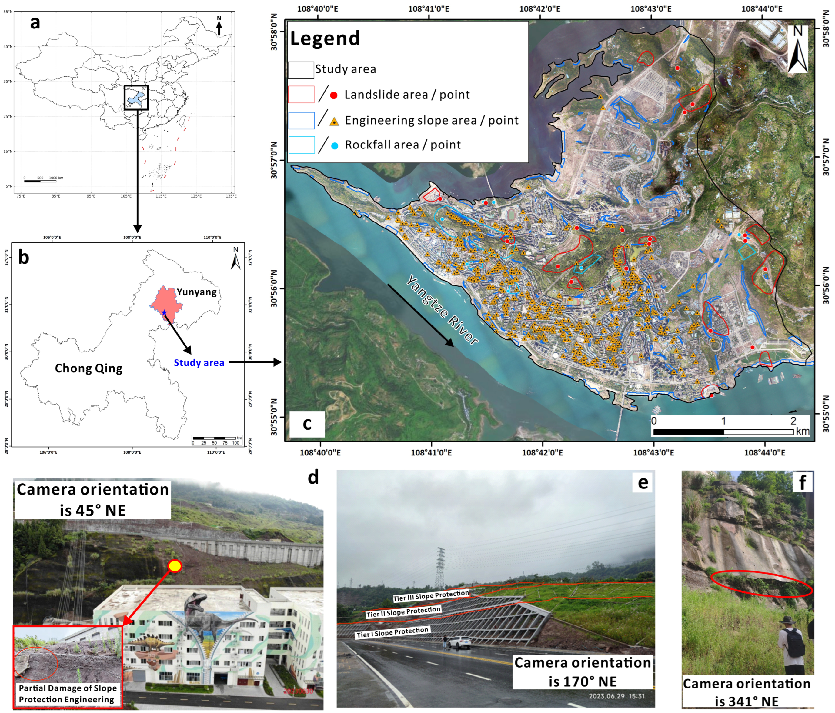
Figure 1. Geographical Location of the Study Area and Distribution of Landslides, Rockfall, and Excavated Slopes Within the Area ((a) location of Chongqing City in China; (b) location of Yunyang County in Chongqing City as well as the location of the study area; (c) remote sensing image of the study area; (df) are three comparatively typical examples of localized damage in protective engineering; engineering slope refers to a slope that has been artificially excavated. Without protective measures, its stability is relatively poor).
Remotesensing 18 01363 g001
Figure 2. SBAS-InSAR-derived observed surface deformation characteristics in the study area ((a) observed surface deformation map with landslide boundaries and SAR data gaps; (b) temporal-spatial baseline plot of SAR acquisitions; (c) statistical distribution of observed surface deformation values).
Remotesensing 18 01363 g002
Figure 3. Distribution statistics of various indicator factors represented by the number of grids (a) slope; (b) aspect; (c) flow direction; (d) lithology; (e) topographic wetness index (TWI); (f) normalized difference vegetation index (NDVI); (g) relief; (h) elevation; (i) land-use type; (j) road distance; (k) protection.
Remotesensing 18 01363 g003
Figure 4. Flowchart of this study.
Remotesensing 18 01363 g004
Figure 5. Correlation heatmap among various indicators (The thickness of the lines is determined by the mutual information score, indicating the degree of correlation with downward slope deformation. Thicker lines represent higher correlation. The color of the lines is determined by p-value testing, signifying the significance of each indicator in estimating downward slope deformation).
Remotesensing 18 01363 g005
Figure 6. Spatial distribution of training and testing dataset ((a) locations of training samples; (b) locations of testing samples; gray areas indicate areas with missing SAR data).
Remotesensing 18 01363 g006
Figure 7. Model performance evaluation ((a) LightGBM; (b) XGBoost; (c) Random Forest; (d) CatBoost).
Remotesensing 18 01363 g007
Figure 8. Statistics of overestimation and underestimation of surface deformation by each model ((a) LightGBM; (b) XGBoost; (c) Random Forest; (d) CatBoost).
Remotesensing 18 01363 g008
Figure 9. Prediction of surface deformation over SAR data gaps via XGBoost, Random Forest, LightGBM and CatBoost, corroborated GNSS measurements and field observations. P1, building wall cracking; P2, pavement displacement/cracking; P3, ground/pavement deformation.
Remotesensing 18 01363 g009
Figure 10. SHAP summary chart ((a) LightGBM; (b) XGBoost; (c) Random Forest; (d) CatBoost).
Remotesensing 18 01363 g010
Figure 11. SHAP heat map ((a) LightGBM; (b) XGBoost; (c) Random Forest; (d) CatBoost).
Remotesensing 18 01363 g011
Figure 12. SHAP dependence plot of indicator factors on surface deformation ((a) LightGBM; (b) XGBoost; (c) Random Forest; (d) CatBoost).
Remotesensing 18 01363 g012
Figure 13. Field survey of protective measures ((a,b) damaged “partial protection” measures; (c,d) intact “more protection” measures).
Remotesensing 18 01363 g013
Figure 14. SHAP local interpretation of downward slope deformation case ((a) Location of sample points; (b) LightGBM; (c) XGBoost; (d) Random Forest; (e) CatBoost).
Remotesensing 18 01363 g014
Figure 15. The local explanation of SHAP for cases where the deformation direction aligns with the satellite movement direction ((a) Location of sample points; (b) LightGBM; (c) XGBoost; (d) Random Forest; (e) CatBoost).
Remotesensing 18 01363 g015
Table 1. Comparison of model-estimated and measured surface deformation at GNSS Sites.
Measurement (mm)XGBoost
(Estimation/Error)
RF
(Estimation/Error)
LightGBM
(Estimation/Error)
CatBoost
(Estimation/Error)
GNSS 1−31.8−31.2/0.6−4.3/27.5−9.9/21.9−30.5/1.3
GNSS 2−20.1−19.8/0.32.6/22.7−15.7/4.4−4.8/15.3
Note: For each GNSS site, the estimated value represents the mean of the ten nearest model grid points. Error is calculated as the absolute difference between the estimated mean and the measured GNSS value. Positive measured values indicate uplift; negative values indicate subsidence. All the deformation measurements obtained from GNSS have been converted to the line-of-sight direction.
Disclaimer/Publisher’s Note: The statements, opinions and data contained in all publications are solely those of the individual author(s) and contributor(s) and not of MDPI and/or the editor(s). MDPI and/or the editor(s) disclaim responsibility for any injury to people or property resulting from any ideas, methods, instructions or products referred to in the content.