Geothermal Resource Exploration Using Multi-Temporal Infrared Remote Sensing Data Based on Annual Temperature Variation Model

Highlights

What are the main findings?

• Nonlinear annual temperature variation fitting applied to ~50 Landsat 8 LST scenes (2021–2022) extracts background temperature T0 and amplitude A anomalies that reveal 1–2 °C offsets and ~2 K amplitude deficits near Tianzhen and Yanggao geothermal fields.
• Elevation/aspect corrections combined with sliding-window deviation, planar gradients, and 5 km fault buffers suppress pseudo anomalies and delineate structural geothermal targets across the Shanxi Graben System.

What are the implications of the main findings?

• Workflow leverages Google Earth Engine processing so that the reconnaissance can be reproduced cost-effectively for shallow-to-moderate geothermal systems in other extensional basins.
• Physics-based time-series modeling complements geophysical surveys and prioritizes drilling along structurally controlled corridors where thermal anomalies persist.

Abstract

Thermal infrared remote sensing offers a cost-effective means of regional geothermal reconnaissance, yet a fundamental challenge remains: isolating the weak geothermal surface signal (typically 1–3 °C) from dominant surface noise introduced by seasonal temperature cycles (annual amplitude > 20 °C), topographic variability, land cover heterogeneity, and irregular cloud-affected satellite sampling. Conventional single-scene or arithmetic-mean approaches are highly susceptible to these confounding factors and frequently produce pseudo-anomalies that obscure genuine geothermal targets. To overcome this limitation, we propose a physics-based time-series framework in which a nonlinear annual temperature variation model, T(t) = T0 + A·sin(2πt/τ + φ), is fitted to multi-temporal Landsat 8 thermal infrared data via the Levenberg–Marquardt algorithm. Applied to ~50 cloud-free scenes (2021–2022) processed on the Google Earth Engine over the Shanxi Graben System, northern China, the model simultaneously retrieves the background temperature parameter T0 and seasonal amplitude A—two physically interpretable quantities that encode distinct geothermal signatures more robustly than simple temporal statistics. Sub-regional corrections for the elevation (−4 °C/100 m above 800 m), aspect (R² > 0.95 in piecewise linear segments), and slope further suppress topographic pseudo-anomalies prior to anomaly extraction. Over known high-temperature geothermal fields (Tianzhen and Yanggao; >100 °C at 100 m depth), the method reveals clear T0 offsets of +1–2 °C (3–5% relative) and amplitude deficits of ~2 K (5–10% relative) relative to the background, with model-fitted T0 values averaging ~2 °C higher than arithmetic means due to the correction for seasonal sampling bias. Combined with 5 km fault-proximity buffers, extracted anomaly zones align well spatially with known geothermal sites and major structural corridors of the graben system. However, deeper low-temperature systems (45–50 °C at 300–500 m depth) produce ambiguous signals below the ~1.5 K detection threshold, indicating inherent limitations for deeply buried resources. The fully reproducible, training-data-free workflow is implementable via open satellite archives and cloud computing platforms, making it a transferable low-cost tool for structurally controlled geothermal reconnaissance across extensional basins worldwide.

1. Introduction

Geothermal resources, defined as heat stored in porous fluids or hot dry rocks at certain depths beneath the Earth’s surface [1], represent a clean, renewable, and low-carbon energy source. Unlike intermittent renewable sources such as solar and wind, geothermal energy can provide stable baseload power with minimal carbon emissions [2]. The installed global geothermal power generation capacity has steadily increased, reaching approximately 16 GW by 2023, with an additional 28 GW of direct-use applications worldwide [3]. However, this represents only a fraction of the estimated global geothermal potential, highlighting the need for improved exploration and detection methodologies.

Despite the abundance and wide distribution of geothermal resources, their subsurface distribution is highly heterogeneous. Geothermal projects face complex geological and engineering challenges during initial exploration phases, characterized by high financial and technical risks. Before governments clearly identify commercially viable resources, most geothermal projects struggle to secure necessary investment support [2]. Traditional exploration techniques, including geological surveys, geochemical investigations, and geophysical methods such as magnetotelluric, gravity, and seismic surveys, have proven effective for geothermal prospecting but are often expensive and difficult to implement during regional reconnaissance investigations [4]. As a result, early-stage geothermal exploration remains associated with high financial risk and technical uncertainty, emphasizing the need for cost-effective methods capable of rapidly identifying geothermal anomalies.

Thermal infrared remote sensing (TIRS) technology provides a rapid, cost-effective method for acquiring land surface temperature (LST) data and has been widely applied in preliminary geothermal exploration [5,6,7,8,9,10]. Early studies relied on airborne thermal scanners, while modern satellite platforms such as Landsat 8/9, ASTER, MODIS, and Sentinel-3 provide systematic thermal observations with spatial resolutions ranging from 30 m to 1000 m and revisit intervals from daily to 16 days [11]. These datasets enable regional-scale analyses of surface thermal patterns over large areas. Recent studies suggest that multi-temporal LST analysis can help distinguish genuine geothermal anomalies from pseudo-thermal anomalies related to land-cover variations, urban heat island effects, and topographic influences [12,13]. Applications in regions such as the Tibetan Plateau [12], Western Sichuan [14], and the East African Rift System demonstrate that multi-temporal approaches can significantly reduce false detections in geothermal anomaly mapping.

Nevertheless, significant challenges remain in extracting geothermal signals from thermal infrared data. Retrieved LST values are strongly influenced by urban heat island effects, variable surface emissivity, and periodic temperature fluctuations (diurnal and seasonal), which may generate pseudo-thermal anomalies unrelated to geothermal activity [15,16]. Surface temperature variations often reflect atmospheric and surface processes more strongly than subsurface geothermal signals, making it difficult to isolate geothermal contributions. In addition, thermal remote sensing observations are frequently limited by irregular temporal sampling and cloud contamination. For instance, Landsat 8 has a 16-day revisit cycle, and cloud cover often reduces the number of usable observations to approximately one per month. Conventional statistical indicators such as annual or seasonal averages may therefore fail to accurately represent geothermal-related temperature anomalies under irregular sampling conditions [17].

Furthermore, the land surface temperature exhibits strong seasonal variability driven by solar radiation, whereas geothermal contributions typically increase surface temperature by only 1–3 °C [15,16]. Such small geothermal signals are often masked by much larger meteorological variations exceeding 20 °C annually. Topographic factors, including elevation, slope, and aspect, can also significantly influence LST patterns and produce pseudo-thermal anomalies that resemble geothermal signatures [16]. Previous studies indicate that topographic correction may eliminate 36–45% of false anomalies, highlighting its importance in geothermal remote sensing analyses [18].

To address these challenges, this study proposes a method for extracting geothermal-related thermal anomalies based on multi-temporal LST data. An annual temperature variation model is constructed using nonlinear least-squares fitting of LST time series to characterize seasonal temperature behavior. Topographic effects are further analyzed and corrected using sub-regional adjustments. A sliding-window detection strategy combined with fault-proximity filtering is then applied to identify potential geothermal anomalies. Validation using known geothermal fields demonstrates that the proposed workflow can effectively identify shallow geothermal signals while reducing pseudo-thermal anomalies, highlighting the potential of multi-temporal thermal remote sensing for early-stage geothermal exploration.

2. Methodology and Materials

2.1. Data Acquisition

The primary data used in this study include Landsat 8 thermal band 10 (10.6–11.19 μm) and optical bands 4 (red, 0.64–0.67 μm) and 5 (near-infrared, 0.85–0.88 μm) for calculating the Normalized Difference Vegetation Index (NDVI). Landsat 8, equipped with the Thermal Infrared Sensor (TIRS), provides thermal data at a 100 m spatial resolution (resampled to 30 m in standard products) with a 16-day revisit cycle. The satellite crosses the equator at approximately 10:00 local solar time, providing consistent mid-morning observations suitable for thermal anomaly detection [19].

The reason for selecting Landsat-8 is that it is well suited for fine-scale geothermal exploration. Moreover, to conduct model training and analysis over a long temporal scale and to ensure the accuracy and reliability of the model, Landsat-8 provides a significant advantage due to its extensive archive of red and thermal infrared observations. Landsat-8 was launched in February 2013 and began routine scientific observations in May 2013, much earlier than Landsat-9, which started operational observations in January 2022.

2.2. Land Surface Temperature Calculation

Land surface temperature retrieval from remote sensing data has become a mature technology, with established methods by Qin (2001), Qin (2011), Li (2013) [20,21,22], and others. The Google Earth Engine (GEE) cloud platform provides tremendous convenience for batch LST processing. Users can directly access data from GEE’s cloud storage and leverage high-performance computing through parallel and distributed processing. The platform also facilitates rapid batch export via Google Drive, avoiding tedious preprocessing of large satellite images.

Ermida (2020) successfully developed a GEE-based method for calculating LST using the Statistical Mono-Window (SMW) algorithm [23], applicable to Landsat 4–8 data. This method rapidly calculates temperature time series for individual points or regional averages. For this study, we modified the main function to enable export of all temperature data within the study area for a given time range.

To expedite data export, we installed the Open Earth Engine extension plugin in Google Chrome, enabling one-click export. The modified program efficiently calculates and exports batch data; for example, computing 100 temperature images at a 100 m resolution for an approximately 400 km × 400 km area over one year requires only tens of minutes, with download time depending on network conditions (typically several hours).

2.3. Temperature Data Processing and Fitting

Before extracting thermal anomalies, deriving a map that best represents background surface temperature from the time series is crucial. Monthly, seasonal, and annual averages are typically good indicators, but simple averaging cannot fully capture temperature variation patterns. Furthermore, individual scenes provide only partial coverage of the study area. This limitation is compounded by the masking of cloud-contaminated pixels, which creates spatial gaps (i.e., null values) in the image data.

Considering seasonal variability, we model surface temperature (z = 0) as approximately a simple harmonic function of time [24]:

$$\mathrm{T}\left(\mathrm{t}\right)=\mathrm{T}0+\mathrm{A}·\sin \left({\displaystyle \frac{2\pi \mathrm{t}}{\tau }}+\phi \right)$$

(1)

where τ is the temperature variation period (365.25 days for annual variation), T0 is the mean surface temperature, A is the amplitude (by definition, the value of A is always positive), and φ is the phase shift indicating the timing of maximum temperature (typically mid-summer in the Northern Hemisphere).

Previous studies have demonstrated that the seasonal variation in land surface temperature (LST) can be effectively approximated using a sinusoidal function, as it is primarily driven by the periodic annual cycle of solar radiation. For example, Bechtel (2012) [25] and North et al. (2021) [26] showed that remotely sensed LST time series can be robustly characterized using a sinusoidal Annual Temperature Cycle (ATC) model. Similarly, Shen et al. (2016) [27] confirmed that this model captures the dominant seasonal signal while reducing the impact of irregular satellite observations. Consequently, the sinusoidal function has been widely adopted in remote sensing research as a practical approach for parameterizing LST time series, which justifies our selection of this harmonic function.

To fit T0, A, and φ from discrete LST time series, we employ the nonlinear least-squares method suitable for nonlinear models. The model is typically expressed as follows [28]:

$$\mathrm{F}\left(\theta \right)={\Sigma }_{\mathrm{i}}{[{\mathrm{y}}_{\mathrm{i}}-\mathrm{f}\left({\mathrm{x}}_{\mathrm{i}},\theta \right)]}^2$$

(2)

where F(θ) is the sum of squared residuals, yᵢ are observed LST values, f(x_i,θ) is the model function (Equation (1)), x_i are time values, and θ = [T0, A, φ] is the parameter vector to be estimated.

Optimization Objective: The goal is to find θ that minimizes F(θ):

$${\theta }^{\mathrm{*}}=\mathrm{a}\mathrm{r}\mathrm{g}\mathrm{m}\mathrm{i}\mathrm{n} \mathrm{F}\left(\theta \right)$$

(3)

Levenberg–Marquardt Algorithm: This modified Gauss–Newton method has good numerical stability and is frequently used in practice [29]. The LM algorithm interpolates between Gauss–Newton and gradient descent. Parameters are iteratively updated as follows:

$${\theta }^{(\mathrm{k}+1)}={\theta }^{\left(\mathrm{k}\right)}-{[{\mathrm{J}}^{\mathrm{T}}\mathrm{J}+\lambda \mathrm{I}]}^{-1}{\mathrm{J}}^{\mathrm{T}}\mathrm{r}$$

(4)

where J is the Jacobian matrix of partial derivatives, r is the residual vector, λ is the damping parameter, and I is the identity matrix. The damping parameter λ adjusts dynamically: when residuals decrease, λ is reduced (more Gauss–Newton-like); when residuals increase, λ increases (more gradient-descent-like). This provides robust convergence even with poor initial estimates.

Initial parameter estimates: T0 ≈ mean(LST), A ≈ 0.5 × range(LST), φ ≈ day-of-year of maximum LST.

Implementation: We downloaded all LST GeoTIFF files and imported them into MATLAB (R2021a; MathWorks, Natick, MA, USA). Grid files were converted to XYZ format, null values were removed, and least-squares fitting was performed point-by-point. Because the annual temperature cycle model constructed in this study requires pixel-scale iterative nonlinear curve fitting, along with custom convergence criteria and parameter constraint strategies—functions that offer greater flexibility in MATLAB—we fully leveraged GEE’s advantages in efficient data acquisition, cloud masking, and LST preprocessing, while performing the core model fitting locally in MATLAB. Results were converted back to grid files for visualization.

2.4. Uncertainty Analysis

LST uncertainty arises from multiple sources: (1) sensor calibration (±1–2 K for Landsat thermal bands), (2) atmospheric correction (±1–3 K), (3) emissivity estimation (±0.5–1.5 K for heterogeneous surfaces), and (4) mixed pixel effects. Total LST uncertainty typically ranges as ±2–4 K under optimal conditions [30,31,32,33,34]. These propagate through time-series fitting. With 30–50 cloud-free observations over 2 years, T0 uncertainty can be reduced to approximately ±1.5 K, while amplitude uncertainty remains ~±2 K.

2.5. Thermal Anomaly Indicators and Extraction

To extract thermal anomalies from regional temperature distributions, the conventional approach uses standard deviation thresholds based on single LST images or temporal averages. For more objective deep thermal anomaly detection, LST corrections including elevation and hillshade are typically applied [35]. We use both background temperature (T0) and amplitude (A) as thermal anomaly indicators, with the elevations of thermal anomaly points annotated (in meters).

Background temperature T0 is a temporally integrated parameter better representing background conditions than the annual mean temperature. The amplitude A reflects geothermal anomalies based on the hypothesis that deep heat input causes: (a) higher winter temperatures (sustained heat flux), and (b) lower summer temperatures (enhanced evapotranspiration from groundwater). Thus, geothermal areas exhibit a reduced temperature amplitude.

To confirm indicator validity, we selected four known geothermal areas in the study region, calculated LST time series for anomaly points and surrounding areas (0.2°, ~20 km radius), and derived T0 and A using least-squares fitting. We compared results to assess indicator utility and evaluated elevation and hillshade corrections.

We plot T0 and A spatial distributions, calculate deviations from background means, and use 2× standard deviation as thermal anomaly thresholds. A comparison with known hot springs and geothermal wells confirms the method feasibility. We then delineate anomaly zones and provide development recommendations.

To distinguish deep geothermal anomalies from surface-induced anomalies, we innovatively propose horizontal temperature gradient analysis (spatial first derivatives). Three anomaly types have distinct characteristics: (1) deep geothermal anomalies show gradual transitions due to lateral heat diffusion during upward conduction. (2) Urban heat islands show abrupt boundaries with sharp low-gradient transitions. (3) Water bodies show even sharper boundaries.

Thermal Anomaly Extraction Methods: We employ standard deviation, sliding window standard deviation, and planar gradient methods. Our strategy focuses on local anomalies (kilometer-scale), examining regional temperature differences from local backgrounds. The global standard deviation (entire study area as background) reflects strong anomalies but is influenced by the study area extent, water bodies, and elevation—not ideal for local anomalies.

We innovatively propose sliding window standard deviation: dividing the study area with unit windows, applying standard deviation within each window. If thermal anomalies are identified with areas exceeding a threshold, we center a new window on the anomaly center for final extraction. Window shapes (rectangular with rotation) adapt to the structure and topography, ensuring complete coverage.

The planar gradient method quantifies the rate of spatial change in land surface temperature across the horizontal plane. For each grid cell, the temperature gradient vector G is computed from the first-order partial derivatives of the LST field in the east–west (∂T/∂x) and north–south (∂T/∂y) directions, yielding a gradient magnitude |G| = √[(∂T/∂x)² + (∂T/∂y)²] with units of °C m⁻¹. This quantity captures the sharpness of lateral temperature transitions and is therefore sensitive to localized heat sources rather than broad regional trends. A key complication is that topographic relief independently generates strong LST gradients through differential solar irradiance: south-facing slopes receive more direct insolation than north-facing slopes at the same elevation, producing apparent temperature contrasts unrelated to subsurface heat flux. To suppress this terrain-driven component, the LST gradient magnitude is normalized by the local topographic slope angle, effectively scaling out the gradient contribution attributable to surface geometry. Grid cells where the normalized gradient remains anomalously high after this correction—i.e., where lateral temperature contrasts persist beyond what topographic relief alone can explain—are interpreted as candidates for non-topographic heat sources. In the present study area, two classes of such residual anomalies are expected: (1) structurally controlled geothermal upwelling, where deep crustal heat or hydrothermal fluids create localized positive T0 anomalies at the surface, and (2) urban heat islands, which generate persistent elevated temperatures through impervious surface absorption and anthropogenic heat release. Distinguishing between these two classes requires cross-referencing with land-use maps and the fault-proximity constraint described below.

Faults are important deep thermal fluid conduits; the faults in the study area are extensional structures formed by rifting processes, which provide preferential pathways for groundwater circulation. During fluid migration, convective heat transfer associated with groundwater flow can exert a stronger influence on surface thermal expressions than conductive heat transfer, thereby modifying the spatial distribution of land surface temperature anomalies [36]. To constrain geothermal-related anomalies, a buffer zone was established around the mapped faults. Sensitivity tests were conducted using buffer distances ranging from 1 to 10 km, and the results indicate that a 5 km buffer distance provides the most effective performance in identifying geothermal-related thermal anomalies.

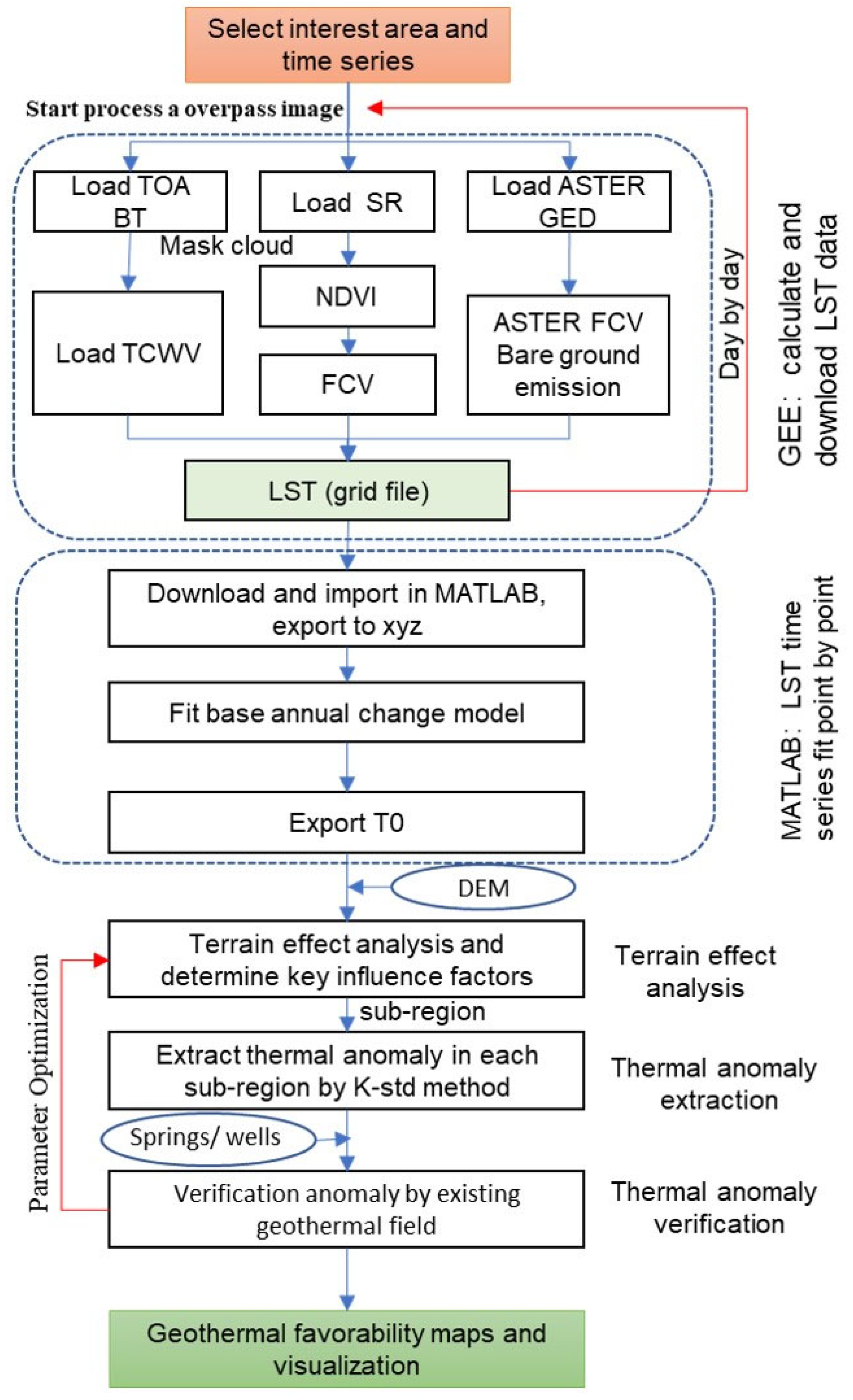
Workflow: The workflow of this study is illustrated in Figure 1. Select study region and time series, retrieve TOA and SR datasets from GEE, calculate NDVI and FCV, compute single-image LST, iterate for full time series, and download. Import LST grids to MATLAB, convert to XYZ, and fit each pixel’s temperature time series to the annual variation model, obtaining T0 for each point. Download high-precision DEM, calculate the aspect, slope, and hillshade, and analyze correlations with T0.

3. Geological Background

The study area is located in the Shanxi Graben System (or northern Fenwei Graben), spanning 110–114°E, 38–41°N. The Shanxi Graben System lies at the transitional zone between the eastern and western blocks of the North China Craton, representing a typical active extensional tectonic zone. The western boundary is the Ordos Basin; the eastern boundary is the Taihang Mountains. The entire Shanxi Graben System comprises a northeast–southwest trending narrow rift valley basin with approximately 2–4 km-thick Cenozoic sediments. The region contains numerous active faults, frequent seismicity, Cenozoic volcanoes, and hot springs. Overall, geothermal resources are abundant. previous studies have identified several geothermal anomaly zones within the Shanxi Graben system, including Taiyuan–Jincheng, Datong–Shuozhou, Xinzhou, Changzhi–Jincheng, Lüliang–Linfen, Yanggao, and Linfen–Yuncheng, as well as multiple rift-related geothermal belts [37,38], particularly in the Weihe Basin, with a long history of geothermal utilization dating to the Qin Dynasty (Huaqing Pool). In recent years, resources have been extensively developed for heating and domestic hot water, with heating coverage exceeding 100 million m². Additionally, the northern region, particularly Datong and Tianzhen, hosts North China’s highest-temperature wells, exceeding 150 °C.

Khutorskoy et al. [39] estimated that the surface heat flow within the Shanxi–Liaohe Rift zone ranges from 75.3 to 79.5 mW/m², which is significantly higher than that of the surrounding mountainous regions (37.7–46.1 mW/m²) and also exceeds the national average heat flow of China (61.5 mW/m²). The Datong Basin is surrounded by densely distributed volcanic edifices, particularly concentrated along major deep-seated fault zones in its southern and peripheral regions [37]. In contrast, volcanic outcrops are relatively sparse in the northeastern part of the basin, especially in the Yanggao–Tianzhen area. This distribution pattern suggests that the region may represent a subsurface magmatic intrusion zone, potentially associated with concealed magma bodies or high-temperature anomalies and thus constitutes a favorable natural setting for geothermal accumulation.

Based on steady-state wellhead temperature measurements, Lu et al. reported an average geothermal gradient of 5.03 °C/100 m. Furthermore, the geothermal gradient increases as the distance to major faults decreases, indicating a strong structural control of subsurface heat transfer and fluid circulation [37].

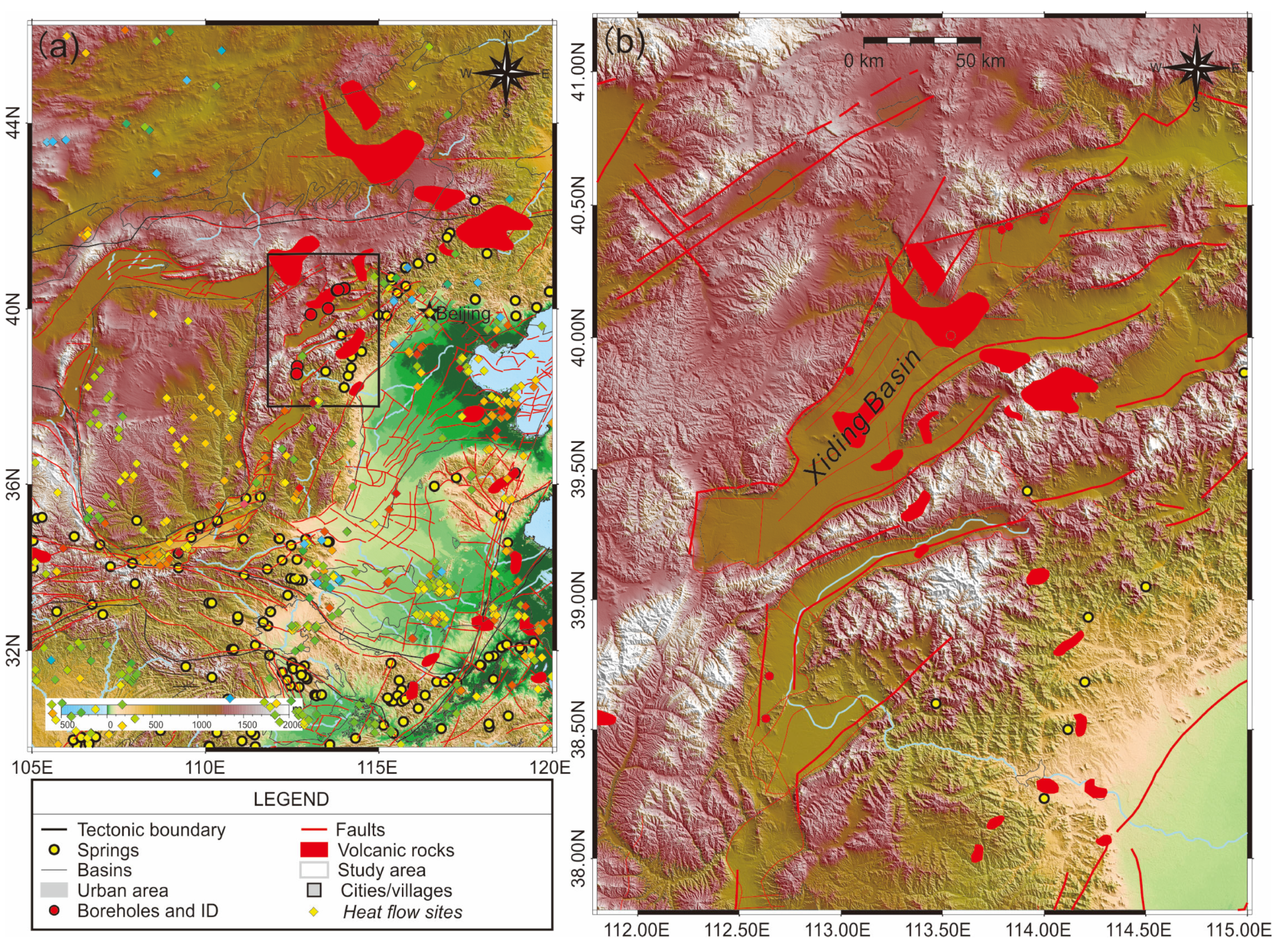
As illustrated in Figure 2, this study focuses on the Xinzhou–Dingxiang Basin and Datong Basin. These basins trend southwest–northeast, representing typical half-graben basins with approximately 1.8 km sediment thickness. The region has enormous geothermal potential, especially for high-temperature resources, making it a recent hotspot for North China geothermal exploration. However, overall exploration remains limited. Thermal infrared remote sensing can provide targeted recommendations and data support for further exploration. Notably, Shanxi Province is a major coal province in China; developing clean geothermal resources is significant for energy structure transformation and achieving carbon neutrality goals.

4. Results and Discussion

4.1. LST Time Series

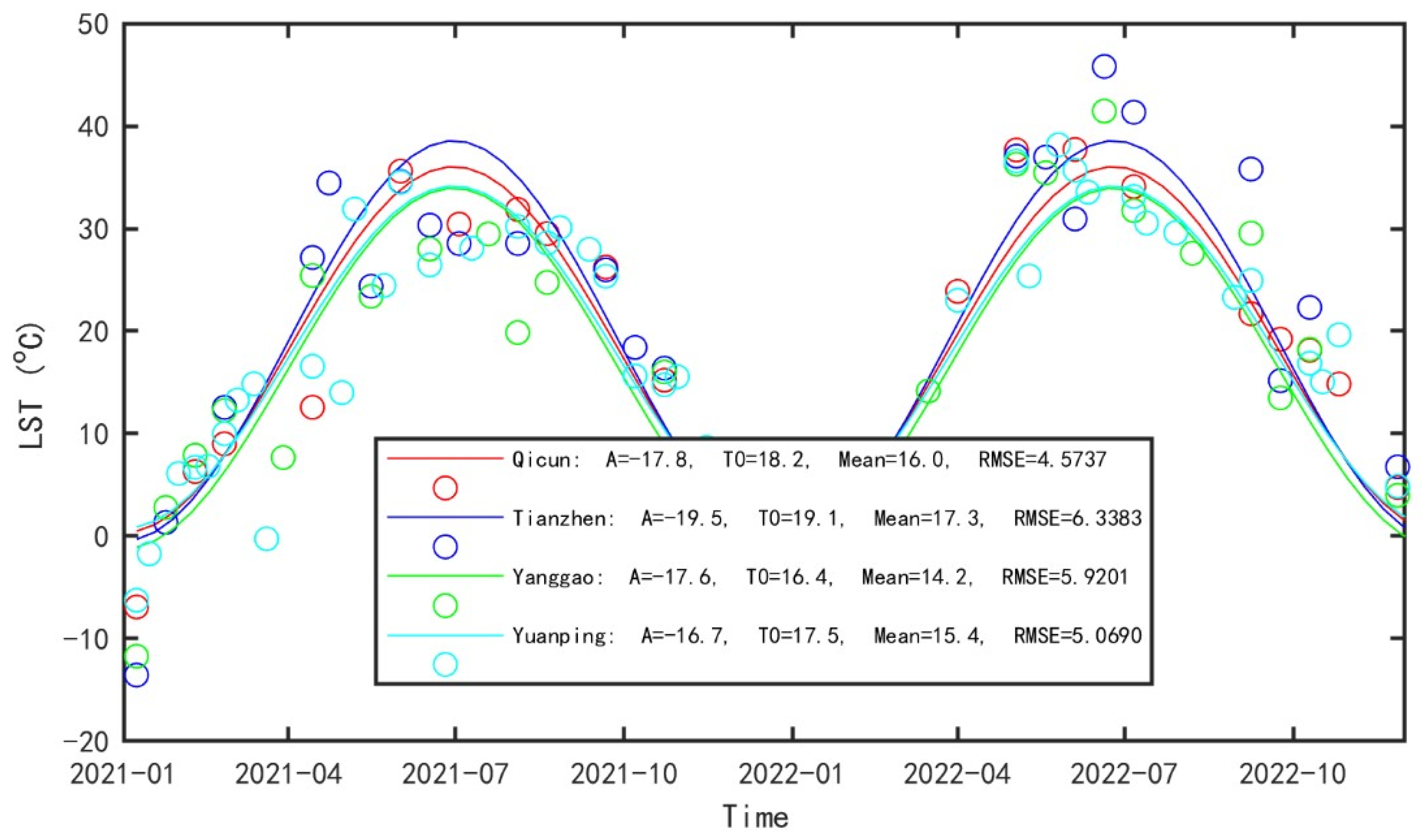
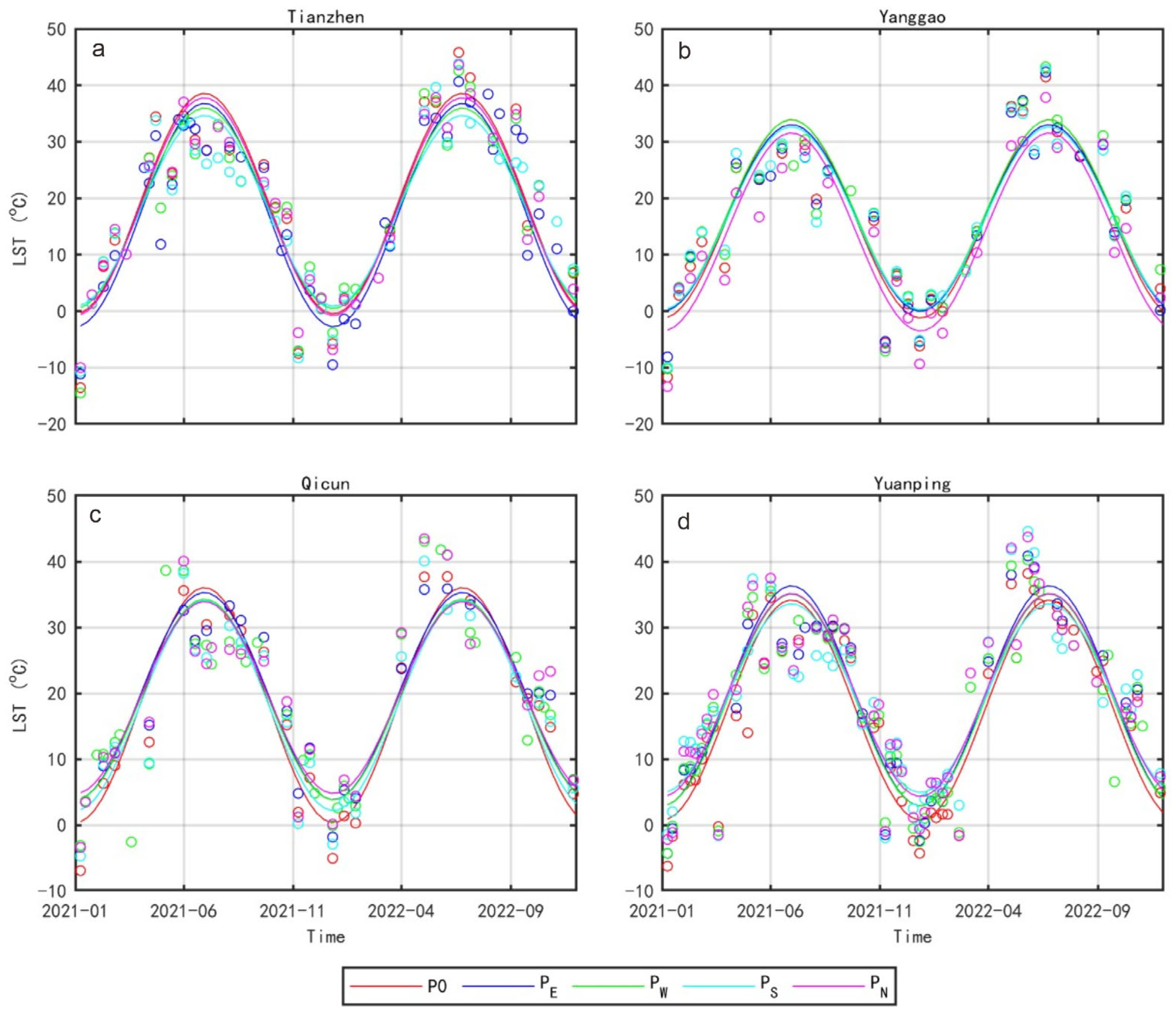
We selected four geothermal sites of interest (Tianzhen, Yanggao, Yuanping, Xinzhou) and calculated temperatures for 30 m buffer zones from 1 January 2021 to 31 December 2022. Valid temperature points generally cover all months, showing clear annual variation: winter minimum ~0 °C, summer maximum ~30 °C, consistent with local multi-year climate data. Based on time series, we calculated annual variation fitting results. As depicted in Figure 3, overall fitting is satisfactory, with residuals of ~5 °C. The main reason is discrete temperature–time sampling: Landsat scans the study area only twice monthly, and cloud cover further reduces valid points. Annual variation model-fitted mean temperatures are generally 2 °C higher than arithmetic means, mainly because winter has less cloud cover (more valid points, higher weight), demonstrating that model-fitted temperatures are more representative (

Table 1. Comparison of arithmetic mean LST and model-fitted background temperature (T0). for four representative geothermal sites in the Shanxi Graben System.

Feature Points	LST
	Annual Average	T0	A	Elevation
Tianzhen	17.32	19.06	19.52	1043
Yanggao	14.17	16.36	17.58	1043
Qicun	16.00	18.20	17.85	833
Yuanping	15.41	17.45	16.70	894

).

After completing the time-series fitting at representative points, the approach was extended to the entire study area. Approximately 10⁶ pixels were processed by applying the annual temperature variation model on a per-pixel basis, yielding the background temperature parameter (T0) and amplitude parameter (A) for each location. Compared with conventional annual mean temperature calculations, T0 is derived from continuous-function fitting to irregularly sampled time-series data, which effectively mitigates biases caused by cloud cover and uneven temporal distribution of observations. As such, it provides a more representative measure of the true land surface thermal background.

More importantly, T0 serves not only as a background temperature indicator for subsequent anomaly detection but also, together with the amplitude parameter A, forms the core basis for geothermal anomaly discrimination. In geothermal anomaly zones, where subsurface heat is continuously transferred to the surface, two characteristic signatures are typically observed: (1) relatively elevated winter temperatures, leading to an increase in T0, and (2) suppressed summer warming due to enhanced groundwater activity and evapotranspiration, resulting in a reduction in A. Therefore, compared with a single temperature metric, the combined analysis of T0 and A is more effective in distinguishing “true geothermal anomalies” from “pseudo-anomalies” induced by topography, land cover, or climatic effects.

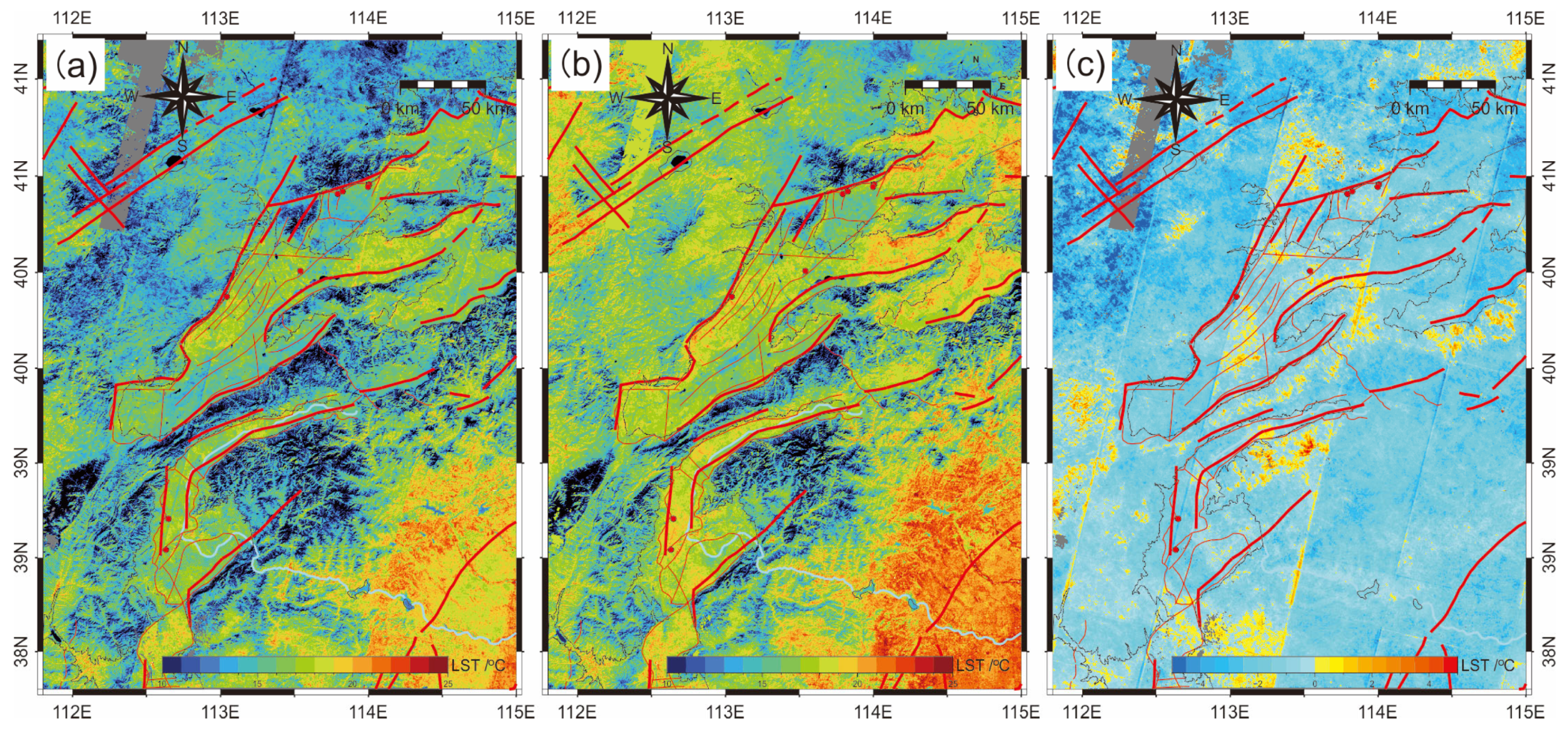
The regional temperature maps reveal a strong topographic control of land surface temperature (LST). High-elevation mountainous areas (e.g., the uplifted flanks of the rift system) exhibit relatively low temperatures, whereas basin and plain regions (e.g., the Xinzhou–Dingxiang Basin, Datong Basin, and parts of the North China Plain) show comparatively higher temperatures. Overall, the rift basins (including the Xinzhou–Dingxiang and Datong basins), the western Ordos Basin, and the southeastern North China Plain are characterized by pronounced positive thermal anomalies, with annual mean temperatures ranging from 20 to 30 °C. In contrast, the Taihang Mountains display clear negative anomalies, with annual mean temperatures of approximately 10 to 20 °C (Figure 4).

4.2. Topographic Effects on LST

Because near-term geothermal utilization prioritizes population centers in low-relief basins, we focus on the Datong and Xinzhou–Dingxiang basins. Basin margins approximately follow the 1200 m contour, which we adopt as a practical boundary for sub-regional partitioning. Within each sub-region, anomaly thresholds are estimated from local LST statistics as mean + 1.5 × SD, improving separation of geothermal anomalies from seasonal or topographic variability.

To minimize the influence of terrain-induced temperature variability, the analysis was restricted to relatively flat areas below the 1200 m elevation contour and with slopes less than 3°. In the study region, elevations above 1200 m are mainly associated with mountainous terrain, where temperature patterns are strongly influenced by elevation lapse rates, slope-induced variations in solar radiation, and terrain shadowing. These factors may produce apparent thermal anomalies unrelated to geothermal processes.

Similarly, restricting the analysis to slopes lower than 3° reduces temperature differences associated with the slope aspect and solar illumination. The flat terrain provides more uniform surface energy balance conditions and improves the reliability of comparisons among pixels.

Sensitivity checks using slightly different thresholds indicate that moderate variations in the elevation and slope criteria do not significantly alter the spatial distribution of the detected anomalies, suggesting that the results are robust to reasonable parameter choices.

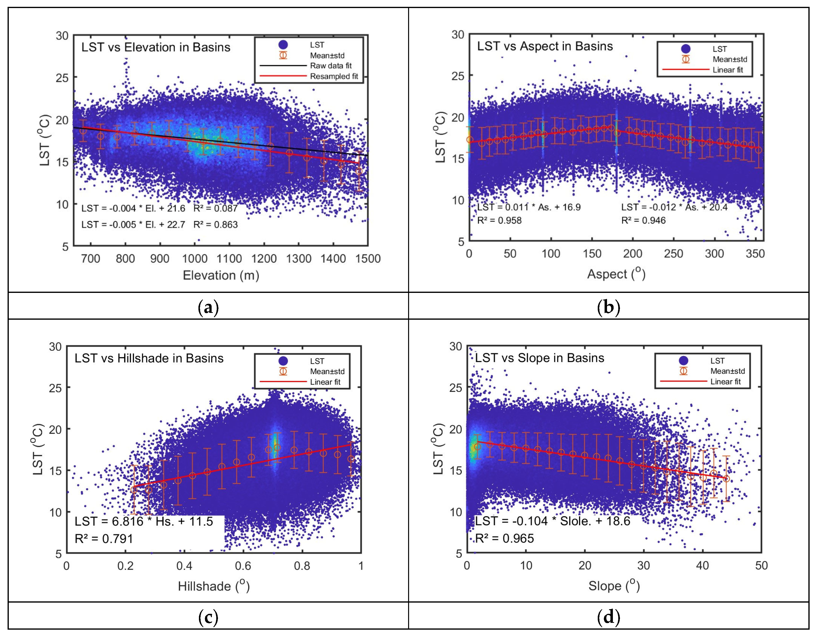
To attenuate terrain-induced bias in LST and better reveal deep thermal signals, we apply sub-regional corrections for the elevation, aspect, slope, and hillshade [16]. Elevation is partitioned into 600–800 m (no correction) and 800–1500 m (corrected); areas > 1500 m are excluded due to sparse samples. The aspect is grouped into 0–165° (positive) and 165–360° (negative) exposure, and slope into 0–4° (positive) and 4–35° (negative), with >35° excluded. Hillshade is used to screen shading effects and stabilize local statistics.

The aspect affects the solar radiation received by surfaces. Landsat scans the study area at ~11:00 local time. Resampling temperatures by 10° aspect bins shows that the aspect–LST relationships follow tight piecewise linear patterns (R² > 0.95) (Figure 5). In the 0–165° range, temperature increases with the aspect; in the 165–360° range, LST decreases with the aspect.

Hillshade correlates positively with LST overall, with data concentrated around 0.7. Slope generally correlates negatively with temperature, but most slopes are 0–3°, indicating flat basin terrain. (For hillshade calculation simplification, we selected mid-March as representative: solar altitude 45°, azimuth 215°. We use these values in subsequent calculations.)

Considering that hillshade is actually a function of the solar zenith, slope, solar azimuth, and aspect—not an independent variable—and that slope correlates strongly with elevation (also not independent), we consider only the elevation and aspect as independent topographic factors in the correlation analysis.

4.3. Known Geothermal Areas and Surrounding Temperature Time Series

Tianzhen, Yanggao, Yuanping, and Xinzhou are four known geothermal sites in the Fenwei Graben (

Table 2. LST parameters for known geothermal anomalies and surrounding reference points.

Site	Water Temperature	Feature Points	LST
			Annual Average	T0	A	Elevation
Tianzhen	100 m 104 °C	P0	17.32	19.06	19.52	1043
		PE	18.04	17.02	19.77	1043
		PW	17.38	18.21	17.75	1043
		PS	17.20	17.76	16.88	1043
		PN	16.63	18.51	19.30	1043
Yanggao	100 m 104 °C	P0	14.82	16.84	16.71	1043
		PE	15.27	16.19	15.79	1043
		PW	14.59	16.20	17.25	1043
		PS	15.35	16.31	16.13	1043
		PN	15.06	16.16	18.23	1226
Qicun	500 m 50 °C	P0	16.00	18.20	17.85	833
		PE	17.40	19.57	15.72	833
		PW	16.42	19.05	15.23	833
		PS	16.10	18.12	15.94	833
		PN	17.48	19.34	14.57	833
Yuanping	300 m 45 °C	P0	15.41	17.45	16.70	894
		PE	18.02	19.62	16.70	894
		PW	16.45	18.98	16.08	894
		PS	16.43	19.25	14.33	894
		PN	17.52	19.73	15.41	894

). Tianzhen and Yanggao reach > 100 °C at a 100 m depth (medium-to-high temperature resources). Yuanping and Xinzhou reach 50 °C at a 500 m depth (low-temperature resources). To study temperature differences between geothermal areas and surroundings, we sampled 30 m buffers at geothermal point centers (P0) and four points 2 km away in cardinal directions (PE, PW, PS, PN) with 30 m buffers. LST results from 2021–2022 show that temperatures vary by −10 to 40 °C, averaging ~25 °C. Temperature data have 16-day intervals (~2 points/month), with fewer summer observations due to cloud cover (Figure 6).

Tianzhen anomaly (T0) vs. surrounding points: temperature range −20~30 °C. In winter, T0 > T1–T4; in summer, it is reversed; spring/autumn show weak patterns. Least-squares fitting shows overall good fit. T0 has a slightly higher background temperature (+1 °C, 3%) and significantly lower amplitude (−2 K, 5%). The fitted temperature is 25 °C vs. the 24 °C direct mean. Of note, currently, only one temperature point confirms the anomaly; the anomaly extent is unclear, so P1–P4 may not represent all background—some may be within the anomaly center.

The Yanggao anomaly (G0), another high-temperature anomaly like Tianzhen, shows similar patterns. However, the northern point (PN) is significantly lower, affected by an elevation increase.

Yuanping, a low-temperature resource with deeper burial, shows no clear LST anomaly. The eastern point (PE) is urban, showing consistently higher temperatures year-round.

4.4. Thermal Anomaly Indicators and Extraction—Elevation Correction and Aspect-Based Sub-Regional Extraction

To better characterize land surface temperature (LST) in the study area, we define the Shanxi Rift Zone (SRZ) as the region of interest and clip all datasets to SRZ. Elevation is grouped into 600–800 m (no correction) and 800–1500 m (corrected), and the aspect is group into 165–360° (negative) and 0–165° (positive).

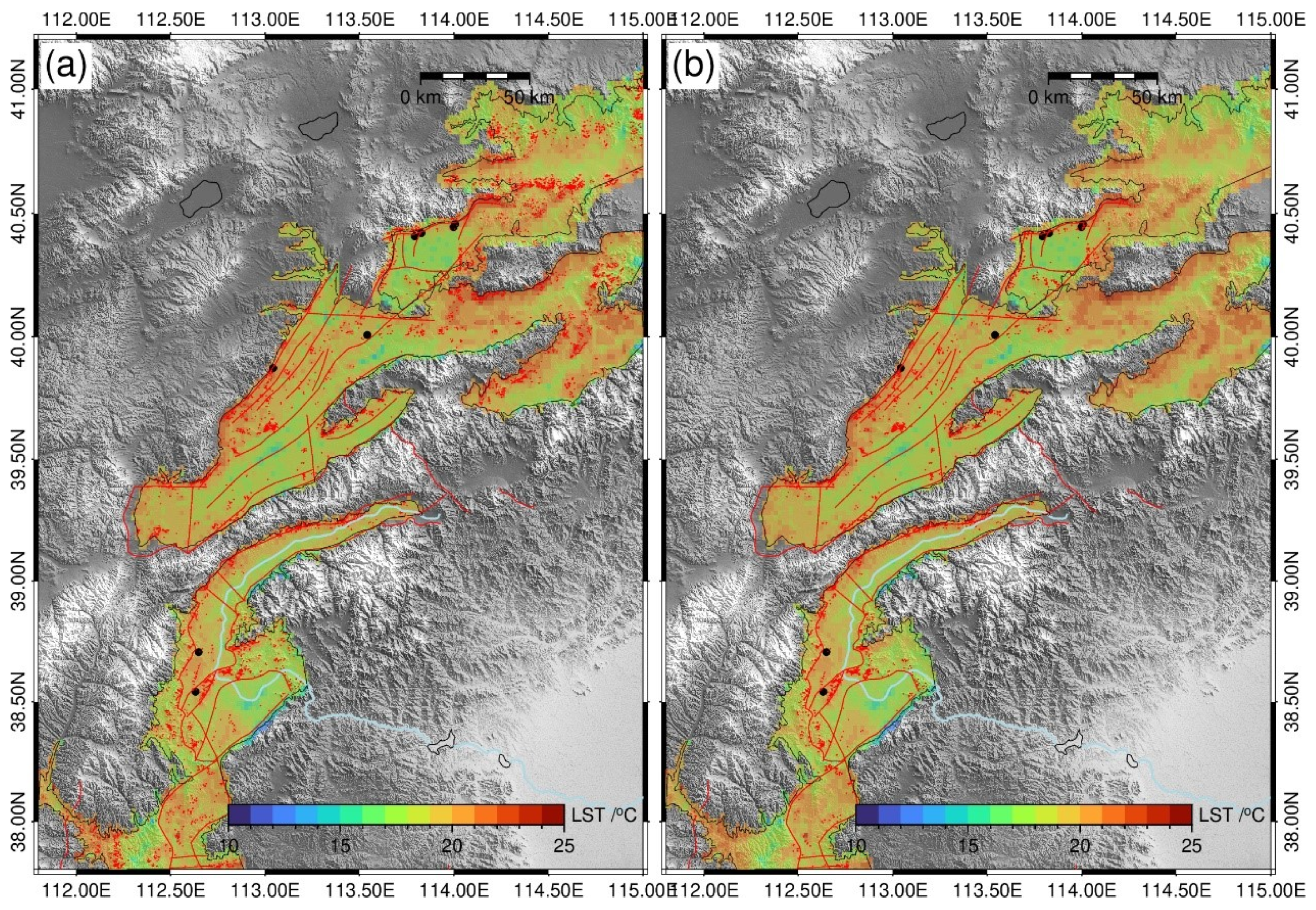
To control elevation and aspect effects, we apply sub-regional thresholding: elevation bins at ΔD = 0.2 are further partitioned by an aspect at ΔAs = 30°. Within each sub-region, the detection threshold is defined as the mean + 1.5 × SD (Figure 7).

Thermal anomalies show a clear association with mapped faults but remain spatially dispersed. Given the strong expected relationship between geothermal manifestations and faults, we apply 5 km buffers around faults and treat anomalies within the buffers as valid geothermal anomalies (Figure 7). The extracted anomalies exhibit good spatial agreement with known geothermal points. Elevation correction is applied.

5. Discussion

5.1. Local Optimum Issues

The nonlinear modeling methods and algorithms used in geothermal resource prediction include nonlinear least-squares, machine learning models (e.g., neural networks, support vector machines, random forests), etc., to capture the complexity and nonlinearity of geothermal systems [40,41].

5.2. Uncertainty and Validation

Sources of uncertainty in geothermal resource prediction include remote sensing data errors, model uncertainties, etc. Validation methods assess model accuracy and reliability, using ground observation data or other independent sources.

Through time-series analysis, LST shows a clear improvement in thermal anomaly identification compared to single-image results (day or night), making high-temperature geothermal signals more significant [15].

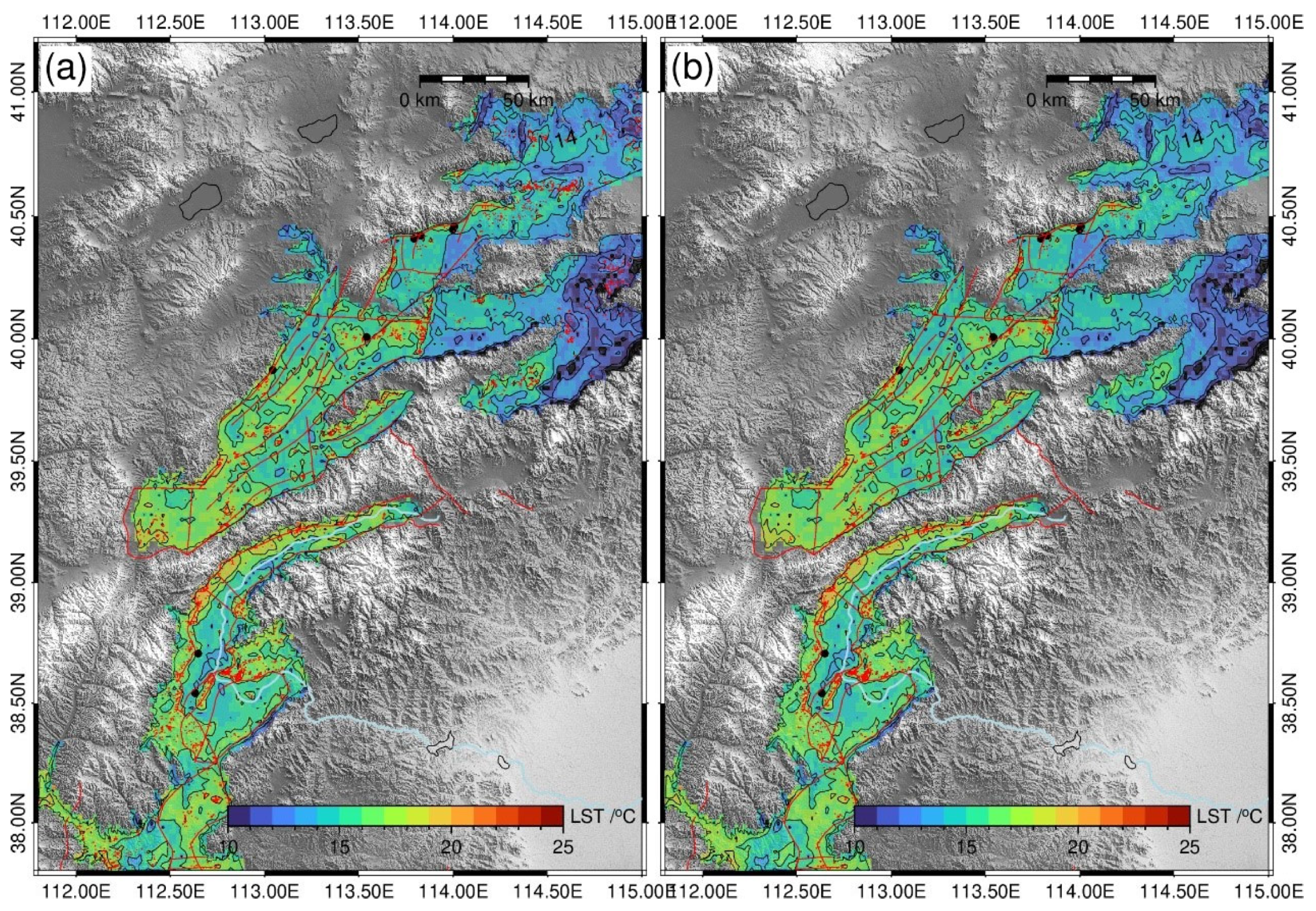
Additionally, it can be observed that a comparison between the historical Landsat 5 dataset (1991–1992) and the recent Landsat 8 dataset (2021–2022) reveals a noticeable increase in thermal anomalies in urbanized regions. In the earlier dataset, thermal anomalies are mainly concentrated along fault-controlled geothermal zones, whereas the recent dataset shows additional high-temperature areas corresponding to expanding urban centers. This pattern suggests that urban heat island effects may partially mask geothermal signals in modern datasets, highlighting the potential value of historical satellite data for geothermal reconnaissance before large-scale urban development.

5.3. Comparison with Alternative Approaches

Our annual temperature variation model approach can be compared with several alternative methodologies recently proposed in the literature:

Multi-Source Data Fusion: Recent studies have explored integrating multiple thermal infrared sources (Landsat, ASTER, MODIS) to increase the temporal sampling density and improve anomaly detection reliability [14]. While this increases data availability, it introduces complexities related to inter-sensor calibration and spatial resolution differences. Our single-sensor time-series approach maintains internal consistency, though at the cost of reduced temporal sampling.

Winter-Summer Contrast Methods: Several researchers have proposed using the winter–summer LST difference as a geothermal indicator, based on the principle that geothermal areas exhibit smaller seasonal variations [15]. Our amplitude parameter A provides a continuous measure of seasonal variation, offering more information than a simple two-season difference. Additionally, the sinusoidal model naturally accounts for variations in cloud-free observation timing across different years.

Machine Learning Approaches: Recent applications of machine learning for geothermal anomaly detection have shown promising results, with Random Forest and XGBoost (v2.0.3) algorithms achieving high classification accuracies when trained on multi-source datasets including thermal, geological, and geophysical features [18]. However, these approaches require substantial training data from known geothermal fields, which may limit their transferability to poorly studied regions. Our physically based model requires no training data and maintains interpretability through its explicit parameters.

Day–Night Thermal Difference: Daytime–nighttime LST differences have been used to reduce solar radiation effects and enhance geothermal signals [15]. While conceptually appealing, this approach is limited by the availability of nighttime thermal observations, which are less frequent and have lower signal-to-noise ratios for Landsat data.

5.4. Detection Depth and Signal Attenuation

The detectability of subsurface geothermal anomalies at the surface depends on the depth, intensity, lateral extent of the heat source, and thermal properties of overlying materials. Theoretical heat conduction models suggest that a geothermal anomaly at depth z produces a surface temperature anomaly ΔT_surface that decays approximately as follows:

$$\mathsf{\Delta }{\mathrm{T}}_{\mathrm{s}\mathrm{u}\mathrm{r}\mathrm{f}\mathrm{a}\mathrm{c}\mathrm{e}}\approx \mathsf{\Delta }{\mathrm{T}}_{\mathrm{s}\mathrm{o}\mathrm{u}\mathrm{r}\mathrm{c}\mathrm{e}}\times \left({\displaystyle \frac{{\mathrm{r}}^2}{{\mathrm{r}}^2+{\mathrm{z}}^2}}\right)$$

(5)

where r is the lateral radius of the heat source and ΔT_source is the temperature anomaly at source depth. This relationship explains why shallow geothermal systems (such as Tianzhen at ~100 m depth) produce detectable surface signatures (1–2 °C), while deeper systems (>500 m) may be undetectable or produce only marginal signals (<0.5 °C) that fall within measurement uncertainty.

Our results confirm this theoretical expectation: high-temperature fields at Tianzhen and Yanggao (100 m depth, >100 °C) show clear thermal anomalies in both T0 and amplitude parameters, while deeper low-temperature systems at Yuanping and Qicun (300–500 m depth, 45–50 °C) show weaker or ambiguous signals. This finding has important implications for exploration strategy: thermal remote sensing is most effective for the reconnaissance of shallow to moderate-depth systems but should be complemented by geophysical methods for deep geothermal exploration.

5.5. Limitations and Uncertainty Sources

Several sources of uncertainty and potential bias affect our results:

Sampling Bias: The 16-day Landsat revisit cycle combined with cloud cover creates irregular temporal sampling, with typically 30–50 usable observations over a 2-year period. Following an integrated evaluation of data availability and cloud cover minimization, the 2021–2022 timeframe was ultimately selected as the monitoring period for this study. this sampling is biased toward clear-sky conditions, which tend to be drier and may not be representative of average conditions. Additionally, summer observations are often underrepresented due to higher cloud cover during the monsoon season, potentially biasing amplitude estimates.

Near-surface wind effects: Near-surface wind fields may influence land surface temperature through convective heat exchange and horizontal advection. Although multi-temporal fitting reduces short-term meteorological variability, wind-induced cooling or warming may still introduce additional uncertainty in the detection of subtle geothermal anomalies.

Applicability: The workflow is designed for tectonically extensional regions where geothermal systems are structurally controlled by faults, such as rift basins and graben systems. However, regional climatic conditions and surface environments may influence the detectability of geothermal signals, and therefore site-specific calibration may be required when applying the method to other geological settings.

Local-Scale Variations: Our 100 m spatial resolution may not fully capture the small-scale thermal anomalies associated with fracture-controlled geothermal systems. Higher-resolution thermal data from airborne or UAV platforms (1–10 m resolution) could potentially identify additional geothermal targets, particularly in structurally complex areas.

Subsurface Hydrology: Our analysis assumes that surface thermal anomalies are primarily driven by conductive heat transfer from depth. However, groundwater flow can significantly modify the shallow geothermal field through coupled convective–conductive heat transfer processes. On the one hand, groundwater acts as an efficient heat carrier, transporting thermal energy from the heat source zone to surrounding areas, which may lead to a lateral displacement of the thermal anomaly center. On the other hand, deep circulation of cold groundwater can reduce shallow heat accumulation through strong convective heat exchange, thereby producing negative surface thermal anomalies and suppressing the upward conduction of heat from the source region.

As the present study lacks an integrated interpretation incorporating hydrogeological data, we have decided to treat this aspect as a priority direction for future research.

Validation Limitations: Our validation is based on four known geothermal sites with variable depths and temperatures. A more comprehensive validation using a larger database of geothermal wells, including both producing and non-productive wells, would provide a more robust assessment of detection accuracy and false-positive rates.

Land Surface Temperature (LST) anomalies can also be induced by various non-geothermal factors, such as urban heat islands and seasonal vegetation dynamics. These interfering factors constitute a major source of uncertainty, as they can alter surface heat capacity and generate pseudo-anomalies that mimic geothermal signals. Our current annual temperature variation model cannot completely isolate deep geothermal heat flux from these complex superficial thermal responses. To address this limitation and further refine the extracted geothermal targets, our future research will combine the current approach with 3D numerical heat-flow modeling, high-resolution land-use masking, and multi-source geophysical surveys.

5.6. Future Research Directions

Sensor Fusion and Improved Temporal Resolution: Combining Landsat 8/9 with other thermal sensors (ASTER, Sentinel-3, ECOSTRESS) could improve temporal sampling and allow for more robust parameter estimation. ECOSTRESS, with its variable overpass times, offers particular potential for capturing the full diurnal cycle, which could be incorporated into an enhanced temperature-variation model.

Three-Dimensional Heat Flow Modeling: The integration of remote sensing results with 3D numerical heat flow models could help estimate the subsurface thermal structure and geothermal potential. Physics-informed machine learning approaches could combine the pattern recognition capabilities of ML with the physical constraints of heat-transfer equations.

Hyperspectral Thermal Sensing: The detection of deeply buried geothermal systems is currently limited when surface thermal anomalies approach the threshold of uncertainty. Future hyperspectral thermal sensors will enable improved emissivity determinations and more accurate LST retrieval, particularly in areas with heterogeneous surface compositions. This could reduce one of the major uncertainty sources in current LST products.

Early Historical Data Analysis: An analysis of early Landsat 5 and 7 thermal data (1980s–2000s) before significant urbanization could help identify geothermal anomalies now masked by urban heat islands, as suggested by our preliminary comparison of 1991–1992 and 2021–2022 results (Figure 8).

Integrated Geothermal Exploration Framework: Combining thermal remote sensing with other remote sensing techniques (InSAR for surface deformation, gravimetry for subsurface density structure, magnetic surveys for magnetic anomalies), geological structural analysis, and machine learning classification could provide a comprehensive geothermal exploration framework suitable for regional-scale reconnaissance.

6. Conclusions

This study demonstrates that physics-based modeling of land surface temperature time series using an annual temperature variation model (T(t) = T0 + A·sin(2πt/τ + φ)) provides an effective approach for geothermal reconnaissance. The main findings and contributions are as follows:

• Method Development: We successfully implemented a nonlinear least-squares fitting approach (Levenberg–Marquardt algorithm) to extract background temperature (T0) and amplitude (A) parameters from irregular, cloud-affected Landsat 8 LST time series. The model-fitted T0 values are systematically ~2 °C higher than simple arithmetic means, reflecting more representative temperatures by accounting for seasonal sampling bias (reduced winter observations due to less cloud cover).
• Topographic Effects: A systematic analysis reveals strong topographic controls based on LST within basin areas (<1200 m elevation): elevation shows −4 °C/100 m gradient above a 800 m elevation; the aspect exhibits tight piecewise linear relationships (R² > 0.95) with opposite trends in 0–165° and 165–360° ranges; the slope and hillshade show weaker, non-independent effects. These results emphasize the critical importance of topographic correction, consistent with recent studies showing 36–45% pseudo-anomaly reduction after proper correction [18].
• Geothermal Detection Performance: Known high-temperature geothermal fields (Tianzhen and Yanggao, >100 °C at 100 m depth) exhibit clear thermal anomalies: elevated T0 (+1–2 °C, 3–5% relative) and reduced amplitude (−2 K, 5–10% relative) compared to surrounding areas. These signatures are consistent with theoretical expectations for shallow geothermal systems. However, deeper low-temperature systems (Yuanping and Qicun, 45–50 °C at 300–500 m depth) show weak or ambiguous signals, indicating fundamental detection limitations for deeply buried resources where surface temperature anomalies fall below uncertainty thresholds (~1.5 K).
• Extraction Strategy: Sub-regional thermal anomaly extraction (elevation and aspect subdivisions) combined with 5 km fault-proximity buffers successfully identifies thermal anomalies spatially correlated with known geothermal sites. This multi-stage filtering approach reduces false positives from topographic effects and urban heat islands, while leveraging the established structural control of geothermal systems.
• Advantages over Conventional Approaches: Compared to simple temporal averaging, the annual variation model (a) better represents background conditions through temporal integration, (b) naturally accounts for irregular sampling by fitting continuous functions, (c) provides amplitude information reflecting seasonal thermal behavior, and (d) enables the separation of geothermal signals from meteorological variations.

Despite the promising performance of the proposed method for shallow geothermal systems, several limitations should be acknowledged. Thermal infrared remote sensing is inherently sensitive to near-surface thermal signals, which limits its ability to detect deeply buried geothermal resources where surface temperature anomalies are weak or absent. In addition, uncertainties in the model fitting process and the limited availability of validation sites may influence the robustness of the results. Future studies incorporating more extensive geothermal datasets and improved uncertainty treatment could further enhance the reliability of the method.Future research should focus on improving temporal coverage through the integration of multi-sensor thermal datasets and developing more advanced analytical frameworks that combine thermal remote sensing with other geophysical and geological information. In addition, emerging approaches such as machine learning and high-resolution thermal observations may further improve the detection and interpretation of geothermal-related thermal anomalies.

References

1. Muffler, L.J.P. Assessment of Geothermal Resources of the United States—1978; Geological Survey; US Department of the Interior: Washington, DC, USA, 1979; Volume 790. [Google Scholar]
2. Okoroafor, E.R.; Smith, C.M.; Ochie, K.I.; Nwosu, C.J.; Gudmundsdottir, H.; Aljubran, J.M. Machine Learning in Subsurface Geothermal Energy: Two Decades in Review. Geothermics 2022, 102, 102401. [Google Scholar] [CrossRef] [Scilit]
3. Gutiérrez-Negrín, L.C.A. Evolution of Worldwide Geothermal Power 2020–2023. Geotherm. Energy 2024, 12, 14. [Google Scholar] [CrossRef] [Scilit]
4. Simiyu, S.M. Application of Micro-Seismic Methods to Geothermal Exploration: Examples from the Kenya Rift. In Proceedings of the Short Course VIII on Exploration for Geothermal Resources, Lake Naivasha, Kenya, 31 October–23 November 2009; UNU-GTP: Reykjavik, Iceland, 2009; p. 31. [Google Scholar]
5. Yalcin, M.; Kilic Gul, F.; Yildiz, A.; Polat, N.; Basaran, C. The Mapping of Hydrothermal Alteration Related to the Geothermal Activities with Remote Sensing at Akarcay Basin (Afyonkarahisar), Using Aster Data. Arab. J. Geosci. 2020, 13, 1166. [Google Scholar] [CrossRef] [Scilit]
6. Silvestri, M.; Marotta, E.; Buongiorno, M.F.; Avvisati, G.; Belviso, P.; Bellucci Sessa, E.; Caputo, T.; Longo, V.; De Leo, V.; Teggi, S. Monitoring of Surface Temperature on Parco Delle Biancane (Italian Geothermal Area) Using Optical Satellite Data, UAV and Field Campaigns. Remote Sens. 2020, 12, 2018. [Google Scholar] [CrossRef] [Scilit]
7. Gemitzi, A.; Dalampakis, P.; Falalakis, G. Detecting Geothermal Anomalies Using Landsat 8 Thermal Infrared Remotely Sensed Data. Int. J. Appl. Earth Obs. Geoinf. 2021, 96, 102283. [Google Scholar] [CrossRef] [Scilit]
8. Sun, J.; Liu, K.; He, Q.; Yu, T.; Deng, Y. Thermal Infrared Remote Sensing and Soil Gas Radon for Detecting Blind Geothermal Area. Geothermics 2022, 105, 102534. [Google Scholar] [CrossRef] [Scilit]
9. Weldeyohannes, T.T.; Hailu, B.T.; Muluneh, A.A.; Kidane, T. Detection of Geothermal Anomalies in the Northern Lake Abaya Geothermal Field, Main Ethiopian Rift. J. Volcanol. Geotherm. Res. 2022, 430, 107638. [Google Scholar] [CrossRef] [Scilit]
10. Idi, B.Y.; Maiha, A.I.; Abdullahi, M. Spatial Mapping and Monitoring Thermal Anomaly and Radiative Heat Flux Using Landsat-8 Thermal Infrared Data -A Case Study of Lamurde Hot Spring, Upper Part of Benue Trough, Nigeria. J. Appl. Geophys. 2022, 203, 104654. [Google Scholar] [CrossRef] [Scilit]
11. Li, X.; Jiang, G.; Tang, X.; Zuo, Y.; Hu, S.; Zhang, C.; Wang, Y.; Wang, Y.; Zheng, L. Detecting Geothermal Anomalies Using Multi-Temporal Thermal Infrared Remote Sensing Data in the Damxung–Yangbajain Basin, Qinghai–Tibet Plateau. Remote Sens. 2023, 15, 4473. [Google Scholar] [CrossRef] [Scilit]
12. Chen, Z.; Grasby, S.E.; Yuan, W.; Liu, X. Ground Surface Temperature Monitoring Data Analysis and Applications to Geothermal Exploration in Volcanic Areas, Mount Meager, Western Canada. Geothermics 2023, 108, 102610. [Google Scholar] [CrossRef] [Scilit]
13. Romaguera, M.; Vaughan, R.G.; Ettema, J.; Izquierdo-Verdiguier, E.; Hecker, C.A.; van der Meer, F.D. Detecting Geothermal Anomalies and Evaluating LST Geothermal Component by Combining Thermal Remote Sensing Time Series and Land Surface Model Data. Remote Sens. Environ. 2018, 204, 534–552. [Google Scholar] [CrossRef] [Scilit]
14. Chao, J.; Zhao, Z.; Xu, S.; Lai, Z.; Liu, J.; Zhao, F.; Yang, H.; Chen, Q. Geothermal Target Detection Integrating Multi-Source and Multi-Temporal Thermal Infrared Data. Ore Geol. Rev. 2024, 167, 105991. [Google Scholar] [CrossRef] [Scilit]
15. Wang, K.; Jiang, Q.; Yu, D.; Yang, Q.; Wang, L.; Han, T.; Xu, X. Detecting Daytime and Nighttime Land Surface Temperature Anomalies Using Thermal Infrared Remote Sensing in Dandong Geothermal Prospect. Int. J. Appl. Earth Obs. Geoinf. 2019, 80, 196–205. [Google Scholar] [CrossRef] [Scilit]
16. Peng, X.; Wu, W.; Zheng, Y.; Sun, J.; Hu, T.; Wang, P. Correlation Analysis of Land Surface Temperature and Topographic Elements in Hangzhou, China. Sci. Rep. 2020, 10, 10451. [Google Scholar] [CrossRef] [Scilit] [PubMed]
17. Li, Z.-L.; Wu, H.; Duan, S.-B.; Zhao, W.; Ren, H.; Liu, X.; Leng, P.; Tang, R.; Ye, X.; Zhu, J.; et al. Satellite Remote Sensing of Global Land Surface Temperature: Definition, Methods, Products, and Applications. Rev. Geophys. 2023, 61, e2022RG000777. [Google Scholar] [CrossRef] [Scilit]
18. Dong, B.; Li, B.; Song, R.; Chen, H.; Wang, Y. Detection and Constraints of Geothermal Latent Heat Zones under the Complex Terrain of the Western Sichuan Plateau: A Fusion of Multi-Source Temporal Remote Sensing Data. Geothermics 2025, 130, 103287. [Google Scholar] [CrossRef] [Scilit]
19. Coolbaugh, M.F.; Kratt, C.; Fallacaro, A.; Calvin, W.M.; Taranik, J.V. Detection of Geothermal Anomalies Using Advanced Spaceborne Thermal Emission and Reflection Radiometer (ASTER) Thermal Infrared Images at Bradys Hot Springs, Nevada, USA. Remote Sens. Environ. 2007, 106, 350–359. [Google Scholar] [CrossRef] [Scilit]
20. Qin, Z.-H.; Zhang, M.-H.; Karnieli, A.; Berliner, P. Mono-Window Algorithm for Retrieving Land Surface Temperature from Landsat TM6 Data. Dili Xuebao Acta Geogr. Sin. 2001, 56, 456–466. [Google Scholar]
21. Qin, Q.; Zhang, N.; Nan, P.; Chai, L. Geothermal Area Detection Using Landsat ETM+ Thermal Infrared Data and Its Mechanistic Analysis—A Case Study in Tengchong, China. Int. J. Appl. Earth Obs. Geoinf. 2011, 13, 552–559. [Google Scholar] [CrossRef] [Scilit]
22. Li, Z.-L.; Tang, B.-H.; Wu, H.; Ren, H.; Yan, G.; Wan, Z.; Trigo, I.F.; Sobrino, J.A. Satellite-Derived Land Surface Temperature: Current Status and Perspectives. Remote Sens. Environ. 2013, 131, 14–37. [Google Scholar] [CrossRef] [Scilit]
23. Ermida, S.L.; Soares, P.; Mantas, V.; Göttsche, F.-M.; Trigo, I.F. Google Earth Engine Open-Source Code for Land Surface Temperature Estimation from the Landsat Series. Remote Sens. 2020, 12, 1471. [Google Scholar] [CrossRef] [Scilit]
24. Carslaw, H.S.; Jaeger, J.C. Conduction of Heat in Solids; Oxford University Press: Oxford, UK, 1980. [Google Scholar]
25. Bechtel, B. Robustness of Annual Cycle Parameters to Characterize the Urban Thermal Landscapes. IEEE Geosci. Remote Sens. Lett. 2012, 9, 876–880. [Google Scholar] [CrossRef] [Scilit]
26. North, J.S.; Schliep, E.M.; Wikle, C.K. On the Spatial and Temporal Shift in the Archetypal Seasonal Temperature Cycle as Driven by Annual and Semi-Annual Harmonics. Environmetrics 2021, 32, e2665. [Google Scholar] [CrossRef] [Scilit]
27. Shen, H.; Huang, L.; Zhang, L.; Wu, P.; Zheng, C. Long-Term and Fine-Scale Satellite Monitoring of the Urban Heat Island Effect by the Fusion of Multi-Temporal and Multi-Sensor Remote Sensed Data: A 26-Year Case Study of the City of Wuhan in China. Remote Sens. Environ. 2016, 172, 109–125. [Google Scholar] [CrossRef] [Scilit]
28. Marquardt, D.W. An Algorithm for Least-Squares Estimation of Nonlinear Parameters. J. Soc. Ind. Appl. Math. 1963, 11, 431–441. [Google Scholar] [CrossRef] [Scilit]
29. Ma, J.; Shen, H.; Wu, P.; Wu, J.; Gao, M.; Meng, C. Generating Gapless Land Surface Temperature with a High Spatio-Temporal Resolution by Fusing Multi-Source Satellite-Observed and Model-Simulated Data. Remote Sens. Environ. 2022, 278, 113083. [Google Scholar] [CrossRef] [Scilit]
30. Barsi, J.A.; Schott, J.R.; Hook, S.J.; Raqueno, N.G.; Markham, B.L.; Radocinski, R.G. Landsat-8 Thermal Infrared Sensor (TIRS) Vicarious Radiometric Calibration. Remote Sens. 2014, 6, 11607–11626. [Google Scholar] [CrossRef] [Scilit]
31. Sobrino, J.A.; Jiménez-Muñoz, J.C.; Paolini, L. Land Surface Temperature Retrieval from LANDSAT TM 5. Remote Sens. Environ. 2004, 90, 434–440. [Google Scholar] [CrossRef] [Scilit]
32. Dash, P.; Göttsche, F.; Olesen, F.; Fischer, H. Land Surface Temperature and Emissivity Estimation from Passive Sensor Data: Theory and Practice-Current Trends. Int. J. Remote Sens. 2002, 23, 2563–2594. [Google Scholar] [CrossRef] [Scilit]
33. Weng, Q. Thermal Infrared Remote Sensing for Urban Climate and Environmental Studies: Methods, Applications, and Trends. ISPRS J. Photogramm. Remote Sens. 2009, 64, 335–344. [Google Scholar] [CrossRef] [Scilit]
34. Brown, S.; Rodi, W.L.; Seracini, M.; Gu, C.; Fehler, M.; Faulds, J.; Smith, C.M.; Treitel, S. Bayesian Neural Networks for Geothermal Resource Assessment: Prediction with Uncertainty. arXiv 2022, arXiv:2209.15543. [Google Scholar]
35. Han, D.; Liang, X.; Currell, M.; Song, X.; Chen, Z.; Jin, M.; Liu, C.; Han, Y. Environmental Isotopic and Hydrochemical Characteristics of Groundwater Systems in Daying and Qicun Geothermal Fields, Xinzhou Basin, Shanxi, China. Hydrol. Process. 2010, 24, 3157–3176. [Google Scholar] [CrossRef] [Scilit]
36. Lu, Z.; Yang, Y.; Mo, Y.; Liao, H.; Cai, Y. Investigation and Evaluation of Geothermal Resources in Northern Shanxi Province, China. Energies 2025, 18, 1494. [Google Scholar] [CrossRef] [Scilit]
37. Yan, X.; Wei, S.; Zhang, W.; Liu, F.; Liao, Y. Reservoirs and Hydrogeochemical Characterizations of the Yanggao Geothermal Field in Shanxi Province, China. Water 2024, 16, 669. [Google Scholar] [CrossRef] [Scilit]
38. Khutorskoy, M.D.; Teveleva, E.A. Heat Flow in Continental Rift Zones: A New Approach to Data Interpretation. Volcanol. Seismol. 2024, 18, 236–250. [Google Scholar] [CrossRef] [Scilit]
39. Noorollahi, Y.; Itoi, R.; Fujii, H.; Tanaka, T. GIS Integration Model for Geothermal Exploration and Well Siting. Geothermics 2008, 37, 107–131. [Google Scholar] [CrossRef] [Scilit]
40. Mudunuru, M.K.; Ahmmed, B.; Rau, E.; Vesselinov, V.V.; Karra, S. Machine Learning for Geothermal Resource Exploration in the Tularosa Basin, New Mexico. Energies 2023, 16, 3098. [Google Scholar] [CrossRef] [Scilit]
41. Mia, M.d.B.; Nishijima, J.; Fujimitsu, Y. Exploration and Monitoring Geothermal Activity Using Landsat ETM+images: A Case Study at Aso Volcanic Area in Japan. J. Volcanol. Geotherm. Res. 2014, 275, 14–21. [Google Scholar] [CrossRef] [Scilit]
Figure 1. Workflow for geothermal anomaly extraction from Landsat 8 LST based on annual temperature variation model (TOA BT: Top of Atmosphere Brightness Temperature; SR: Surface Reflectance; TCVW: Total Column Water Vapor; NDVI: Normalized Difference Vegetation Index; FCV: Fractional Vegetation Cover; ASTER: Advanced Spaceborne Thermal Emission and Reflection Radiometer; ASTER GED: ASTER Global Emissivity Dataset; LST: Land Surface Temperature; DEM: Digital Elevation Model; K-std method: K-standard deviation method).
Remotesensing 18 01362 g001
Figure 2. Geological tectonic background and topographic map of the study area. (a) Regional overview of tectonic structures, volcanic rocks, and heat flow sites across northern China, with the black rectangle indicating the study area. (b) Enlarged view of major faults and volcanic rocks within and around the Xiding Basin.
Remotesensing 18 01362 g002
Figure 3. Land surface temperature time series and annual variation fitting results.
Remotesensing 18 01362 g003
Figure 4. (a) Annual mean temperature, (b) fitted T0 temperature, and (c) meanfitted difference for 2021–2022.
Remotesensing 18 01362 g004
Figure 5. Correlations between LST and topographic factors: (a) elevation, (b) aspect, (c) hillshade, and (d) slope.
Remotesensing 18 01362 g005
Figure 6. Temperature–time series for known thermal anomalies and surroundings (2021–2022): (a) Tianzhen, (b) Yanggao, (c) Qicun, (d) Yuanping. Comparison of mean values and T0 values.
Remotesensing 18 01362 g006
Figure 7. Thermal anomalies in the Shanxi Rift Zone: (a) anomaly map; (b) anomalies within 5 km of fault buffer zones (2021–2022, Landsat 8).
Remotesensing 18 01362 g007
Figure 8. (a) Shanxi Rift thermal anomaly map, (b) thermal anomalies within 5 km fault buffer zones (1991–1992 from Landsat 5).
Remotesensing 18 01362 g008