Article

The 2025 Mw 5.8 Aheqi Earthquake, China: Blind-Thrust Rupture on an Orogen Basin Boundary Fault from InSAR Observations

School of Geoscience and Info-Physics, Central South University, Changsha 410083, China
*
Author to whom correspondence should be addressed.
Remote Sens. 2026, 18(7), 1078; https://doi.org/10.3390/rs18071078
Submission received: 25 February 2026 / Revised: 30 March 2026 / Accepted: 31 March 2026 / Published: 3 April 2026
(This article belongs to the Special Issue Advances in Remote Sensing for Earthquake and Fault Detection)

Highlights

What are the main findings?
  • The coseismic deformation field of the 2025 Mw 5.8 Aheqi earthquake is clearly obtained from InSAR data after tropospheric delay mitigation, showing maximum uplift of approximately 5.0 cm and 6.0 cm in the ascending and descending tracks, respectively, and indicating a thrust faulting mechanism.
  • Bayesian inversion of InSAR data for the Aheqi earthquake reveals two possible fault models: a south-dipping back-thrust or a north-dipping thrust; the latter is preferred based on an integrated analysis of structural development conditions, surface deformation patterns, and local topography. The preferred fault model was loaded by >2 bar of Coulomb stress from the 2024 Wushi earthquake.
What are the implications of the main findings?
  • The dip ambiguity in the InSAR modeling of the Aheqi earthquake underscores that InSAR-based geometric solutions for moderate blind-thrust earthquakes necessitate the integration of structural and geomorphic analyses.
  • Sequential rupture potential between reactivated and present-day active structures is evidenced by Coulomb stress loading between the geometrically distinct 2024 Wushi and 2025 Aheqi earthquakes, necessitating updated hazard models for southern Tianshan orogen.

Abstract

On 4 December 2025, nearly two years after the 2024 Mw 7.0 Wushi earthquake, an Mw 5.8 event struck the nearby county of Aheqi, southwestern Tianshan. Owing to the subparallel strikes of both nodal planes and the interspersed hypocenter locations among regional structures in the reported focal mechanisms, the exact fault geometry of this event remains unresolved, impeding a better understanding of regional tectonic activity and the associated seismic hazards. To resolve this, we applied Interferometric Synthetic Aperture Radar (InSAR) technique to map the coseismic deformation and invert for the fault geometry and slip pattern. Significant tropospheric delays are mitigated using a moving-window linear model and a multi-interferogram weighted averaging strategy. The result shows significant uplift (~5.0 cm for ascending track and ~6.0 cm for descending track), indicating thrust-dominated mechanism. Bayesian inversion reveals two possible fault models: a 31.6° north-dipping blind thrust or a 54.4° south-dipping back-thrust. While both fault planes fit the InSAR observations, integrated evidence from the absence of back-thrust development conditions, the surface deformation pattern, and regional topography indicates that the north-dipping Aheqi fault is the causative structure. Together with the steeper Maidan fault to the north, it forms the Orogen Basin boundary along the southern Tianshan piedmont. Our findings highlight that resolving moderate blind-thrust seismogenic structures using InSAR requires integration with pre-existing structural and geomorphic evidence. Furthermore, Coulomb stress calculations indicate a rupture-promoting effect from the Wushi earthquake, which occurred on a reactivated fault, onto the Aheqi event, with stress loading exceeding 2 bar at the hypocenter. Thus, the potential for stress-driven sequential rupture between reactivated and present-day active structures necessitates an updated seismic hazard assessment in the southern Tianshan.

1. Introduction

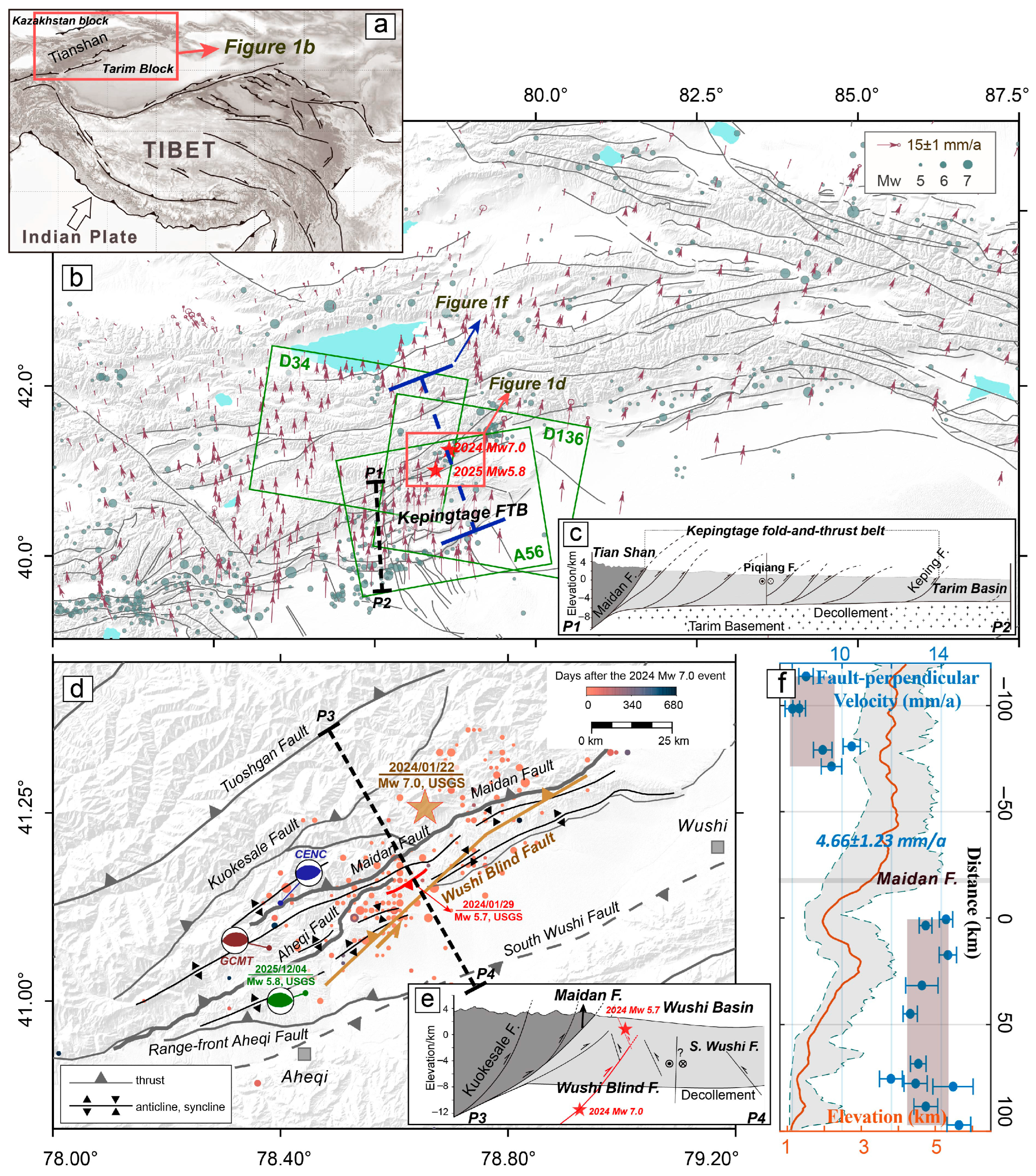
Under the far-field stress transmitted by the ongoing India-Eurasia convergence and confined by the nearly rigid Tarim and Kazakhstan blocks, the Tianshan region undergoes distributed crustal shortening and thickening, developing into one of the largest and actively deforming intracontinental orogenic belts (Figure 1a,b) [1,2,3]. Global Navigation Satellite System (GNSS) measurements reveal a maximum crustal shortening rate of ~20 mm/a between the Pamir and western Tianshan, accounting for approximately half of the India-Eurasia convergence rate (Figure 1b) [4,5,6]. The shortening rate decreases progressively eastward, from ~10–20 mm/a in the western Tianshan (~75.3–82.7°E) to ~5–10 mm/a in the central Tianshan (~82.7–87.6°E), and further diminishes to ~4 mm/a or less in the eastern Tianshan (~87.6–94.8°E) [7]. This deformation is primarily accommodated by a series of nearly east–west trending thrust faults with sinistral strike–slip components, supplemented by conjugate northwest-trending dextral structures [7,8,9,10]. The resulting strain accumulation has generated over 100 strong-to-major earthquakes (Mw ≥ 6) since 1700, including the recent Mw 7.0 Wushi earthquake (22 January 2024, UTC time) in the southwestern Tianshan that caused three fatalities (Figure 1b,d) [11,12,13]. The seismogenic zone and its surrounding areas exhibit significant topographic variations of ~2 km, with a pronounced shortening rate of 4.66 ± 1.23 mm/a derived from GNSS cross-fault profile analysis (Figure 1f).
The Wushi earthquake ruptured a blind, moderately dipping transpressional fault, known as the Wushi blind fault or the south Maidan fault, with its aftershock sequence further illuminating the regional structural complexity (Figure 1d) [12,14,15,16]. Satellite imagery and field investigations revealed surface rupture from an Mw 5.7 aftershock that occurred seven days after the mainshock (29 January 2024) [16,17,18]. Integrated analysis of Interferometric Synthetic Aperture Radar (InSAR) observations and relocated seismicity identified the seismogenic structure as a southeast-dipping back-thrust (hypocentral depth ~1–2 km) within the cover layer above decollement, forming a pop-up structure with the Wushi blind fault (Figure 1d,e) [12,16,19]. The shallow depth of this aftershock is attributed to rupture along a pre-existing weak structure, driven by highly localized stress concentration from mainshock. Furthermore, significant aftershocks clustered along multiple steeply dipping secondary faults that obliquely intersect the rupture plane of the mainshock [19]. These findings highlight a complex fault network and associated rupture hazards in the South Tianshan orogenic belt.
On 4 December 2025, an Mw 5.8 earthquake occurred 24 km southwest of the Wushi earthquake, striking Aheqi County (78.40°E, 41.13°N) in the Kizilsu Kirghiz Autonomous Prefecture, Xinjiang, at a focal depth of ~10 km (Table 1; hereafter referred to as the Aheqi earthquake). Reported focal mechanism solutions from various institutions consistently indicate that the Aheqi earthquake is a thrust-dominated event with minor strike–slip components (Table 1). The USGS and CENC solutions show good agreement, suggesting either a moderate southeast-dipping nodal plane with sinistral motion, or a moderate northeast/north-dipping nodal plane with dextral motion. In contrast, the GCMT solution presents two distinct possibilities: a northwest-dipping sinistral fault or a southwest-dipping dextral fault. The south-dipping plane solutions generally exhibit slightly steeper angles than the north-dipping plane solutions. Moreover, although hypocenter locations from different institutions are separated by less than 9 km from their nearest neighbors, their positions are interspersed among multiple subparallel faults within the complex fault system (Figure 1d). The CENC hypocenter is located north of the Maidan fault, while that from GCMT lies between the Maidan fault and the Aheqi fault, and the USGS location is positioned between the Aheqi fault and the range-front Aheqi fault (Figure 1d). This structural complexity poses significant challenges for the precise identification of the seismogenic fault.
The 2024 Mw 7.0 Wushi earthquake and the 2025 Mw 5.8 Aheqi earthquake both occurred in the hinterland of the Kepingtage fold-and-thrust belt (FTB). This FTB comprises a series of east–west-trending thrust faults and associated anticlines [8,20], which have propagated southward from the orogenic belt toward the Tarim basin along a uniform decollement (Figure 1c). Structurally, its front (near the Tarim basin) is characterized by thin-skinned structure, where active structures are mainly developed within the sedimentary cover above the decollement, while the root (near the Tianshan orogen) exhibits thick-skinned basement-involved structure [20]. The depth of the decollement increases northward from approximately 5 km at the frontal edge to about 10 km in the root zone (Figure 1c) [8,21,22]. Over the past 30 years, more than ten moderate earthquakes (M5.5–6.5) have been recorded in this belt, most of which occurred within its sedimentary cover. This pattern suggests that elastic strain in the Kepingtage FTB is primarily released through frequent moderate earthquakes rather than large events [11,21,22]. The 2024 Mw 7.0 Wushi earthquake represents a notable departure from this pattern, as it ruptured through both the upper sedimentary cover and the underlying basement, with the rupture extending to depths greater than 20 km (Figure 1e) [15,19]. Therefore, the recent 2025 Mw 5.8 Aheqi earthquake provides a valuable opportunity to further investigate the seismogenic mechanisms of this complex transition zone.
Over recent decades, InSAR technique has demonstrated exceptional capability in constraining fault geometry and kinematic characteristics of seismogenic structures in complex tectonic settings, particularly for earthquakes lacking surface rupture [23,24,25,26,27]. By capturing continuous coseismic deformation fields and integrating dislocation modeling with advanced optimization algorithms (e.g., simulated annealing or Bayesian inversion), InSAR enables robust fault parameter determination even in orogenically active regions with intricate fault networks [28,29,30,31].
In this study, we aim to investigate the seismogenic fault of the 2025 Mw 5.8 Aheqi earthquake using coseismic deformation fields derived from ascending and descending Sentinel-1A SAR data. Tropospheric delays in InSAR observations are corrected using a moving-window approach for elevation-dependent atmospheric effects combined with multi-interferogram (four interferograms per track) averaging to reduce stochastic turbulent atmospheric noise. We determine the optimal fault geometries for both north-dipping and south-dipping scenarios through Bayesian inversion, then resolve the distributed slip on the fault plane using the steepest descent algorithm. To further determine the more plausible fault dip, we integrate these results with a comprehensive analysis of regional pre-existing structures, the surface deformation pattern, and topographic changes. Additionally, we analyze the stress perturbation from the Wushi earthquake on the Aheqi event. Finally, we discuss the tectonic implications of the identified seismogenic structure and its seismic hazard significance in the southern Tianshan orogen.
Figure 1. Tectonic setting of the seismogenic region of the 2025 Mw 5.8 Aheqi earthquake. (a) Configuration of the India-Eurasia collision zone showing the location of Tianshan. (b) GNSS velocity field in the Tianshan region with respect to the Eurasian reference frame [32]. The dots denote earthquakes with M ≥ 5 from the USGS catalog (1900–2025). Green rectangular frames with orbit numbers show the coverage of SAR images used in this study. The black line P1–P2 marks the profile location displayed in subfigure (c). The red rectangle outlines the area shown in subfigure (d). The blue line corresponds to the location of the GNSS velocity profile in subfigure (f). (c) Cross-section of the Kepingtage FTB [20]. (d) Distribution of the 2024 Wushi earthquake and aftershocks (22 January 2024–4 December 2025), showing the Wushi blind fault [12] and a back-thrust aftershock fault [15]. The black line P3–P4 marks the profile location shown in subfigure (e). (e) Cross-section of the seismogenic zone [19]. (f) Present-day shortening rate across the seismogenic zone derived from GNSS profile analysis. Blue dots with error bars represent fault-perpendicular velocities and their uncertainties. The brown solid line and flanking dashed lines denote the mean elevation and elevation variation range along the profile, respectively. The shortening rate is estimated from the velocity difference between the averaged rates on both sides of the fault system.
Remotesensing 18 01078 g001

2. Materials and Methods

2.1. InSAR Data Processing

We use C-band Sentinel-1A data from the European Space Agency to investigate co-seismic deformation from the Mw 5.8 Aheqi earthquake. The dataset includes one ascending track (T56) and two descending tracks (T34 and T136), processed using GAMMA software (v20180704) and the two-pass differential interferometric approach to derive line-of-sight (LOS) surface displacements [33]. Each track consists of two pre-seismic and two post-seismic acquisitions, forming four interferometric pairs spanning the earthquake event (Table 2). The images are multi-looked with factors of 10 in range and 2 in azimuth to suppress speckle noise. Precise orbit ephemerides are applied for both orbit correction and auxiliary image co-registration. A 30 m resolution digital elevation model (Shuttle Radar Topography Mission, SRTM) is used to simulate and remove the topographic phase [34]. Adaptive spectral filtering further enhances the interferogram quality, followed by phase unwrapping using the minimum cost flow algorithm [35,36,37].
Notably, the South Tianshan Fault Zone features complex topography and atmospheric conditions, where InSAR measurements are significantly affected by tropospheric delays [38]. This noise is particularly amplified for moderate-magnitude earthquakes like the Aheqi event, where surface displacements are relatively small. To mitigate these effects, we first employ a moving-window linear model to estimate the topography-correlated stratification phase [39,40]. After masking the deformation region, a 20 × 20-pixel window with 10-pixel steps is used to estimate the phase delays. For each window, the stratified phase delay φ s t r a is modeled as a linear function of topographic scaling factor k and constant offset c [41]:
φ s t r a = k × H + c
where H represents topography (kilometers). The solved parameters in windows are then interpolated across all observations using nearest-neighbor interpolation, followed by Gaussian filtering with a 100 × 100-pixel window. This approach accounts for the lateral heterogeneity of topography-correlated atmospheric signals, and the interpolated offset surface also helps remove potential residual orbital errors.
Next, to reduce turbulent atmospheric delays in the interferometric phase, we apply weighted averaging to the four interferometric pairs from each track, with weights determined by the semi-variogram of non-deforming regions in each interferogram [30,42]. Specifically, the empirical semi-variogram γ ( h ) , which quantifies the spatial variance structure of the InSAR phase, is estimated for each interferogram using the following equation:
γ ( h ) = 1 2 N ( h ) i = 1 N ( P i + h P i ) 2
where h is the Euclidean distance between two observation points P i + h and P i , and N is the number of point pairs within a specific distance bin. We then fit an unbounded exponential model with a nugget effect via least squares to the empirical semi-variogram:
γ ( h ) = s 0 + ( s s 0 ) [ 1 e x p ( h r ) ]
where s 0 is the nugget variance, s is the sill variance, which includes the nugget variance, and r is the range. The fitted sill is taken as a representative measure of the total noise variance for the entire interferogram. The weight w k for the k-th interferogram is defined as:
w k = 1 / s k j = 1 4 ( 1 / s j )
Then, the weight averaged interferometric phase is computed as:
P h a s e a v g = k = 1 4 ( w k · P h a s e k )
The weight assigned to each interferogram is provided in Table S1. Besides, pixels with coherence coefficient below 0.85 in each interferogram are excluded from the averaging process. Additionally, deformation signals from snow avalanches and landslides north of the seismogenic zone are manually masked by comparing pre-seismic (27 November 2025) and post-seismic (7 December 2025) Sentinel-2 imagery.

2.2. Bayesian Inversion for Fault Geometric Parameters

For earthquakes with confirmed surface ruptures through field surveys or optical imagery, the causative fault can be constrained by integrating surrounding tectonics and surface deformation (e.g., the Mw 5.7 back-thrust aftershock of the Wushi event on 29 January 2024) [16,19]. However, for the Aheqi earthquake, no surface rupture expression was found in field investigations. Furthermore, the presence of multiple subparallel faults near the epicenter significantly complicates fault identification (Figure 1c).
Using the Okada elastic dislocation model to relate surface deformation to uniform fault slip, we perform a Bayesian nonlinear inversion for fault location and geometric parameters (strike, dip, depth, etc.) from the InSAR coseismic displacement fields [30,43]. The probability of model parameters, defined as the posterior probability density function p m d o b s , is given by:
p m d o b s p m e x p 1 2 d o b s G m T C ε 1 d o b s G m
where d o b s , G , and m represent the InSAR dataset, elastic half-space Green’s functions, and model parameters to be resolved, respectively. p m incorporates prior constraints on model parameters, and C ε denotes the data variance–covariance matrix.
To improving computational efficiency, we apply a deformation gradient-adaptive quadtree sampling algorithm to downsample the InSAR displacement fields [44]. The ascending T56 and descending T34 and T136 tracks are downsampled to 1392, 1186, and 1151 observations, respectively.
We first conduct the search in full parameter space without imposing prior constraints on fault dip or strike. Given the ~180° strike difference between the two nodal planes in the reported focal mechanisms, we additionally conduct a constrained inversion to determine the solution for the other nodal plane by fixing the strike to the opposite direction (Table 1). The fault geometric parameters are estimated through the posterior probability analysis generated by 1,000,000 Markov chain Monte Carlo iterations, with the initial 200,000 burn-in samples discarded. The convergence of the samples is shown in Figure S1.

2.3. Linear Inversion for Distributed Fault Slip

Building upon the two fault models derived from Bayesian uniform-slip inversion, we further perform finite-fault distributed slip inversions to assess their respective capabilities in explaining the InSAR observations and to characterize the kinematic patterns. For comprehensive deformation field interpretation, we extend fault planes to 20 km in length while dynamically adjusting downdip width based on inversion results. The fault planes are extended to the surface rather than using the Bayesian-derived burial depth constraints, to avoid artificially limiting the spatial extent of distributed slip. The fault planes are discretized into 1 km × 1 km patches along strike and dip directions.
We employ the open-source SDM software (v2011) to perform linear inversion, with the objective function formulated as [45]:
Φ = P d d o b s G m 2 + β 2 H m m p r i o r 2
The first term represents the misfit function, where P d denotes the data weight matrix. The second term incorporates smoothing and prior constraints, with H as the second-order difference matrix and β as the smoothing factor. m p r i o r denotes the prior parameter constraints. We impose bounds of 0–180° on rake angles to restrict solutions to thrust faulting according to our Bayesian analysis. The objective function is minimized using the steepest descent algorithm. The InSAR deformation fields are downsampled before inversion. However, for the final forward modeling, we compute predicted displacements and residuals at the original InSAR resolution, enabling thorough analysis of residual spatial patterns and potential information loss induced by downsampling.

3. Results

3.1. Performance of InSAR Tropospheric Delay Mitigation

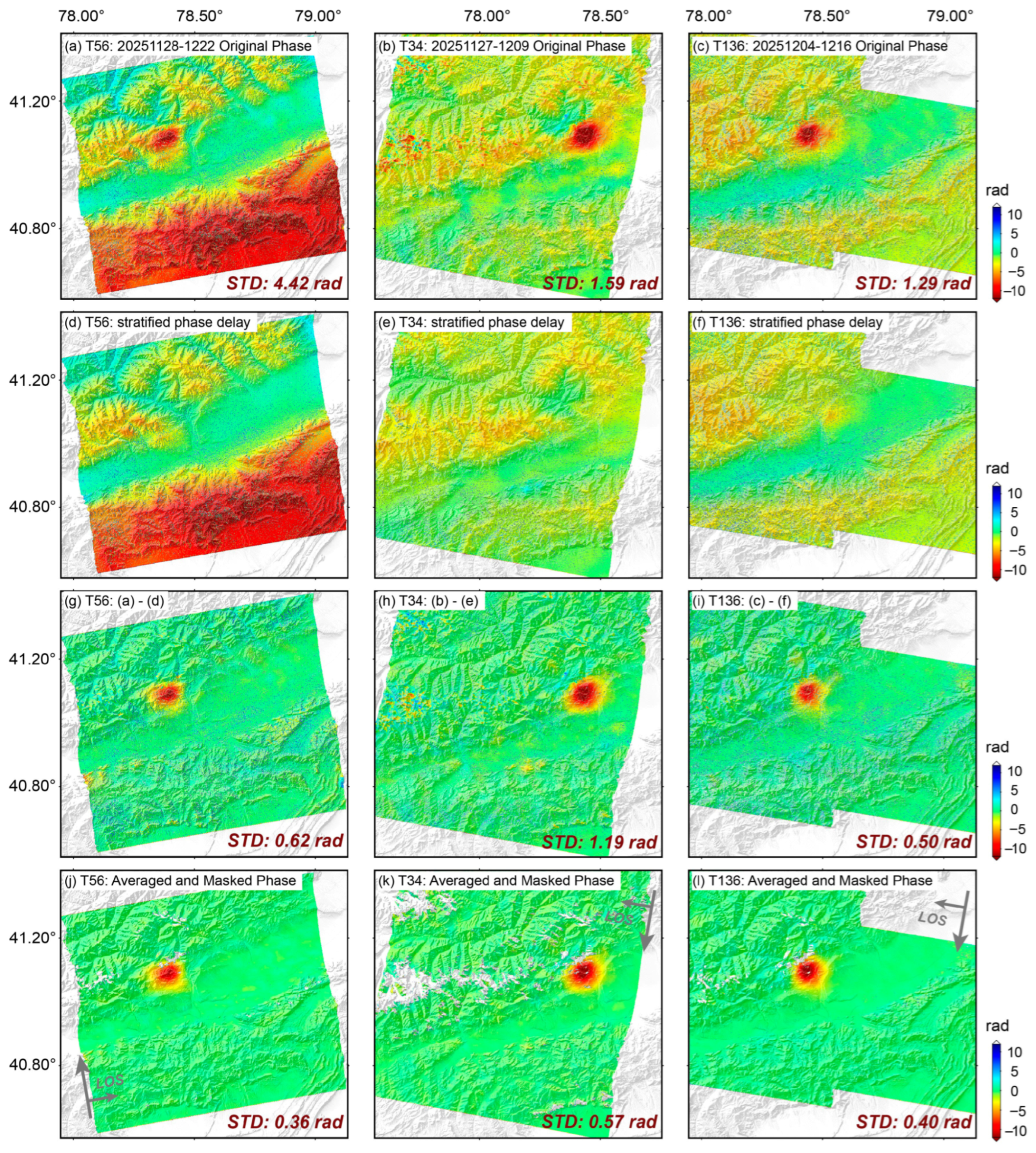
Figure 2 illustrates the tropospheric delay mitigation in InSAR coseismic deformation fields, with stratified atmospheric correction shown using one representative interferogram per track. The estimated stratified tropospheric delays effectively extract both topography-correlated phases and long-wavelength error phases. After correction, the phase standard deviations (STD) in non-deformation areas decrease from 4.42 rad, 1.59 rad, and 1.29 rad to 0.62 rad, 1.19 rad, and 0.50 rad for sample interferograms of T56, T34, and T136, respectively. Following multi-interferogram weighted averaging and low-coherence masking, these values further reduce to 0.36 rad, 0.57 rad, and 0.40 rad. Our results confirm effective tropospheric delay correction while preserving the coseismic deformation signals from the Aheqi earthquake.

3.2. Characteristics of the Coseismic Deformation Fields

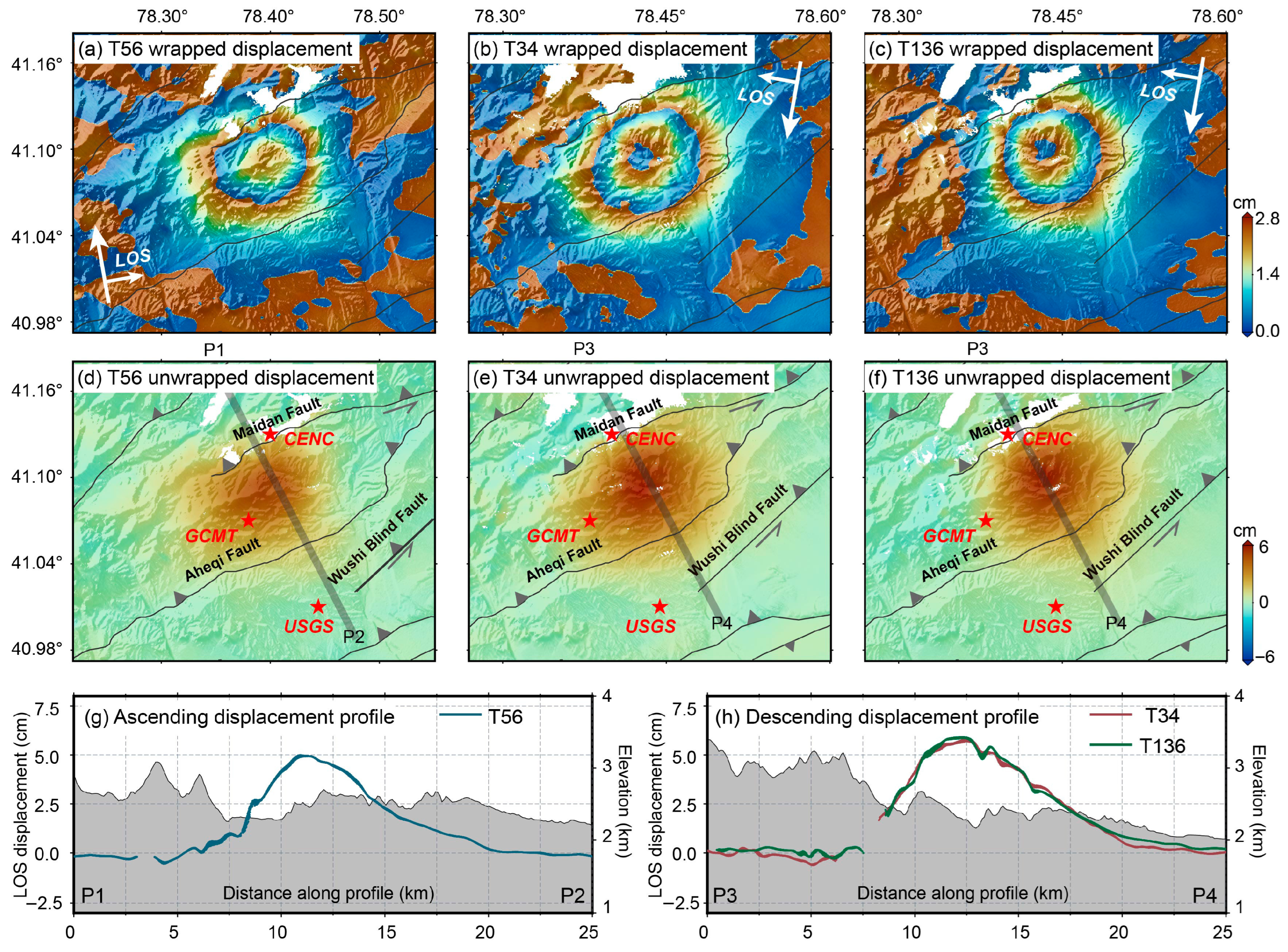
The coseismic deformation fields derived from three InSAR tracks are shown in Figure 3. Both ascending and descending tracks exhibit significant uplift, indicating the Aheqi earthquake is a thrust-faulting event. Continuous interferometric fringes suggest the rupture did not reach the surface. The maximum uplift reaches ~5.0 cm in the ascending track and ~6.0 cm in the descending track, both located between the Maidan fault and the Aheqi fault. Cross-section profiles of the deformation field show consistent gradient variations across both ascending and descending tracks (Figure 3g,h). The distance from the deformation peak to the northwestern undeformed zone (~5.0 km) is significantly shorter than to the southeastern undeformed zone (ascending: ~9.0 km; descending: ~10.0 km). The consistent asymmetry in the deformation fields suggests that a south-dipping fault plane would require a steeper dip angle than a north-dipping scenario to explain the observed displacements [46,47], which is in agreement with reported focal mechanism solutions (Table 1).

3.3. Fault Geometry from Bayesian Uniform Slip Inversion

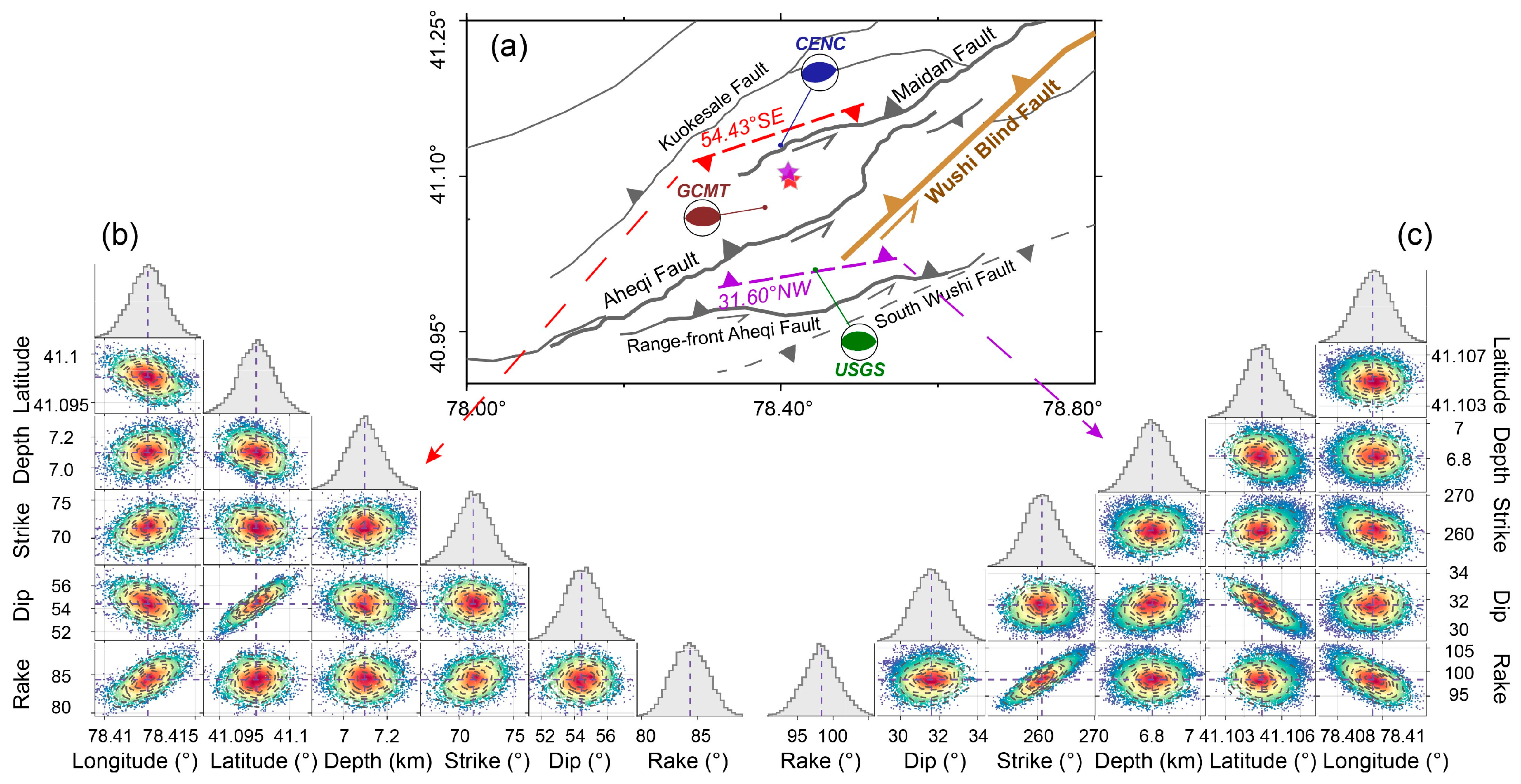
Figure 4 displays the posterior probability distributions and spatial locations of fault geometry and source parameters, all following normal distributions. The epicenter location is approximately estimated from fault geometry; thus, it shows some correlation with other parameters. When searching without strike constraints, the Bayesian algorithm identifies optimal fault parameters of 71.3 ± 1.6° (strike) and 54.4 ± 1.1° (dip), indicating a south-dipping fault. The rake angle of 84.4 ± 1.6° suggests thrust-dominated motion with a minor sinistral strike–slip component. The epicenter (78.412°E, 41.098°N) is located approximately equidistant between the Maidan fault and the Aheqi fault, showing a 3–4 km offset from the locations reported by GCMT and CENC. The hypocenter depth is 7.1 ± 0.1 km with a fault burial depth of 5.2 ± 0.2 km, indicating rupture on a blind fault. These inversion results agree well with the CENC nodal plane I parameters (72°/49°/78°) (Table 1, Figure 4b).
We subsequently impose prior north-dipping constraints in the Bayesian inversion (strike search range is set from 180° to 360°). The resolved hypocenter depth is 6.8 ± 0.1 km with a fault burial depth of 6.1 ± 0.1 km, also indicating rupture on a blind fault. The fault parameters (260.8 ± 2.1°/31.6 ± 0.9°/98.4 ± 2.5°) correspond to a north-dipping plane exhibiting primarily thrust motion with a minor dextral component. We observe a certain degree of trade-off between strike and rake angles, but we consider it to be acceptable given the small parameter uncertainties. These results show good agreement with the CENC nodal plane II parameters (270°/42°/108°; Table 1, Figure 4c).
The epicenters determined from both models show close spatial proximity (Figure 4a). We extend the fault planes along their dip directions to the surface and the fault length to 20 km. The south-dipping model exhibits strike alignment with the adjacent Maidan fault but with opposite dip direction. In contrast, the north-dipping model shows consistency in both strike and dip direction with the nearby range-front Aheqi fault, the Wushi blind fault, and the Aheqi fault. Moreover, it appears to display along-strike continuity with the Wushi blind fault. Notably, both the south-dipping and north-dipping models produce comparable root mean square errors (0.24 cm vs. 0.25 cm, respectively). Thus, the fault dip direction remains inconclusive based on current evidence.

3.4. Fault Slip Distribution and Residual Analysis

Under uniform slip assumptions, both north- and south-dipping fault models demonstrate comparable capability in explaining the InSAR data. To further evaluate these models, we perform distributed slip inversions using the Bayesian-derived geometries, comparing their kinematic patterns and residual distributions. Accounting for dip angle differences, the down-dip widths are expanded to 20 km for the north-dip fault and 16 km for the south-dip fault, respectively. The optimal smoothing factor is determined to be 0.038 through L-curve analysis that balances data misfit against model roughness (Figure S2).
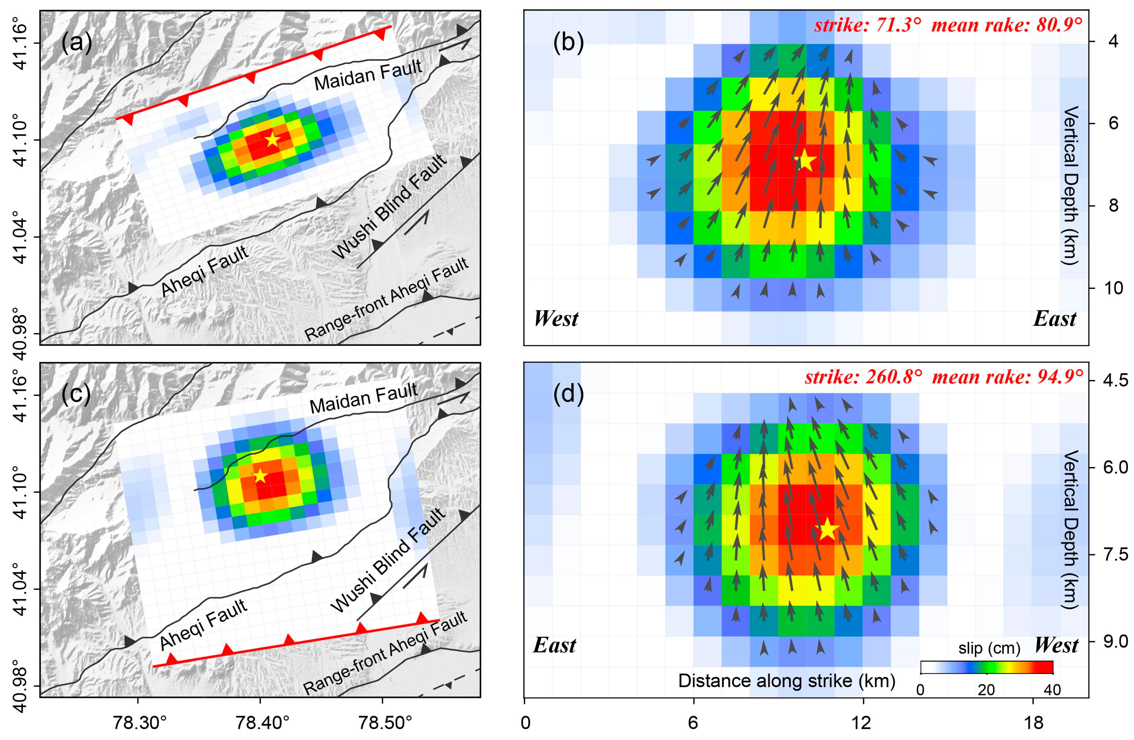
The coseismic slip distributions derived from both models are presented in Figure 5. For the south-dipping model, the inferred epicenter is located at 78.41°E, 41.10°N with a focal depth of 6.91 km (Figure 5a,b). The maximum slip amounts to ~0.38 m, with distributed slip primarily concentrated between depths of 3.5 km and 10.6 km. The slip mechanism is dominated by thrust motion (mean rake of 80.9°), accompanied by minor sinistral components near the hypocenter and dextral components in peripheral areas. Assuming a shear modulus of 30 GPa, the estimated moment magnitude is Mw 5.79. The north-dipping model determines an epicenter at 78.40°E, 41.11°N and a focal depth of 7.07 km (Figure 5c,d). The distributed slip is principally confined to depths of 4.7–9.4 km, exhibiting a peak slip of ~0.37 m. The released seismic moment corresponds to a moment magnitude of 5.81. This model similarly exhibits thrust-dominated motion (mean rake of 94.9°), but with dextral components near the hypocenter and sinistral components in some patches. Both inversion solutions consistently constrain the rupture to a blind thrust fault with a burial depth of 3–5 km. In general, the thrust-dominated patterns and calculated energy release from both models agree well with regional kinematics and reported magnitude estimates.
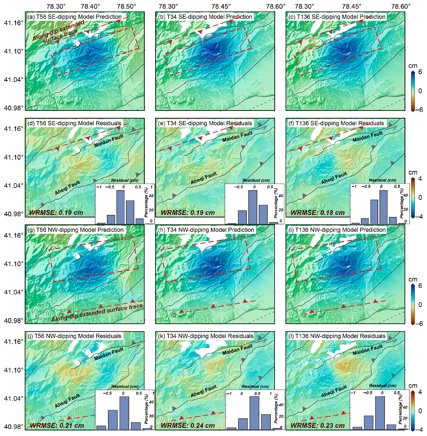
Moreover, consistent with the Bayesian uniform-slip inversion results, both dipping models in the finite-fault distributed slip inversion demonstrate comparable capability in explaining the InSAR observations. The weighted root mean square errors (WRMSE) for all three datasets are approximately 0.2 cm in both model configurations (Figure 6). Next, we further analyze the correlation between the two seismogenic models and pre-existing regional structures to identify the more plausible model.

4. Discussion

4.1. Seismogenic Fault Geometry of the Aheqi Earthquake

As a typical intracontinental reactivated orogenic belt, the South Tianshan region has developed a complex fault system under multistage tectonic evolution [1,2]. The seismogenic mechanisms of moderate-to-strong earthquakes in intracontinental orogenic belts can be broadly categorized into three models: blind thrust model, back-thrust model and shallow thrust model [48].
The blind thrust events typically occur along buried faults at the orogenic foreland or Orogen Basin boundary (e.g., Mw 7.0 Wushi earthquake). The back-thrust model includes shallow back-thrusting that occurs in thin-skinned tectonics of shallow decollements or sedimentary covers in foreland basins, and deep back-thrusting that develops above major thrust faults or in thick-skinned structures of the orogenic basement. The Mw 5.7 aftershock on 29 January 2024 represents a typical case of shallow back-thrusting. The shallow thrust events typically originate from shallow reverse faults within orogenic interiors and are often accompanied by surface rupture, such as the 2020 Mw 5.1 Sparta earthquake [49]. The Wushi mainshock and its aftershock sequence primarily involve both blind thrust and back-thrust models. Our investigation of the Mw 5.8 Aheqi earthquake reveals that its seismogenic structure corresponds to either a south-dipping back-thrust model or a north-dipping blind thrust model.
We further analyze the structural connections between these two fault models and previously investigated regional structures (Figure 7). A structural profile across the maximum coseismic slip area was constructed, extending from north to south across the Kuokesale fault, the south-dipping model, the Maidan fault, the Aheqi fault, the north-dipping model, and the range-front Aheqi fault (Figure 7). Except for the fault model of the current Aheqi earthquake, the fault dip parameters are from previous field investigations and precisely relocated earthquake catalogs [15,19].
Regarding the south-dipping back-thrust structure, our analysis reveals that although its extended surface projection locates northward of the north-dipping Maidan fault, no shallow intersection occurs as the coseismic slip is confined to depths below 3.5 km (Figure 7b). In contrast, the slip zone directly intersects the Aheqi fault, and the hypocenter is located slightly beneath it. Typically, back-thrust structures develop due to strain localization in rigid rock units within the hanging wall of major boundary faults during ongoing orogenesis, accommodating the listric geometry of the main thrust system at depth [50,51,52]. In this context, if a back-thrust structure formed as a result of strain localization in the hanging wall above the Aheqi fault, the Aheqi fault would require an exceptionally steep dip angle exceeding 75°, which is significantly greater than the dip of regional thrust faults and contradicts actual observations (30–45°) [15,20,53]. Alternatively, a major thrust fault, such as a southwestward extension of the Wushi blind fault, might exist south of the Aheqi fault. However, the limited differential uplift of the shallow strata cut by the fault, the moderate dip (50–60°) in its upper segment, and the comparable strike–slip and dip–slip components all indicate that the Wushi blind fault is an immature structure poorly aligned with the regional stress field [19], suggesting it is not stable enough to host a large back-thrust fault in its hanging wall.
Moreover, if a back-thrust fault cut across both the Aheqi fault and the range-front Aheqi fault, its coseismic rupture would likely trigger slip on one or both of these major structures or be constrained by them. In either scenario, the resulting deformation field would not appear as simple as what we observed, which is characterized by a single deformation center and regularly decaying interference fringes (Figure 3). Furthermore, the pop-up structure formed by the back-thrust and main thrust fault is typically accompanied by significant topographic relief, particularly for a significant back-thrust structure such as the proposed south-dipping model [50,54]. Nevertheless, topographic profile fails to exhibit corresponding variations that would support such a model (Figure 7b). Thus, the hypothesis of a south-dipping back-thrust fault being the seismogenic structure for the Aheqi earthquake appears highly improbable based on current evidence.
For the north-dipping model, the Bayesian-inferred fault trace extending to the surface aligns in both strike and dip with the surrounding structures, notably suggesting potential continuity with the Wushi blind thrust (Figure 4a). However, cross-sectional analysis contradicts the interpretation that the seismogenic structure is a southwestward extension of the Wushi blind thrust (Figure 7c). This is because the dip of the Wushi blind thrust is approximately twice that of our resolved seismogenic fault, and the two structures show a clear offset at depth. In contrast, although the surface traces of the Aheqi fault and the north-dipping model are offset by ~5 km, their fault planes converge at depth. Considering that the seismogenic fault of the Aheqi earthquake should exhibit a listric geometry with downward-decreasing dip angle, and given the geometric similarity between our determined fault configuration and the Aheqi fault at coseismic rupture depths, we infer that the seismogenic structure of the Mw 5.8 Aheqi earthquake is the north-dipping Aheqi fault (Figure 7c).

4.2. Stress Perturbations from the Wushi Earthquake on the Aheqi Earthquake

Major earthquakes modulate the surrounding stress field, which can promote or inhibit failure on neighboring faults [55,56,57,58]. For instance, the back-thrust aftershock on 29 January 2024 was triggered by stress loading exceeding 5 bar from the Wushi mainshock [59]. The identification of the seismogenic fault for the Aheqi earthquake enables a quantitative analysis of stress perturbations imposed by the Wushi earthquake on this event. The Coulomb failure stress change ( C F S ) is defined as [60]:
C F S = τ s + μ σ n
where τ s and σ n represent the changes in shear and normal stress on the receiver fault, respectively. μ denotes the effective friction coefficient, which is set to 0.4 following previous studies [59,61,62]. Positive C F S encourages fault rupture, while negative C F S suppresses slip. Using the published slip model of the Wushi earthquake [59] and a receiver fault constructed from the focal mechanism solution of the Aheqi earthquake as inputs, we computed the C F S on the Aheqi fault from Wushi earthquake with Coulomb 3.3 software [63].
We find that more than half of the coseismic rupture area, including the hypocenter and adjacent patches with slip exceeding 30 cm, experienced significant stress loading (Figure 8). At the hypocenter, the stress increase exceeded 2 bar, substantially surpassing the 0.1 bar earthquake triggering threshold [56,64,65], indicating a strong rupture-promoting effect from the mainshock. However, portions of the rupture zone underwent stress shadowing from the Wushi earthquake. These areas may have experienced gradual stress recovery through post-seismic afterslip-driven reloading in shallow fault sections, or pore pressure increases that reduced effective normal stress [19,58,66]. Furthermore, the rupture propagation to these areas could have been facilitated by transient dynamic Coulomb stress transfer and dynamic weakening effects induced by the preceding ruptures [67,68].

4.3. Implications for Seismic Hazards in the Southern Tianshan Orogen

Although the Aheqi and Wushi earthquakes occurred in close spatiotemporal proximity, they exhibit distinctly different fault geometries and coseismic kinematics. The Wushi earthquake involved a significant strike–slip component and ruptured through the basement along a high-angle inherited plane of weakness that is not optimally oriented with the prevailing stress field [19]. In contrast, the Aheqi earthquake was dominated by thrust motion, with rupture terminating at the decollement, which is consistent with both the structural geometry of the widespread fold-and-thrust belts in the southern Tianshan and the regional background stress field. As shown in Figure 7, the Maidan fault, together with the Aheqi fault, constitutes a major Orogen Basin boundary structure along the southern Tianshan piedmont. Toward the mountain interior from the Aheqi fault, the structures consistently cut through the sedimentary cover and the regional decollement, with their penetration into the basement becoming progressively deeper. This transition to deep basement-involved faulting accommodates large-scale crustal shortening, which is expressed in the regional topography as a pronounced uplift of ~2 km between the Aheqi and the Kuokesale faults (Figure 7). These boundary structures were reactivated in the Cenozoic due to far-field effects of the India-Eurasia collision and has since evolved into its current prominent form through continued plate convergence [1,2,69]. The significant stress loading from the Wushi earthquake on the Aheqi earthquake suggests that the reactivation of ancient structures, i.e., the Wushi blind fault, may advance rupture on currently active faults. This highlights the necessity of incorporating pre-existing planes of weakness into seismic hazard assessments.
The Aheqi earthquake exhibits a magnitude comparable to those of events occurring along the Kepingtage FTB in recent decades. These events are typically characterized by continuous surface deformation with no observable surface rupture [11,70]. On one hand, most earthquakes in this belt occur within the sedimentary cover, which, due to its limited capacity for elastic strain accumulation compared to the underlying basement, tends to release strain energy through frequent moderate events [11]. On the other hand, the causative faults are thrust faults exhibiting variable dip angles, displaying a listric geometry with steep upper segments and gentler lower segments [8,21]. Ruptures nucleating at depth are hindered from propagating upward to the surface due to the fault bending, instead producing shallow folding within the hanging-wall cover [22,71]. This structural barrier likewise limits the maximum possible earthquake magnitude.

4.4. Capability of InSAR Technique in Resolving Fault Geometry and Slip for Moderate Blind Thrust Earthquakes

In constraining the seismogenic fault of the Aheqi earthquake using InSAR, both Bayesian uniform-slip and finite-fault distributed-slip inversions produced similarly small residuals for the north- and south-dipping models. This highlights the ambiguity in extracting fault geometry for moderate-magnitude blind thrust earthquakes using InSAR observations, as observed in previous studies [26,47,54]. Notably, the optimal dip direction obtained from an unconstrained Bayesian inversion (south-dipping) opposes our preferred north-dipping solution, underscoring the importance of evaluating both candidate dip models for blind thrust events.
Consequently, additional constraints from regional tectonics are required to distinguish between competing models. Different structures develop under specific conditions and produce distinct geomorphic signatures. For instance, a back-thrust requires long-term strain localization within the hanging wall of a major thrust fault and generates pronounced uplift. In contrast, blind thrust faults are typically characterized by the growth of an anticline above its propagating tip. Furthermore, the geometric relationship between the seismogenic model and the existing structures also serves as a check against the observed surface deformation. For instance, a simple and regular InSAR deformation field suggests a correspondingly simple fault geometry at depth, and should not result from a complex, intersecting fault system.
Moreover, in thrust-dominated moderate-magnitude earthquakes, the horizontal displacement signals in the deformation field are typically too weak, making it potentially difficult to accurately constrain the direction of strike–slip component. Our inversion results for both models show mixed sinistral and dextral slip distributions. More refined slip distribution could be obtained through time-series InSAR methods, though this would require sufficient post-seismic data accumulation [72].

5. Conclusions

In this study, we investigated the coseismic surface deformation and seismogenic structure of the 4 December 2025, Mw 5.8 Aheqi, Xinjiang earthquake using InSAR data and dislocation modeling. A moving-window linear model and a multi-interferogram weighted averaging strategy were employed to mitigate elevation-correlated tropospheric delay and turbulent atmospheric noise in the deformation fields. The derived deformation fields are dominated by uplift, with maximum displacements of ~5.0 cm and ~6.0 cm for the ascending and descending tracks, respectively, indicating a thrust-dominated mechanism.
Bayesian uniform slip inversion revealed two possible mechanisms: a back-thrust, characterized by a south-dipping (54.4°, strike 71.3°) blind fault, and a blind thrust, characterized by a north-dipping (31.6°, strike 260.8°) fault. Both models satisfactorily explained the InSAR data in distributed slip inversions. Further analysis suggests a low probability for the south-dipping back-thrust model, given its inconsistency with pre-existing structures, the coseismic deformation pattern, and the lack of supportive topographic expression. Conversely, the blind thrust model is supported by the deep geometry of the pre-existing Aheqi fault, which we consequently identified as the seismogenic structure.
The ruptured Aheqi fault is situated in the hinterland of the southern Tianshan thrust belt and, together with the steeper Maidan fault to the north, constitutes a major Orogen Basin boundary. Coulomb stress change calculations indicate significant stress loading (>2 bar) from the Wushi earthquake onto the hypocenter of the Aheqi earthquake, suggesting a rupture-advancing relationship. This suggests that earthquakes on reactivated structures may promote failure on present-day active faults, indicating a potential for sequential rupture from inherited planes of weakness. Consequently, such cascading potential should be considered in future seismic hazard frameworks for the southern Tianshan orogen.

Supplementary Materials

The following supporting information can be downloaded at: https://www.mdpi.com/article/10.3390/rs18071078/s1, Figure S1: Convergence of MCMC samples; Figure S2: Determination of the smoothing factor used in slip distribution inversion; Table S1: Weights assigned to interferograms based on variogram fitting.

Author Contributions

Conceptualization, K.S. and L.X.; methodology, K.S.; software, K.S., N.F. and P.Z.; formal analysis, K.S., N.F. and Z.C.; writing—original draft preparation, K.S. and Z.C.; writing—review and editing, L.X.; visualization, K.S.; funding acquisition, L.X. and K.S. All authors have read and agreed to the published version of the manuscript.

Funding

This research was funded by the National Natural Science Foundation of China (42304037), the Natural Science Foundation of Hunan Province (2025JJ60239, 2024JJ3031), the Science and Technology Innovation Program of Fujian Province (2021Y3001), the Science and Technology Innovation Program of Hunan Province (2023SK2012), the State grid corporation of China headquarters science and technology project (52199925001N-225-TD), the Fundamental Research Funds for the Central Universities of Central South University (2024ZZTS0368), and the Earthquake Prevention and Disaster Reduction Research Project of Hunan Earthquake Agency (202503).

Data Availability Statement

Sentinel-1 and Sentinel-2 data are available for download via the Copernicus Data Space Ecosystem at https://browser.dataspace.copernicus.eu/ (accessed on 25 February 2026). The GBIS (Geodetic Bayesian Inversion Software v1.1) can be accessed at https://comet.nerc.ac.uk/geodetic-Bayesian-inversion-software-gbis/ (accessed on 25 February 2026). Coulomb 3.3 software is available at https://temblor.net/coulomb/ (accessed on 25 February 2026). The raw data supporting the conclusions of this article will be made available by the authors on request.

Acknowledgments

We thank the four anonymous reviewers for their constructive comments. We thank Ping He for insightful discussions on the fault dip determination. All figures are produced by Generic Mapping Tools 6.4.0 software [73].

Conflicts of Interest

The authors declare no conflicts of interest.

References

  1. Tapponnier, P.; Molnar, P. Active Faulting and Cenozoic Tectonics of the Tien Shan, Mongolia, and Baykal Regions. J. Geophys. Res. Solid Earth 1979, 84, 3425–3459. [Google Scholar] [CrossRef] [Scilit]
  2. Yin, A.; Nie, S.; Craig, P.; Harrison, T.M.; Ryerson, F.J.; Qian, X.; Geng, Y. Late Cenozoic Tectonic Evolution of the Southern Chinese Tian Shan. Tectonics 1998, 17, 1–27. [Google Scholar] [CrossRef] [Scilit]
  3. Tapponnier, P.; Xu, Z.; Roger, F.; Meyer, B.; Arnaud, N.; Wittlinger, G.; Yang, J. Oblique Stepwise Rise and Growth of the Tibet Plateau. Science 2001, 294, 1671–1677. [Google Scholar] [CrossRef] [Scilit]
  4. Abdrakhmatov, K.Y.; Aldazhanov, S.A.; Hager, B.H.; Hamburger, M.W.; Herring, T.A.; Kalabaev, K.B.; Makarov, V.I.; Molnar, P.; Panasyuk, S.V.; Prilepin, M.T.; et al. Relatively Recent Construction of the Tien Shan Inferred from GPS Measurements of Present-Day Crustal Deformation Rates. Nature 1996, 384, 450–453. [Google Scholar] [CrossRef] [Scilit]
  5. Reigber, C.; Michel, G.W.; Galas, R.; Angermann, D.; Klotz, J.; Chen, J.Y.; Papschev, A.; Arslanov, R.; Tzurkov, V.E.; Ishanov, M.C. New Space Geodetic Constraints on the Distribution of Deformation in Central Asia. Earth Planet. Sci. Lett. 2001, 191, 157–165. [Google Scholar] [CrossRef] [Scilit]
  6. Zubovich, A.V.; Wang, X.; Scherba, Y.G.; Schelochkov, G.G.; Reilinger, R.; Reigber, C.; Mosienko, O.I.; Molnar, P.; Michajljow, W.; Makarov, V.I.; et al. GPS Velocity Field for the Tien Shan and Surrounding Regions. Tectonics 2010, 29, TC6014. [Google Scholar] [CrossRef] [Scilit]
  7. Wu, C.; Zhang, P.; Zhang, Z.; Zheng, W.; Xu, B.; Wang, W.; Yu, Z.; Dai, X.; Zhang, B.; Zang, K. Slip Partitioning and Crustal Deformation Patterns in the Tianshan Orogenic Belt Derived from GPS Measurements and Their Tectonic Implications. Earth-Sci. Rev. 2023, 238, 104362. [Google Scholar] [CrossRef] [Scilit]
  8. Yang, S.; Li, J.; Wang, Q. The Deformation Pattern and Fault Rate in the Tianshan Mountains Inferred from GPS Observations. Sci. China Ser. Earth Sci. 2008, 51, 1064–1080. [Google Scholar] [CrossRef] [Scilit]
  9. Lu, H.; Li, B.; Wu, D.; Zhao, J.; Zheng, X.; Xiong, J.; Li, Y. Spatiotemporal Patterns of the Late Quaternary Deformation across the Northern Chinese Tian Shan Foreland. Earth-Sci. Rev. 2019, 194, 19–37. [Google Scholar] [CrossRef] [Scilit]
  10. Wang, M.; Shen, Z.-K. Present-Day Crustal Deformation of Continental China Derived From GPS and Its Tectonic Implications. J. Geophys. Res. Solid Earth 2020, 125, e2019JB018774. [Google Scholar] [CrossRef] [Scilit]
  11. Chen, Z.; Fang, N.; Xu, W.; Yao, Y.; Zhou, P.; Xie, L.; Zhao, L. Folding Growth Pattern of the Southern Tian Shan: Insights from the 2024 Mw 7.0 Wushi Earthquake and 2020 Mw 6.0 Jiashi Earthquake, Western China. Seismol. Res. Lett. 2025, 97, 637–650. [Google Scholar] [CrossRef] [Scilit]
  12. He, P.; Wen, Y.; Wang, X.; Hooper, A.; Xu, G. Coseismic, Aftershock, and Early Postseismic Deformation During the 2024 Mw 7.0 Wushi Earthquake Sequence, Xinjiang Province, China. J. Geophys. Res. Solid Earth 2025, 130, e2024JB030364. [Google Scholar] [CrossRef] [Scilit]
  13. Ma, C.; Wei, Z.; Qian, L.; Li, T.; Li, C.; Xi, X.; Deng, Y.; Geng, S. Study of the Characteristics of a Co-Seismic Displacement Field Based on High-Resolution Stereo Imagery: A Case Study of the 2024 MS7.1 Wushi Earthquake, Xinjiang. Remote Sens. 2025, 17, 2625. [Google Scholar] [CrossRef] [Scilit]
  14. Qiu, J.; Sun, J.; Ji, L. The 2024 Mw 7.1 Wushi Earthquake: A Thrust and Strike-Slip Event Unveiling the Seismic Mechanisms of the South Tian Shan’s Thick-Skin Tectonics. Remote Sens. 2024, 16, 2937. [Google Scholar] [CrossRef] [Scilit]
  15. Wang, S.; Fang, L.; Chevalier, M.-L.; Li, H.; Li, J.; Huang, L.; Pan, J.; Ran, H.; Liang, P.; Fan, L.; et al. Seismogenic Fault Model of the 2024 Mw 7.0 Wushi Earthquake, Western China, from Geomorphology and Aftershock Relocation. GSA Bull. 2025. [Google Scholar] [CrossRef] [Scilit]
  16. Li, H.; Pan, J.; Chevalier, M.-L.; Liu, D.; Wang, S.; Luo, H.; Zhang, L.; Fang, L.; Wang, T.; Liu, F.; et al. Aftershock-Induced Surface Ruptures Overshadow the 2024 Mw 7.0 Wushi Mainshock, China. Geology 2025, 54, 105–110. [Google Scholar] [CrossRef] [Scilit]
  17. Zhang, B.X.; Qian, L.; Li, T.; Chen, J.; Xu, J.H.; Yao, Y.; Fang, L.H.; Xie, C.; Chen, J.B.; Liu, G.S.; et al. Geological Disasters and Surface Ruptures of January 23, 2024 Ms 7.1 Wushi Earthquake, Xinjiang, China. Seismol. Geol. Chin. 2024, 46, 220–234. [Google Scholar]
  18. Thompson Jobe, J.A.; Hanagan, C.E.; Hatem, A.E.; Barnhart, W.D.; Goldberg, D.E.; Yeck, W.L. Surface Rupture from an Aftershock: Remote Observations from the January 2024 Wushi (Aykol), China, Earthquakes. Seismol. Res. Lett. 2025, 96, 3490–3510. [Google Scholar] [CrossRef]
  19. Yin, X.; Li, T.; Zhang, Y.; Peng, Z.; Dal Zilio, L.; Chen, Z.; Cui, H.; Qian, L.; Sun, X.; Lu, R.; et al. Interlacing Ruptures of the 2024 Wushi Earthquake (Chinese Tian Shan) Controlled by Structural Inheritance. Commun. Earth Environ. 2025, 6, 908. [Google Scholar] [CrossRef] [Scilit]
  20. Turner, S.A.; Cosgrove, J.W.; Liu, J.G. Controls on Lateral Structural Variability along the Keping Shan Thrust Belt, SW Tien Shan Foreland, China. Geol. Soc. Lond. Spec. Publ. 2010, 348, 71–85. [Google Scholar] [CrossRef] [Scilit]
  21. Yao, Y.; Wen, S.; Li, T.; Wang, C. The 2020 Mw 6.0 Jiashi Earthquake: A Fold Earthquake Event in the Southern Tian Shan, Northwest China. Seismol. Res. Lett. 2020, 92, 859–869. [Google Scholar] [CrossRef] [Scilit]
  22. Lü, L.; Sun, J.; Jia, Y.; Wu, L. Late Cenozoic Thrust Propagation within the Keping Fold-and-Thrust Belt along the Southern Foreland of Chinese Tian Shan: Evidence from Apatite (UTh)/He Results. Tectonophysics 2021, 814, 228966. [Google Scholar] [CrossRef] [Scilit]
  23. Cakir, Z.; Meghraoui, M.; Akoglu, A.M.; Jabour, N.; Belabbes, S.; Ait-Brahim, L. Surface Deformation Associated with the Mw 6.4, 24 February 2004 Al Hoceima, Morocco, Earthquake Deduced from InSAR: Implications for the Active Tectonics along North Africa. Bull. Seismol. Soc. Am. 2006, 96, 59–68. [Google Scholar] [CrossRef] [Scilit]
  24. He, P.; Wang, Q.; Ding, K.; Wang, M.; Qiao, X.; Li, J.; Wen, Y.; Xu, C.; Yang, S.; Zou, R. Source Model of the 2015 Mw 6.4 Pishan Earthquake Constrained by Interferometric Synthetic Aperture Radar and GPS: Insight into Blind Rupture in the Western Kunlun Shan. Geophys. Res. Lett. 2016, 43, 1511–1519. [Google Scholar] [CrossRef] [Scilit]
  25. Chen, K.; Xu, W.; Mai, P.M.; Gao, H.; Zhang, L.; Ding, X. The 2017 Mw 7.3 Sarpol Zahāb Earthquake, Iran: A Compact Blind Shallow-Dipping Thrust Event in the Mountain Front Fault Basement. Tectonophysics 2018, 747–748, 108–114. [Google Scholar] [CrossRef] [Scilit]
  26. Huang, X.; Li, Y.; Shan, X.; Zhong, M.; Wang, X.; Gao, Z. Fault Kinematics of the 2023 Mw 6.0 Jishishan Earthquake, China, Characterized by Interferometric Synthetic Aperture Radar Observations. Remote Sens. 2024, 16, 1746. [Google Scholar] [CrossRef] [Scilit]
  27. Fang, N.; Chen, Z.; Zhao, L.; Sun, K.; Xie, L.; Xu, W. Joint Inversion of InSAR and Seismic Data Unveiling the Dynamic Rupture Process and Seismotectonic Kinematics of the 2023 Mw 6.8 Morocco Earthquake. Remote Sens. 2025, 17, 2971. [Google Scholar] [CrossRef] [Scilit]
  28. Feng, W.; Li, Z. A Novel Hybrid PSO/Simplex Algorithm for Determining Earthquake Source Parameters Using InSAR Data. Prog. Geophys. 2010, 25, 1189–1196. [Google Scholar] [CrossRef]
  29. Amighpey, M.; Voosoghi, B.; Motagh, M. Deformation and Fault Parameters of the 2005 Qeshm Earthquake in Iran Revisited: A Bayesian Simulated Annealing Approach Applied to the Inversion of Space Geodetic Data. Int. J. Appl. Earth Obs. Geoinf. 2014, 26, 184–192. [Google Scholar] [CrossRef] [Scilit]
  30. Bagnardi, M.; Hooper, A. Inversion of Surface Deformation Data for Rapid Estimates of Source Parameters and Uncertainties: A Bayesian Approach. Geochem. Geophys. Geosyst. 2018, 19, 2194–2211. [Google Scholar] [CrossRef] [Scilit]
  31. Wei, G.; Chen, K.; Meng, H. Bayesian Inversion of Finite-Fault Earthquake Slip Model Using Geodetic Data, Solving for Non-Planar Fault Geometry, Variable Slip, and Data Weighting. J. Geophys. Res. Solid Earth 2023, 128, e2022JB025225. [Google Scholar] [CrossRef] [Scilit]
  32. Chang, F.; Fang, J.; Dong, S.; Yin, H.; Rollins, C.; Elliott, J.R.; Hooper, A.J. Geodetic Strain Rates, Slip Deficit Rates, and Seismic Potential in the Tianshan, Central Asia. Geophys. Res. Lett. 2025, 52, e2025GL118470. [Google Scholar] [CrossRef] [Scilit]
  33. Wegnüller, U.; Werner, C.; Strozzi, T.; Wiesmann, A.; Frey, O.; Santoro, M. Sentinel-1 Support in the GAMMA Software. Procedia Comput. Sci. 2016, 100, 1305–1312. [Google Scholar] [CrossRef] [Scilit]
  34. Farr, T.G.; Rosen, P.A.; Caro, E.; Crippen, R.; Duren, R.; Hensley, S.; Kobrick, M.; Paller, M.; Rodriguez, E.; Roth, L.; et al. The Shuttle Radar Topography Mission. Rev. Geophys. 2007, 45, RG2004. [Google Scholar] [CrossRef] [Scilit]
  35. Goldstein, R.M.; Werner, C.L. Radar Interferogram Filtering for Geophysical Applications. Geophys. Res. Lett. 1998, 25, 4035–4038. [Google Scholar] [CrossRef] [Scilit]
  36. Costantini, M. A Novel Phase Unwrapping Method Based on Network Programming. IEEE Trans. Geosci. Remote Sens. 1998, 36, 813–821. [Google Scholar] [CrossRef] [Scilit]
  37. Chen, C.W.; Zebker, H.A. Phase Unwrapping for Large SAR Interferograms: Statistical Segmentation and Generalized Network Models. IEEE Trans. Geosci. Remote Sens. 2002, 40, 1709–1719. [Google Scholar] [CrossRef] [Scilit]
  38. Sha, P.; He, X.; Wang, X.; Gao, Z. Large-Scale Crustal Deformation of the Tianshan Mountains, Xinjiang, from Sentinel-1 InSAR Observations (2015–2020). Remote Sens. 2023, 15, 4901. [Google Scholar] [CrossRef] [Scilit]
  39. Gong, W.; Zhao, D.; Zhu, C.; Zhang, Y.; Li, C.; Zhang, G.; Shan, X. A New Method for InSAR Stratified Tropospheric Delay Correction Facilitating Refinement of Coseismic Displacement Fields of Small-to-Moderate Earthquakes. Remote Sens. 2022, 14, 1425. [Google Scholar] [CrossRef] [Scilit]
  40. Wang, Y.; Dong, J.; Zhang, L.; Zhang, L.; Deng, S.; Zhang, G.; Liao, M.; Gong, J. Refined InSAR Tropospheric Delay Correction for Wide-Area Landslide Identification and Monitoring. Remote Sens. Environ. 2022, 275, 113013. [Google Scholar] [CrossRef] [Scilit]
  41. Cavalié, O.; Doin, M.-P.; Lasserre, C.; Briole, P. Ground Motion Measurement in the Lake Mead Area, Nevada, by Differential Synthetic Aperture Radar Interferometry Time Series Analysis: Probing the Lithosphere Rheological Structure. J. Geophys. Res. Solid Earth 2007, 112, B03403. [Google Scholar] [CrossRef] [Scilit]
  42. Fattahi, H.; Amelung, F. InSAR Bias and Uncertainty Due to the Systematic and Stochastic Tropospheric Delay. J. Geophys. Res. Solid Earth 2015, 120, 8758–8773. [Google Scholar] [CrossRef] [Scilit]
  43. Okada, Y. Surface Deformation Due to Shear and Tensile Faults in a Half-Space. Bull. Seismol. Soc. Am. 1985, 75, 1135–1154. [Google Scholar] [CrossRef] [Scilit]
  44. Jónsson, S.; Zebker, H.; Segall, P.; Amelung, F. Fault Slip Distribution of the 1999 Mw 7.1 Hector Mine, California, Earthquake, Estimated from Satellite Radar and GPS Measurements. Bull. Seismol. Soc. Am. 2002, 92, 1377–1389. [Google Scholar] [CrossRef] [Scilit]
  45. Wang, R.; Parolai, S.; Ge, M.; Jin, M.; Walter, T.R.; Zschau, J. The 2011 Mw 9.0 Tohoku Earthquake: Comparison of GPS and Strong-Motion Data. Bull. Seismol. Soc. Am. 2013, 103, 1336–1347. [Google Scholar] [CrossRef] [Scilit]
  46. Sethanant, I.; Nissen, E. The InSAR Lookbook: An Illustrated Guide to Earthquake Deformation Interferograms. Seismica 2025, 4, 1–39. [Google Scholar] [CrossRef] [Scilit]
  47. Zhang, Y.; Shan, X.; Gong, W.; Zhang, G. The Ambiguous Fault Geometry Derived from InSAR Measurements of Buried Thrust Earthquakes: A Synthetic Data Based Study. Geophys. J. Int. 2021, 225, 1799–1811. [Google Scholar] [CrossRef] [Scilit]
  48. Guo, P.; Han, Z.; Zhou, C.; Gai, H.; Niu, P.; Zhang, X. Multi-Segment Ruptures of the 2023 Mw 6.0 Jishishan Earthquake, Tibetan Plateau: Implications for Seismogenic Mechanisms of Moderate Earthquakes. J. Geophys. Res. Solid Earth 2025, 130, e2024JB029368. [Google Scholar] [CrossRef] [Scilit]
  49. Figueiredo, P.; Hill, J.; Merschat, A.; Scheip, C.; Stewart, K.; Owen, L.; Wooten, R.; Carter, M.; Szymanski, E.; Horton, S.; et al. The Mw 5.1, 9 August 2020, Sparta Earthquake, North Carolina: The First Documented Seismic Surface Rupture in the Eastern United States. GSA Today 2022, 32, 4–11. [Google Scholar] [CrossRef] [Scilit]
  50. Morley, C.K. A Classification of Thrust Fronts. AAPG Bull. 1986, 70, 12–25. [Google Scholar] [CrossRef] [Scilit]
  51. Butler, R.W.H. Thrust Sequences. J. Geol. Soc. 1987, 144, 619–634. [Google Scholar] [CrossRef] [Scilit]
  52. Erslev, E.A. Thrusts, Back-Thrusts, and Detachment of Rocky Mountain Foreland Arches. In Laramide Basement Deformation in the Rocky Mountain Foreland of the Western United States; Schmidt, C.J., Chase, R.B., Erslev, E.A., Eds.; Geological Society of America: Boulder, CO, USA, 1993; pp. 339–358. ISBN 978-0-8137-2280-1. [Google Scholar]
  53. Wu, C.; Zheng, W.; Zhang, P.; Zhang, Z.; Jia, Q.; Yu, J.; Zhang, H.; Yao, Y.; Liu, J.; Han, G.; et al. Oblique Thrust of the Maidan Fault and Late Quaternary Tectonic Deformation in the Southwestern Tian Shan, Northwestern China. Tectonics 2019, 38, 2625–2645. [Google Scholar] [CrossRef] [Scilit]
  54. He, P.; Hetland, E.A.; Niemi, N.A.; Wang, Q.; Wen, Y.; Ding, K. The 2016 Mw 6.5 Nura Earthquake in the Trans Alai Range, Northern Pamir: Possible Rupture on a Back-Thrust Fault Constrained by Sentinel-1A Radar Interferometry. Tectonophysics 2018, 749, 62–71. [Google Scholar] [CrossRef] [Scilit]
  55. Stein, R.S.; King, G.C.P.; Lin, J. Change in Failure Stress on the Southern San Andreas Fault System Caused by the 1992 Magnitude = 7.4 Landers Earthquake. Science 1992, 258, 1328–1332. [Google Scholar] [CrossRef] [Scilit] [PubMed]
  56. King, G.C.P.; Stein, R.S.; Lin, J. Static Stress Changes and the Triggering of Earthquakes. Bull. Seismol. Soc. Am. 1994, 84, 935–953. [Google Scholar] [CrossRef] [Scilit]
  57. Toda, S.; Lin, J.; Meghraoui, M.; Stein, R.S. 12 May 2008 M = 7.9 Wenchuan, China, Earthquake Calculated to Increase Failure Stress and Seismicity Rate on Three Major Fault Systems. Geophys. Res. Lett. 2008, 35, L17305. [Google Scholar] [CrossRef] [Scilit]
  58. Liu, X.; Xu, W.; Frank, W.B.; Zhou, Y.; Zhao, G.; Fang, L.; Huang, H.; He, L.; Gan, W. Rheological and Tectonic Implications of Eastern Tibet: Insights from Early Aftershock Sequences Driven by Afterslip Following Three 2021–2022 Moderate-Large Events. Int. J. Appl. Earth Obs. Geoinf. 2025, 143, 104770. [Google Scholar] [CrossRef] [Scilit]
  59. Zhou, P.; Xu, W.B.; Bai, C.Y.; Chen, Z.D.; Huang, C.C.; Xie, L.; Li, Z.Y. Inversion of the Listric Fault Structure and Early Postseismic Slip Distribution of the 2024 Xinjiang Wushi Mw7.0 Earthquake Based on InSAR Data. Chin. J. Geophys. Chin. 2025, 68, 4181–4193. [Google Scholar] [CrossRef]
  60. Harris, R.A. Introduction to Special Section: Stress Triggers, Stress Shadows, and Implications for Seismic Hazard. J. Geophys. Res. Solid Earth 1998, 103, 24347–24358. [Google Scholar] [CrossRef] [Scilit]
  61. Freed, A.M. Earthquake Triggering by Static, Dynamic, and Postseismic Stress Transfer. Annu. Rev. Earth Planet. Sci. 2005, 33, 335–367. [Google Scholar] [CrossRef] [Scilit]
  62. Famiglietti, N.A.; Cheloni, D.; Caputo, R.; Vicari, A. Geodetic Model of the 2024 January 22 Mw 7.0 Wushi (Northwestern China) Earthquake and Mw 5.7 Aftershock from Inversion of InSAR Data. Geophys. J. Int. 2025, 241, 941–953. [Google Scholar] [CrossRef] [Scilit]
  63. Toda, S.; Stein, R.S.; Sevilgen, V.; Lin, J. Coulomb 3.3 Graphic-Rich Deformation and Stress-Change Software for Earthquake, Tectonic, and Volcano Research and Teaching—User Guide. US Geol. Surv. Open-File Rep. 2011, 1060, 63. [Google Scholar]
  64. Reasenberg, P.A.; Simpson, R.W. Response of Regional Seismicity to the Static Stress Change Produced by the Loma Prieta Earthquake. Science 1992, 255, 1687–1690. [Google Scholar] [CrossRef] [Scilit]
  65. Stein, R.S. The Role of Stress Transfer in Earthquake Occurrence. Nature 1999, 402, 605–609. [Google Scholar] [CrossRef] [Scilit]
  66. Liu, X.; Xie, L.; Zheng, A.; Zheng, Y.; Gunatilake, T.; Yang, J.; He, L.; Ganas, A. The Role of Post-Earthquake Fluid Pressure in Driving the 2021 Thessaly (Greece) Aftershock Sequence. J. Earth Sci. 2025, 36, 2836–2841. [Google Scholar] [CrossRef] [Scilit]
  67. Kilb, D.; Gomberg, J.; Bodin, P. Triggering of Earthquake Aftershocks by Dynamic Stresses. Nature 2000, 408, 570–574. [Google Scholar] [CrossRef] [Scilit]
  68. Jia, Z.; Jin, Z.; Marchandon, M.; Ulrich, T.; Gabriel, A.-A.; Fan, W.; Shearer, P.; Zou, X.; Rekoske, J.; Bulut, F.; et al. The Complex Dynamics of the 2023 Kahramanmaraş, Turkey, Mw 7.8–7.7 Earthquake Doublet. Science 2023, 381, 985–990. [Google Scholar] [CrossRef] [Scilit] [PubMed]
  69. Xiao, W.; Song, D.; Windley, B.F.; Li, J.; Han, C.; Wan, B.; Zhang, J.; Ao, S.; Zhang, Z. Accretionary Processes and Metallogenesis of the Central Asian Orogenic Belt: Advances and Perspectives. Sci. China Earth Sci. 2020, 63, 329–361. [Google Scholar] [CrossRef] [Scilit]
  70. Lü, L.; Li, T.; Chen, Z.; Chen, J.; Jobe, J.T.; Fang, L. Active Structural Geometries and Their Correlation With Moderate (M 5.5–7.0) Earthquakes in the Jiashi-Keping Region, Tian Shan Southwestern Front. Tectonics 2021, 40, e2021TC006760. [Google Scholar] [CrossRef] [Scilit]
  71. Suppe, J. Geometry and Kinematics of Fault-Bend Folding. Am. J. Sci. 1983, 283, 684–721. [Google Scholar] [CrossRef] [Scilit]
  72. Liu, F.; Elliott, J.R.; Craig, T.J.; Hooper, A.; Wright, T.J. Improving the Resolving Power of InSAR for Earthquakes Using Time Series: A Case Study in Iran. Geophys. Res. Lett. 2021, 48, e2021GL093043. [Google Scholar] [CrossRef] [Scilit]
  73. Wessel, P.; Luis, J.F.; Uieda, L.; Scharroo, R.; Wobbe, F.; Smith, W.H.F.; Tian, D. The Generic Mapping Tools Version 6. Geochem. Geophys. Geosyst. 2019, 20, 5556–5564. [Google Scholar] [CrossRef] [Scilit]
Figure 2. Tropospheric Delay Mitigation for InSAR coseismic deformation fields. (ac) Original unwrapped phase of T56 (20251128–20251222), T34 (20251127–20251209), and T136 (20251204–20251216). (df) Extracted stratified tropospheric phase. (gi) Phase after removing stratified tropospheric delays. (jl) Final phase after weighted averaging of four interferometric pairs with masking of low-coherence areas (coherence ≤ 0.85) and snow-covered regions. Negative values indicate motion toward the satellite.
Remotesensing 18 01078 g002
Figure 3. Coseismic deformation fields and surface deformation profiles of the Aheqi earthquake. (ac) Interferometric fringe patterns for tracks T56, T34, and T136; (df) Unwrapped deformation fields corresponding to T56, T34, and T136. The red stars show the epicenter locations of the Aheqi earthquake from different institutions. (g,h) Deformation profiles along the ascending (P1–P2) and descending (P3–P4) tracks, respectively. Positive values indicate uplift deformation. Line width reflects the data density.
Remotesensing 18 01078 g003
Figure 4. Fault geometry of the Aheqi earthquake from Bayesian uniform-slip inversion. (a) Comparison of south- and south-dipping model solutions with adjacent fault properties. (b) hypocenter location and fault parameters for the south-dipping model. (c) Hypocenter location and fault parameters for the north-dipping model.
Remotesensing 18 01078 g004
Figure 5. Coseismic slip distribution of the Aheqi earthquake. (a,b): South-dipping model; (c,d): North-dipping model. The yellow star denotes the inverted hypocenter location. The arrows indicate the slip directions of fault patches.
Remotesensing 18 01078 g005
Figure 6. Model predictions and residuals. (ac) Predicted displacements from the south-dipping model for T56, T34, and T136 tracks, respectively; (df) Corresponding residuals. (gi) Predicted displacements from the north-dipping model for T56, T34, and T136 tracks; (jl) Corresponding residuals. The histograms show the statistical distributions of the residuals.
Remotesensing 18 01078 g006
Figure 7. Structural cross-section analysis of two potential fault-dip models. (a) Regional active faults and the pop-up structure illustration (2024 Mw 5.7 event). The white solid line P1–P2 marks the profile locations of subfigures (b,c). (b) Structural and topographic profile of the south-dipping model, with coseismic slip zone marked by dark red solid line. (c) Structural and topographic profile of the north-dipping model, with coseismic slip zone indicated by red solid line.
Remotesensing 18 01078 g007
Figure 8. Coulomb stress perturbation from the coseismic rupture of the 2024 Mw 7.0 Wushi earthquake on the seismogenic fault of the 2025 Mw 5.8 Aheqi earthquake. Contours represent the coseismic slip distribution of the Aheqi earthquake. The fault plane shown here is identical to that presented in Figure 5d.
Remotesensing 18 01078 g008
Table 1. Source Parameters for the 2025 Mw 5.8 Aheqi earthquake.
SourceLon (°E)Lat (°N)Depth (km)Strike (°)Dip (°)Rake (°)Magnitude
USGS78.44441.0109275/8541/5098/845.8
GCMT78.3841.0712261/9239/5181/975.8
CENC78.4041.131072/27049/4278/1085.9
USMS78.41241.0987.1 ± 0.171.3 ± 1.654.4 ± 1.184.4 ± 1.65.70
USMN78.41041.1056.8 ± 0.1260.8 ± 2.131.6 ± 0.998.4 ± 2.55.69
DSMS78.4141.106.9171.354.480.95.79
DSMN78.4041.117.07260.831.694.95.81
USGS: United States Geological Survey; GCMT: Global Centroid Moment Tensor; CENC: China Earthquake Networks Center. Depth indicates focal depth. USM and DSM denote the uniform slip model and distributed slip model used in this study, respectively. The superscripts S and N indicate south-dipping and north-dipping models, respectively.
Table 2. Sentinel-1A Image Parameters for Coseismic Deformation Extraction.
TrackPre-Seismic DatePost-Seismic DateIncidence (°)Heading (°)
Ascending T5620251116
20251128
20251210
20251222
37.6–39.9349.8–350.1
Descending T3420251115
20251127
20251209
20251221
31.0–33.5190.7–191.0
Descending T13620251122
20251204
20251216
20251228
41.6–43.9189.4–189.7
Disclaimer/Publisher’s Note: The statements, opinions and data contained in all publications are solely those of the individual author(s) and contributor(s) and not of MDPI and/or the editor(s). MDPI and/or the editor(s) disclaim responsibility for any injury to people or property resulting from any ideas, methods, instructions or products referred to in the content.