Article

Multi-Temporal Canopy Gaps Assessment Using Airborne Laser Scanning Data: The Case of the Protected Forests in the Carpathian Montane Ecosystem in Poland


1
Department of Forest Resources Management, Faculty of Forestry, University of Agriculture in Krakow, Al. 29 Listopada 46, 31-425 Krakow, Poland
2
Department of Forest Sciences, College of Environment and Life Sciences, Mindanao State University at Naawan, Naawan 9023, Misamis Oriental, Philippines
*
Author to whom correspondence should be addressed.
Remote Sens. 2026, 18(7), 1045; https://doi.org/10.3390/rs18071045
Submission received: 26 January 2026 / Revised: 13 March 2026 / Accepted: 24 March 2026 / Published: 31 March 2026
(This article belongs to the Special Issue Forest Disturbance Monitoring with Optical Satellite Imagery)

Highlights

What are the main findings?
  • Multiple canopy gap properties derived from aerial laser scanning data revealed common patterns of development regardless of forest types and sites, and identified specific variations in some of the gap properties at the same time.
  • Multi-temporal gap dynamic assessment revealed that gap transitions between periods were driven by the interplay of four gap types: recovered or closed gaps, persistent gaps, expanded gaps, or new openings; the balance thereof is determined by the level of disturbance.
What are the implications of the main findings?
  • The combination of different gap properties provided a comprehensive explanation of gap dynamics in its disturbance regime and restoration process.
  • This approach offers important insights for forest managers in emulating natural disturbance patterns to achieve a near-natural or closer-to-nature forest management strategy.

Abstract

Canopy gaps are important footprints in understanding the forests’ disturbance regime and regeneration process, yet there is a need to employ multiple metrics along the gradient of time for a deeper understanding of the dynamics. In this study, aerial laser scanning-derived canopy gap data of three protected forests in the Carpathian Mountains, stratified by location and forest types, were examined at temporal and spatial scales. Multiple features were examined, such as gap size structure, gap area proportion, gap geometry, and the relationship between gap geometry and size and gap formation. The results indicated that the gap size frequency has a heavy-tailed right-skewed distribution and mostly maintains the same proportion across time, even after the reduction in gap numbers. Meanwhile, the probability distribution of the gap sizes is not exclusive to the power law; it also follows log-normal and exponential distributions. Gap counts and gap percentages decreased over time, but with the increasing size of gaps. Gap shape complexity was moderate around 2.0, but tended to have a complex shape as the gap size increased. The temporal gap dynamics were characterized by four gap types: recovered or closed gaps, persistent gaps, expanded gaps, or new openings, with the balance influenced by the severity of disturbance. These findings underscore the importance of collective gap metrics across temporal and spatial scales in elucidating gap dynamics of unmanaged forests.

1. Introduction

Forest stands constantly experience disturbances, resulting in openings in the forest canopy known as canopy gaps. These gap openings may result from branch falls, death of single trees or groups of trees, depending on the acting drivers of disturbances such as forest diseases, windthrow, landslide, snowstorm, forest fires, and others [1]. While it seems like a disruption to vegetation growth, canopy gap formation is a crucial ecological process in a forest ecosystem [2]. It plays important roles in shaping the composition and structure of the forest and drives multiple forest cycles [3] at varying levels depending on the extent and magnitude, and consequently influences the forest microclimatic conditions [4]. As a result, the created microclimatic conditions can favor certain tree species that may either lead to dominance of one species or enable regeneration of two or more species, leading to the creation of mixed stands [5,6]. Therefore, the continuing disturbance and regeneration cycle has a cumulative effect, influencing the diversity of the horizontal and vertical forest structure.
Deep insight into the canopy gap dynamics is key to a proper understanding of forest dynamics [7]. In forest management, canopy gap dynamics have profound importance as a basis for the application of nature-based forest management, close-to-nature, and gap-based forest stand establishment [8,9]. Early scientists began monitoring canopy gap dynamics by using the intersect line sampling method based on established monitoring plots. For instance, in this way, fine-scale heterogeneity was studied by monitoring the frequency of the gaps, gap shapes, gap heights, and drivers or gap makers, vegetations, and others [10,11]. However, the early approach to canopy gap monitoring was found to be labor-intensive [12], time-consuming [13], and prone to error—especially on shape interpretation. Furthermore, these methods were often confined to a relatively smaller area, and the conduct of recurring periodic monitoring over a longer span of time was limited [14].
In contrast to the field method, the application of remote sensing is an emerging approach that has revolutionized the monitoring of canopy gaps. It fills in the sampling gap by the possibility of monitoring a larger spatial extent at lower cost and in less time than field-based methods. Time-series canopy gap studies can also be made possible through the archived data. Early applications of remote sensing include the use of aerial photogrammetry using scanning stereoscopes to map gaps [15]. Through time, the application evolved into a more convenient and efficient technique. Likewise, satellite imagery was used to detect canopy gaps [16,17]. Unmanned aerial vehicles (UAVs) carrying multi-spectral and RGB sensors were also used for capturing high-resolution imagery [18]. The application of light detection and ranging (LiDAR) further improves the accuracy of the detection of the canopy gaps, which is rather limited in the satellite and UAV image-based detection [13,19]. LiDAR application in canopy gap monitoring can either be implemented through terrestrial means, called terrestrial laser scanning (TLE), or through aerial means of acquisition, called airborne laser scanning (ALS). Each mode has its own pros and cons. However, ALS provides more spatial coverage [20]; thus, it is suitable for the implementation of the detection of canopy gaps at the landscape level. Generally, the application of ALS remote sensing in canopy gap detection provides efficiency in describing the properties of the canopy gaps in a forest ecosystem [19]. For this reason, more and more studies have recently been focusing on spatial patterns and trends of canopy gaps based on ALS data [21,22].
Some notable studies examined the patterns of disturbances that provide insights into the trends of gap formation in varying geographic locations and forest ecosystems. There were studies conducted in temperate forests [22,23,24,25], boreal forests [21,26,27], and tropical forests [17]. The replication of these studies across regions and ecosystems provided a basis for comparisons that led to the findings that gap structure follows specific structure and distribution [28]. However, while these studies provided good insight into canopy gap dynamics, most of them focused on a single time point. It is noteworthy to further examine the properties of the canopy gaps at the temporal aspect in the context that canopy gaps were formed as a cumulative effect from all disturbances acting within the forest ecosystem through time [29]. Despite growing interest, spatiotemporal canopy gap studies remain very few and only at relatively shorter periods of less than 10 years [22,30,31]. This insufficient information stresses the need for spatio-temporal studies that employ a longer observation period to deepen the understanding of how a forest ecosystem responds to recurring disturbance.
Another developing aspect in the canopy gap study is the diversification of gap features being examined. Gap structure dominated the literature in characterizing the gaps using the popular gap size frequency distribution (GSFD) metric. However, GSFD may not be enough to explain the disturbance regime; thus, additional gap features are needed to properly explain the dynamics [7]. Aside from gap structure, other features such as gap area proportion, canopy gap transition, gap geometry, and the relationship of gap geometry and size should also be examined. We suppose that the diversification of features in combination with the temporal factor can provide a better explanation of disturbance regimes in forest ecosystems.
Gap size structure is a feature commonly studied for characterizing gaps using the popular GSFD metric [7], where the number and sizes of the gaps in a given forest are quantified [32]. Related studies revealed that GSFD, regardless of forest ecosystem type, usually follow a power-law distribution [21,22,28,31], which is characterized by the frequent occurrence of smaller gaps and the presence of very few large gaps. In the context of the disturbance and restoration cycle, examination of the GSFD across time is imperative to check whether there are changes in the distribution. For example, the study examining the GSFD in a Mediterranean forest on a spatio-temporal scale unveiled the complexity of the gap formation over time [22]. This metric can provide good insight into the homeostatic potential of a forest and whether the resilience threshold has been breached.
The proportion of the gap area is a second parameter for understanding canopy gap dynamics. Several studies used this metric to reveal the extent of canopy openings in a given forest area [33,34]. By definition, gap area proportion or gap cover is the horizontal area occupied by canopy openings. This metric complements the information provided by GSFD and is an important element for understanding the severity of disturbance in a forest during a given period. The combination of gap area proportion and temporal factor can hence explain the trend of disturbance over time.
We already mentioned the potential of GSFD in revealing the structure of gaps and providing insight into what driver of disturbance is acting on the forest ecosystem based on the gap size. However, due to the cumulative effect of the disturbance and regeneration at certain points in time, GSFD cannot single-handedly explain the gap dynamics. In this matter, canopy gap formation or transition as a third indicator can provide additional information on gap dynamics across time. Canopy gap formation is the creation of a gap over time based on an initially closed canopy [35]. Over time, the forest canopy may experience different states of gap transitions (new opening, closing, persistence, and expanding). New openings are caused by the enacting drivers of disturbances at various scales, resulting in the opening of previously canopy-covered areas. Canopy closing is the result of regeneration height growth or lateral branch expansion of canopy trees into an initially open area. Persistent state is when the canopy opening remains the same based on the initial and final times. Expanding state is when a new canopy gap is formed based on the initially identified gap formations [35]. Notably, studies using this metric are relatively scarce compared to the GSFD metric [22,27,29,35].
Gap geometry is a fourth important feature that is sometimes used for explaining gap dynamics [11]. Basically, it is the shape of gaps measured by its complexity and is expressed by the gap shape complexity index (GSCI). Some related studies used this metric in explaining the gap dynamics [36,37]. It is an important metric in inferring patterns of disturbances. Low GSCI could indicate low-intensity disturbances such as individual tree falls; conversely, high GSCI could indicate more severe forms of disturbances. Notably, while GSCI is an emerging metric for quantifying canopy gap trends, temporal variations often remain scarce. In this study, we are interested in how gap geometry changes over time, considering the continuous process of recovery and opening.
In relation to the above, another interesting gap property related to gap geometry is the relationship between shape complexity and gap size. As the gaps form over time (open and close), does the gap size influence the complexity or irregularity of its shape? There are very few studies in this area, and very recent as well [31,38], indicating a developing niche.
Meanwhile, in the gap detection process, the assigning of height thresholds is a foundational practice for accurately delineating a gap. Various studies have explored the implications of adopting such thresholds to better understand the ecological processes related to canopy gaps. However, the height threshold varies, including the method of coming up with values. Some studies utilize a fixed threshold [11,38]. However, using a fixed cutoff height can limit the ecological insight gained from gap size assessments [39]. Other studies employed a variable height threshold with computation based on the actual height of the stands [2,40,41]. This threshold approach in canopy gap studies addresses the complexities of forest ecosystems and allows for a more adaptable assessment of gaps, as it reflects local forest structure. In this context, we considered the variations in the vertical forest structure among the stands in the study.
In response to the need for inclusion of more gap features and extended observation periods to better understand canopy gap dynamics, this study employed a suite of complementary metrics over a decade-long monitoring period. Such an approach is supposed to provide a more robust framework and deep insight into the spatiotemporal patterns of canopy gap formation and development. We aimed to assess the patterns of disturbances and recovery incurred in the three protected forests in the Carpathian Mountains by examining the canopy gaps at temporal and spatial scales. It is with the assumption that the sites have had minimal or negligible direct anthropogenic influences in the past. This allowed us to observe canopy gap dynamics under the impact of the natural disturbances over time. Our objectives were to analyze and interpret (i) the gap area proportion; (ii) the gap size frequency distributions; (iii) their probability functions; (iv) the level of gap complexity; (v) the relationship between gap shape and size; and (vi) the gap transition (formation and closure) over time. We assumed the following: (H1) the gap area proportion remains the same over time; (H2) the gap size structure represented by the GSFD remains the same over time; (H3) GSFD follows a power-law distribution; (H4) the index of gap geometry will remain the same after the final period; (H5) the gap shape has no relationship with the gap size; and finally, regarding gap formation (H6), we assumed that among phases of gap transition, the closing gaps will prevail by the end of the monitoring period.

2. Materials and Methods

2.1. Study Area

We studied three key protected forests located within the Poprad Landscape Park, which lies in the Beskid Sądecki range of the Western Carpathians in Southern Poland. (Figure 1). In general, these forests are composed of Beech and Silver Fir, typical of Carpathian old-growth forest, but with admixture of other species and distinct stand-level characteristics due to historical silvicultural influences. Baniska Nature Reserve is a strict nature reserve situated in the town of Roztoka Ryterska in the commune of Rytro. It lies in the moderately cold climatic zone on the northern slopes of Mt. Radziejowa in the Beskid Sądecki. Hajnik Nature Reserve is a forest nature reserve established in 1974 in Nowy Sącz County, Muszyna Commune. It is located on the southeastern slopes of the Dubne peak in the Leluchowskie Mountains. Lastly, Uhryn Forest Reserve is located in the southern part of the Uhryński Potok. The reserve area was established in 1924, and the reserve status was confirmed in 1957.

2.2. ALS Data

The ALS dataset used in the study originates from the head office of Geodesy and Cartography (GUGiK) and was directly downloaded through https://mapy.geoportal.gov.pl/imap/Imgp_2.html?gpmap=gp0 (accessed on 13 March 2026) [42]. A bi-temporal ALS dataset for the years 2012 and 2023 was utilized, thus covering an 11-year span for monitoring gap formations in the protected forests (Table 1; Figure 2).

2.3. Point Cloud Processing

2.3.1. AOI Preparation

A series of pre-processes were performed on the acquired ALS data using R software version 4.5.1 [43] and ArcGIS Pro 3.5.2 [44] (Figure 2). We initially identified the area-of-interest (AOI) using three criteria: (1) peripheral boundaries of the protected forests (Baniska, Hajnik, and Uhryn); (2) stand age similarity; and (3) species composition in each stand. We used the officially identified boundaries of the protected forests [45] to fulfill criterion 1. For criterion 2, we determined the stand age, discarded young stands, and kept older stands >85 years. For criterion 3, we identified the species composition based on the record of the inventory from the Bank Danych o Lasach (Forest Data Bank). Four forest types were included in the study: Pure Stand Beech (PSB); Mixed Forest Beech-Dominated (MFBD); Mixed Forest Silver Fir-Dominated (MFSFD); and Mixed Forest No Dominant (MFND).

2.3.2. Vertical Datum

The bi-temporal dataset (2012 and 2023) also has different vertical datums (PL-KRON86-NH and PL-EVRF2007-NH). For vertical datum consistency, the dataset with PL-KRON86-NH datum was transformed to PL-EVRF2007-NH using the transform_heights function—rgugik package [46]. We assessed systematic vertical bias after the transformation with point-cloud comparison using Nearest-neighbor ground elevation comparison [47] (Table S1).

2.3.3. Height Normalization

Height normalization was also done to convert absolute elevation to relative heights above ground using an algorithm based on a k-nearest neighbor (KNN) approach with an inverse-distance weighting (IDW) [48]:
z ^ x , y = i = 1 k z i d i P 1 = 1 k 1 d i P
where z ^ x , y is the interpolated ground elevation at the target location x , y ; z i is the elevation of the i t h nearest ground point; d i is the distance from x , y to the i t h point; and p is a power parameter (commonly p = 2).

2.3.4. Point Cloud Selection

The ALS data [40] comes pre-classified according to ASPRS standard point classes: 1—processed, unclassified; 2—ground; 3—low vegetation; 4—medium vegetation; 5—high vegetation; 6—buildings and engineering structures; 7—noise [47]. For canopy height model (CHM) preparation, the laser pulse return of interest was only 2, 3, 4, and 5; thus, the subsequent custom filtering of returns using the filter point function was applied [48].

2.3.5. Canopy Height Model

We rasterized the point cloud to compute the canopy height model using the rasterize_canopy function of the lidR package. We employed point-to-raster (p2r) algorithm [48]:
Value cell = max {z_i ∈ cell}
where zi are the elevation values of points within a cell, and if no points fall in the cell, the output is NA. Point returns from 3—low vegetation; 4—medium vegetation; 5—high vegetation were used for the CHM.

2.3.6. Individual Tree Segmentation

An individual tree segmentation was applied to the canopy height model (CHM) to delineate individual tree crowns, determine tree positions, and extract tree height information. We used the dalponte2016 algorithm for the process [49]. The output in this process was requisite in the calculation of the height threshold for canopy gap detection.

2.4. Canopy Gap Detection

Canopy Height and Gap Size Threshold

We calculated a variable 1/3 canopy height threshold to account for the non-homogeneity of the stands due to differences in age and species composition. We determined the total number of trees to be included in the maximum canopy height representation by computing the 100 highest trees per hectare multiplied by the total area per stand (Table 2). The average maximum height values per stand were then used to compute the 1/3 height of the stand as the maximum height threshold [41]. Canopy height lower than the 1/3 height of the stands was automatically classified by the algorithm as a canopy gap.
For the gap size threshold, we used 20 m2 as the minimum limit with reference to related studies [11,50,51]. The minimum limit acts as a cut-off point for the algorithm to identify openings as gaps. Gap sizes smaller than 20 m2 were considered as natural openings in the canopy.
Canopy gap detection with a height threshold computed from 1/3 of the tree top height and 20 m2 minimum gap size was carried out using the package ForestGapR version 0.1.7 [52].

2.5. Gap Phases Isolation

We used the binary raster output of canopy gaps for the isolation of gap phases or stages. We converted the binary raster to features using ArcGIS Pro 3.5.2. We subtract the values of 2012 and 2023 spatial features to isolate gap phases: closed gap (recovered)—gaps present in 2012 but missing in 2023; persistent gap—gaps present in both periods; new opening—gaps not present in 2012 but present in 2023; and, expanded gap—the existing gap from previous inventory that has increased in size by the time of last inventory [35].

2.6. Gap Shape Extraction

The polygon features of the gaps assume varied geometric forms. We calculated the geometric attributes of the gaps, such as size (area of gap in m2) and perimeter length.

2.7. Statistical Analyses

2.7.1. Gap Size Frequency Distribution

We described the gap size frequency distribution by creating the binned gap sizes [41] with six (6) classes: 20–50, 51–100, 101–200, 201–500, 501–1000, and >1000 m2. We analyzed whether the proportion of the GSFD changes between the initial and final monitoring periods. We used Pearson’s chi-square test for independence [53]:
x 2 = i = 1 k O i E i 2 E i
where x 2 is the chi-squared test statistics; O i is the observed frequency in category i ; E i is the expected frequency in the category i ; k is the number of categories; and Σ is the summation across all categories.
For binned sample size < 5, data were analyzed using Fisher’s exact test [54].
To identify the most plausible model describing the probability distribution of canopy gap sizes, we fitted the observed data to four candidate distributions—log-normal, power-law, exponential, and Weibull—using maximum likelihood [55].
For each model, the likelihood was defined as follows:
L θ x = i = 1 Π f x i θ
where f x i θ is the probability density function (PDF) for the gap size x i given parameters θ . Model parameters were estimated by maximizing the log-likelihood:
ln L θ x = i = 1 n l n f x i θ
The following distributions were evaluated:
Log - normal :   f x = 1 x 0 2 Π exp l n x μ 2 2 σ 2 , x > 0
Power - law :   f x = λ 1 x m i n λ 1 x λ , x x m i n
Exponential :   f x = λ e λ x , x 0
Weibull :   f x = k λ x λ k 1 e x λ k , x 0
Models were compared using Akaike’s information criterion (AIC):
A I C = 2 k 2 ln L m a x
where k is the number of parameters and L m a x is the maximum likelihood. The model with the lowest AIC value was considered the best fit to the data.

2.7.2. Gap Area Proportion

We computed the gap area proportion to determine the percentage of area covered by gaps [11,28]. We used the formula:
G a p   A r e a   P r o p o r t i o n % = T o t a l   g a p   a r e a T o t a l   f o r e s t   a r e a × 100
where Total gap area is the sum of areas identified as gaps; Total forest area is the total plot area.

2.7.3. Gap Size

We tested for differences in the gap sizes between sites and between forest types using Kruskal–Wallis + Dunn (BH) test:
H = 12 N N + 1 i = 1 k n i R ¯ i 2 3 N + 1
where N is the total number of observations, n i is the sample size of the group i , and R ¯ i is the mean rank of the group i .
Significant differences were further evaluated using Dunn’s pairwise test:
z i j = R ¯ i R ¯ i N N + 1 12 1 n i + 1 n i
Then, significant differences were adjusted for multiple comparisons using the Benjamin–Hochberg (BH) false discovery rate correction.
To test for a significant difference in GSCI values between periods, we used the Wilcoxon rank-sum test (Mann–Whitney U test) [56]:
U 1 = n 1 n 2 + n 1 n 1 + 1 2 R 1
U 2 = n 1 n 2 U 1
where n 1 is the size of sample 1; n 2 is the size of sample 2; and R 1 is the sum of ranks for sample 1.

2.7.4. Gap Shape Complexity Index

We analyzed the complexity of the geometry of the gaps using the gap shape complexity index [28].
G S C l = P 2 π A
where P is the perimeter of the gap; A is the area of the gap; π   i s   Pi ( 3.14159). An index value of 1 assumes a circular shape, indicating less complexity, while an index value > 1 assumes a more irregular shape, indicating higher geometrical complexity.
Similar to gap sizes, we tested for differences in GSCI values between sites and between forest types using Kruskal–Wallis + Dunn (BH) test and Wilcoxon rank-sum test (Mann–Whitney U test) between periods.

2.7.5. Gap Size and Shape Complexity Relationship

To test for correlation between gap shape and gap size, we used Kendall’s tau correlation analysis [57]:
τ = C D 1 2 n n 1  
C = number of concordant pairs
D = number of discordant pairs
  • where a pair x i , y i and x j , y j is concordant if the ranks of both variables increase or decrease together, discordant if one increases while the other decreases.

3. Results

3.1. Gap Characterization

We detected a total of 643 (2012) and 395 (2023) gaps in the 120.4-hectare total sampled area of protected forest units Baniska (88.44 ha), Hajnik (16.77 ha), and Uhryn (15.19 ha) (Table 3). This is equivalent to a total gap area of 6.48 ha (2012) and 4.06 ha (2023). The gap counts for all sites showed a decreasing trend across periods, with a mean gap count of 4.9 ha−1 in 2012 to 3.4 ha−1 in 2023. The gap size mean values were consistently larger than median values, indicating a skewed distribution (e.g., Baniska—mean: 111, median: 47). This described a gap size structure dominated by smaller gaps with the presence of fewer large gaps. We also measured the gap percentage to determine the extent of the area with gap openings. Most sites have decreasing gap percentage from 2012 to 2023 (Baniska 6.3–3.4% and Uhryn 2.5–1.7%), indicating closure over time. However, Hajnik was observed with an increased gap percentage from 3.3% (2012) to 4.8% (2023), indicating a trend of forest opening.
Across forest types, we found a consistent reduction in the number of gaps from 2012 to 2023 (e.g., PSB: 2.8 ha−1–1.5 ha−1) (Table 4). However, the gap median values trend was contrasting within the group. PSB and MSFD showed increased median values from 40 m2 to 49 m2 and from 40.5 m2 to 46 m2, respectively. MFND and MF BD showed decreased median values of 44 m2 to 42.5 m2 and 51 m2 to 48 m2, respectively. Gap size mean values across forest types remained higher compared to median values, indicating occasional presence of larger gaps.
We also found out a higher percentage of gaps for the two periods (2012 and 2023) in mixed forest BD (7.8% and 4.4%) and mixed forest SFD (8.6% and 4.8%), in contrast to a lower percentage of PSB (1.6% and 1.0%) and MFND (3.5% and 1.2%). However, we found a lowering of the gap percentage across forest types over time overall.

3.2. Gap Size Frequency Distribution and Gap Drivers

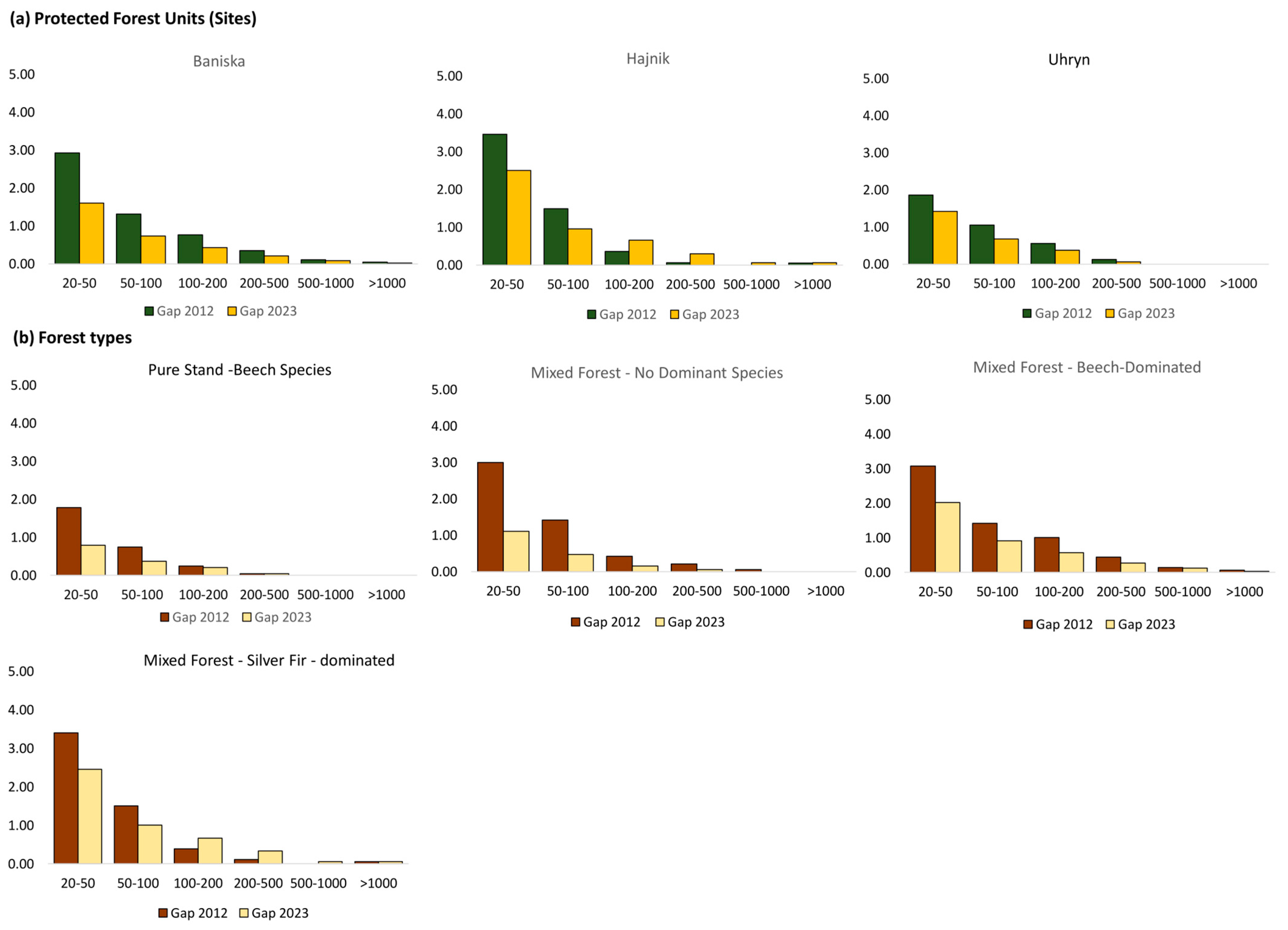
We characterized the gap size structure by examining the frequency distribution in discrete size classes. Regardless of the stratifications (site and forest type), the gap size distribution skewed to the right. Gaps frequently occurred in smaller size classes at 20–50 m2, followed by 50–100 m2 size classes. The frequency then further reduced along larger size classes (100–200 m2, 200–500 m2, 500–1000 m2) with fewer to no counts as approaching very large size classes (>1000 m2). Concomitantly, gap size frequency difference between 2012 and 2023 reveals that a decrease in gap frequency was prevalent in smaller gap size classes (20–50 m2, 50–100 m2, and 100–200 m2) (Table 4; Figure 3).
We tested for change in the GSFD proportion between years among sites and forest types using the chi-squared test for distribution. We found evidence of significant change for Hajnik ( ρ -value for x 2 ~0.04). Across forest types, the Mixed Forest Silver Fir-Dominated tested for significant change ( ρ -value for x 2 ~0.05). Among gap size categories, gap size classes > 100 m2 were the ones significantly contributing to changes in proportion, indicating a medium to large-scale disturbance.

3.3. Gap Size Probability Distribution

To find a plausible model that can explain the probability distribution of the gap size, we fitted it to four candidate models using maximum likelihood estimation [53]. Candidate models were compared according to their Akaike’s information criteria (AIC). Probability distribution models, log-normal, power-law, and exponential, fitted fairly except for Weibull (Table 5). We found out that the gap size in sites and forest type groups between periods assumed different distributions. Baniska and Uhryn consistently followed a log-normal distribution between periods. Meanwhile, Hajnik shifted from a log-normal to a power-law distribution, indicating the presence of some larger gaps for 2023, which we previously confirmed in a x 2 test for change in gap proportion. Meanwhile, forest types MFND and MFSFD transitioned from log-normal to power-law distribution, PSB transitioned from log-normal to exponential distribution, and MFBD remained in the log-normal distribution in the entire period. These transition patterns indicate that canopy gap dynamics vary across forest types, with log-normal distributions reflecting disturbance regimes dominated by small gaps, while transitions toward power-law behavior suggest the increasing influence of larger canopy disturbances in certain forest types.

3.4. Gap Size and Shape Metrics

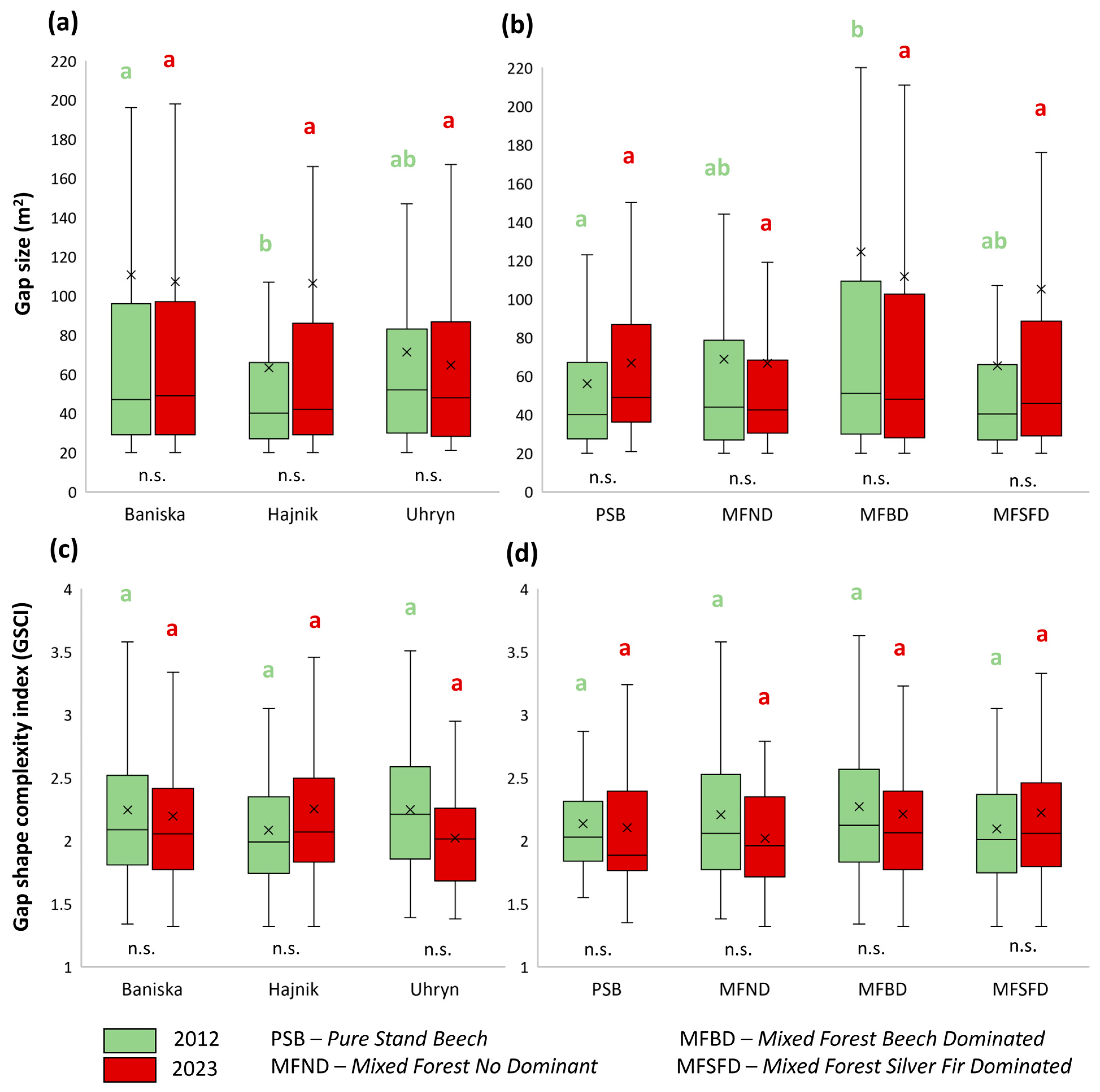
We found a significant difference in gap sizes between sites in 2012 ( ρ -value for H ~0.049), with Baniska showing a wider IQR and larger median gap size value. Contrastingly, Hajnik shows a narrow IQR and a smaller median value, and Uhryn is in the middle. Meanwhile, approaching 2023, the gaps tend to have similar sizes, characterized by larger median values (Figure 4a). We also found a significant difference in gap sizes between forest types in 2012 ( ρ -value for H ~0.004), with PSB showing smaller gap sizes in contrast to MFBD, which exhibited larger gap sizes and wider IQR. However, approaching 2023, the gap sizes among forest types tend to be similar and do not significantly differ from each other (Figure 4b).
Baniska, Hajnik, and Uhryn have mean GSCI values ranging from 2.08 to 2.24 (2012) and from 2.02 to 2.25 (2023), with Hajnik observed with an increased mean GSCI value (Figure 4c). Across forest types, the mean GSCI value range was 2.09–2.27 (2012) and 2.02–2.22 (2023) (Figure 4d). The range of mean values for site and forest types falls within the moderately irregular complexity category. However, the Wilcoxon rank sum test yielded a p-value > 0.05, indicating no significant difference in GSCI values between periods across sites and forest types (Figure 4c,d).

3.5. Gap Size and Shape Complexity

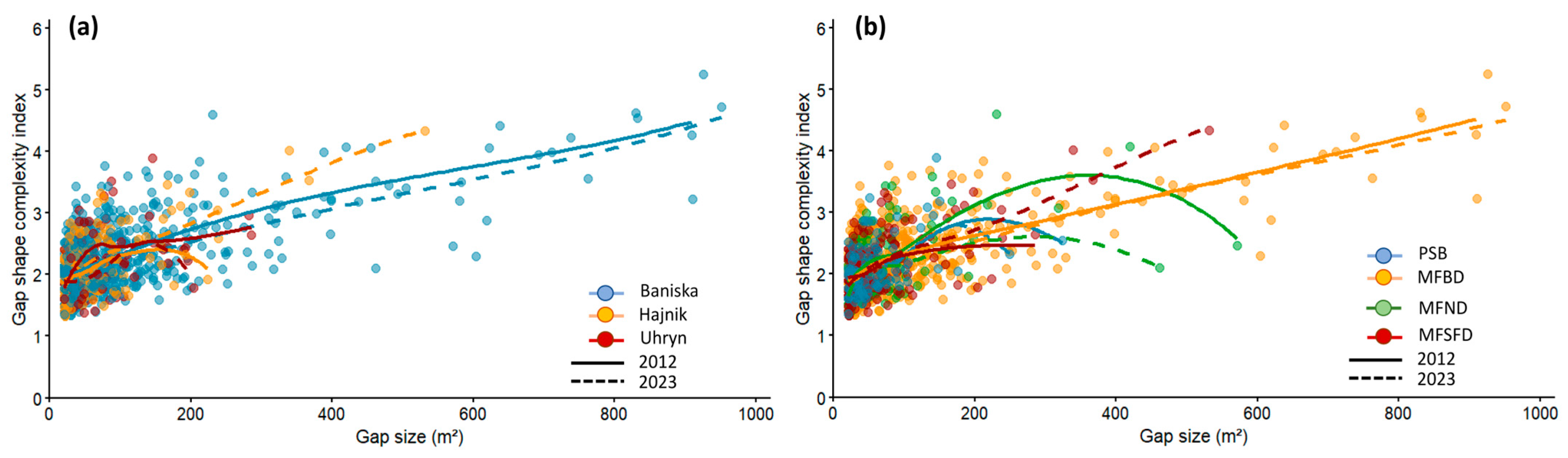
We also examined the relationship between the complexity of the gap shape and gap size using Kendall’s Tau (τ) method correlation analysis (Figure 5). Across sites and periods, Kendall’s τ ranges from 0.20 to 0.45 with q < 0.01 (Figure 5a). Across forest types and periods, Kendall’s τ ranges from 0.20 to 0.40 with q < 0.01 (Figure 5b). The association between gap size and shape complexity showed a positively monotonic, moderate level of correlation, indicating that shape complexity increases with gap size.

3.6. Gap Formation and Closure

By comparing canopy gap openings between 2012 and 2023, we identified four distinct processes that characterize gap formation and closure dynamics (Table 6). Some canopy gaps were formed from previously full canopy-covered areas, creating a new opening. Other gaps were formed as an extension of existing gaps, known as expanded gaps. Gaps may also persist and remain open for a very long period, known as persistent gaps. Lastly, we also observed gap closure or the recovery to a closed canopy. The rates and proportions of these distinct gap processes determine the gap dynamic status in a given area. Conditions were site-specific, Baniska was on recovering status with a gap closure percentage exceeding the opening percentage, with a balance of ~7%. Uhryn showed an equal percentage of opening and closing, no gain and no loss, with a balance of ~ 0, indicating a steady state. On the other hand, Hajnik was observed with 31% closing gaps and 69% opening gaps, with a balance of ~−39% indicating a site with a progressing canopy opening. In gap formation, the expanding type of opening was prevalent in Hajnik, while Baniska and Uhryn were dominated by newly created gaps.
Among forest types, we found a very pronounced recovering condition for MFND with a balance of ~40%, while PSB and MFBD were near steady-state with balances of 1% and 3%, respectively. Meanwhile, MFSFD showed a prevalence of openings, with a balance of ~−37% and gap formation dominantly driven by expansion (35%).

4. Discussion

This study provides insights into the dynamics of disturbance regimes and the restoration process through a progressive approach and with reference to methodological limitations in the past. The analysis of the gap features using a remote sensing approach addresses the limitations observed for the contemporary field-based method. This approach offered flexibility in the observation of gap dynamics at a wider spatial scale and a broader span of time. Across the literature, canopy gaps were defined by various height thresholds and area criteria. Hence, this study also takes into account the optimization of the canopy gap detection process through the selection of the height and gap size thresholds defining a canopy gap appropriate to the canopy stand structure. Most of the early field-based studies used fixed height thresholds [11,58,59]. Although these thresholds were derived from empirical observations, applying them at a larger spatial scale and at heterogonous stands with varying height, similar to our study site, tends to oversimplify canopy structural variability. The presence of different forest types by species composition contributed to the complexity; hence, we adapted stand-level relative height threshold determination. By doing so, we were able to determine the specific height cut-off based on the 1/3 of the stand threshold, avoiding the over-simplification of the stand variability that may result in over- and under-estimation of the canopy gaps in the stands.
Meanwhile, the determination of the lower gap size limit is as important as the former parameter, and the coupling of these two parameters ultimately defines the gaps for the detection process. A minimum gap size of 20 m2 was used for the consideration of the commonality of the use of the threshold value across the literature [31,41,60]. In the ecological context, the 20 m2 lower limit will exclude small branch gaps and natural canopy openings [60,61]. In the context of remote sensing, a very low limit can possibly result in the introduction of noise and the overestimation of gaps in the canopy gap detection process. The result of the sensitivity analysis indicates that while the selection of minimum gap-size threshold influences the number of detected gaps and their absolute size distributions, the relative patterns among sites and between years remain consistent (Table S2; Figure S1). Correlation analysis further showed a strong relationship between metrics derived from different thresholds (r = 0.96), indicating that the ecological interpretation of gap dynamics is robust to threshold selection (text after Figure S1 in Supplemental Materials).
We found notable trends in the proportion of the gaps, the number of gaps, and the size of the gaps across time. Reduction in the gap area proportion or gap percentage towards the final period was generally observed across sites and forest types within the 11-year monitoring period. This was accompanied by a 2/3 reduction in mean gap counts, ranging from 5.6 gaps ha−1 to 2.6 gaps ha−1 between sites and from 6.2 gaps ha−1 to 1.5 gaps ha−1 between forest types. These reductions in the proportion of the gaps and number of gaps are accompanied by increased mean gap size in the final period. These trends are similar to other studies conducted in forest ecosystems with either communal or unmanaged statuses [22,62]. A related study in a Beech-dominated forest of the Carpathians revealed similar patterns to our findings. The number of gaps from the initial to final period (2003–2013) reduced by 50%, the gap fraction decreased from 13.6% to 5.4%, and a strong decrease in the mean gap size was observed [62]. Similar trends were observed in coniferous forests, broadleaved forests, and mixed forests [22]. While there were differences in the values across forest types, their findings emphasized a general reduction in the forest gap area and number of gaps, but an increased size gap (mean gap area) between 2010 and 2016. These trends were observed in our study, and as supported by the findings of related studies, they could be explained by the homeostatic characteristic of a forest—the ability to recover after disturbance through its regeneration capacity with a general direction of a closing forest [63]; in the case of our study, the reduction in the gap area proportion across time. During this regeneration process, these trends can be explained by the fact that the number of gaps decreases over time due to the process of gap closure, primarily facilitated by the growth of advanced regeneration that achieves canopy position over time [64]. Smaller gaps close faster due to regeneration filling of the openings and the lateral crown expansion by surrounding canopy trees. Since frequent but smaller gaps close faster, the gap counts in a given area can decrease over time [65]. However, as the number of gaps reduces, gap size may increase due to the merging of other smaller gaps into larger gaps (coalescence) [66]. Another scenario is that gaps that did not close often continue to expand [3]. Considering the unmanaged and protected nature of the sampled area, it is also often expected that regeneration growth closes gaps in time, except for cases where natural disturbances drive the creation of gaps that exceed the recovery rate [67].
We examined further the characteristics of the gaps through their frequency distribution and found that the binned gap size frequency distribution shape was relatively stable regardless of site and forest types across time, even with the reduction in the number of gaps. The distribution can be described with a right-skewed shape, indicating frequent gap occurrence at smaller groups following the decreasing slopes towards the right, representing the large gap size group. This is similar to the result of the study in a multi-species lowland temperate forest in Poland, where binned distributions were compared between two periods (2015 and 2022), and their result indicated that frequencies were dominated by smaller size classes, although it was observed that the gap counts increased in each size class in the final monitoring period [31]. Related studies found that disturbance regimes were frequently dominated by fine-scale disturbances, creating small openings, and with rare occurrences of large-scale disturbances, but at extensive openings [67,68]. Gaps predominantly occur as fine-scale processes of smaller size (20–50 m2), which can be associated with mortality of smaller trees and/or branch falls and related mechanical damages caused by, but not limited to, ice loading and wind gusts [69,70]. Artifacts of disturbances with gap sizes approximately ranging from 50 to 100 m2 and from 100 to 200 m2 follow the order of frequency, which can be caused by a single tree failure, depending on the species and tree age or size. Medium to larger-scale disturbances of spatial scales (200–500 m2, 500–1000 m2, and >1000 m2) [48] typically cause multiple tree failures. For instance, such disturbances occasionally happen in the Beskid Sądecki range of the Western Carpathian mountains [71], where episodic cases of major windthrow, storms, and mass movements (landslide and snow avalanches) were indicated as possible drivers, especially of large openings in the study area [72,73].
The GSFD was further analyzed by fitting to several probability distribution models. Some studies determined that GSFD often follows a power-law distribution [22,74], but deviations from this pattern can occur [75]. Thus, instead of fitting directly to a power-law model, the gap size data were fitted to different models under the heavy-tailed family. The outcome indicated that the probability distributions of gap sizes were not exclusively tied to power-law, but some were better fitted with log-normal and exponential models. Moreover, further skewing of the distribution due to the increasing occurrence of larger gaps resulted in a model shifting across the observed time period from log-normal to power-law. On the other hand, the shift from log-normal to exponential indicated a further narrowing of the range of gap sizes, as in the case of the PSB. Although a power law is typically expected as a model of gap size distributions, other models that occurred in the present study are not illogical since the distribution is scale-dependent. Smaller study areas and finer thresholds tend to under-sample rare large gaps, steepening the observed GSFD and potentially favoring exponential fits, whereas landscape-scale analyses that capture the tail often support heavier-tailed forms [21,75]. In general, a log-normal to power-law distribution trend was observed, indicating a small gap-phase dynamics in the earlier stage of the monitoring, followed by the presence of larger gaps at the latter stage.
Here we present the parameter estimates obtained from the fitted distribution models. The scaling parameter α is 1.97 at a site and 1.95–2.12 among forest types, which lies within the range reported for a variety of ecosystems (approximately 1.1–3.1) [22]. Related studies have suggested that values around α ≈ 2 may indicate differences in disturbance regimes, with lower values sometimes associated with relatively larger disturbance events and higher values with smaller-scale gap dynamics. In this context, the α values observed in our study are broadly consistent with patterns reported in temperate forest ecosystems, but they should be interpreted as general descriptors of gap-size scaling rather than strict thresholds defining disturbance regimes [32]. Other distribution models follow the same trend in which patterns were found to have similarity when compared to other sites. For example, log-normal fits in the studied forests yielded μ values between 3.8 and 4.1 (log10 m2), corresponding to median gap sizes of ~45–60 m2. These ranges are consistent with previous reports [68,76] of log-normal canopy gap distributions in temperate forests (μ ≈ 1.6–2.5; σ ≈ 0.3–0.8). In the same way, the exponential fit for Pure Stand Beech in 2023 yielded a rate parameter β = 0.01, equivalent to a median gap size of ~69 m2, which falls within the 20–100 m2 range commonly reported in temperate forests where small gaps dominate and the gap-size distribution declines rapidly with increasing gap size [21,62]. Despite differences in species composition and structure, many ecosystems respond to disturbances in relatively and categorically similar ways. This consistency reflects shared underlying mechanisms—such as feedback loops and resilience—that shape ecosystem dynamics. Forest biomes from temperate to tropical regions exhibit comparable patterns driven by these complex system properties [77]. Different forest ecosystems often show similar gap probability distributions because they are shaped by the same or similar underlying ecological processes. Disturbances such as tree falls and mortality events create canopy gaps that follow consistent statistical patterns, and gap-size distributions converge across forests, reflecting shared ecological mechanisms [78].
Meanwhile, we found that the interplay of these distribution models highlights the complexity of forest ecosystems and reveals how various factors, such as disturbance history and environmental conditions, play critical roles in shifts in gap size distributions across time. The transitions between log-normal, power-law, and exponential distributions in our data can also be explained through the temporal dynamics of gap formation and closure. Environmental stresses and disturbances contribute to canopy dynamics and gap size distributions [79]. Their findings suggest that ecosystems subjected to frequent disturbances may exhibit power-law characteristics due to the predominance of smaller gaps, while more stable environments may display log-normal characteristics reflecting more uniform mortality and regeneration patterns. This is evident from the result of our study, such as the Hajnik site, which was observed with increased disturbance for the final period, reflecting a shift from log-normal to power-law distribution.
In the next stage, an analysis of how complex the shapes of the formed gaps are, and if they differ between forest types and across time, was conducted. In the study, GSCI values ranged from 2.02 to 2.25 across sites and from 2.02 to 2.27 across forest types and did not significantly change across time. These values do not deviate much from the values in other studies, e.g., 2.64 for a deciduous woodland and 2.3 for unmanaged beech forests [12]. The stable GSCI values over time suggest that the studied forests maintain a relatively steady balance in gap formation and closure. This consistency implies that processes such as mortality, competition, and natural disturbances operate regularly [80]. Meanwhile, the small variation from values reported in other studies also points to shared disturbance patterns across temperate forests. The close similarity of GSCI values across temperate forest types suggests that gap dynamics are shaped by shared ecological mechanisms. These patterns likely reflect common biotic and abiotic factors influencing growth and mortality and resulting in comparable gap formation processes. Such consistency supports cross-comparison among forests and strengthens the generalizability of findings in forest ecology [12].
While the values seemed similar across sites and forest types, it is worth looking at the range of values for a fir-dominated forest. The reported value is typically in the range of ~1.2–1.6 [2]. However, in the MFSFD, GSCI values ranged from approximately 2.09 to 2.22, indicating higher complexity beyond the expected range. We observed that in MFSFD, gap distribution shifted from log-normal to power-law, indicating the presence of larger gaps in 2023. Larger gaps are associated with more complex shapes, which is an observable trend in our gap size and shape relationship study. And in an ecological context, these complex structures commonly develop in disturbed forests, where fallen trees create diverse gap patterns that support varied regeneration strategies [81]. A previous study reported that Silver Fir forests have higher vulnerability to disturbance due to their shade tolerance and slower growth rates and recovery, leading to an accumulation of complex gap structures as trees fall and gaps are filled by various species over time [82].
We also looked into the dynamics of the gap sizes and their corresponding shape because gaps are dynamic entities that increase or decrease in size and complexity based on ecological interactions and environmental conditions as an outcome of a cumulative process over time [83]. The result of the correlation analysis indicated a monotonic moderate positive correlation between gap size and shape complexity. We found that regardless of the site factor and forest types, the geometry of the gap tended to be more complex as the gap size increased. This finding was supported by the findings of a related study [21], where larger canopy gaps exhibited greater boundary complexity (higher shape index) across boreal, deciduous, and mixed wood forests, consistent with the idea that gap shape becomes increasingly complex as gap size increases. Another study conducted in a multi-species temperate forest holds the same observation [31]. This means that larger gaps often exhibit more complex shapes as a result of ecological interactions and the conditions created by disturbances. The intensity and frequency of disturbances that create gaps can lead to irregular shapes and varying sizes. While the claim of specific GSCI values was not directly supported [2], it is widely acknowledged that disturbances drive variation in gap characteristics and complexity. Process-wise, the expansion of single gaps and the coalescence of smaller gaps over time into single larger gaps contribute to the increased shape complexity [66]. Related study indicated that old-growth forests display considerable variation in their gap-phase dynamics, with gap size and structure strongly influencing overall complexity [40]. Larger gaps often support a wider range of species and create diverse microhabitats, which can lead to higher GSCI values.
Lastly, the process of gap formation and the recovery of the canopy over a decade was analyzed. By contrasting the binary canopy gaps between the initial and final period, four important gap phases were determined. Recovered canopy (closed), persistent gap, larger gap by expansion from a single existing smaller gap or by coalescence of two or more smaller gaps, and newly created gap. Other studies identified that gap expansion is the dominant process in canopy gap dynamics [29]. However, our study showed that the dominant process in these dynamics could be either expansion or new gap creation. We tried to find a pattern among the groups; nonetheless, no strong justification can be established for why expansion and new gaps appeared to be random. It is a noteworthy observation that in a more disturbed site (Hajnik), we found a high percentage (~38%) of expanding gaps compared to new gaps (~12%). Meanwhile, in a steady-state forest site like Uhryn (1:1–opening and closing), the percentage of the new gaps was higher compared to expanded gaps. One possible explanation is that in the absence of large-scale disturbance drivers, canopy opening can be driven by fine-scale disturbance, such as branch failure or individual tree fall, thereby creating new gaps. Meanwhile, under large-scale disturbance, a persistent gap can act as a vulnerable spot for canopy failure and could therefore result in high expansion percentage.
In general, the site and forest type groupings have a higher percentage of closed gaps over the 11 years, indicating a recovering forest. The resilience of forests, characterized by their ability to recover from disturbances, is closely tied to their homeostatic potential. This trend is evident in a related study [84] which found that significantly large and medium gaps were closing over time in secondary forests. Gaps formed by disturbances in forests act as important sites for regeneration and recovery. Disturbances create openings that surrounding trees gradually fill in, highlighting the dynamic relationship between disturbance and forest renewal [27]. However, an alternative scenario can happen where larger disturbances are characterized by a higher percentage of canopy opening compared to closing, resulting in a negative balance. Recurring disturbances can significantly influence the homeostatic mechanisms of forest ecosystems. Consequently, intense disturbances that create large gaps may allow certain species to thrive due to increased light availability, changing species composition [85].

5. Conclusions

A comprehensive yet site-tailored approach to the study of forest gap dynamics is necessary for a deeper understanding of disturbance regimes and the restoration process in a protected forest. In this study, we applied multiple metrics and used bi-temporal data with consideration of stand-level variations in the canopy gap detection process. This provides more robust quantification of canopy gap features and more comprehensive elucidation of their dynamics over a decade in three strictly protected temperate forests in the Carpathian Mountains. The results not only exhibited consistency with the findings of previous related studies but also showcased site-specificity. Our observations indicated that the gap profile changes depend on the level of severity of the disturbance. In most disturbed areas, canopy gap dynamics were characterized by expanded gaps, whereas in less disturbed areas, governed by fine-scale disturbance, were dominated by new openings. However, despite the varying intensity and the repetitive nature of the disturbances, the homeostatic capacity of the studied forest consequently converges back to gap trends that were identical across forest ecosystems. In the studied area, we found a general reduction in areas with gaps over time, accompanied by smaller gap numbers but larger gap sizes. Yet, regardless of these changes in gap properties, the GSFD structure remained the same, following a right-skewed curve shape and variably fits to exponential, log-normal, or power-law models. This is indicative of the dominance of fine-scale disturbances except for the occasional cases of disturbances that caused proportional shifts. The obtained results also demonstrated pronounced gap-shape plasticity, evidenced by the systematic increase in shape complexity with expanding gap size.
The findings of this study provide valuable guidance for the management of protected forests, particularly in the context of close-to-nature and restoration-oriented strategies. By demonstrating how gap size and shape influence regeneration pathways and ecological processes, the results support management approaches that mimic natural disturbance regimes rather than rely on uniform, large-scale interventions. The observed gap dynamics could inform management on how natural restoration takes place under the scenario of recurring natural disturbances. Lastly, the output of this study can contribute to the pool of existing knowledge of canopy gap dynamic studies by providing localized information based on high mountain forest ecosystems in Poland.

Supplementary Materials

The following supporting information can be downloaded at: https://www.mdpi.com/article/10.3390/rs18071045/s1, Section S1: Result of the assessment for systematic vertical bias after vertical height transformation using Nearest-neighbor ground elevation comparison. Section S2: Sensitivity Analysis. Table S1. Changes in the Gap Metrics per lower size limit threshold 1, 10, 20 adjustments. Figure S1. Boxplot of gap area tested at three threshold levels 1, 10, 20 showing similar patterns. Section S3: Report on uncertainty estimates. Table S2. Estimated parameters of fitted distributions for tree size distributions by forest type and site. Parameter uncertainty is reported as 95% confidence intervals obtained from bootstrap resampling.

Author Contributions

Conceptualization, G.M. and S.K.; methodology, G.M., S.K. and J.M.; software, G.M. and J.M.; validation, S.K.; formal analysis, G.M. and S.K.; investigation, G.M. and S.K.; resources, G.M., S.K. and J.M.; data curation, G.M. and S.K.; writing—original draft preparation, G.M.; writing—review and editing, G.M. and S.K.; visualization, G.M. and J.M.; supervision, S.K.; project administration, G.M.; funding acquisition, G.M. and S.K. All authors have read and agreed to the published version of the manuscript.

Funding

This research received no external funding.

Data Availability Statement

The data presented in this study are available on request from the corresponding author due to legal and ethical restrictions.

Conflicts of Interest

The authors declare no conflicts of interest.

Abbreviations

The following abbreviations are used in this manuscript:
ALSAerial Laser Scanning
LiDARLight detection and ranging
TLETerrestrial laser scanning
GSFDGap size frequency distribution
GSCIGap shape complexity index
PSBPure Stand Beech
MFBDMixed Forest Beech-Dominated
MFSFDMixed Forest Silver Fir-Dominated
MFNDMixed Forest No Dominant

References

  1. Fischer, A.; Marshall, P.; Camp, A. Disturbances in Deciduous Temperate Forest Ecosystems of the Northern Hemisphere: Their Effects on Both Recent and Future Forest Development. Biodivers. Conserv. 2013, 22, 1863–1893. [Google Scholar] [CrossRef] [Scilit]
  2. Nagel, T.A.; Svoboda, M. Gap Disturbance Regime in an Old-Growth Fagus-Abies Forest in the Dinaric Mountains, Bosnia-Herzegovina. Can. J. For. Res. 2008, 38, 2728–2737. [Google Scholar] [CrossRef] [Scilit]
  3. Whitmore, T.C. Canopy Gaps and the Two Major Groups of Forest Trees. Ecology 1989, 70, 536–538. [Google Scholar] [CrossRef] [Scilit]
  4. Abd Latif, Z.; Blackburn, G.A. The Effects of Gap Size on Some Microclimate Variables during Late Summer and Autumn in a Temperate Broadleaved Deciduous Forest. Int. J. Biometeorol. 2010, 54, 119–129. [Google Scholar] [CrossRef] [Scilit] [PubMed]
  5. Wagner, S.; Fischer, H.; Huth, F. Canopy Effects on Vegetation Caused by Harvesting and Regeneration Treatments. Eur. J. For. Res. 2011, 130, 17–40. [Google Scholar] [CrossRef] [Scilit]
  6. Johnson, D.J.; Magee, L.; Pandit, K.; Bourdon, J.; Broadbent, E.N.; Glenn, K.; Kaddoura, Y.; Machado, S.; Nieves, J.; Wilkinson, B.E.; et al. Canopy Tree Density and Species Influence Tree Regeneration Patterns and Woody Species Diversity in a Longleaf Pine Forest. For. Ecol. Manag. 2021, 490, 119082. [Google Scholar] [CrossRef] [Scilit]
  7. Jucker, T. Deciphering the Fingerprint of Disturbance on the Three-dimensional Structure of the World’s Forests. New Phytol. 2022, 233, 612–617. [Google Scholar] [CrossRef] [Scilit] [PubMed]
  8. Kern, C.C.; Burton, J.I.; Raymond, P.; D’Amato, A.W.; Keeton, W.S.; Royo, A.A.; Walters, M.B.; Webster, C.R.; Willis, J.L. Challenges Facing Gap-Based Silviculture and Possible Solutions for Mesic Northern Forests in North America. Forestry 2017, 90, 4–17. [Google Scholar] [CrossRef] [Scilit]
  9. Larsen, J.B.; Angelstam, P.; Bauhus, J.; Carvalho, J.F.; Diaci, J.; Dobrowolska, D.; Gazda, A.; Gustafsson, L.; Krumm, F.; Knoke, T.; et al. Closer-to-Nature Forest Management; From Science to Policy; European Forest Institute: Barcelona, Spain, 2022. [Google Scholar]
  10. Naka, K. Community Dynamics of Evergreen Broadleaf Forests in Southwestern Japan. I. Wind Damaged Trees and Canopy Gaps in an Evergreen Oak Forest. Bot. Mag. Tokyo 1982, 95, 385–399. [Google Scholar] [CrossRef] [Scilit]
  11. Brokaw, N.V.L. Gap-Phase Regeneration in a Tropical Forest. Ecology 1985, 66, 682–687. [Google Scholar] [CrossRef] [Scilit]
  12. Koukoulas, S.; Blackburn, G.A. Quantifying the Spatial Properties of Forest Canopy Gaps Using LiDAR Imagery and GIS. Int. J. Remote Sens. 2004, 25, 3049–3072. [Google Scholar] [CrossRef] [Scilit]
  13. Dietmaier, A.; McDermid, G.J.; Rahman, M.M.; Linke, J.; Ludwig, R. Comparison of LiDAR and Digital Aerial Photogrammetry for Characterizing Canopy Openings in the Boreal Forest of Northern Alberta. Remote Sens. 2019, 11, 1919. [Google Scholar] [CrossRef] [Scilit]
  14. Chung, C.-H.; Wang, J.; Deng, S.-L.; Huang, C. Analysis of Canopy Gaps of Coastal Broadleaf Forest Plantations in Northeast Taiwan Using UAV Lidar and the Weibull Distribution. Remote Sens. 2022, 14, 667. [Google Scholar] [CrossRef] [Scilit]
  15. Brunig, E.F. Some Further Evidence on the Amount of Damage Attributed to Lightning and Wind-Throw in Shorea Albida-Forest in Sarawak. Commonw. For. Rev. 1973, 52, 260–265. [Google Scholar]
  16. Souza, C. Mapping Forest Degradation in the Eastern Amazon from SPOT 4 through Spectral Mixture Models. Remote Sens. Environ. 2003, 87, 494–506. [Google Scholar] [CrossRef] [Scilit]
  17. Dalagnol, R.; Phillips, O.L.; Gloor, E.; Galvão, L.S.; Wagner, F.H.; Locks, C.J.; Aragão, L.E.O.C. Quantifying Canopy Tree Loss and Gap Recovery in Tropical Forests under Low-Intensity Logging Using VHR Satellite Imagery and Airborne LiDAR. Remote Sens. 2019, 11, 817. [Google Scholar] [CrossRef] [Scilit]
  18. Östersund, M.; Honkavaara, E.; Oliveira, R.A.; Näsi, R.; Hakala, T.; Koivumäki, N.; Pelto-Arvo, M.; Tuviala, J.; Nevalainen, O.; Lyytikäinen-Saarenmaa, P. Exploring Forest Changes in an Ips typographus L. Outbreak Area: Insights from Multi-Temporal Multispectral UAS Remote Sensing. Eur. J. For. Res. 2024, 143, 1871–1892. [Google Scholar] [CrossRef] [Scilit]
  19. White, J.C.; Tompalski, P.; Coops, N.C.; Wulder, M.A. Comparison of Airborne Laser Scanning and Digital Stereo Imagery for Characterizing Forest Canopy Gaps in Coastal Temperate Rainforests. Remote Sens. Environ. 2018, 208, 1–14. [Google Scholar] [CrossRef] [Scilit]
  20. LaRue, E.; Wagner, F.; Fei, S.; Atkins, J.; Fahey, R.; Gough, C.; Hardiman, B. Compatibility of Aerial and Terrestrial LiDAR for Quantifying Forest Structural Diversity. Remote Sens. 2020, 12, 1407. [Google Scholar] [CrossRef] [Scilit]
  21. Goodbody, T.R.H.; Tompalski, P.; Coops, N.C.; White, J.C.; Wulder, M.A.; Sanelli, M. Uncovering Spatial and Ecological Variability in Gap Size Frequency Distributions in the Canadian Boreal Forest. Sci. Rep. 2020, 10, 6069. [Google Scholar] [CrossRef] [Scilit]
  22. Rodes-Blanco, M.; Ruiz-Benito, P.; Silva, C.A.; García, M. Canopy Gap Patterns in Mediterranean Forests: A Spatio-Temporal Characterization Using Airborne LiDAR Data. Landsc. Ecol. 2023, 38, 3427–3442. [Google Scholar] [CrossRef] [Scilit]
  23. Gaulton, R.; Malthus, T.J. LiDAR Mapping of Canopy Gaps in Continuous Cover Forests: A Comparison of Canopy Height Model and Point Cloud-Based Techniques. Int. J. Remote Sens. 2010, 31, 1193–1211. [Google Scholar] [CrossRef] [Scilit]
  24. St-Onge, B.; Vepakomma, U.; Sénécal, J.-F.; Kneeshaw, D.; Doyon, F. Canopy Gap Detection and Analysis with Airborne Laser Scanning. In Forestry Applications of Airborne Laser Scanning; Maltamo, M., Næsset, E., Vauhkonen, J., Eds.; Managing Forest Ecosystems; Springer: Dordrecht, The Netherlands, 2014; Volume 27, pp. 419–437. [Google Scholar]
  25. Leclère, L.; Latte, N.; Candaele, R.; Ligot, G.; Lejeune, P. Estimation of Within-Gap Regeneration Height Growth in Managed Temperate Deciduous Forests Using Bi-Temporal Airborne Laser Scanning Data. Ann. For. Sci. 2024, 81, 36. [Google Scholar] [CrossRef] [Scilit]
  26. Vehmas, M.; Packalén, P.; Maltamo, M.; Eerikäinen, K. Using airborne laser scanning data for detecting canopy gaps and their understory type in mature boreal forest. Ann. For. Sci. 2011, 68, 825–835. [Google Scholar] [CrossRef] [Scilit]
  27. Vepakomma, U.; St-Onge, B.; Kneeshaw, D. Response of a Boreal Forest to Canopy Opening: Assessing Vertical 850 and Lateral Tree Growth with Multi-Temporal Lidar Data. Ecol. Appl. 2011, 21, 99–121. [Google Scholar] [CrossRef] [Scilit] [PubMed]
  28. Asner, G.P.; Kellner, J.R.; Kennedy-Bowdoin, T.; Knapp, D.E.; Anderson, C.; Martin, R.E. Forest Canopy Gap Distributions in the Southern Peruvian Amazon. PLoS ONE 2013, 8, e60875. [Google Scholar] [CrossRef] [Scilit]
  29. Krüger, K.; Senf, C.; Jucker, T.; Pflugmacher, D.; Seidl, R. Gap Expansion Is the Dominant Driver of Canopy Openings in a Temperate Mountain Forest Landscape. J. Ecol. 2024, 112, 1501–1515. [Google Scholar] [CrossRef] [Scilit]
  30. Dalagnol, R.; Wagner, F.H.; Galvão, L.S.; Streher, A.S.; Phillips, O.L.; Gloor, E.; Pugh, T.A.M.; Ometto, J.P.H.B.; Aragão, L.E.O.C. Large-Scale Variations in the Dynamics of Amazon Forest Canopy Gaps from Airborne Lidar Data and Opportunities for Tree Mortality Estimates. Sci. Rep. 2021, 11, 1388. [Google Scholar] [CrossRef] [Scilit]
  31. Mielcarek, M.; Kurpiewska, S.; Guderski, K.; Dobrowolska, D.; Zin, E.; Kuberski, Ł.; Erfanifard, Y.; Stereńczak, K. Remote Sensing of Forest Gap Dynamics in the Białowieża Forest: Comparison of Multitemporal Airborne Laser Scanning and High-Resolution Aerial Imagery Point Clouds. Remote Sens. 2025, 17, 1149. [Google Scholar] [CrossRef] [Scilit]
  32. Fisher, J.I.; Hurtt, G.C.; Thomas, R.Q.; Chambers, J.Q. Clustered Disturbances Lead to Bias in Large-scale Estimates Based on Forest Sample Plots. Ecol. Lett. 2008, 11, 554–563. [Google Scholar] [CrossRef] [Scilit]
  33. Spies, T.A.; Johnson, K.N.; Burnett, K.M.; Ohmann, J.L.; McComb, B.C.; Reeves, G.H.; Bettinger, P.; Kline, J.D.; Garber-Yonts, B. Cumulative ecological and socioeconomic effects of forest policies in coastal Oregon. Ecol. Appl. 2007, 17, 5–17. [Google Scholar] [CrossRef] [Scilit]
  34. Guyon, L.; Strassman, A.C.; Oines, A.; Meier, A.; Thomsen, M.; Sattler, S.R.; DeJager, N.R.; Hoy, E.E.; Vandermyde, B.; Cosgriff, R. Forest Canopy Gap Dynamics: Quantifying Forest Gaps and Understanding Gap—Level Forest Regeneration in Upper Mississippi River Floodplain Forests; USGS: Reston, VA, USA, 2023; p. 73.
  35. Gorgens, E.B.; Keller, M.; Jackson, T.; Marra, D.M.; Reis, C.R.; De Almeida, D.R.A.; Coomes, D.; Ometto, J.P. Out of 832 Steady State: Tracking Canopy Gap Dynamics across Brazilian Amazon. Biotropica 2023, 55, 755–766+833. [Google Scholar] [CrossRef] [Scilit]
  36. Wu, C.-D.; Cheng, C.-C.; Chang, C.-C.; Lin, C.; Chang, K.-C.; Chuang, Y.-C. Gap Shape Classification Using Landscape Indices and Multivariate Statistics. Sci. Rep. 2016, 6, 38217. [Google Scholar] [CrossRef] [Scilit] [PubMed]
  37. Zhang, B.; Fischer, F.J.; Coomes, D.A.; Jucker, T. Logging Leaves a Fingerprint on the Number, Size, Spatial Configuration and Geometry of Tropical Forest Canopy Gaps. Biotropica 2023, 55, 354–367. [Google Scholar] [CrossRef] [Scilit]
  38. Solano, F.; Modica, G.; Praticò, S.; Box, O.F.; Piovesan, G. Unveiling the Complex Canopy Spatial Structure of a Mediterranean Old-Growth Beech (Fagus sylvatica L.) Forest from UAV Observations. Ecol. Indic. 2022, 138, 108807. [Google Scholar] [CrossRef] [Scilit]
  39. Reis, C.R.; Jackson, T.D.; Gorgens, E.B.; Dalagnol, R.; Jucker, T.; Nunes, M.H.; Ometto, J.P.; Aragão, L.E.O.C.; Rodriguez, L.C.E.; Coomes, D.A. Forest Disturbance and Growth Processes Are Reflected in the Geographical Distribution of Large Canopy Gaps across the Brazilian Amazon. J. Ecol. 2022, 110, 2971–2983. [Google Scholar] [CrossRef] [Scilit]
  40. Bottero, A.; Garbarino, M.; Dukic, V.; Govedar, Z.; Lingua, E.; Nagel, T.; Motta, R. Gap-Phase Dynamics in the Old-Growth Forest of Lom, Bosnia and Herzegovina. Silva Fenn. 2011, 45, 76. [Google Scholar] [CrossRef] [Scilit]
  41. Hobi, M.L.; Commarmot, B.; Bugmann, H. Pattern and Process in the Largest Primeval Beech Forest of Europe (Ukrainian C Arpathians). J. Veg. Sci. 2015, 26, 323–336. [Google Scholar] [CrossRef] [Scilit]
  42. Główny Urząd Geodezji i Kartografii (GUGiK). Nazwa Zbioru Danych [ALS Data]. 2023. Available online: https://mapy.geoportal.gov.pl/imap/Imgp_2.html?gpmap=gp0 (accessed on 15 December 2023).
  43. R Core Team. R: A Language and Environment for Statistical Computing, Version 4.5.1; R Foundation for Statistical Computing: Vienna, Austria, 2025.
  44. ArcGIS Pro, Version 3.5.2; Esri: Redlands, CA, USA, 2023.
  45. General Directorate of State Forests and Statistics Poland. Forest Data for Poland; GUS: Warshaw, Poland, 2025. [Google Scholar]
  46. Dyba, K.; Nowosad, J. Rgugik: Search and Retrieve Spatial Data from the Polish Head Office of Geodesy and Cartography in R. J. Open Source Softw. 2021, 6, 2948. [Google Scholar] [CrossRef] [Scilit]
  47. American Society for Photogrammetry and Remote Sensing. ASPRS Positional Accuracy Standards for Digital Geospatial Data; American Society for Photogrammetry and Remote Sensing: Baton Rouge, LA, USA, 2015; Volume 81, pp. 1–26. [Google Scholar] [CrossRef] [Scilit]
  48. Roussel, J.-R.; Auty, D. LidR: Airborne LiDAR Data Manipulation and Visualization for Forestry Applications. Available online: https://rdrr.io/cran/lidR/ (accessed on 15 December 2025).
  49. Dalponte, M.; Coomes, D.A. Tree-Centric Mapping of Forest Carbon Density from Airborne Laser Scanning and Hyperspectral Data. Methods Ecol. Evol. 2016, 7, 1236–1245. [Google Scholar] [CrossRef] [Scilit]
  50. Rugani, T.; Diaci, J.; Hladnik, D. Gap Dynamics and Structure of Two Old-Growth Beech Forest Remnants in Slovenia. PLoS ONE 2013, 8, e52641. [Google Scholar] [CrossRef] [Scilit]
  51. Garbarino, M.; Borgogno Mondino, E.; Lingua, E.; Nagel, T.A.; Dukić, V.; Govedar, Z.; Motta, R. Gap Disturbances and Regeneration Patterns in a Bosnian Old-Growth Forest: A Multispectral Remote Sensing and Ground-Based Approach. Ann. For. Sci. 2012, 69, 617–625. [Google Scholar] [CrossRef] [Scilit]
  52. Silva, C.A.; Valbuena, R.; Pinagé, E.R.; Mohan, M.; De Almeida, D.R.A.; North Broadbent, E.; Jaafar, W.S.W.M.; De Almeida Papa, D.; Cardil, A.; Klauberg, C. ForestGap R: An r Package for Forest Gap Analysis from Canopy Height Models. Methods Ecol. Evol. 2019, 10, 1347–1356. [Google Scholar] [CrossRef] [Scilit]
  53. Pearson, K.X. On the Criterion That a given System of Deviations from the Probable in the Case of a Correlated System of Variables Is Such That It Can Be Reasonably Supposed to Have Arisen from Random Sampling. Lond. Edinb. Dublin Philos. Mag. J. Sci. 1900, 50, 157–175. [Google Scholar] [CrossRef] [Scilit]
  54. Fisher, R.A. On the Interpretation of χ2 from Contingency Tables, and the Calculation of P. J. R. Stat. Soc. 1922, 85, 87. [Google Scholar] [CrossRef] [Scilit]
  55. Bolker, B.M. Ecological Models and Data in R; Princeton University Press: Princeton, NJ, USA, 2008. [Google Scholar]
  56. Mann, H.B.; Whitney, D.R. On a Test of Whether One of Two Random Variables Is Stochastically Larger than the Other. Ann. Math. Stat. 1947, 18, 50–60. [Google Scholar] [CrossRef] [Scilit]
  57. Kendall, M.G. A New Measure of Rank Correlation. Biometrika 1938, 30, 81. [Google Scholar] [CrossRef] [Scilit]
  58. Nakashizuka, T.; Numata, M. Regeneration Process of Climax Beech Forests I: Structure of a Beech Forest with Sasa Understory. Jpn. J. Ecol. 1982, 32, 57–67. [Google Scholar]
  59. Nakashizuka, T. Regeneration Process of Climax Beech Forests IV: Gap Formation. Jpn. J. Ecol. 1984, 38, 62–66. [Google Scholar]
  60. Dobrowolska, D.; Piasecka, Ż.; Kuberski, Ł.; Stereńczak, K. Canopy Gap Characteristics and Regeneration Patterns in the Białowieża Forest Based on Remote Sensing Data and Field Measurements. For. Ecol. Manag. 2022, 511, 120123. [Google Scholar] [CrossRef] [Scilit]
  61. Brokaw, N.V.L. The Definition of Treefall Gap and Its Effect on Measures of Forest Dynamics. Biotropica 1982, 14, 158. [Google Scholar] [CrossRef] [Scilit]
  62. Feldmann, E.; Drößler, L.; Hauck, M.; Kucbel, S.; Pichler, V.; Leuschner, C. Canopy Gap Dynamics and Tree Understory Release in a Virgin Beech Forest, Slovakian Carpathians. For. Ecol. Manag. 2018, 415–416, 38–46. [Google Scholar] [CrossRef] [Scilit]
  63. Stevens-Rumann, C.S.; Kemp, K.B.; Higuera, P.E.; Harvey, B.J.; Rother, M.T.; Donato, D.C.; Morgan, P.; Veblen, T.T. 919 Evidence for Declining Forest Resilience to Wildfires under Climate Change. Ecol. Lett. 2018, 21, 243–252+920. [Google Scholar] [CrossRef] [Scilit] [PubMed]
  64. Hunter, M.O.; Keller, M.; Morton, D.; Cook, B.; Lefsky, M.; Ducey, M.; Saleska, S.; De Oliveira, R.C.; Schietti, J. 922 Structural Dynamics of Tropical Moist Forest Gaps. PLoS ONE 2015, 10, e0132144. [Google Scholar] [CrossRef] [Scilit] [PubMed]
  65. Lu, D.; Zhu, J.; Sun, Y.; Hu, L.; Zhang, G. Gap Closure Process by Lateral Extension Growth of Canopy Trees and 925 Its Effect on Woody Species Regeneration in a Temperate Secondary Forest, Northeast China. Silva Fenn. 2015, 49, 926. [Google Scholar] [CrossRef] [Scilit]
  66. Worrall, J.J.; Lee, T.D.; Harrington, T.C. Forest Dynamics and Agents That Initiate and Expand Canopy Gaps in Picea–Abies Forests of Crawford Notch, New Hampshire, USA. J. Ecol. 2005, 93, 178–190. [Google Scholar] [CrossRef] [Scilit]
  67. Yamamoto, S.-I. Forest Gap Dynamics and Tree Regeneration. J. For. Res. 2000, 5, 223–229. [Google Scholar] [CrossRef] [Scilit]
  68. Runkle, J.R. Patterns of Disturbance in Some Old-Growth Mesic Forests of Eastern North America. Ecology 1982, 63, 1533–1546. [Google Scholar] [CrossRef] [Scilit]
  69. Jaloviar, P.; Sedmáková, D.; Pittner, J.; Jarčušková Danková, L.; Kucbel, S.; Sedmák, R.; Saniga, M. Gap Structure and Regeneration in the Mixed Old-Growth Forests of National Nature Reserve Sitno, Slovakia. Forests 2020, 11, 81. [Google Scholar] [CrossRef] [Scilit]
  70. Strzyżowski, D. The Role of Topography, Canopy Gaps, and Forest Edges in the Distribution of Windthrow Damage in the Western Tatra Mountains, Poland. Geogr. Pol. 2019, 92, 173–187. [Google Scholar] [CrossRef] [Scilit]
  71. Ochtyra, A. Forest Disturbances in Polish Tatra Mountains for 1985–2016 in Relation to Topography, Stand Features, and Protection Zone. Forests 2020, 11, 579. [Google Scholar] [CrossRef] [Scilit]
  72. Holeksa, J.; Zielonka, T.; Żywiec, M. Modeling the Decay of Coarse Woody Debris in a Subalpine Norway Spruce Forest of the West Carpathians, Poland. Can. J. For. Res. 2008, 38, 415–428. [Google Scholar] [CrossRef] [Scilit]
  73. Ciocirlan, M.; Câmpu, V.R. Characteristics of Forest Windthrow Produced in Eastern Carpathians in February 2020. Forests 2024, 15, 176. [Google Scholar] [CrossRef] [Scilit]
  74. Asner, G.P. Tropical Forest Carbon Assessment: Integrating Satellite and Airborne Mapping Approaches. Environ. Res. Lett. 2009, 4, 034009. [Google Scholar] [CrossRef] [Scilit]
  75. Lobo, E.; Dalling, J.W. Spatial Scale and Sampling Resolution Affect Measures of Gap Disturbance in a Lowland Tropical Forest: Implications for Understanding Forest Regeneration and Carbon Storage. Proc. R. Soc. B Biol. Sci. 2014, 281, 20133218. [Google Scholar] [CrossRef] [Scilit] [PubMed]
  76. Muscolo, A.; Bagnato, S.; Sidari, M.; Mercurio, R. A Review of the Roles of Forest Canopy Gaps. J. For. Res. 2014, 25, 725–736. [Google Scholar] [CrossRef] [Scilit]
  77. Filotas, E.; Parrott, L.; Burton, P.J.; Chazdon, R.L.; Coates, K.D.; Coll, L.; Haeussler, S.; Martin, K.; Nocentini, S.; Puettmann, K.J.; et al. Viewing Forests through the Lens of Complex Systems Science. Ecosphere 2014, 5, 1–23. [Google Scholar] [CrossRef] [Scilit]
  78. Nakashizuka, T.; Katsuki, T.; Tanaka, H. Forest Canopy Structure Analyzed by Using Aerial Photographs. Ecol. Res. 1995, 10, 13–18. [Google Scholar] [CrossRef] [Scilit]
  79. Rolo, V.; Olivier, P.I.; Van Aarde, R.J. Determinants of Canopy Gap Characteristics in Rehabilitating Coastal Dune Forests. Appl. Veg. Sci. 2018, 21, 451–460. [Google Scholar] [CrossRef] [Scilit]
  80. Blackburn, G.A.; Abd Latif, Z.; Boyd, D.S. Forest Disturbance and Regeneration: A Mosaic of Discrete Gap Dynamics and Open Matrix Regimes? J. Veg. Sci. 2014, 25, 1341–1354. [Google Scholar] [CrossRef] [Scilit]
  81. Kucbel, S.; Jaloviar, P.; Saniga, M.; Vencurik, J.; Klimaš, V. Canopy Gaps in an Old-Growth Fir-Beech Forest Remnant of Western Carpathians. Eur. J. For. Res. 2010, 129, 249–259. [Google Scholar] [CrossRef] [Scilit]
  82. Bianchi, L.; Bottacci, A.; Calamini, G.; Maltoni, A.; Mariotti, B.; Quilghini, G.; Salbitano, F.; Tani, A.; Zoccola, A.; Paci, M. Structure and Dynamics of a Beech Forest in a Fully Protected Area in the Northern Apennines (Sasso Fratino, Italy). iForest-Biogeosciences For. 2011, 4, 136–144. [Google Scholar] [CrossRef] [Scilit]
  83. Stiers, M.; Willim, K.; Seidel, D.; Ammer, C.; Kabal, M.; Stillhard, J.; Annighöfer, P. Analyzing Spatial Distribution Patterns of European Beech (Fagus sylvatica L.) Regeneration in Dependence of Canopy Openings. Forests 2019, 10, 637. [Google Scholar] [CrossRef] [Scilit]
  84. Zhu, C.; Zhu, J.; Wang, G.G.; Zheng, X.; Lu, D.; Gao, T. Dynamics of Gaps and Large Openings in a Secondary Forest of Northeast China over 50 Years. Ann. For. Sci. 2019, 76, 72. [Google Scholar] [CrossRef] [Scilit]
  85. Ordway, E.M.; Asner, G.P. Carbon Declines along Tropical Forest Edges Correspond to Heterogeneous Effects on Canopy Structure and Function. Proc. Natl. Acad. Sci. USA 2020, 117, 7863–7870. [Google Scholar] [CrossRef] [Scilit]
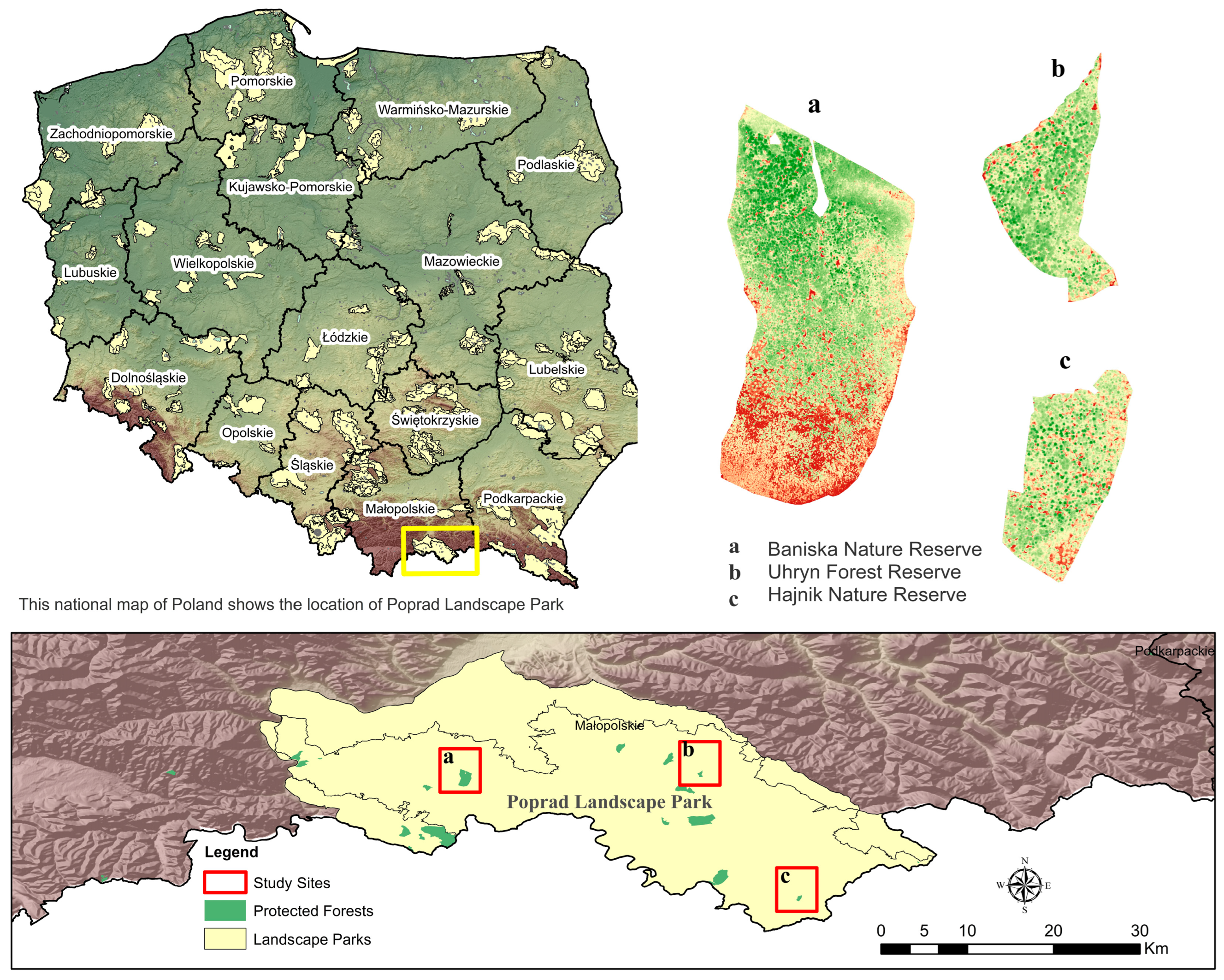
Figure 1. Location of the three forest reserves within the Poprad Landscape Park in the Beskid Sądecki range of the Western Carpathians, Southern Poland.
Remotesensing 18 01045 g001
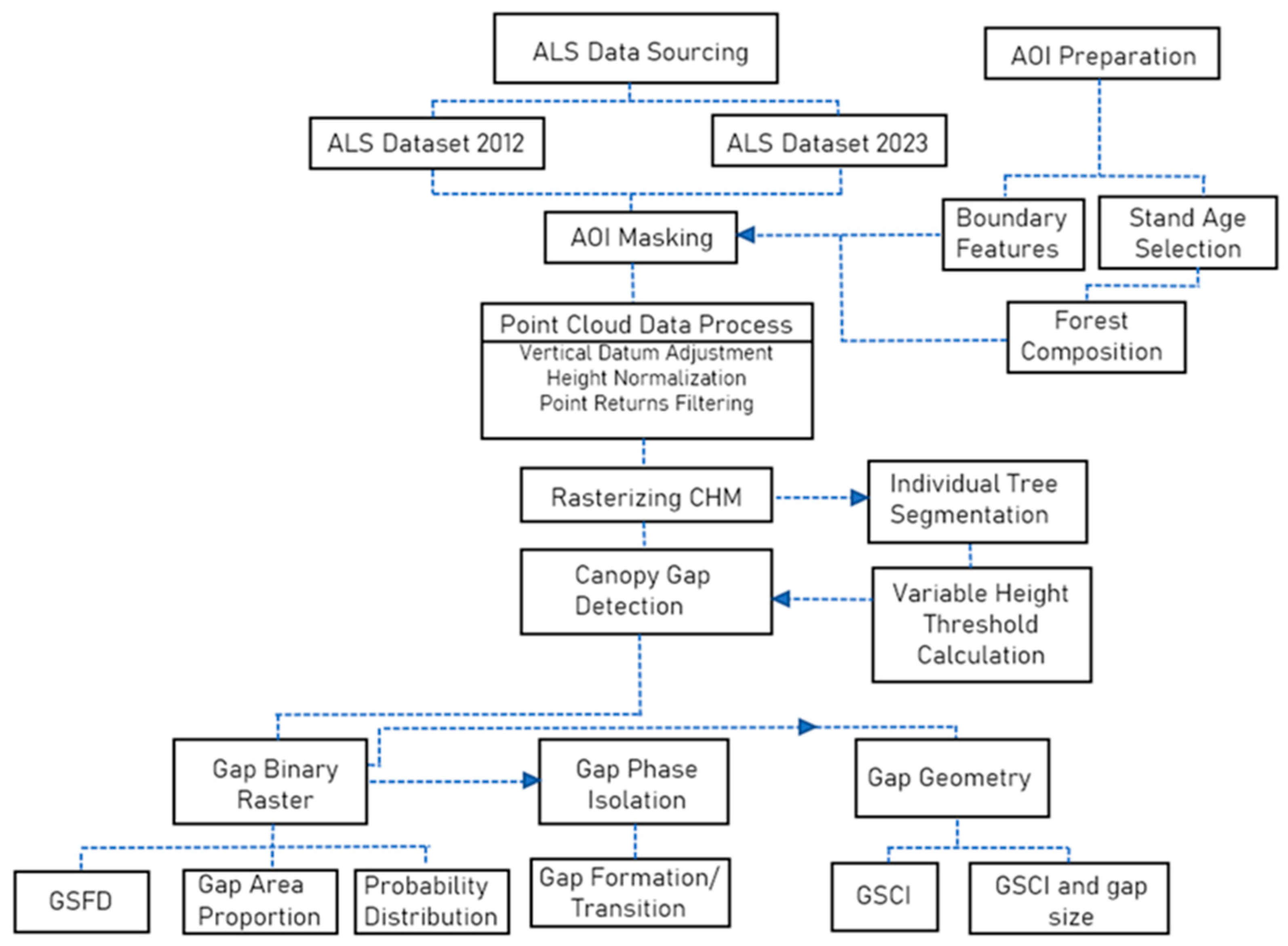
Figure 2. Process flow diagram of the study.
Remotesensing 18 01045 g002
Figure 3. Normalized (gaps-ha) GSFD binned into gap size classes and stratified into (a) protected forest units (sites), and (b) forest types.
Remotesensing 18 01045 g003
Figure 4. Plot of multi-temporal gap metrics gap size and gap shape complexity index for sites (a,c) and forest types (b,d). The horizontal line inside the box represents median values, the × mark represents the mean, and the whiskers represent the data spread. Color-coded compact letter display above the bar shows the results of Kruskal–Wallis + Dunn (BH) test between sites and forest types tested separately for each year (green–2012 and red–2023). Abbreviation below the bar for gap size and GSCI show the result of the Wilcoxon rank-sum test with p-values BH-adjusted for testing the individuals’ significant difference between years (2012 vs. 2023).
Remotesensing 18 01045 g004
Figure 5. Correlation plot of gap size and gap shape for (a) sites and (b) forest types in the years 2012 and 2023 using Kendall’s tau correlation method. The graph shows a moderate positive relationship for gap size and gap shape complexity, indicating greater shape complexity as gap size increases.
Remotesensing 18 01045 g005
Table 1. Profile of the ALS dataset used in the study.
MissionAcquisition YearPoint DensityVertical DatumElevation ReturnsResolution
ISOK 201220124 pts/m2PL-KRON86-NHFirst, Last, Multiple Returns0.5 m
ISOK 202320234 pts/m2PL-EVRF2007-NHFull waveform, Multiple Returns0.25 m
Table 2. Summary table of calculated top height based on 100 highest trees/hectare per stand.
Forest Type100 Ha × Total Area x ¯ Maximum Height
(100 Ha × Total Area of Stand)
Height Threshold
2012202320122023
Pure Stand (Beech)
B1118930.6934.491011
B656631.3833.271011
U233334.436.681112
B1022822.9528.7589
U19424.9329.23810
Mixed Forest—No dominant
B3190137.8233.431211
Mixed Forest (Beech-dominated)
B47231.06341011
B539126.4427.6299
B11343135.7737.571212
B12136630.6932.221011
U3107236.4437.891213
Mixed Forest (Silver Fir-dominated)
H156331.3733.931011
H230731.0234.141011
H380734.7835.891112
U411432.5535.381112
Table 3. Summary table of canopy gap properties for 2012 and 2023 for the site group (protected forest location).
SITEBaniska (88.44 ha)Hajnik (16.77 ha)Uhryn (15.19 ha)
Gap Size ClassFreq. 2012Area (m2)Freq. 2023Area (m2)Freq. 2012Area (m2)Freq. 2023Area (m2)Freq. 2012Area (m2)Freq. 2023Area (m2)
20–50263818714545615818214213022681722732
51–100120873167473825176716108716111111784
101–2006996603955426839111662912856865
201–50032988719557012244118225671204
501–100010666986318 1532
>1000512,154233091109712210
n, total49955,28828030,038915748757975533780402585
n, ha−15.6 3.2 5.4 4.5 3.5 2.6
Mean size, m2111.0 107.0 63.2 106.0 71.3 64.6
Median size, m247.0 49.0 40.0 42.0 52.0 48.0
Gap, %6.33.43.34.82.51.7
Table 4. Summary table of canopy gap properties for 2012 and 2023 for forest types.
Forest TypePure Stand—B (20.88 ha)Mixed Forest ND (19.01 ha)Mixed Forest BD (62.6 ha)Mixed Forest SFD (17.91 ha)
Gap Size ClassFreq. 2012Area (m2)Freq. 2023Area (m2)Freq. 2012Area (m2)Freq. 2023Area (m2)Freq. 2012Area (m2)Freq. 2023Area (m2)Freq. 2012Area (m2)Freq. 2023Area (m2)
20–50351078176095718232170319460251273890611899441393
51–10017116796362719699646906582584106271891181221
101–2005682564481116345564898136520371005121767
201–50013241249411871462288658174859250951386
501–1000 1571 9609886318 1532
>1000 512,15423309110,09712210
n, total58325132213897666634226639048,49824827,6859815,401818509
n, ha−12.8 1.5 5.1 1.8 6.2 4.0 5.5 4.5
Mean size, m256.1 66.8 68.7 66.6 124.0 112.0 65.3 105.0
Median size, m240.0 49.0 44.0 42.5 51.0 48.0 40.5 46.0
Gap, %1.61.03.51.27.84.48.64.8
Summary
Total20122023
No. of gaps643395
Gap area, m264,81640,598
Ha equivalent6.484.06
Overall site area120.4
Table 5. Gap size best fitting probability distribution model selection by maximum likelihood estimation.
GroupYearProbability
Distribution
nαλμσxminKSp_gof
Site
Baniska2012Log-normal499 4.070.9
2023Log-normal280 4.090.92
Hajnik2012Log-normal91 3.80.66
2023Power-law751.97 200.0540.684
Uhryn2012Log-normal53 4.010.69
2023Log-normal40 3.95 0.64
Forest Type
MFBD2012Log-normal390 4.140.94
2023Log-normal248 4.10.94
MFND2012Log-normal97 3.90.72
2023Power-law342.12 200.0690.823
MFSFD2012Log-normal98 3.820.69
2023Power-law811.95 200.0610.431
PSB2012Log-normal58 3.80.61
2023Exponential32 0.01
Table 6. Summary table for gap formation dynamics from 2012 to 2023 showing the percentage of gap formation and closing, and the rate. Gap formation and recovery were categorized into closure, openings (expanding and isolated), and persistent.
CloseExpandingNew OpeningPersistentBalanceStatus
Site Group
Baniska%5395327Recovering
m2 ha−1 yr−1356321
Hajnik%31381219−39Opening
m2 ha−1 yr−11924812
Uhryn%501017230Steady-state
m2 ha−1 yr−115357
Forest type Group
PSB%511114251Recovering
m2 ha−1 yr−110235
MFBD%51105343Recovering
m2 ha−1 yr−1438428
MFND%70571840Recovering
m2 ha−1 yr−125227
MFSFD%32351320−37Opening
m2 ha−1 yr−12022813
Disclaimer/Publisher’s Note: The statements, opinions and data contained in all publications are solely those of the individual author(s) and contributor(s) and not of MDPI and/or the editor(s). MDPI and/or the editor(s) disclaim responsibility for any injury to people or property resulting from any ideas, methods, instructions or products referred to in the content.