Article

Long-Term Sediment Accretion Rates of Floodplains Using Remote Sensing Waterline Extraction Method: A Case Study of Poyang Lake, China


1
School of Geography and Environment, Liaocheng University, Liaocheng 252059, China
2
State Key Laboratory of Lake and Watershed Science for Water Security, Nanjing Institute of Geography & Limnology, Chinese Academy of Sciences, Nanjing 210008, China
*
Author to whom correspondence should be addressed.
Remote Sens. 2026, 18(7), 1044; https://doi.org/10.3390/rs18071044
Submission received: 30 January 2026 / Revised: 25 March 2026 / Accepted: 26 March 2026 / Published: 31 March 2026

Highlights

What are the main findings?
  • The object-based waterline extraction method performs effectively for topographic inversion in floodplain environments, achieving an average area extraction error of 5.55% and mean elevation error below 6.1%.
  • Over the past 40 years, the naturally developed zone of the studied floodplain experienced a mean accretion rate of 3.1 ± 0.7 cm yr−1 (surface elevation change), with mixed CarexT. lutarioriparia vegetation promoting twice the accretion rate of pure Carex communities.
  • Human activities, primarily upstream dam construction and local sand mining, have significantly modulated long-term sediment accretion by reducing sediment supply and removing protective vegetation cover from the floodplain.
What are the implications of the main findings?
  • The remote sensing waterline extraction method proves effective for long-term topographic monitoring in hydrologically dynamic wetlands, with mean elevation errors controllable within 7.0% when sufficient images (≥13) are available. This offers a viable approach for regions lacking continuous field surveys.
  • Findings highlight the critical roles of vegetation zonation in shaping floodplain evolution, supporting targeted strategies for wetland restoration and sediment management under changing anthropogenic pressures.

Abstract

With a typical floodplain in Poyang Lake selected as the study area, this paper employed the remote sensing Waterline Extraction Method (WEM) to invert its topographic changes based on 264 Landsat images from 1987 to 2024. The research systematically revealed the spatiotemporal variations in sediment accretion rates over the past 40 years and their influencing factors. By comparing different WEMs, the object-based method was identified as the most suitable for this study area. Accuracy validation of the topographic inversion showed that when using no fewer than 13 images, the average elevation error rate remained below 7.0%, indicating good reliability. The period from 1987 to 2024 was divided into 15 sub-periods, and digital elevation models of the floodplain were reconstructed for each. Results indicated that: (1) natural floodplain unaffected by sand mining experienced continuous accretion, with an average rate of approximately 3.1 ± 0.7 cm yr−1 (surface elevation change) between 1987 and 2024; (2) in areas impacted by sand mining, the sediment accretion rate after mining (about 1.7 ± 0.8 cm yr−1) was lower than that before mining (about 2.6 ± 2.7 cm yr−1), likely due to the loss of vegetation cover reducing sediment retention capacity; (3) different vegetation types notably influenced accretion rates, with mixed CarexT. lutarioriparia communities showing a consistently higher rate (about 3.5 ± 0.9 cm yr−1) than pure Carex communities (about 1.7 ± 0.7 cm yr−1), primarily attributable to differences in plant morphology, root architecture, and inundation tolerance. Further analysis revealed that riverine sediment supply was the fundamental material source for floodplain accretion. The phased decline in sediment discharge from the Ganjiang and Xiushui rivers since 1996 generally corresponds to the decreasing trend in sediment accretion rates observed after 2004.

1. Introduction

Floodplain wetlands are ecosystems characterized by shallow aquatic environments, primarily distributed in coastal zones, river deltas, estuaries, and lakeshores [1]. The formation of such wetlands is attributed to long-term sediment deposition resulting from weakened hydrodynamic forces. Their hydrological regimes are jointly influenced by tidal fluctuations and seasonal variations in river discharge, exhibiting dynamic patterns of periodic inundation and exposure [2]. This unique hydrological dynamic creates diverse ecological niches, sustaining high species richness and ecosystem complexity [3]. Sediment deposition, as a key process in floodplain development, is regulated by both natural factors (such as precipitation patterns, runoff dynamics, and watershed geology) and human activities (including dam construction, land-use changes, and channel sand mining) [4,5,6]. From an ecological perspective, moderate sediment deposition plays a crucial role in maintaining the spatial structure of floodplain wetlands, promoting vegetation succession, and shaping habitats for organisms [7]. However, excessive deposition may lead to a range of negative ecological effects, including vegetation burial, reduced lake water storage capacity, and water quality deterioration [8]. Therefore, elucidating the spatiotemporal patterns, driving mechanisms, and ecological-environmental responses of sediment deposition rates is of great significance for the integrated management and ecological restoration of floodplain wetlands [9].
The sediment accretion referred to here is defined as the net rate of vertical surface elevation change resulting from mineral sedimentation and organic matter accumulation (e.g., plant roots and detritus), minus erosion and shallow subsidence, typically evaluated on an annual timescale [10]. Methods for measuring accretion rates vary across different spatial and temporal scales. For long-term scales (decades to centuries), paleoenvironmental reconstruction and isotopic dating techniques (such as 14C, 137Cs, and 210Pb) are commonly employed [11]. Over shorter periods, methods such as marker horizon, sedimentation plate, and sedimentation-erosion bars are widely used [12]. Additionally, accretion can be inferred by repeatedly measuring changes in surface elevation, known as the surface-elevation change method [12]. At small spatial scales, this method often relies on ground-based instruments such as levels, total stations, or real-time kinematic (RTK) systems [13], whereas at larger scales, remote sensing technologies such as airborne LiDAR and spaceborne synthetic aperture radar (SAR) are primarily applied [14].
The Waterline Extraction Method (WEM) is a terrain inversion technique for coastal zones and intertidal areas based on multi-temporal remote sensing imagery [15]. This method involves acquiring sequences of satellite or aerial images under varying water level conditions to accurately extract the land-water boundary (i.e., instantaneous waterlines). These extracted waterlines are then matched with corresponding water level elevation data, enabling the reconstruction of regional Digital Elevation Models (DEMs) through spatial interpolation algorithms [16]. The core assumptions of WEM are: (1) the water surface is nearly level across the entire scene (negligible water surface gradient); (2) the effects of wind, seiches, and local hydraulic controls (e.g., disconnections) on the water surface elevation are minimal; and (3) the extracted shoreline represents a single, instantaneous stage corresponding to the recorded water level at the gauge station [15]. Violations of these assumptions can lead to significant errors in the reconstructed DEM.
Due to the highly predictable nature of tidal dynamics and the extensive exposure of intertidal areas during low tide, current research and applications of WEM primarily focus on tidal flat topography inversion [15,17]. For floodplain wetlands characterized by significant water level fluctuations and complex hydrological conditions, the application of WEM is promising but requires careful consideration of its underlying assumptions and potential biases. To the best of our knowledge, dedicated studies validating WEM in such specific settings remain relatively limited. In addition, satellite remote sensing imagery, available since the 1970s, combined with water level monitoring data dating back to the 1950s, provides an opportunity to utilize WEM for reconstructing historical floodplain topography. This approach can reveal long-term variations in sediment accretion rates, serving as an important supplement for studying topographic changes and sediment dynamics in wetlands that lack long-term monitoring systems.
As the largest freshwater lake in China, Poyang Lake serves as a crucial flood-regulation reservoir and an ecologically significant wetland in the Yangtze River Basin. It receives water and sediment inputs from five upstream tributaries (known as the ‘Five Rivers’) and discharges into the Yangtze River, forming a typical river-connected lake system. Sediments carried by the ‘Five Rivers’ deposit along the delta front, gradually forming extensive high-, medium-, and low-elevation floodplains. Influenced by seasonal variations in water inflow from both the Yangtze River and the tributaries, the floodplains of Poyang Lake undergo periodic inundation and exposure, fostering exceptionally rich wetland plant resources and species diversity [18]. Concurrently, sediment accretion on these floodplains alters hydrological conditions, thereby affecting vegetation growth and community succession [19]. In recent years, under the combined influence of natural processes and human activities, the sediment dynamics of Poyang Lake have undergone significant changes [20,21]. For instance, Mei et al. [22] noted that the sediment deposition dynamics in Poyang Lake shifted from being a depositional sink with an annual average accretion of 4.21 million tons during 1960–1999 to an erosional source with an annual average loss of 7.82 million tons during 2000–2012. Gao et al. [20] further highlighted that human activities (particularly the operation of the Three Gorges Project and sand mining in Poyang Lake) have profoundly altered sediment exchange between the Yangtze River and Poyang Lake. Before 2000, the net sediment transport was generally from the Yangtze River into Poyang Lake, but this pattern reversed after 2000, leading to a continuous increase in the proportion of sediment in the Yangtze River’s outflow to the sea originating from Poyang Lake during 2003–2010. This transition marked a shift in the Poyang Lake system from a depositional to an erosional regime.
Despite these advances in understanding the main lake’s sediment budget, research on the sediment accretion processes of Poyang Lake’s floodplains remains relatively limited. Existing studies have provided valuable but fragmented insights. Early investigations using 210Pb dating revealed spatial heterogeneity in accretion rates across different geomorphic units, with rates of 0.80 cm yr−1 for natural levees, 0.36 cm yr−1 for floodplains, and 0.13 cm yr−1 for backswamps [23]. More recent studies have elucidated the coupled relationship between floodplain elevation, inundation duration, and vegetation patterns, demonstrating that hydrological conditions exert a primary control on vegetation distribution, which in turn feeds back on sedimentation processes [19,24]. Furthermore, the role of floodplain vegetation in sediment trapping has been increasingly recognized, with research indicating that densely vegetated areas significantly reduce flow velocity and promote sediment settlement [25]. However, a systematic, long-term (multi-decadal) reconstruction of floodplain vertical accretion rates using remote sensing methods, integrated with analysis of vegetation zonation and anthropogenic disturbances, has been lacking.
To address this research gap, the present study focused on the floodplain wetlands of Poyang Lake, selecting a typical floodplain (Zengmizhou) in its southwestern region as the research object. Zengmizhou, located at the confluence of the Ganjiang and Xiushui rivers, serves as an ideal natural laboratory because it directly receives sediment inputs from these two major rivers and exhibits well-developed vegetation zonation. Based on 264 Landsat remote sensing images from 1987 to 2024, WEM was employed to reconstruct the topography of this region across different periods and analyze sediment accretion characteristics. Firstly, using field-measured topographic data of the floodplain, the accuracy of WEM-derived topography was validated to determine the optimal waterline extraction method and the most suitable number of images for topographic inversion. Secondly, the period from 1987 to 2024 was divided into several intervals, with the topography constructed for each interval. Spatial variations in topographic changes and sediment erosion/deposition patterns over the past 40 years were then analyzed across different zones. Finally, by integrating river sediment discharge data and vegetation characteristics of the floodplain, the main driving factors influencing sediment accretion were investigated.

2. Study Area

This study selects Zengmizhou (29°11′23″–29°12′53″ N, 116°1′36″–116°2′28″ E), a typical floodplain in Poyang Lake, as the research area (Figure 1). Zengmizhou is in the southwestern part of Poyang Lake, north of Wucheng Town at the confluence of the Xiushui River and the north branch of the Ganjiang River. This location was chosen for three key reasons. First, influenced by seasonal water level fluctuations of Poyang Lake, its water level and inundation extent undergo significant dynamic changes throughout the year, providing a wide range of water levels for the WEM. Second, situated at the confluence of Ganjiang and Xiushui, it receives substantial runoff and sediment inputs from both rivers. The Ganjiang River, which has the highest runoff and sediment discharge among the ’Five Rivers’, plays a crucial role in shaping the floodplain. Third, the unique hydrological regime of alternating wet and dry conditions fosters typical wetland vegetation communities across the floodplain.
Since the 2000s, with the rapid urbanization and infrastructure construction in China, sand mining activities have emerged in Poyang Lake and rapidly industrialized, with over 400 sand mining vessels operating during peak periods and an annual extraction volume reaching 240 million tons [26,27]. As one of the main mining areas, the western (SM1) and northern (SM2) sections of Zengmizhou were excavated (Figure 1b). Although the SM1 area has continued to receive sediment deposition after excavation, the intense earlier mining created a distinct topographic depression, resulting in significantly prolonged inundation periods (e.g., up to 280–310 days in 2024). This unique hydrological regime has maintained the area as a bare habitat, contrasting sharply with the well-vegetated ZMZ area, which remained unaffected by sand mining.

3. Materials and Methods

3.1. Data Collection

The remote sensing images used in this study are from the Landsat satellite series, all downloaded from the U.S. Geological Survey (USGS) EarthExplorer platform (https://earthexplorer.usgs.gov/ (accessed on 12 November 2024)). All images used are Landsat Collection 2 Level-2 surface reflectance products, which are already processed for radiometric calibration and atmospheric correction, ensuring inter-sensor comparability [28]. Given that the spatial resolution of Landsat images prior to 1987 is 60 m, this study selected a total of 264 images with a spatial resolution of 30 m from 1987 to 2024 for the floodplain topography reconstruction. Due to the scan line corrector failure on Landsat-7 in 2003, Landsat-5 TM images were used for the period from 1987 to 2011, while Landsat-8/9 OLI images were employed for 2013 to 2024. All images met the quality control criteria of having cloud cover less than 10% and atmospheric visibility above 15 km. Additionally, it was ensured that Zengmizhou was fully visible in the images and in a partially submerged state to facilitate accurate extraction of the land-water boundary.
Based on the Annual Hydrological Report of P. R. China [29], this study utilized daily water level data (Wusong Vertical Datum) from 1987 to 2024 recorded at the Wucheng (Poyang Lake) Hydrological Station (marked by a triangle in Figure 1b) to provide elevation references for each waterline extracted via WEM. To address the temporal matching between remote sensing images and water level data, the following procedure was implemented. First, following the specifications for hydrological data compilation [30], each daily average water level was assigned to 12:00 noon as a representative reference point. Second, for each Landsat image (acquisition time approximately 10:30 AM local time), the instantaneous water level at the acquisition time was estimated using linear interpolation between the water levels of the current day (assigned to 12:00) and the previous day (assigned to 12:00). This approach ensured that the time difference between image acquisition and the interpolated water level reference remained within approximately ±1 h.
Furthermore, to analyze the influence of river sediment discharge on sediment accretion rates of the floodplain, annual sediment discharge data for the Ganjiang River (Wanzhou Station) and the Xiushui River (Wanjiabu Station) from 1985 to 2024 were obtained from the Yangtze River Sediment Bulletin (http://www.cjw.gov.cn/zwzc/zjgb/ (accessed on 5 December 2025)).

3.2. Remote Sensing Image Processing

This study employed four WEMs, i.e., Edge Detection Method (EDM), Supervised Classification Method (SCM), Threshold Segmentation Method (TSM), and Object-Based Method (OBM), to extract waterlines. All processing was performed using ENVI 6.0 and Python (version 3.1.10) with the OpenCV library. For methods requiring image conversion (EDM, TSM), multispectral images were converted to grayscale using a weighted average of the green, red, and near-infrared bands to preserve key spectral information for water-land discrimination [31]. The specific implementation of each method is detailed below.
Edge Detection Method (EDM). The classical Canny edge detection algorithm was employed [32]. (1) Images were read using OpenCV and converted to grayscale, followed by 5 × 5 Gaussian smoothing to suppress noise. (2) Otsu’s algorithm was used for binary segmentation, followed by a 5 × 5 morphological closing to repair edge breaks. (3) Continuous edge was extracted using the Canny algorithm with empirically determined low/high thresholds (50/150). These thresholds were chosen after testing on a subset of images to balance sensitivity and noise reduction. (4) The extracted contours were converted to vector waterline data.
Supervised Classification Method (SCM). The Maximum Likelihood Classification (MLC) method was employed [33]. (1) For each Landsat image, two training sample categories (i.e., water and floodplain) were selected. To ensure representativeness, each category contained no fewer than 10 samples, and the Jeffries-Matusita distance was confirmed to exceed 1.8 (generally considered effectively separable when ≥1.8). (2) The MLC was applied, assuming normal distribution statistics for each class. (3) During post-processing, a majority filter was applied to eliminate the pretzel noise, and the waterline was obtained through edge extraction.
Threshold Segmentation Method (TSM). An improved Modified Normalized Difference Water Index (MNDWI) combined with Otsu’s method was adopted [34,35]. (1) MNDWI was calculated using the green (Band 3 for TM/ETM+ and OLI) and SWIR (Band 5 for TM/ETM+, Band 6 for OLI) bands: MNDWI = (Green − SWIR)/(Green + SWIR). (2) Otsu’s algorithm was applied to the MNDWI image to automatically determine the optimal segmentation threshold, effectively resolving threshold drift issues caused by varying illumination conditions [36]. (3) A binarized mask (1 for waterbodies and 0 for non-waterbodies) was generated, followed by edge extraction to obtain the waterline.
Object-Based Method (OBM). The object-based image analysis method was used [37]. (1) In ENVI’s Feature Extraction module, the optimal segmentation scale was automatically determined using Example-Based Feature Extraction (segmentation scale of 20, merge scale of 80, and texture kernel size of 3), which identifies the optimal segmentation level through inflection point detection on local variance rate-of-change curves. (2) Feature vectors were extracted for each object, including spectral features (mean NDVI calculated by NDVI = (NIR − Red)/(NIR + Red)), spatial features (rectangular fit, boundary index), and texture features (homogeneity). Representative samples of two categories (floodplain and water) were selected. (3) A K-Nearest Neighbor (k = 1, using the nearest single sample to determine the class) classifier was applied for classification. By calculating distances between target objects and training samples, the nearest samples were selected statistically to determine object categories and generate final classification results. Post-classification processing was conducted to extract vector waterlines.

3.3. Field Survey of Topography and Vegetation

To validate the accuracy of topographic inversion, a field survey was conducted on Zengmizhou in December 2024 (dry season with water level of 5.9–7.2 m, Wusong datum, similarly hereinafter). Prior to the survey, 608 validation points were systematically arranged in a 64 m × 64 m grid using the spatial sampling tool in ArcGIS 10.3. Due to water accumulation in some areas during actual sampling, 594 effective measurement points were finally obtained (indicated by yellow dots in Figure 1b).
Elevation measurements were carried out using Real-Time Kinematic (RTK) GPS technology to accurately obtain the latitude, longitude, and elevation values of each point. The RTK system has nominal accuracies of ±1 cm horizontally and ±2 cm vertically. The raw elevations measured were ellipsoidal heights (based on the WGS84 ellipsoid). These were converted to normal heights based on the Wusong elevation datum using transformation parameters derived from known control points and a local quasi-geoid model. The vertical transformation uncertainty is approximately ±3 cm.
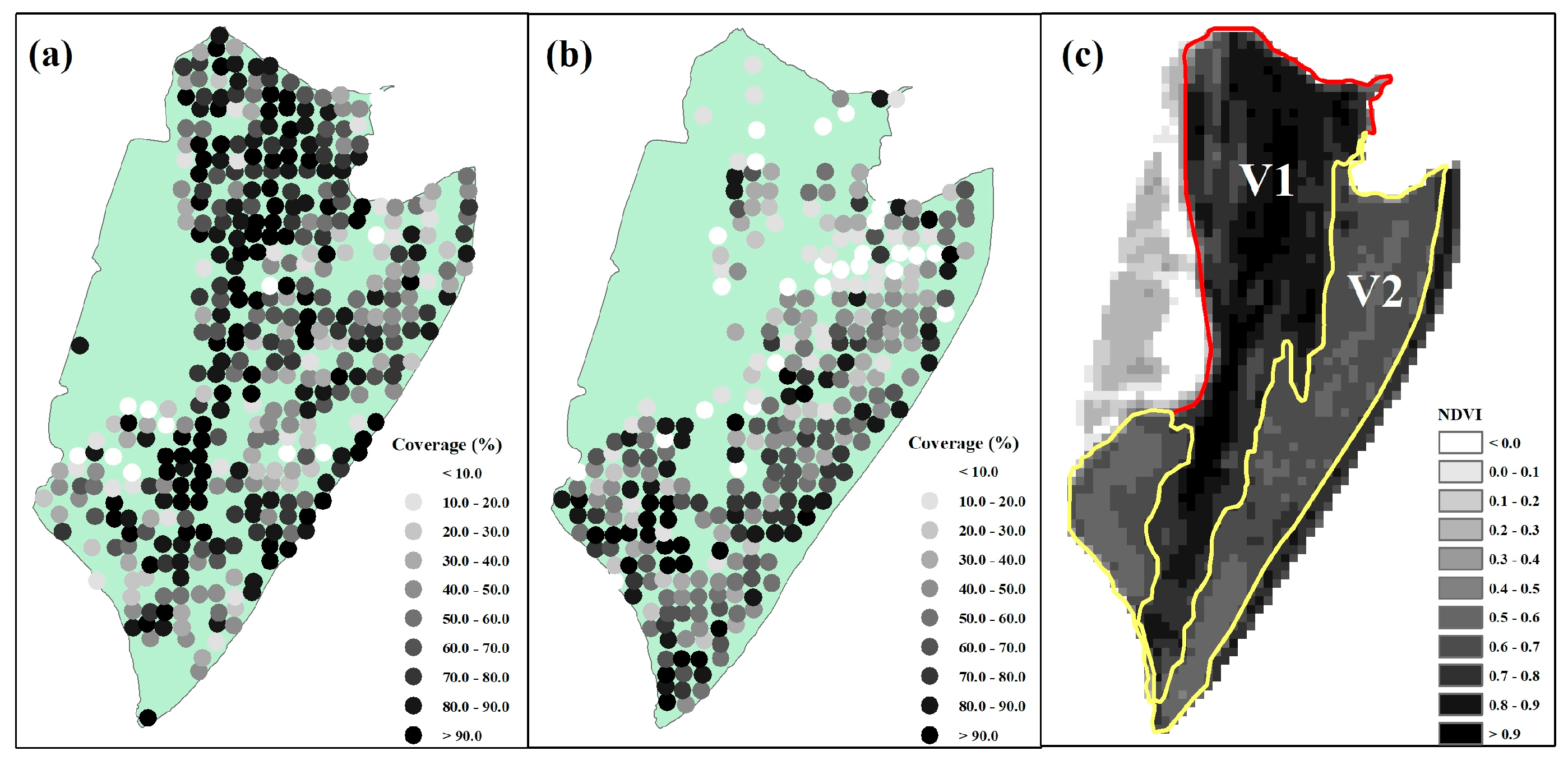
During the topographic survey, vegetation type, height, and coverage data were recorded at each measurement point. This survey confirmed the presence of over ten hygrophytic plant species, with Carex spp. and Triarrhena lutarioriparia being the most widely distributed (Figure 2a,b). Based on the field-observed vegetation composition, a preliminary boundary was manually drawn to separate the area dominated by pure Carex spp. (V1) from the area characterized by a mixed Carex spp. and T. lutarioriparia community (V2) (Figure 2c). This field-based delineation was used for subsequent sampling stratification and was later validated using NDVI analysis (Section 4.3).
Global Moran’s I index was calculated to assess potential spatial autocorrelation among the elevation values of the 594 effective validation points in ArcGIS. The resulting Moran’s I was 0.73 (z-score = 64.98, p < 0.001), confirming statistically significant positive spatial autocorrelation. To address this spatial autocorrelation and obtain more robust accuracy estimates, a stratified random sampling strategy was applied to create a spatially thinned validation subset. The study area was stratified based on vegetation zones (V1, V2) and elevation classes (low: <12 m, medium: 12–14 m, high: >14 m), resulting in six strata. From each stratum, 30% of the original validation points were randomly selected, yielding a reduced validation dataset of 179 points. A spatial blocking cross-validation procedure was then performed, with the study area divided into 8 spatial blocks, and an 8-fold cross-validation was conducted by iteratively holding out one entire block for validation while training on the remaining seven.

3.4. Accuracy Validation of WEM and Topographic Inversion

Based on 25 remote sensing images acquired from 2023 to 2024, waterlines were extracted using the four methods. Ten image quantity gradients (7, 9, 11, 13, 15, 17, 19, 21, 23, and 25 images) were set, with the image composition and corresponding water level information for each gradient detailed in Table 1. Topographic models of the floodplain were subsequently constructed. Accuracy validation was conducted based on two aspects: the consistency of area and the accuracy of terrain elevation.
First, the relative error ΔS between the predicted area (Sp) from the extracted waterline and the actual area (Sm) from the RTK-measured DEM for the corresponding water level was calculated:
Δ S = S m S p / S m × 100 %
Given that the measured elevation range of Zengmizhou was 8.0 m to 16.5 m, only images corresponding to water levels between 9.0 and 15.5 m were used for validation to ensure reliability.
Second, the Jaccard coefficient (J) and Kappa coefficient (κ) were employed to evaluate spatial agreement. The Jaccard coefficient is defined as the ratio of the intersection to the union of the area of the extracted region (A) and the actual region (B) [38]:
J = A B A B
The Kappa coefficient is a statistical measure that quantifies the level of agreement between two classifications while accounting for the agreement that could be expected by chance alone [39] and is calculated as:
κ = P 0     P e 1     P e
where P0 is the observed agreement and Pe is the expected agreement based on chance, calculated from the marginal sums of a confusion matrix. It ranges from −1 to +1, with values > 0.8 indicating almost perfect agreement. To optimize computational efficiency, three representative water levels, i.e., low (H = 9.27 m), medium (H = 12.86 m), and high (H = 15.40 m), were selected to calculate κ and Overall Accuracy (OA, representing the proportion of correctly classified pixels).
Subsequently, based on the extracted waterlines and their corresponding water levels, the ordinary Kriging interpolation (using a spherical variogram model with default parameters optimized by the software based on the input point data) was used in ArcGIS to reconstruct the floodplain’s topography. To account for spatial autocorrelation in validation points, the spatially thinned validation dataset (179) derived from stratified random sampling was used for primary accuracy assessment. The predicted elevation (Ei_p) was obtained at these validation points and compared with the RTK-measured elevation (Ei_m) to compute the mean absolute error:
Δ E = 1 / 179 i = 1 179 E i = 1 / 179 i = 1 179 E i _ m E i _ p / E i _ m × 100 %
The 8-fold spatial block cross-validation yielded a range of ΔE values (minimum to maximum across folds), which is reported alongside the primary ΔE to provide a conservative uncertainty estimate that accounts for spatial dependence.
Due to the inter-annual variability in the availability of suitable remote sensing images (ranging from 2 to 16 scenes per year), the entire study period (1987–2024) was divided into several sub-periods. For each sub-period, a DEM was reconstructed and the mean elevation of the target zones (ZMZ, SM1, V1, V2) was calculated. To estimate the long-term sediment accretion rate, a linear regression was fitted to the time series of these mean elevation values. The slope of the regression line (k, in m day−1) represents the daily accretion rate, which was then converted to an annual rate (cm yr−1) by multiplying by 365.25 × 100. The standard error of the regression slope was used to provide an uncertainty estimate for each accretion rate. To complement the parametric linear regression and provide a more robust assessment of trend significance that is less sensitive to outliers and does not assume normality, the non-parametric Mann–Kendall (M-K) trend test and Sen’s slope estimator were also applied. In addition, a two-sample t-test was used to compare accretion rates between different zones and periods, with a significance level of p < 0.05.

4. Results

4.1. Accuracy of Topographic Inversion

The errors in floodplain area extracted by the four WEMs are shown in Table 1. The EDM had the highest mean relative error (ΔS) of 29.67%, representing the poorest performance among the four methods, and the ΔSi under certain water levels even exceeded 80%. The SCM yielded a ΔS of 15.29%, and except for the high-water level (H = 15.40 m) where ΔSi reached 60.70%, the ΔSi values were all below 25%. In comparison, the TSM (ΔS = 6.27%) and OBM (ΔS = 5.55%) performed better. Except for the water level H = 15.40 m, their ΔSi values all remained within 10.0%. Moreover, at this water level, the OBM (ΔSi = 32.61%) outperformed the TSM (ΔSi = 54.50%) in extracting the floodplain area. The Jaccard similarity coefficient (J) for the different methods showed that the EDM had the lowest mean J value (0.782), followed by TSM (0.848), SCM (0.853), and OBM (0.861). In terms of the Kappa coefficient (κ) and Overall Accuracy (OA), the EDM had the lowest values (κ = 0.677, OA = 0.864), while the OBM achieved the best performance (κ = 0.876, OA = 0.953).
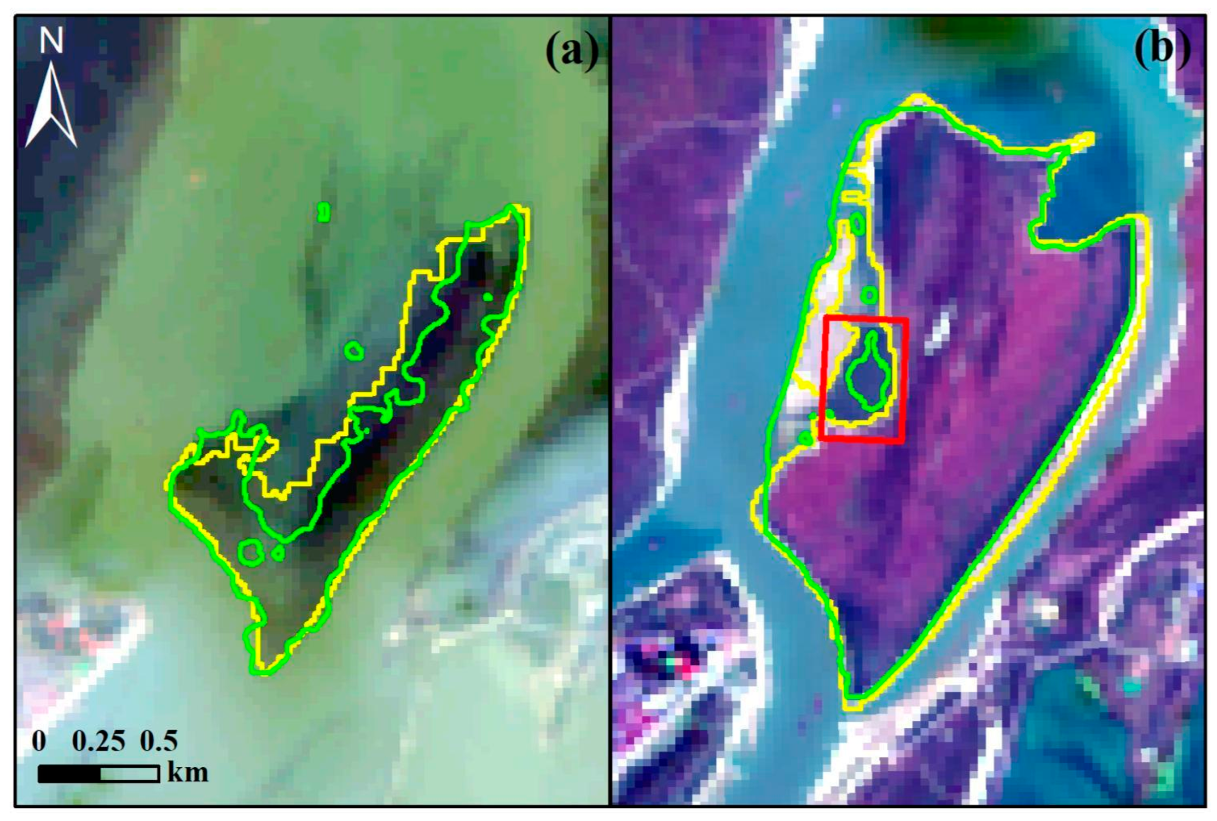
Accuracy analysis indicated that four WEMs performed poorly under high water level conditions. This was primarily due to the partial or complete submergence of wetland vegetation, which significantly altered the surface reflectance of water bodies [40], thereby increasing errors in water-land boundary extraction (Figure 3a). For instance, at a water level of H = 15.40 m, the ΔSi values for EDM, TSM, SCM, and OBM were 70.98%, 54.50%, 60.70%, and 32.61%, respectively, with J values of 0.516, 0.555, 0.596, and 0.686, and κ values of 0.600, 0.675, 0.747, and 0.880. In comparison, the OBM, which integrates texture features and employs multi-scale segmentation, demonstrated significantly superior accuracy in waterline extraction over the other methods. However, limited by the resolution of remote sensing imagery, the mixed-pixel effect caused by emergent vegetation remains a major factor influencing extraction accuracy.
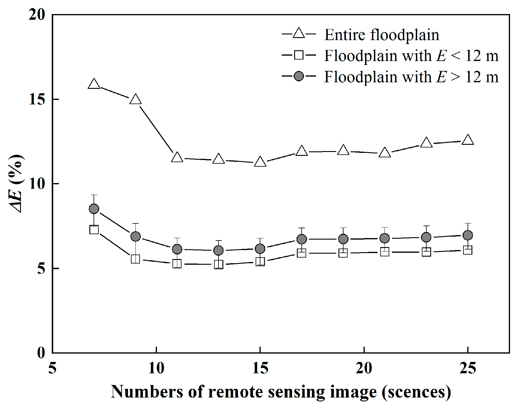
Given the excellent performance of the OBM in waterline extraction, it was adopted in this study to reconstruct the floodplain topography. Figure 4 shows the mean error rate (ΔE) for the OBM across the 10 image quantity gradients, calculated using the 179 spatially thinned validation dataset. As illustrated, ΔE ranged from 6.1% to 8.5%, showing an overall decreasing trend with increasing image quantity. Specifically, when the image count increased from 7 to 13, ΔE decreased significantly from 8.5% to 6.1%. With more than 13 images, ΔE stabilized with a slight upward trend (e.g., 6.7% with 17 images, 7.0% with 25 images). This slight increase was due to the limited availability of high-water-level images, and the additional images were predominantly from low water levels (Table 1). When using WEM to construct floodplain topography, the inversion errors for low-elevation (E < 12 m) areas were typically higher than those for high-elevation (E > 12 m) areas. As shown in Figure 3b, for low-elevation areas like SM1, local depressions can become hydraulically disconnected from the main channel during water recession, forming isolated water bodies. This leads to a discrepancy between the extracted waterline and the true topographic contour (indicated by the red box in Figure 3b), increasing the inversion error in these low areas and contributing to the overall error when more low-water-level images are included.
It is important to note that the vertical reconstruction error (ΔE) represents a relative error percentage. For the floodplain elevation range of approximately 8.0–16.5 m, ΔE of 6.1–7.0% (when using ≥13 images) corresponds to an absolute elevation uncertainty of approximately 0.5–0.8 m per DEM. This uncertainty propagates into the estimation of accretion rates, which are derived from elevation differences between DEMs from different periods. Consequently, the absolute accretion rate values reported in this study should be interpreted with this uncertainty in mind. However, as demonstrated in the following sections (Section 4.3), the relative differences in accretion rates between zones (e.g., vegetated vs. non-vegetated, different vegetation communities) and the temporal trends revealed by multiple independent sub-periods provide robust insights that are less sensitive to absolute calibration errors.

4.2. Area-Elevation Relationship of the Floodplain

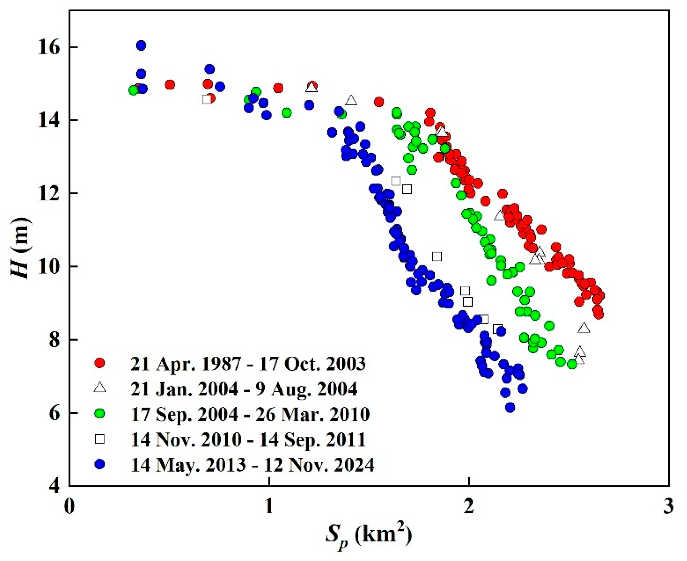
Waterlines were extracted from 264 remote sensing images spanning 1987 to 2024 using the OBM. The relationship between the area enclosed by each waterline and its corresponding water level elevation is shown in Figure 5. Influenced by human sand mining activities, the data points cluster into three distinct groups, reflecting three evolutionary phases of the floodplain’s topography. Based on remote sensing image interpretation, sand mining activities on Zengmizhou occurred during two periods: January to August 2004 (excavation of the SM1 area, represented by triangles in Figure 5) and November 2010 to September 2011 (excavation of the SM2 area, squares). Accordingly, the topographic evolution of the floodplain can be divided into five periods: two excavation periods and three naturally stable periods (April 1987–October 2003, red dots; September 2004–March 2010, green dots; and from May 2013 to present, blue dots). Sand mining led to a significant reduction in floodplain area, causing the area-elevation curve to shift downward after each excavation period. In contrast, during the stable periods, the area-elevation relationships remained relatively consistent.
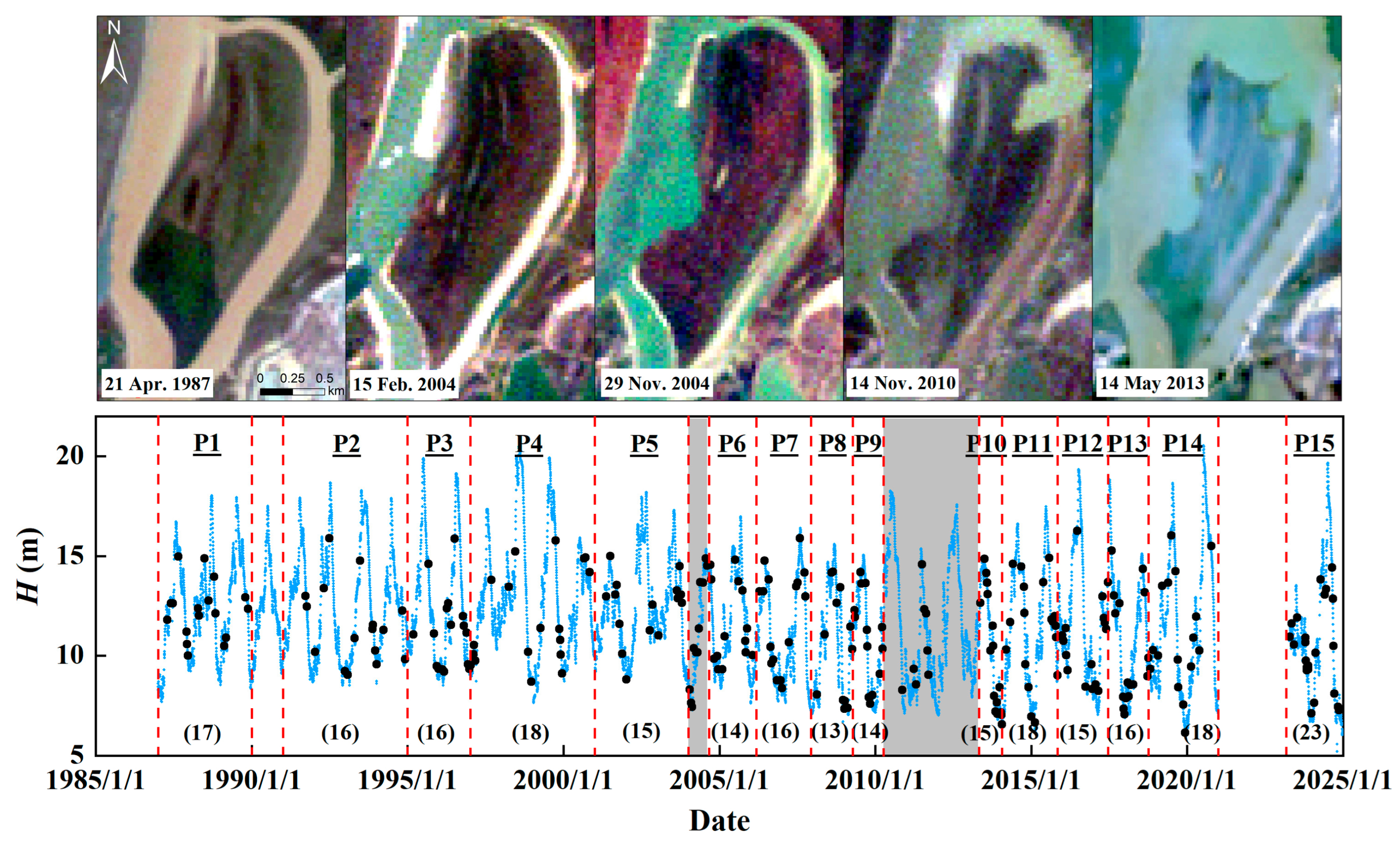
In the present study, the entire period (1987–2024) was divided into several sub-periods based on two criteria: (1) major hydrological events and known periods of human activity (i.e., the two sand mining phases); (2) the need to ensure a sufficient number of images (≥13) in each sub-period to maintain inversion accuracy, as determined in Section 4.1. It should be noted that the topography of the floodplain undergoes certain changes after each flood season, and longer time spans may introduce significant topographic variation errors. To balance the trade-off between time span and image quantity, the three stable periods were further divided into 15 sub-periods with the number of images used for each shown in Figure 6. The floodplain’s topography was reconstructed for each sub-period, enabling a comparative analysis of sediment accretion rates over the past 40 years. The two excavation periods were excluded from topographic inversion due to rapid terrain changes primarily driven by human activities.

4.3. Characteristics of Sediment Accretion in the Floodplain

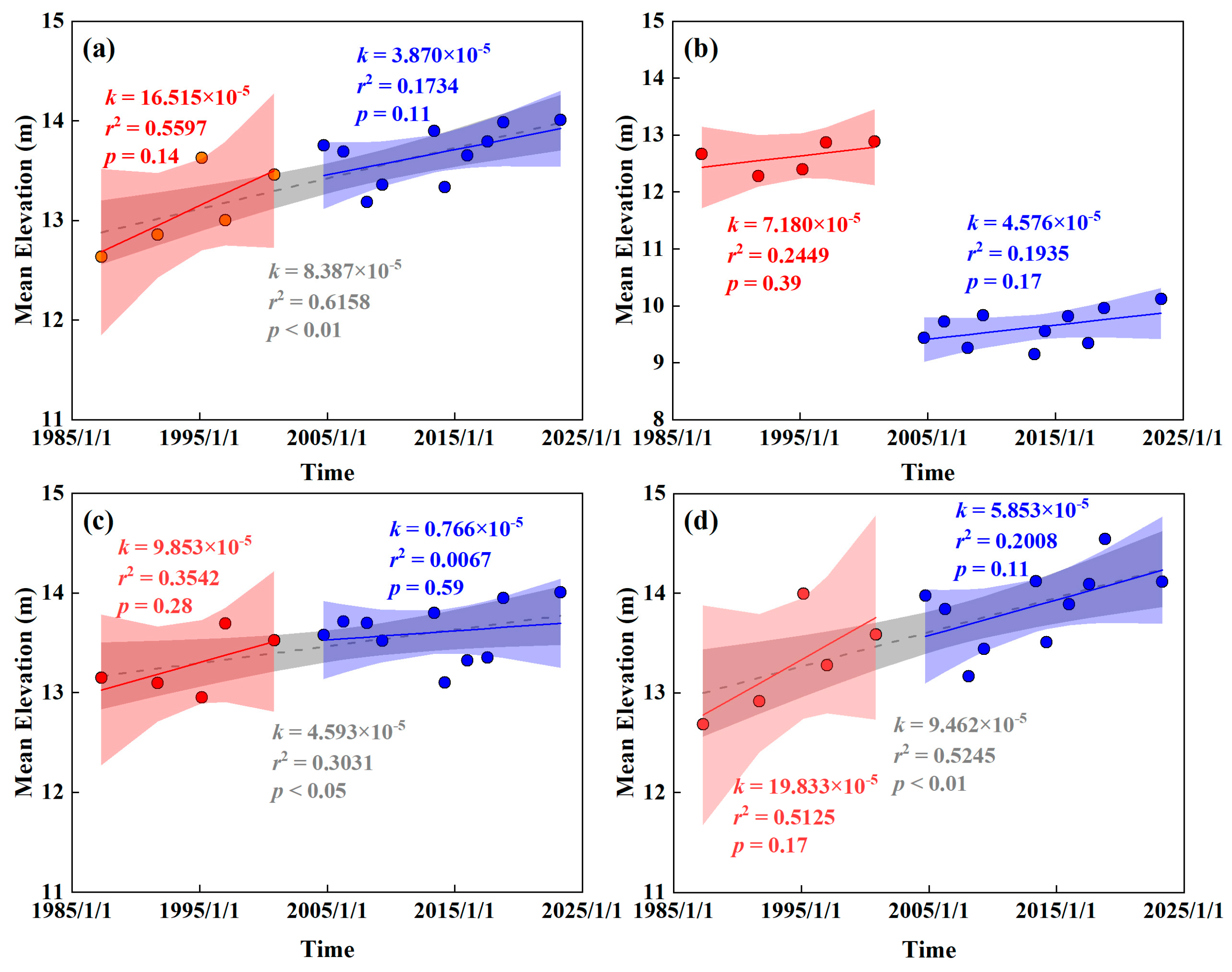
Linear fitting of the time series of mean elevation for the ZMZ area (unaffected by sand mining activities) from 1987 to 2024 (Figure 7a) yielded a slope corresponding to an annual accretion rate of 3.1 ± 0.7 cm yr−1 (r2 = 0.62, p < 0.01). To more robustly assess this long-term trend, a non-parametric M-K trend test and Sen’s slope estimator were applied. The results showed a M-K statistic (Z) of 3.07 (p < 0.01) for the ZMZ elevation time series, with a Sen’s slope estimate of 3.3 cm yr−1, which is highly consistent with the linear regression result and confirms the significance of the long-term net accretion trend in this area. When the entire period was segmented at the first sand mining period (January–August 2004), the pre-mining (January 1987–December 2003) rate was 6.0 ± 3.1 cm yr−1 (r2 = 0.56, p = 0.14), while the post-mining (September 2004–December 2024) rate was lower at 1.4 ± 0.7 cm yr−1 (r2 = 0.17, p = 0.11). Although the post-mining rate was substantially reduced, a t-test comparing the pre- and post-mining regression slopes did not reach statistical significance (t = 1.46, p = 0.17), likely due to the limited number of sub-periods available for the segmented analysis (5 for pre-mining, 10 for post-mining).
For the SM1 area (Figure 7b), the pre-mining accretion rate was 2.6 ± 2.7 cm yr−1 (r2 = 0.24, p = 0.39). The post-mining rate decreased to 1.7 ± 0.8 cm yr−1 (r2 = 0.19, p = 0.17). The M-K test revealed that the increasing trends in SM1 elevation were not significant for either the pre-mining (Z = 1.22, p = 0.22) or post-mining (Z = 1.43, p = 0.15) periods. However, the Sen’s slope estimates (decreasing from 2.9 cm yr−1 to 1.6 cm yr−1) aligned with the linear regression results. This reduction may be attributed to the low-lying topography formed after sand mining in the SM1 area and the absence of vegetation cover post-2004, which likely weakened its sediment-trapping capacity compared to the earlier vegetated phase.
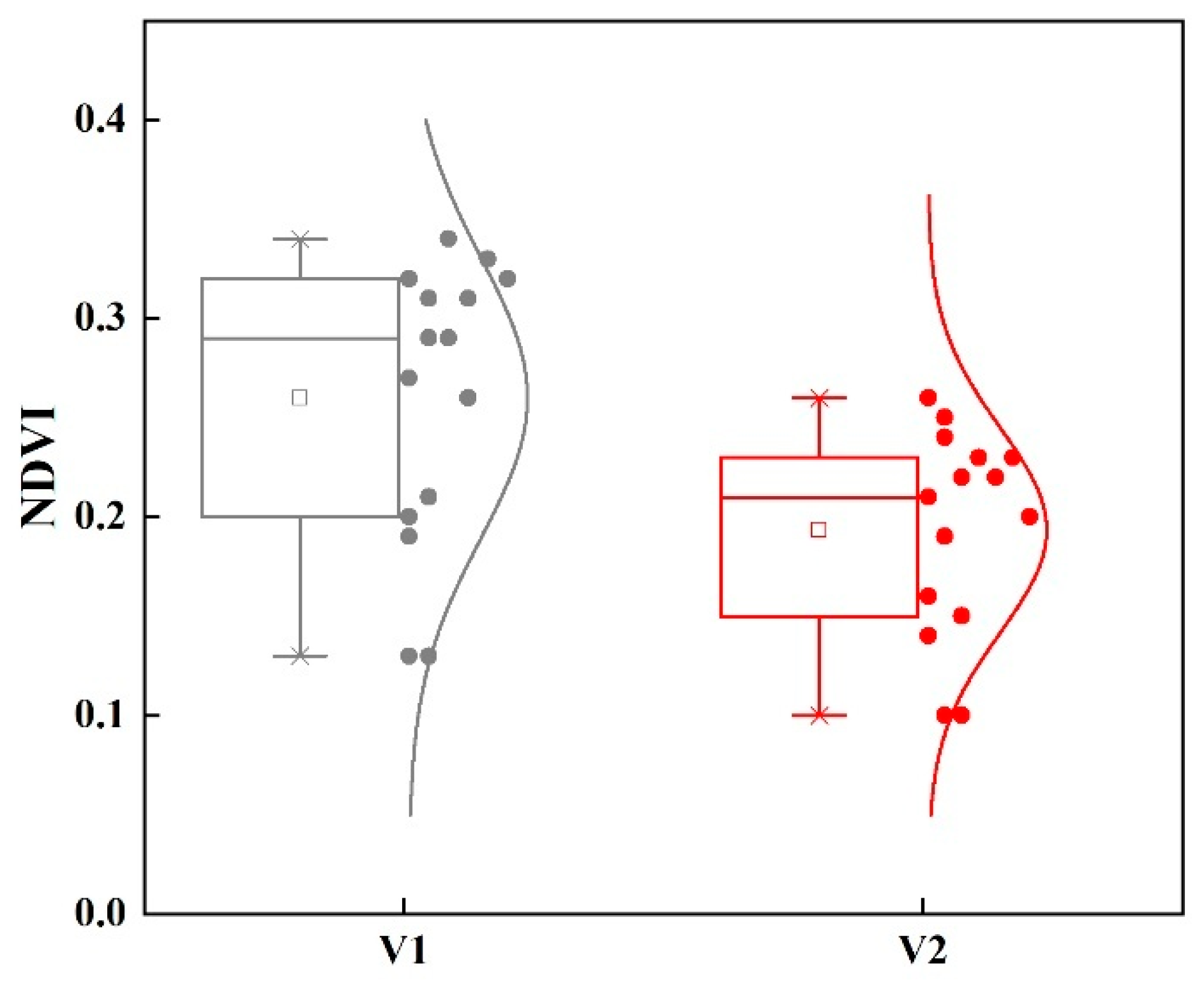
The zonal distribution of vegetation along the elevation gradient within the floodplain provides an opportunity to investigate differences in sediment accretion rates across different vegetation types. Due to the phenological differences between Carex spp. (two growing seasons, with its second growing season beginning after the flood season and reaching the maximum coverage in October) and T. lutarioriparia (budding in March, reaching their maximum coverage in late September and then gradually withering and turning yellow in late autumn), their spectral signatures differ markedly in post-recession autumn (November) [41]. This allows for their discrimination using Normalized Difference Vegetation Index (NDVI) around November each year. The delineation of vegetation zones was performed using a two-step approach to ensure robustness. First, as mentioned in Section 3.3, a preliminary boundary was manually drawn to separate the area dominated by pure Carex spp. (V1) from the area characterized by a mixed Carex–T. lutarioriparia community (V2). Second, to quantitatively validate this field-based division and to enable historical analysis, the NDVI from a cloud-free Landsat image acquired on 12 November 2024 (post-recession autumn) was calculated, and the NDVI values in V1 and V2 were significantly different (p < 0.05) (Figure 2).
To verify whether this functional zonation has remained stable over the past 40 years, the mean NDVI for each zone from one cloud-free autumn image in each of the 15 historical sub-periods was calculated. As shown in Figure 8, the NDVI in V1 was consistently and significantly higher than in V2 across all sub-periods (p < 0.05). This result confirms that, despite inter-annual variability in absolute NDVI values driven by climatic and hydrological fluctuations, the distinct spectral difference between the two vegetation communities has persisted. Based on this, trend analysis of elevation evolution in the V1 and V2 zones was conducted to explore the influence of vegetation type on accretion rates. For the V1 (Carex-dominated) zone (Figure 7c), the accretion rate over the entire period was 1.7 ± 0.7 cm yr−1 (r2 = 0.30, p < 0.05). The M-K test confirmed a significant increasing trend (Z = 1.88, p < 0.05), with a Sen’s slope of 1.9 cm yr−1. For the V2 (mixed community) zone (Figure 7d), the rate was significantly higher at 3.5 ± 0.9 cm yr−1 (r2 = 0.53, p < 0.01), and both the M-K test (Z = 2.67, p < 0.01) and Sen’s slope (3.9 cm yr−1) corroborated the significant upward trend. Although a t-test comparing the two regression slopes revealed no statistical significance (t = 1.53, p = 0.14), the V2 zone exhibited a consistently higher accretion rate throughout the entire 40-year study period. Additionally, segmented linear fitting and M-K tests revealed that the slopes for both zones were higher before sand mining than after, suggesting that sediment accretion rates in both V1 and V2 were greater before 2004 than after.

5. Discussion

5.1. Factors Affecting Sediment Accretion Rate

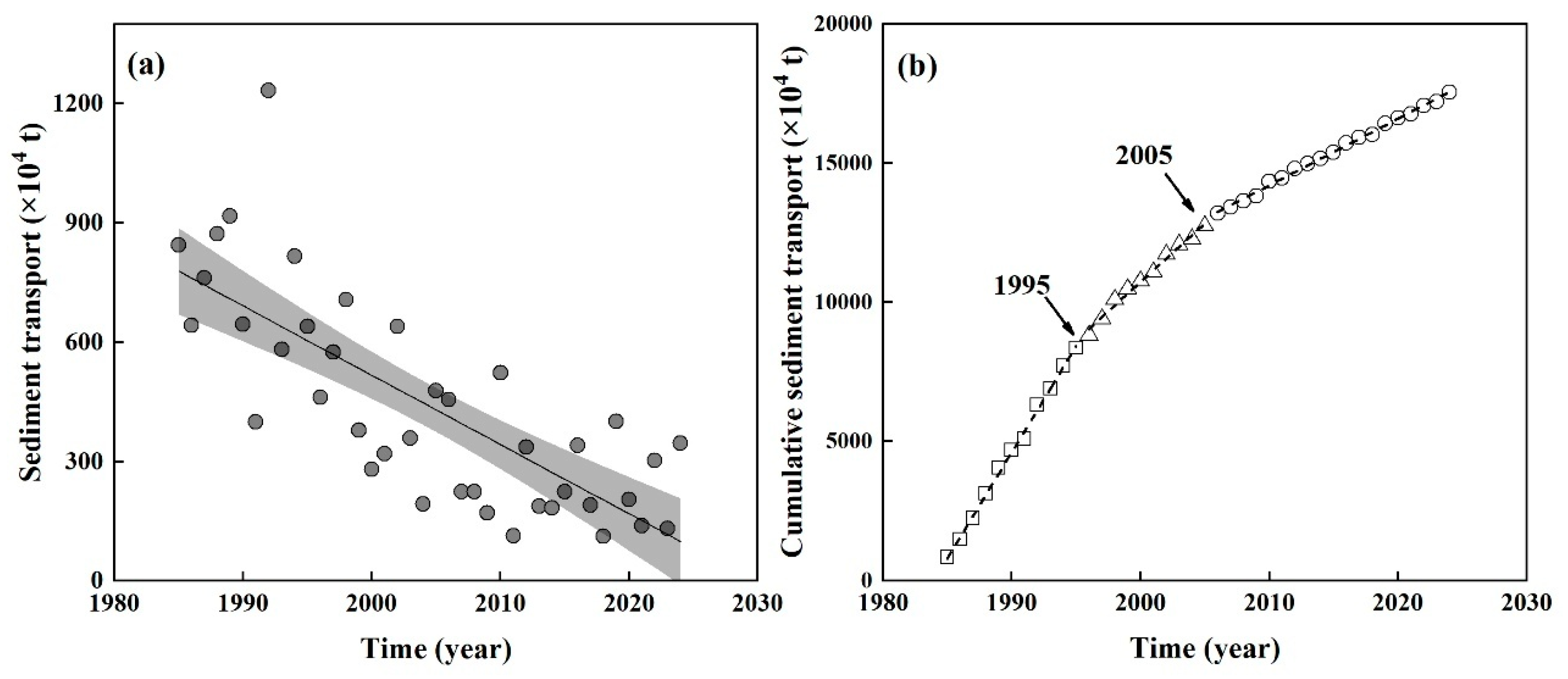
River sediment transport serves as the primary material source for sediment deposition on the floodplain. From 1985 to 2024, the average annual sediment discharge of Ganjiang (Wan’an Station) and Xiushui (Wanjiapu Station) was 438.9 × 10⁴ t, with Ganjiang accounting for 93.1% (408.7 × 10⁴ t). The total sediment discharge showed a significant phased declining trend (Figure 9a), which can be divided into three stages, i.e., 1985–1996 (average 734.6 × 10⁴ t yr−1), 1996–2005 (439.2 × 10⁴ t yr−1), and 2005–2024 (253.1 × 10⁴ t yr−1), based on the cumulative sediment discharge time series (Figure 9b). Liu et al. [42] attributed this reduction to soil and water conservation efforts and the construction of reservoirs, particularly the impoundment of the Wan’an Reservoir on the Ganjiang River after 1996. This phased decline in sediment supply corresponds well with the decreasing trend in accretion rates observed on the floodplain (Figure 7). The high sediment discharge during 1985–1996 drove faster accretion rates in ZMZ (6.0 cm yr−1), SM1 (2.6 cm yr−1), and both vegetation zones before 2004. The subsequent decline in sediment load aligns with the post-2004 reduction in accretion rates across all zones. This correspondence strongly supports the idea that riverine sediment supply is the fundamental control on long-term floodplain accretion rates in this system [22].
As a key component of the floodplain ecosystems, hygrophytic vegetation significantly influences sediment deposition processes. In the present study, sediment accretion rates in vegetated areas were higher than in non-vegetated areas, and the mixed Carex–T. lutarioriparia community (V2) exhibited a higher deposition rate than that of the pure Carex community (V1). This was consistent with field observations and flume experiments showing that vegetation promotes sediment settlement by reducing flow velocity and increasing bed roughness [43,44]. The difference between V1 and V2 can be explained by several mechanisms related to plant traits. First, T. lutarioriparia is a tall, robust herb with rigid, erect stems that can remain standing even when submerged, creating greater drag and a more effective baffle for sediment-laden water compared with the prostrate, more flexible leaves of Carex [45]. Secondly, T. lutarioriparia develops a thicker and deeper rhizome and root system [46], which not only stabilizes a larger volume of captured sediment but also contributes more to belowground organic matter accumulation [47]. Thirdly, its distribution at relatively higher elevations results in shorter inundation periods, favoring greater litter accumulation and in situ organic matter production, which adds to the vertical accretion [48]. In contrast, the rapid decomposition of Carex aboveground biomass upon submergence [41] reduces its capacity to trap sediment during the main flood season. This study demonstrates a clear correlation between vegetation type and accretion rate, but distinguishing between the direct physical effects of the plants on sediment trapping and the indirect effects through organic matter accumulation requires further, process-based research.

5.2. Comparison with Existing Studies and Synthesis of Regional Sediment Dynamics

Our calculated accretion rates for the ZMZ area (3.1 cm yr−1 over 1987–2024) appear to contrast with studies that have documented a shift towards net erosion in the main lake area since the 2000s [20,21,22]. For instance, Zhang et al. [49] reported an average annual lakebed erosion rate of 14.4 cm yr−1 between 2000 and 2010 using a similar waterline method. This apparent discrepancy is not contradictory but rather highlights the distinct geomorphic processes operating in different parts of the lake system. The main lake channel and deep-water areas are subject to stronger scouring flows, exacerbated by the altered river-lake interaction and reduced sediment supply from the Yangtze River, leading to net erosion [20]. In contrast, our study area (Zengmizhou) is a marginal floodplain at the active confluence of two major rivers, which functions as a terminal sink for the remaining sediment load. It continues to experience net vertical accretion even as the overall sediment budget of the lake has become negative.
Furthermore, our rates are substantially higher than those reported in Han and Zhu [23], which revealed sedimentation rates of 0.80 cm yr−1 for natural levees, 0.36 cm yr−1 for floodplains, and 0.13 cm yr−1 for backswamps using 210Pb dating. The order-of-magnitude difference can be attributed to several factors. First, the two studies address fundamentally different temporal scales and incorporate different processes. The 210Pb-derived rates represent long-term (centennial-scale) net accumulation that includes compaction, decomposition, and shallow subsidence over the entire sediment column [50]. In contrast, our WEM-derived rates represent decadal-scale surface elevation changes that are closer to ‘raw’ accretion before significant compaction. The difference between 0.36 cm yr−1 (compacted, centennial average) and 3.1 cm yr−1 (near-surface, decadal rate) is consistent with compaction ratios reported for organic-rich wetland soils, where surface sediments can have 5–10 times higher porosity and lower bulk density than deeper, compacted sediments [51]. Second, the geomorphic context differs. Han and Zhu’s floodplain sampling sites were in different, potentially more distal or lower-energy depositional environments, whereas our site at the delta front receives coarser sediment and experiences higher energy flows, naturally leading to higher accretion rates [52].
Regarding the influence of vegetation, our finding that mixed Carex–T. lutarioriparia communities trap more sediment than pure Carex communities corroborates findings from other Yangtze River-connected lakes. In Dongting Lake, Zhang et al. [44] conducted field flume experiments and found that taller, more robust vegetation (Phragmites australis) created greater flow resistance and trapped significantly more sediment than shorter, flexible vegetation (Carex spp.). Our study confirms this biophysical mechanism at a landscape scale over several decades, providing strong evidence for the functional role of different vegetation types in shaping floodplain topography. This consistency across different lakes and methodologies reinforces the general understanding that plant morphology is a key control on sediment trapping efficiency in wetland environments [53,54]. However, our results differ from some modeling studies that suggest vegetation might only enhance sedimentation during moderate flood events and could be less effective during extreme floods when flow velocities are high enough to cause resuspension [55]. Our long-term average data likely integrate across these event-scale variations, showing a net positive effect of vegetation over multi-decadal periods. This highlights the importance of combining long-term analyses with mechanistic field and modeling studies to fully understand vegetation-sedimentation feedbacks across different temporal scales.
In summary, by quantifying long-term floodplain accretion rates and linking them to both upstream sediment supply and local vegetation, this study provides a more complete and nuanced understanding of the sedimentary dynamics in large floodplain lake systems. It demonstrates that while the system as a whole may be losing sediment, its ecologically vital floodplain margins can continue to build elevation—a process that is significantly modulated by the type of vegetation they support and one that operates at rates substantially higher than long-term compacted averages.

5.3. Limitations and Future Research

While this study provides valuable insights into long-term floodplain evolution, several methodological limitations and knowledge gaps must be acknowledged to contextualize our findings and guide future research directions.
1. Inherent limitations and error sources of the WEM. The core methodology of this study, WEM, has inherent biases when applied to hydrologically complex floodplains that cannot be eliminated. First, as detailed in Section 4.1, under high water level conditions, the partial or complete submergence of vegetation blurs the spectral distinction between water and land, leading to a sharp decline in extraction accuracy. Second, during water recession, low-lying areas (e.g., the SM1 zone) can become hydraulically disconnected from the main channel, forming isolated water bodies (Figure 3b). In addition, the water level from Wucheng station is assumed to be representative of the entire study area, but wind setup, local precipitation, or complex topography could create water surface gradients within the floodplain. These directly violate a fundamental assumption of WEM—that the water surface is continuous and its elevation is uniform and represented by the gauge station [15]. Future research should explore strategies to mitigate this bias, such as using higher-resolution imagery to better identify and mask these disconnected water bodies, or developing post-processing algorithms informed by hydrodynamic models to correct for their influence.
2. Uncertainty in reconstructing historical vegetation distribution. The method used to delineate historical vegetation zones has inherent uncertainties. While we validated the contemporary zonation with field data and confirmed its spectral stability over time using multi-temporal NDVI analysis (Figure 8), this approach assumes that the spatial boundaries between the V1 and V2 zones have remained fixed over the 40-year study period. This assumption may not fully account for potential decadal-scale shifts in community composition or boundary migration driven by climate variability, hydrological changes, or ecological succession. Therefore, our conclusion that the accretion rate difference is directly and consistently attributable to the two vegetation types over the entire study period, while plausible, must be treated with caution. Future research must employ more robust methods to validate and reconstruct historical vegetation cover.
3. The unresolved composition of accretion. The ‘accretion rate’ reported in this study represents the net vertical elevation change, which is the integrated result of three processes: mineral sediment deposition, in situ organic matter accumulation (from roots and litter), and shallow subsidence/decomposition. Our analysis cannot distinguish the relative contributions of these components. This is a crucial distinction, particularly for the V2 zone, where the higher accretion rate could be due to more efficient trapping of mineral sediment by the tall T. lutarioriparia stems, greater production and preservation of organic matter from its dense root system and litter, or a combination of both [48]. Future research should combine the use of surface elevation tables, marker horizons, and sediment cores analyzed for bulk density and organic matter content to quantitatively partition the contributions of mineral and organic matter to total accretion under different vegetation communities.

6. Conclusions

This study selected a typical floodplain (Zengmizhou) in Poyang Lake as the research area, combining long-term Landsat remote sensing images and the waterline extraction method (WEM) to reconstruct its topographic evolution from 1987 to 2024. It revealed the spatiotemporal characteristics of sediment accretion rates over the past 40 years and explored the influence of river sediment transport and vegetation types on the accretion process. The main conclusions are as follows.
(1) Among the four waterline extraction methods, the object-based method performed best in the floodplain wetland environment, with an average area extraction error of only 5.55%, a Jaccard coefficient of 0.861, and a Kappa coefficient of 0.876. Topographic inversion accuracy was notably influenced by the number of images used. To maintain the mean error below 7.0%, a minimum of 13 images is required for DEM reconstruction. The mixed-pixel effect from submerged vegetation and the formation of isolated water bodies in low-lying areas were the main sources of error and represented key limitations of the WEM in floodplain settings.
(2) Over the past 40 years, the topographic evolution of Zengmizhou was jointly influenced by natural sedimentation and human sand mining activities. Areas unaffected by sand mining showed a net accretion trend, with an average rate of 3.1 ± 0.7 cm yr−1. The SM1 area affected by sand mining continued to receive sedimentation post-mining, but its accretion rate (about 1.7 ± 0.8 cm yr−1) was lower than its pre-mining rate (about 2.6 ± 2.7 cm yr−1), likely due to persistent low-lying topography and the absence of vegetation cover reducing its sediment-trapping capacity.
(3) Vegetation type significantly influenced local accretion rates. The mixed Carex–T. lutarioriparia zone exhibited an accretion rate of 3.5 ± 0.9 cm yr−1, approximately twice that of the pure Carex zone at 1.7 ± 0.7 cm yr−1). Differences in vegetation structure, root characteristics, and flood tolerance were important factors contributing to the variation in sediment-trapping effects. This finding highlights the important role of vegetation, particularly tall, robust species, in promoting floodplain development.
(4) From 1985 to 2024, the sediment discharge of Ganjiang and Xiushui showed a significant phased declining trend, which resulted from the construction of upstream reservoirs and soil and water conservation measures. The phased reduction in sediment discharge generally corresponded to the declining trend in the overall accretion rate of the floodplain, indicating that river sediment supply serves as the material foundation for long-term sediment accretion.

Author Contributions

Conceptualization, Y.Z. and X.L.; methodology, Y.Z. and X.L.; software, X.Z.; validation, X.Z.; formal analysis, Y.Z. and X.Z.; investigation, X.Z., N.Z., J.X., S.H. and Y.Z.; data curation, X.Z.; writing—original draft preparation, Y.Z. and X.Z.; writing—review and editing, Y.Z. and X.L.; supervision, Y.Z. and X.L.; funding acquisition, Y.Z. and X.L. All authors have read and agreed to the published version of the manuscript.

Funding

This study was supported by the National Natural Science Foundation of China (grant number 42171012, 41901120), Development Program for Youth Innovation Team in Higher Education Institutions of Shandong Province (grant number 2022KJ110), and State Key Laboratory of Lake and Watershed Science for Water Security (grant number 2022SKL006).

Data Availability Statement

The data supporting the conclusions of this paper will be made available by the authors on request.

Conflicts of Interest

The authors declare no conflicts of interest.

References

  1. Mitsch, W.J.; Gosselink, J.G. Wetlands, 5th ed.; John Wiley & Sons: New York, NY, USA, 2015. [Google Scholar]
  2. Tockner, K.; Malard, F.; Ward, J.V. An extension of the flood pulse concept. Hydrol. Process 2000, 14, 2861–2883. [Google Scholar] [CrossRef] [Scilit]
  3. Zedler, J.B.; Kercher, S. Wetland resources: Status, trends, ecosystem services, and restorability. Annu. Rev. Environ. Resour. 2005, 30, 39–74. [Google Scholar] [CrossRef] [Scilit]
  4. Dai, S.B.; Yang, S.L.; Cai, A.M. Impacts of dams on the sediment flux of the Pearl River, southern China. Catena 2008, 76, 36–43. [Google Scholar] [CrossRef] [Scilit]
  5. Syvitski, J.P.; Vörösmarty, C.J.; Kettner, A.J.; Green, P. Impact of humans on the flux of terrestrial sediment to the global coastal ocean. Science 2005, 308, 376–380. [Google Scholar] [CrossRef] [Scilit]
  6. Walling, D.E. Human impact on land–ocean sediment transfer by the world’s rivers. Geomorphology 2006, 79, 192–216. [Google Scholar] [CrossRef] [Scilit]
  7. Kondolf, G.M.; Gao, Y.; Annandale, G.W.; Morris, G.L.; Jiang, E.; Zhang, J.; Cao, Y.; Carling, P.; Fu, K.; Guo, Q.; et al. Sustainable sediment management in reservoirs and regulated rivers: Experiences from five continents. Earth’s Future 2014, 2, 256–280. [Google Scholar] [CrossRef] [Scilit]
  8. Wang, H.; Saito, Y.; Zhang, Y.; Bi, N.; Sun, X.; Yang, Z. Recent changes of sediment flux to the western Pacific Ocean from major rivers in East and Southeast Asia. Earth-Sci. Rev. 2011, 108, 80–100. [Google Scholar] [CrossRef] [Scilit]
  9. Giosan, L.; Syvitski, J.; Constantinescu, S.; Day, J. Climate change: Protect the world’s deltas. Nature 2014, 516, 31–33. [Google Scholar] [CrossRef] [Scilit] [PubMed]
  10. Cahoon, D.R.; Reed, D.J.; Day, J.W. Estimating shallow subsidence in microtidal salt marshes of the southeastern United States: Kaye and Barghoorn revisited. Mar. Geol. 1995, 128, 1–9. [Google Scholar] [CrossRef] [Scilit]
  11. Temmerman, S.; Govers, G.; Wartel, S.; Meire, P. Spatial and temporal factors controlling short-term sedimentation in a salt and freshwater tidal marsh, Scheldt estuary, Belgium, SW Netherlands. Earth Surf. Proc. Land 2003, 28, 739–755. [Google Scholar] [CrossRef] [Scilit]
  12. Thomas, S.; Ridd, V. Review of methods to measure short time scale sediment accumulation. Mar. Geol. 2004, 207, 95–114. [Google Scholar] [CrossRef] [Scilit]
  13. De Groot, A.V.; Veeneklaas, R.M.; Kuijper, D.P.J.; Bakker, J.P. Spatial patterns in accretion on barrier-island salt marshes. Geomorphology 2011, 134, 280–296. [Google Scholar] [CrossRef] [Scilit]
  14. Wang, Y.; Liu, Y.; Jin, S.; Sun, C.; Wei, X. Evolution of the topography of tidal flats and sandbanks along the Jiangsu coast from 1973 to 2016 observed from satellites. ISPRS J. Photogramm. 2019, 150, 27–43. [Google Scholar] [CrossRef] [Scilit]
  15. Cao, J.C.; Liu, Q.; Yu, C.F.; Chen, Z.; Dong, X.R.; Xu, M.; Zhao, Y.F. Extracting waterline and inverting tidal flats topography based on Sentinel-2 remote sensing images: A case study of the northern part of the North Jiangsu radial sand ridges. Geomorphology 2024, 461, 109323. [Google Scholar] [CrossRef] [Scilit]
  16. Tseng, K.H.; Kuo, C.Y.; Lin, T.H.; Huang, Z.C.; Lin, Y.C.; Liao, W.H.; Chen, C.F. Reconstruction of time-varying tidal flat topography using optical remote sensing imageries. ISPRS J. Photogramm. Remote Sens. 2017, 131, 92–103. [Google Scholar] [CrossRef] [Scilit]
  17. Tong, S.S.; Deroin, J.P.; Pham, T.L. An optimal waterline approach for studying tidal flat morphological changes using remote sensing data: A case of the northern coast of Vietnam. Estuar. Coast. Shelf Sci. 2020, 236, 106613. [Google Scholar] [CrossRef] [Scilit]
  18. Huang, J.; Guo, Z. The wetland biodiversity and its conservation countermeasures in the Poyang Lake. Res. Soil Water Conserv. 2007, 14, 305–306+309. (In Chinese) [Google Scholar]
  19. Zheng, L.; Wang, X.; Li, D.; Xu, G.; Guo, Y. Spatial heterogeneity of vegetation extent and the response to water level fluctuations and micro-topography in Poyang Lake, China. Ecol. Indic. 2021, 124, 107420. [Google Scholar] [CrossRef] [Scilit]
  20. Gao, J.H.; Jia, J.; Kettner, A.J.; Xing, F.; Wang, Y.P.; Xu, X.N.; Yang, Y.; Zou, X.Q.; Gao, S.; Qi, S.; et al. Changes in water and sediment exchange between the Changjiang River and Poyang Lake under natural and anthropogenic conditions, China. Sci. Total Environ. 2014, 481, 542–553. [Google Scholar] [CrossRef] [Scilit]
  21. Wang, P.; Zhang, X.; Qi, S. Was the trend of the net sediment flux in Poyang Lake, China, altered by the Three Gorges Dam or by sand mining? Environ. Earth Sci. 2019, 78, 64. [Google Scholar] [CrossRef] [Scilit]
  22. Mei, X.; Du, J.; Dai, Z.; Du, J.; Gao, J.; Wang, J. Decadal sedimentation in China’s largest freshwater lake, Poyang Lake. Geochem. Geophy. Geosy. 2018, 19, 2384–2396. [Google Scholar] [CrossRef] [Scilit]
  23. Han, X.; Zhu, H. Recent sedimentation rates of Boyang Lake. J. Lake Sci. 1992, 3, 61–68. (In Chinese) [Google Scholar]
  24. Luo, S.; Chen, W.; Xiong, Q.; He, L. A study on coupling of the grassland pattern and the flood process in Poyang Lake based on the island biogeography theory. J. Water Clim. Change 2022, 13, 2991–3003. [Google Scholar] [CrossRef] [Scilit]
  25. Zhang, S.; Yang, Z.; Zhang, W.; Yang, L.; Liu, F.; Su, T. Causes and countermeasures of sediment deposition of small and medium-sized rivers in the floodplain-a case study of the old course of the Fuhe River. J. Lake Sci. 2025, 37, 1835–1845. (In Chinese) [Google Scholar]
  26. de Leeuw, J.; Shankman, D.; Wu, G.F.; de Boer, W.F.; Burnham, J.; He, Q.; Yesou, H.; Xiao, J. Strategic assessment of the magnitude and impacts of sand mining in Poyang Lake, China. Reg. Environ. Change 2010, 10, 95–102. [Google Scholar] [CrossRef] [Scilit]
  27. Wu, G.F.; de Leeuw, J.; Skidmore, A.K.; Prins, H.H.; Liu, Y.L. Concurrent monitoring of vessels and water turbidity enhances the strength of evidence in remotely sensed dredging impact assessment. Water Res. 2007, 41, 3271–3280. [Google Scholar] [CrossRef] [Scilit]
  28. U.S. Geological Survey. Landsat Collection 2 Level-2 Science Products. Available online: https://www.usgs.gov/landsat-missions/landsat-collection-2-level-2-science-products (accessed on 5 March 2026).
  29. Ministry of Water Resources of the People’s Republic of China. Annual Hydrological Report P.R. China. Hydrological Data of Changjiang River Basin, Poyanghu Basin (1987–2024); Ministry of Water Resources of the People’s Republic of China: Beijing, China, 1987–2024; Volume 6.
  30. SL/T 247-2020; Specifications for Compilation of Hydrological Data. Ministry of Water Resources of the People’s Republic of China: Beijing, China, 2020. (In Chinese)
  31. Jensen, J.R. Introductory Digital Image Processing: A Remote Sensing Perspective, 3rd ed.; Prentice Hall: Upper Saddle River, NJ, USA, 2005. [Google Scholar]
  32. Canny, J. A computational approach to edge detection. IEEE Trans. Pattern Anal. Mach. Intell. 1986, 6, 679–698. [Google Scholar] [CrossRef] [Scilit]
  33. Lu, D.; Weng, Q. A survey of image classification methods and techniques for improving classification performance. Int. J. Remote Sens. 2007, 28, 823–870. [Google Scholar] [CrossRef] [Scilit]
  34. Xu, H.Q. A Study on Information Extraction of water body with the Modified Normalized Difference Water Index (MNDWI). J. Remote Sens. 2005, 5, 589–595. (In Chinese) [Google Scholar] [CrossRef] [Scilit]
  35. Ji, L.; Zhang, L.; Wylie, B. Analysis of dynamic thresholds for the normalized difference water index. Photogramm. Eng. Remote Sens. 2009, 75, 1307–1317. [Google Scholar] [CrossRef] [Scilit]
  36. Che, L.S.; Li, S.S.; Liu, X.F. Improved surface water mapping using satellite remote sensing imagery based on optimization of the Otsu threshold and effective selection of remote-sensing water index. J. Hydrol. 2025, 654, 132771. [Google Scholar] [CrossRef] [Scilit]
  37. Blaschke, T. Object based image analysis for remote sensing. ISPRS J. Photogramm. Remote Sens. 2010, 65, 2–16. [Google Scholar] [CrossRef] [Scilit]
  38. Jayashree, S.; Maya, K.V.; Indira, K.; Dinesh, P.A. Self organizing map based land cover clustering for decision-level Jaccard Index and block activity based pan-sharpened images. J. Indian Soc. Remote Sens. 2024, 53, 549–569. [Google Scholar] [CrossRef] [Scilit]
  39. Cohen, J.A. Coefficient of Agreement for Nominal Scales. Educ. Psychol. Meas. 1960, 20, 37–46. [Google Scholar] [CrossRef] [Scilit]
  40. Dronova, I.; Gong, P.; Clinton, N.E.; Wang, L.; Fu, W.; Qi, S.H.; Liu, Y. Landscape analysis of wetland plant functional types: The effects of image segmentation scale, vegetation classes and classification methods. Remote Sens. Environ. 2012, 127, 357–369. [Google Scholar] [CrossRef] [Scilit]
  41. Han, X.; Feng, L.; Hu, C.; Chen, X. Wetland changes of China’s largest freshwater lake and their linkage with the Three Gorges Dam. Remote Sens. Environ. 2018, 204, 799–811. [Google Scholar] [CrossRef] [Scilit]
  42. Liu, X.; Li, C.; Wu, D. Changing characteristic and its impact factor analysis of streamflow and sediment of Ganjiang River Basin during past 60 years. Resour. Environ. Yangtze Basin 2015, 24, 1920–1928. (In Chinese) [Google Scholar]
  43. Nepf, H.M. Flow and transport in regions with aquatic vegetation. Annu. Rev. Fluid Mech. 2012, 44, 123–142. [Google Scholar] [CrossRef] [Scilit]
  44. Zhang, Y.; Lai, X.; Zhang, L.; Song, K.; Yao, X.; Gu, L.; Pang, C. The influence of aquatic vegetation on flow structure and sediment deposition: A field study in Dongting Lake China. J. Hydrol. 2020, 584, 124644. [Google Scholar] [CrossRef] [Scilit]
  45. Wang, X.; Xu, J. Collection of Wetland Plants in Poyang Lake; Science Press: Beijing, China, 2016. [Google Scholar]
  46. Li, X.; Song, B.; Li, F.; Zeng, J.; Hou, Z.; Xie, Y.; Chen, S.; Deng, Z. Population distribution patterns and growing status of Triarrhena lutarioriparia along a gentle elevation gradient of Lake Dongting wetlands. J. Lake Sci. 2016, 28, 1039–1046. (In Chinese) [Google Scholar] [CrossRef] [Scilit]
  47. Gurnell, A. Plants as river system engineers. Earth Surf. Proc. Land. 2014, 39, 4–25. [Google Scholar] [CrossRef] [Scilit]
  48. Alemu, J.B.; Puah, J.Y.; Friess, D.A. Shallow surface elevation changes in two tropical seagrass meadows. Estuar. Coast. Shelf Sci. 2022, 273, 107875. [Google Scholar] [CrossRef] [Scilit]
  49. Zhang, S.Y.; Liu, Y.X.; Yang, T.H.; Sun, C.; Li, F. Erosion and deposition within Poyang Lake: Evidence from a decade of satellite data. J. Great Lakes Res. 2016, 2, 364–374. [Google Scholar] [CrossRef] [Scilit]
  50. Nittrouer, C.A.; Sternberg, R.W.; Carpenter, R.; Bennett, J.T. The use of Pb-210 geochronology as a sedimentological tool: Application to the Washington continental shelf. Mar. Geol. 1979, 31, 297–316. [Google Scholar] [CrossRef] [Scilit]
  51. DeLaune, R.D.; Reddy, K.R.; Richardson, C.J.; Megonigal, J.P. Methods in Biogeochemistry of Wetlands; CRC Press: Boca Raton, FL, USA, 2008. [Google Scholar]
  52. Nichols, G. Sedimentology and Stratigraphy, 3rd ed.; Wiley-Blackwell: Chichester, UK, 2023. [Google Scholar]
  53. Zhang, Y.; Lai, X.; Jiang, J. The impact of plant morphology on flow structure: Comparative analysis of two types of submerged flexible macrophyte. Hydrolog. Sci. J. 2016, 61, 2226–2236. [Google Scholar] [CrossRef] [Scilit]
  54. Liu, C.; Shan, Y.; He, L.; Li, F.; Liu, X.; Nepf, H. Plant morphology impacts bedload sediment transport. Geophys. Res. Lett. 2024, 51, e2024GL108800. [Google Scholar] [CrossRef] [Scilit]
  55. Bouma, T.J.; van Duren, L.A.; Temmerman, S.; Claverie, T.; Blanco-Garcia, A.; Ysebaert, T.; Herman, P.M.J. Spatial flow and sedimentation patterns within patches of epibenthic structures: Combining field, flume and modelling experiments. Cont. Shelf Res. 2007, 27, 1020–1045. [Google Scholar] [CrossRef] [Scilit]
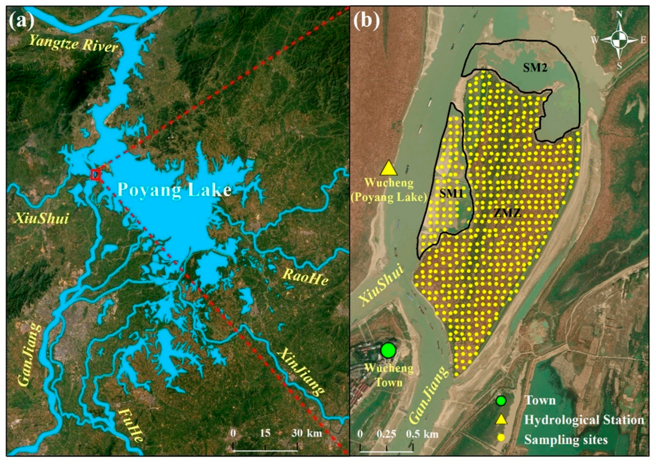
Figure 1. (a) Poyang Lake is situated on the southern bank of the Yangtze River. It receives inflows from five tributaries (i.e., Xinjiang, Fuhe, Ganjiang, Raohe, and Xiushui, commonly known as ‘Fiver Rivers’) and discharges into the Yangtze River. (b) A typical floodplain (Zengmizhou) was selected as the research area. It is located at the confluence of Xiushui and Ganjiang, north of Wucheng Town. Due to human sand mining activities in the early 21st century, the western (SM1 area) and northern (SM2 area) portions of the floodplain were excavated, while the remaining area, designated as the ZMZ area, maintains well-developed vegetation and has been unaffected by sand mining.
Remotesensing 18 01044 g001
Figure 2. Coverage distribution maps of (a) Carex spp. community and (b) T. lutarioriparia community in the ZMZ area of Zengmizhou; (c) NDVI distribution map of the floodplain on 12 November 2024, used to delineate the V1 zone (dominated by Carex spp.) and the V2 zone (mixed Carex–T. lutarioriparia community).
Remotesensing 18 01044 g002
Figure 3. Comparison of waterlines extracted by the object-based method (yellow solid lines) and terrain-measured contour lines (green solid lines) under (a) high water level (H = 15.40 m) and (b) low water level (H = 9.27 m). The red frame in (b) indicates an area where local depressions became hydraulically disconnected from the main channel, forming isolated water bodies that introduce discrepancies between the extracted waterline and the true topographic contour.
Remotesensing 18 01044 g003
Figure 4. Relationship between the number of remote sensing images used for topographic inversion and the elevation error rate (ΔE) of the reconstructed floodplain topography, based on the 179 spatially thinned validation dataset. Gray dots represent the ΔE for the entire floodplain (including both SM1 and ZMZ areas). The error bars indicate the range of ΔE values obtained from 8-fold spatial block cross-validation, providing a conservative estimate of uncertainty due to spatial autocorrelation. Triangles and squares indicate the ΔE for areas with elevations below 12 m (i.e., SM1) and above 12 m (i.e., ZMZ), respectively.
Remotesensing 18 01044 g004
Figure 5. Relationships between waterline-enclosed area (Sp) and the corresponding water level elevation (H) for Zengmizhou from 1987 to 2024, derived from 264 Landsat images using the object-based method. Different symbols represent five distinct periods in the floodplain’s topographic evolution with two excavation periods (triangles and squares) and three naturally stable periods (colored dots).
Remotesensing 18 01044 g005
Figure 6. Water level time series at the Wucheng (Poyang Lake) Hydrological Station from 1987 to 2024 (blue scatter points). Black dots indicate the acquisition times and corresponding water levels of the 264 remote sensing images. The entire period was divided into 15 sub-periods for DEM reconstruction (labeled P1 to P15; the numbers in parentheses indicate the number of images used for each sub-period). The two gray-shaded areas represent the sand mining excavation periods (January–August 2004 and November 2010–September 2011), which were excluded from accretion rate analysis. Five remote sensing images illustrate the morphological changes in Zengmizhou during different periods.
Remotesensing 18 01044 g006
Figure 7. Temporal variations in the mean elevation for different floodplain zones from 1987 to 2024: (a) ZMZ (natural zone, unaffected by sand mining), (b) SM1 (sand mining-affected zone), (c) V1 (Carex-dominated zone), and (d) V2 (mixed Carex–T. lutarioriparia zone). Red dots and lines represent the data and linear regression for pre-mining period (January 1987–December 2003); blue dots and lines represent the post-mining period; the gray dashed lines indicate the linear regression for the entire study period (1987–2024). For each regression line, the slope (k, in m day−1), coefficient of determination (r2), and p-value (testing whether the slope is significantly different from zero) are provided.
Remotesensing 18 01044 g007
Figure 8. Comparison of post-recession autumn NDVI between V1 (Carex-dominated zone) and V2 (mixed Carex–T. lutarioriparia zone) areas over 15 sub-periods (1987–2024). For each sub-period, one cloud-free Landsat image acquired during the post-recession autumn season (October–November) was selected, and the mean NDVI value for each zone was calculated by averaging the NDVI of all pixels within that zone’s boundaries.
Remotesensing 18 01044 g008
Figure 9. Temporal variations in combined sediment load of Ganjiang (Wan’an Station) and Xiushui Rivers (Wanjiapu Station) from 1985 to 2024. (a) Annual time series with linear regression (gray line) indicating a significant decreasing trend. (b) Cumulative sediment load segmented into three phases based on breakpoints at 1995 and 2005. Different symbols represent each phase, with linear regression lines fitted to each segment.
Remotesensing 18 01044 g009
Table 1. Accuracy assessment of waterlines extracted by different methods.
DateH (m)Area Error Rate (ΔS, %)Jaccard Coefficient (J)Kappa Coefficient (κ)Overall Accuracy (OA)
TSMOBMEDMSCMTSMOBMEDMSCMTSMOBMEDMSCMTSMOBMEDMSCM
28 December 2023☆◇*§†×7.12
12 November 20247.28
3 November 2024 7.42
28 January 2024 ☆◇*7.64
17 September 2024 8.10
2 November 2023☆◇*§†×9.278.675.523.7911.620.8200.8400.7100.8320.7470.9190.7320.8680.9070.9730.9000.960
18 November 20239.318.344.912.4410.320.8170.8280.7760.833
1 November 2023☆◇9.418.496.603.3614.660.8270.8510.7760.833
17 November 2023☆◇9.517.583.860.9611.770.8230.8320.8140.839
24 October 2023☆◇*§†9.765.794.221.9212.240.8410.8460.7890.843
14 February 2024☆◇*10.141.622.743.2712.860.8580.8780.8180.859
9 September 202410.491.001.1085.0719.580.8870.8840.5960.851
2 June 2023☆◇*§†10.561.350.136.522.980.8730.8910.8340.878
17 October 2023☆◇10.671.164.994.2116.920.8890.8830.8380.857
16 October 2023☆◇*§†10.900.289.205.784.740.9020.9140.8530.906
16 April 202310.950.941.018.054.850.9010.9070.8560.907
9 May 2023☆◇*§†×11.610.716.0113.667.600.9150.9430.8830.939
12 July 2023☆◇11.910.172.7187.4612.500.9150.9350.8740.933
1 September 2024☆◇*§†12.864.520.3587.2924.410.8680.8920.8550.8580.8110.8300.6980.8240.9400.9470.8930.953
28 May 2024☆◇*§†13.075.512.592.2020.380.8560.8690.8220.875
13 June 2024☆◇*§†×13.341.862.133.8716.370.8760.8650.8330.867
10 April 2024☆◇*§†13.824.841.3687.2519.310.8500.8740.8400.878
24 August 2024☆◇*§†×14.411.7213.4385.706.790.8500.7390.5840.811
21 June 2024☆◇*§†×15.4054.5032.6170.9860.700.5550.6860.5160.5960.6750.8800.6000.7470.8270.9400.8000.873
8 August 2024☆◇*§†×16.53
Mean value 6.27 5.5529.6715.290.8480.8610.7820.8530.7440.8760.6770.8130.8910.9530.8640.929
△○☆◇*§†※√× represent the composition of remote sensing images for the 25, 23, 21, 19, 17, 15, 13, 11, 9, and 7-image gradients, respectively, used for the topographic inversion accuracy test. TSM = Threshold Segmentation Method, OBM = Object-Based Method, EDM = Edge Detection Method, and SCM = Supervised Classification Method.
Disclaimer/Publisher’s Note: The statements, opinions and data contained in all publications are solely those of the individual author(s) and contributor(s) and not of MDPI and/or the editor(s). MDPI and/or the editor(s) disclaim responsibility for any injury to people or property resulting from any ideas, methods, instructions or products referred to in the content.