Global Spring–Autumn Phenology Coupling Inferred from Satellite Observations and Reanalysis-Based Climate Limitations

Highlights

What are the main findings?

• Spring and autumn phenology are positively linked globally, with autumn timing dominated by a direct effect rather than growing season climate mediation.
• Higher growing season water availability delays autumn senescence, but spring onset does not induce large-scale shifts in energy or water limitation regimes.

What are the implications of the main findings?

• Observed spring–autumn phenology correlations primarily reflect direct phenological coupling, rather than systematic climate mediation.
• Climate-mediated phenological effects are region-specific, identifying where land–atmosphere interactions modulate seasonal transitions.

Abstract

Spring and autumn phenology jointly regulate terrestrial carbon, water, and energy exchanges, yet the mechanisms linking seasonal transitions remain debated under increasing hydroclimatic stress. Here, we integrate satellite-derived phenology with reanalysis-based indicators of land–atmosphere coupling to examine how spring onset interacts with growing season controlling factors and how these interactions shape autumn senescence at the global scale. Globally, start-of-season (SOS) and end-of-season (EOS) timings are positively coupled, with later SOS generally followed by later EOS, and this relationship becomes stronger when only later-SOS years are considered. However, SOS does not induce coherent global shifts in growing season climate limitation. Piecewise structural equation modeling reveals that SOS influences EOS primarily through a direct phenological pathway, with a mean path coefficient of ~0.4 day·day⁻¹ explaining approximately 26% of global EOS variability. In contrast, energy and water-mediated pathways contribute smaller but spatially heterogeneous effects, together accounting for ~5% of explained variance on average. SOS–EOS coupling is strongest in water-limited regimes, particularly in grasslands and shrublands. Managed croplands exhibit distinct and more heterogeneous responses, reflecting partial decoupling of phenology from natural hydroclimatic constraints. Collectively, our results indicate that spring phenology exerts a robust but spatially variable influence on autumn timing, dominated by direct effects rather than indirect mediation through growing season climate limitations, with regional modulation imposed by background hydroclimatic conditions.

1. Introduction

Plant phenology regulates terrestrial carbon cycling and land–atmosphere interactions by controlling the timing and duration of seasonal vegetation activity. Spring leaf emergence initiates seasonal carbon uptake, evapotranspiration, and surface energy exchange, while autumn senescence marks the end of growing season and strongly constrains gross primary productivity (GPP) and nutrient cycling [1,2,3,4,5]. Through its control on canopy development and physiological activity, phenology also influences land surface properties such as albedo, roughness, and latent heat flux, thereby shaping land–atmosphere interactions across the growing season [1,6,7]. As vegetation develops, phenology-driven changes in evapotranspiration and soil moisture demand can further influence the balance between energy and water limitation, reinforcing seasonal feedbacks between ecosystems and climate [8,9,10,11,12].

Given these interactions, a large body of ecological and remote-sensing studies have identified carry-over effects linking spring and autumn phenology. Earlier spring onset (SOS) often extends canopy activity, enhances seasonal productivity, and can be associated with delayed autumn senescence (EOS) [5,13,14,15,16]. This spring–autumn coupling has been widely documented using satellite greenness indices and flux-site syntheses, particularly in temperate and boreal ecosystems [5,13,16,17]. At the same time, autumn senescence is known to be strongly constrained by growing season land surface conditions—including temperature, soil moisture, and radiation regimes—as well as their seasonal timing and variability [16,18,19,20,21,22]. These climatic controls vary substantially across regions, reflecting differences between energy-limited and water-limited environments as well as contrasting ecosystem functional strategies.

Recent evidence suggests that the strength and direction of spring–autumn coupling have become increasingly heterogeneous under rising hydroclimatic stress [15]. Satellite and observation-based studies report diminished trends or increased variability in autumn phenology since the early 2000s, alongside a growing sensitivity of EOS to drought and water stress [20,23,24,25]. These findings imply that while spring phenology remains influential, its effect on autumn timing may increasingly compete with or be overridden by growing season climate constraints, especially in water-limited regions. Earlier greening can increase evapotranspiration and accelerate soil moisture depletion, thereby intensifying late-season water stress and advancing autumn senescence in dry and semi-arid systems [8,15,26]. Observational and modeling studies further show that the sign and magnitude of spring–autumn coupling depend strongly on background hydroclimate: positive carry-over effects tend to dominate in humid, energy-limited regions, whereas neutral or negative effects emerge where soil moisture constraints are strong [21,24]. Consistent with this view, land surface and Earth system model simulations suggest that phenological shifts can alter the balance between energy and water limitation, potentially pushing ecosystems toward transitional coupling regimes under ongoing climate change [11,12,27].

Despite these advances, there is still a lack of a global, observation-based assessment of how spring phenology interacts with growing season controlling factors—specifically energy versus water limitation—and how these interactions shape autumn phenology across ecosystems and land cover types. Although autumn senescence is known to respond strongly to late-season land surface states [18,24,28], most large-scale studies treat these climatic controls independently from spring phenology. Meanwhile, modeling work suggests that SOS-induced shifts in energy–water partitioning may exert nonlinear and region-specific influences on EOS [11,12], but empirical evidence at the global scale remains limited.

In this study, we address these gaps by combining satellite-derived phenology with reanalysis-based indicators of climate limitation at 0.1° resolution. Using metrics that characterize energy limitation, water limitation, and their combined effects on latent heat flux, we examine whether and where spring onset timing modulates growing season controlling factors, and whether such modulation translates into changes in autumn senescence. Specifically, we ask: 1. How are growing season controlling factors (energy versus water limitation) related to remote sensing-based spring–autumn phenological relationships? 2. To what extent does the timing of spring onset influence growing season climate-limitation regimes? 3. How do these relationships vary across land cover types and hydroclimatic contexts? By explicitly linking spring phenology, growing season land surface states, and autumn senescence within a unified framework, this study provides new insights into when and where spring-driven effects dominate, and where coupling-mediated mechanisms emerge under increasing water limitation.

2. Materials and Methods

2.1. Start and End of Season

For global start-of-season (SOS) and end-of-season (EOS) estimates, we used the Moderate Resolution Imaging Spectroradiometer (MODIS) Global Vegetation Phenology product MCD12Q2 Version 6.1 [29], provided by the National Aeronautics and Space Administration (NASA, Washington, DC, USA). MCD12Q2 provides annual phenological transition dates at 500 m resolution, derived from MODIS observations from NASA’s Terra and Aqua satellites. Phenological metrics are generated from the two-band Enhanced Vegetation Index (EVI2), which is calculated from MODIS Nadir BRDF-Adjusted Reflectance (NBAR) time series. The 8-day NBAR-EVI2 observations are first interpolated to daily resolution using cubic smoothing splines to produce continuous seasonal trajectories from which phenophases are detected. Mid-Greenup and Mid-Greendown are defined as the day of year (DOY) when the smoothed annual EVI2 curve crosses 50% of its seasonal amplitude between the minimum and maximum EVI2.

In this study, we used the Mid-Greenup (SOS) and Mid-Greendown (EOS) metrics from the first detected annual growth cycle in the MCD12Q2 product. These metrics are defined using the 50% amplitude threshold, which reduces sensitivity to differences in absolute greenness and peak EVI2 values and improves cross-year and cross-site comparability in global applications [30,31]. Recent evaluations further demonstrate that MCD12Q2 phenology metrics exhibit high precision and low bias relative to extensive ground observations, supporting their suitability for long-term, large-scale phenology analyses [32]. All analyses in this study focus on the first detected growth cycle within each year, which contributes to the observed spatial variability in SOS and EOS differences, particularly in regions characterized by multiple seasonal greening events.

We applied the accompanying quality-assurance (QA) layer, which encodes retrieval confidence for each phenophase. Using Google Earth Engine (Google LLC, Mountain View, CA, USA), we parsed phase-specific QA bits and retained only retrievals flagged as “best” or “good,” masking all lower-confidence values. DOY estimates were then converted to days since January 1 for numerical consistency, and all phenology metrics were aggregated to a 0.1° (~11 km) grid via spatial averaging. Annual SOS and EOS estimates were extracted for 2001–2024.

2.2. Land Cover Dataset

We used the MODIS Land Cover Type product MCD12C1 Version 6.1 [33], which provides annual global land cover at 0.05° resolution. MCD12C1 is generated by spatially aggregating the 500 m land cover classification from MCD12Q1. The underlying land cover classes are derived from a supervised decision tree algorithm applied to combined Terra and Aqua MODIS surface reflectance time series, with training data drawn from high-resolution reference sites and global land cover inventories. Each 0.05° pixel includes both a majority land cover class and fractional class proportions.

We adopted the International Geosphere–Biosphere Programme (IGBP) scheme, which contains 17 land cover classes: ENF (evergreen needleleaf forest), EBF (evergreen broadleaf forest), DNF (deciduous needleleaf forest), DBF (deciduous broadleaf forest), MF (mixed forests), CSH (closed shrublands), OSH (open shrublands), WSA (woody savannas), SAV (savannas), GRA (grasslands), WET (permanent wetlands), CRO (croplands), URB (urban and built-up), CVM (cropland/natural vegetation mosaic), and BSV (barren or sparsely vegetated). For each 0.1° analysis grid cell (consisting of four 0.05° MCD12C1 pixels), we assigned the land cover type with the greatest cumulative area. We used the 2024 classification (Figure S1b), noting that interannual variations at this spatial scale are generally small and do not materially affect biome-level categories.

2.3. ERA5-Land Climate Data

We used the ERA5-Land reanalysis to obtain climate variables for the growing season controlling-factor analysis [34]. ERA5-Land is generated by a single replay of the land component of the European Centre for Medium-Range Weather Forecasts (ECMWF, Reading, UK) Reanalysis v5 (ERA5), providing a spatially enhanced representation of land-surface variables at 0.1° × 0.1° horizontal resolution. Compared with the standard ERA5 product, ERA5-Land offers improved spatial detail and internal consistency for land variables.

ERA5-Land is forced by atmospheric fields from ERA5 but is not coupled to the atmospheric model during its integration and does not directly assimilate land observations. As a result, variables such as snow water equivalent, snow temperature, soil temperature, and soil moisture are prognostically simulated, with observational influence entering only indirectly through the ERA5 atmospheric forcing.

In this study, we used latent heat flux (LH), shortwave solar radiation downward (SSRD), and total volumetric soil water (SW) from ERA5-Land. In ERA5-Land, LH is computed as the sum of evaporation and transpiration across sub-grid land-surface tiles; SSRD represents incoming solar radiation after accounting for atmospheric absorption and cloud reflection; and soil water content is simulated for four soil layers. Total volumetric soil water was obtained by summing water content across all four layers at each time step.

2.4. Ecosystem Limitation Index

We quantified the dominant environmental control on latent heat flux (LH) using the Ecosystem Limitation Index (ELI) following previous studies [12,35]. For each grid cell and each year, we computed Kendall’s rank correlations between monthly LH and (i) SSRD and (ii) SW for months with mean air temperature > 273 K. Prior to correlation analysis, we removed the seasonal cycle from each variable by subtracting the 2001–2024 monthly climatology.

The ELI was defined as:

ELI = CORR(SW,LH) − CORR(SSRD,LH),

where positive values indicate water limitation and negative values indicate energy limitation.

To characterize climate-limitation regimes, we evaluated ELI at two complementary temporal scales. First, annual ELI values were derived for each year using correlation coefficients computed across all months with air temperature > 273 K within that year. Second, long-term monthly correlations were calculated using all years combined (after deseasonalizing and detrending) to characterize seasonal variations in the dominant limitation factors.

A grid cell was classified as predominantly water-limited when both of the following criteria were satisfied:

• In at least 75% of years (≥18 of 24 years), annual ELI values were positive; and
• Within the long-term seasonal cycle, at least 75% of months exhibited positive ELI values.

An analogous set of criteria was applied to identify energy-limited regions.

2.5. Statistical and Comparative Analyses

To quantify SOS–EOS relationships, we first removed linear trends from each time series and then calculated Kendall rank correlation coefficients using the detrended data. Statistical significance was evaluated at the 10% level, and the Benjamini–Hochberg procedure was applied to control the false discovery rate [36]. The resulting spatial patterns of correlation and significance are shown in Figure S1a.

To examine how these relationships vary under different phenological and climatic conditions, we applied a quartile-based grouping strategy at each grid cell. For phenological comparisons, years were ranked according to SOS dates at each grid point; the earliest 25% were classified as “early SOS years,” and the latest 25% as “late SOS years.” Kendall correlations between SOS and EOS were then calculated separately for these subsets. To assess climatic modulation, years were additionally ranked by growing season total soil water. The lowest and highest quartiles (driest 25% and wettest 25%) were defined as dry and wet years, respectively.

For land cover comparisons, grid cells were grouped according to MODIS land cover classes (Section 2.2). Within each class, distributions of correlation coefficients, ELIs, and structural equation model (SEM) path coefficients were summarized using boxplots to facilitate cross-biome comparison.

2.6. Structural Equation Modeling

To quantify the direct and mediated effects of SOS on EOS through biophysical pathways, we applied piecewise structural equation modeling (SEM), a multivariate framework that partitions complex causal relationships into component linear models based on covariance structure [37,38]. Unlike traditional covariance-based SEM, piecewise SEM estimates paths using separate ordinary least-squares regressions, offering greater flexibility for non-normal data, modest sample sizes, and the spatial heterogeneity characteristic of ecological datasets.

Piecewise SEM is especially suitable for our grid-based analysis because it avoids the strong global-fit assumptions of full-information SEM and instead fits models independently at each grid cell. This allows spatial variability in climate–phenology relationships to emerge naturally while maintaining statistical robustness. For each 0.1° grid cell, we retained only locations with at least 17 valid annual observations across all variables after listwise deletion of missing values. This threshold was chosen to ensure stable SEM estimation given the relatively limited temporal coverage of MODIS (2001–2024). Following established SEM guidelines recommending a minimum of 5 observations per estimated parameter [37,39], 17 years represent a conservative lower bound for reliable parameter estimation. Grid cells not meeting this criterion were excluded from the SEM analysis.

Our model specified a direct path (SOS → EOS) and two parallel mediation pathways:

(1)

SOS → SSRDLH → EOS, representing the energy-mediated pathway, and

(2)

SOS → SWLH → EOS, representing the water-mediated pathway.

• Here, SSRDLH is the correlation between SSRD and LH, and SWLH is the correlation between soil water and LH.

The direct path coefficient represents the portion of SOS’s influence on EOS that remains after accounting for both seasonal energy and water limitations—effectively, the component of growing season length changes not explained by radiation or soil moisture constraints. The two indirect effects quantify biophysical mediation:

• Indirect effect 1 (SOS → SSRDLH → EOS) captures mediation through the radiation–energy pathway and reflects EOS shifts driven by changes in energy-controlled evapotranspiration following shifts in green-up.
• Indirect effect 2 (SOS → SWLH → EOS) captures mediation through the soil moisture pathway and reflects influences of moisture-driven changes in evapotranspiration on SOS–EOS relationships.

Indirect effects were computed as the product of their constituent path coefficients following standard mediation procedures [37,40]. Path coefficients (β) quantify the expected change in the dependent variable per unit change in the predictor, holding other variables constant [41]. Adjusted R² values were used to quantify pathway strength by indicating the proportion of variance in each dependent variable explained by its predictors. Model diagnostics, including variance inflation factors (VIF) and Durbin–Watson statistics, indicated low multicollinearity among predictors and independent residuals.

3. Results

3.1. Correlation Between Start and End of Season

Globally, end-of-season (EOS) timing is generally positively correlated with start-of-season (SOS) timing; however, statistically significant positive correlations are concentrated only in limited regions, including grasslands and shrublands in northern Russia, central South America, and central Africa (Figure S1a). Negative correlations occur primarily in northern China and the northeastern United States. Most land cover types exhibit an overall positive SOS–EOS correlation (Figure S1c), but negative correlations are more common in closed and open shrublands, croplands, and woody savannas, particularly in China and the United States. Evergreen forests also display a wider spread of correlation values and a greater prevalence of negative relationships than other forest types.

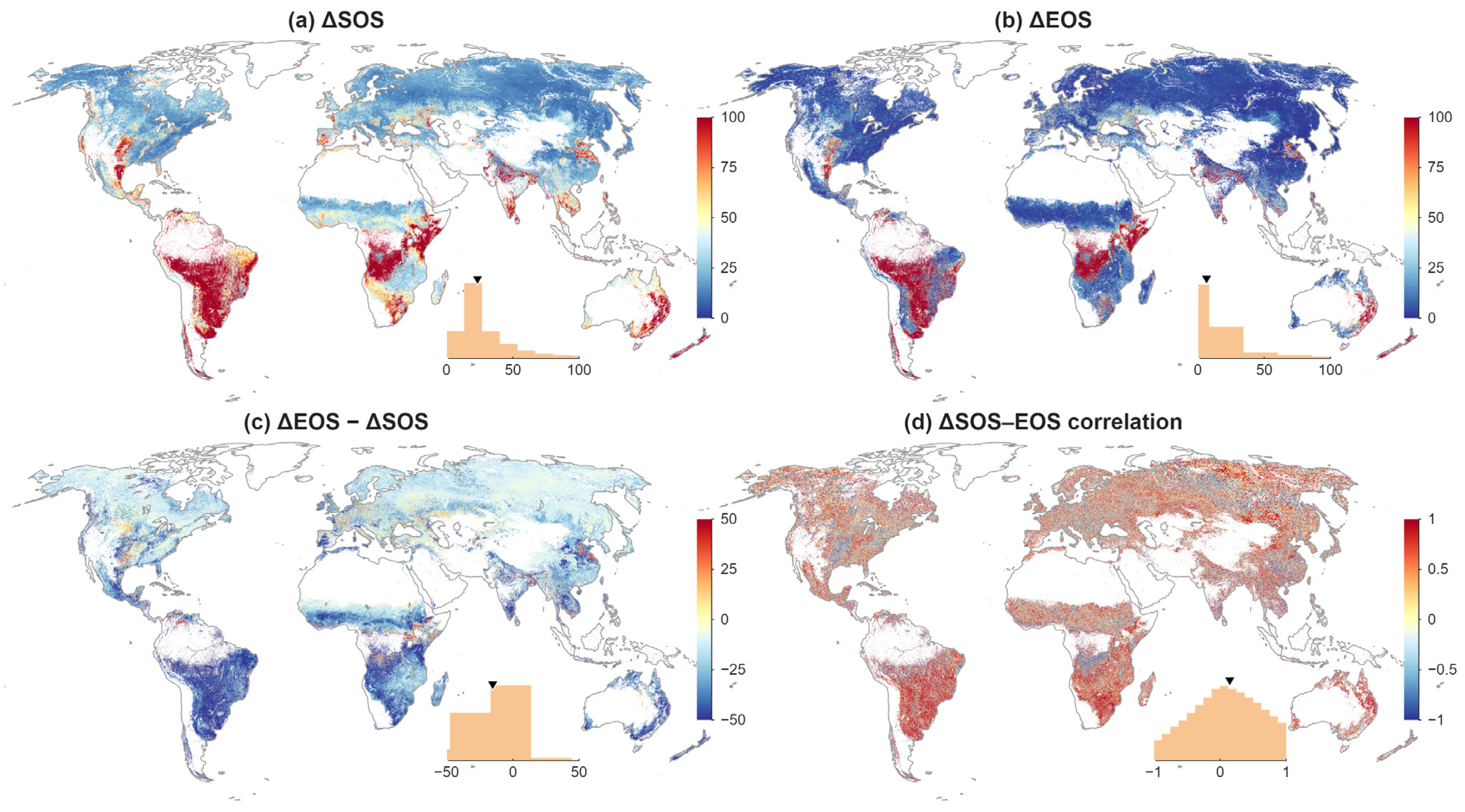
Years with later SOS generally also exhibit later EOS, although the magnitude of the shift is smaller for EOS than for SOS (Figure 1a–c). Globally, the median difference in SOS between early and late-SOS years is 42 days (Figure 1a), whereas the corresponding median difference in EOS is 12 days (Figure 1b), yielding a median ΔEOS–ΔSOS difference of −25 days (Figure 1c). Differences in SOS–EOS correlations also tend to be positive, with a median increase of 0.13 when only late-SOS years are considered (Figure 1d). Together, these results indicate that later spring onset is typically associated with later autumn senescence, but with a dampened response in EOS relative to SOS, and the SOS–EOS correlation is typically stronger in years characterized by later spring onset.

Further comparison of correlations between the earliest and latest 25% of SOS years shows that late-SOS years are associated with more positive SOS–EOS correlation coefficients across most locations (Figure S2a). Patterns vary across land cover types: evergreen needleleaf forests, deciduous broadleaf forests, woody savannas, grasslands, and managed lands display clearer increases in correlations during late-SOS years, whereas other land cover classes show weaker or less consistent differences (Figure S2e–r).

3.2. Growing Season Limiting Factors

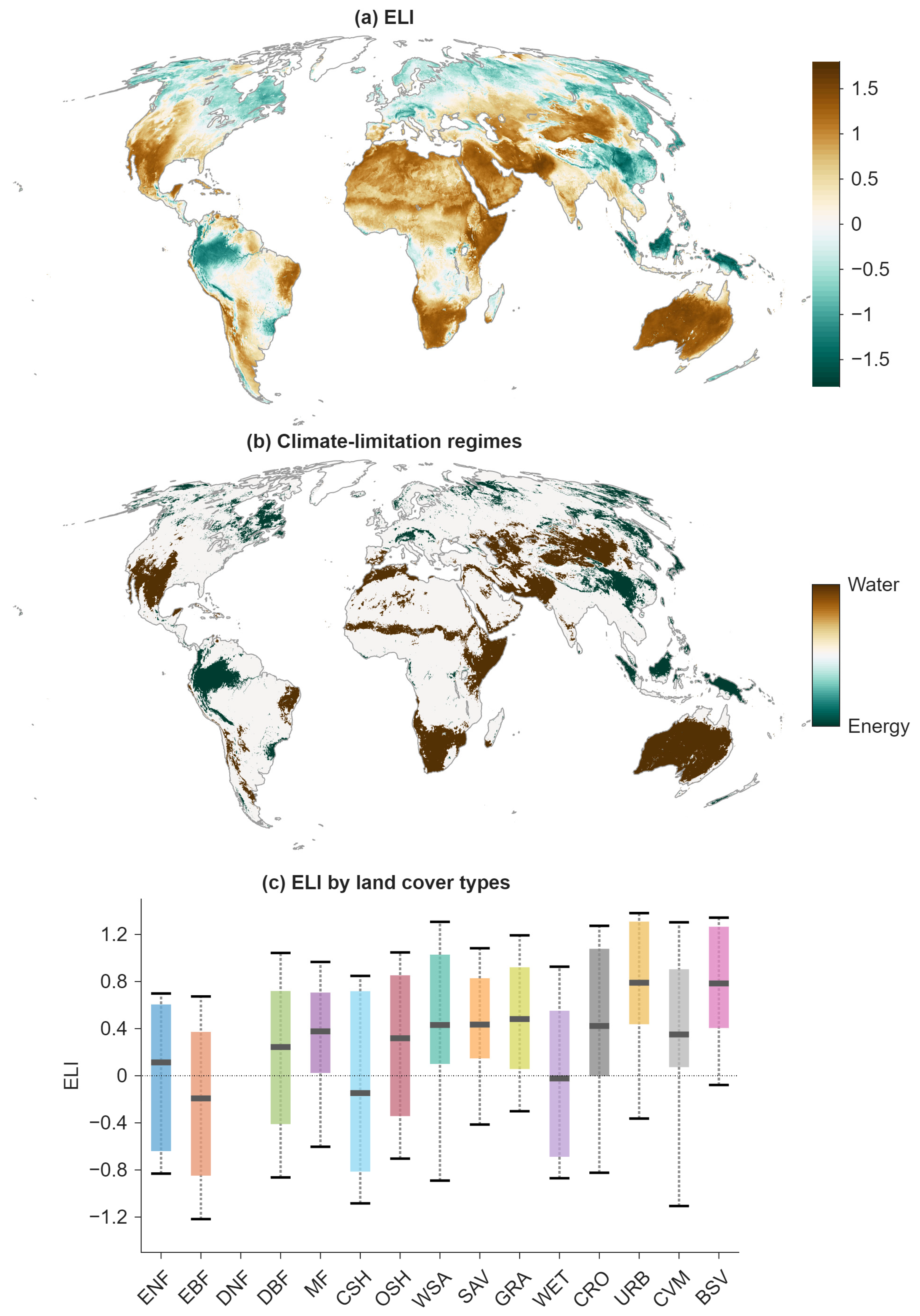
Growing season limiting factors vary substantially across the globe. Mid-to-high latitude regions of the Northern Hemisphere, the Amazon basin, and many Southeast Asian and tropical island regions are predominantly energy-limited, whereas most of the Southern Hemisphere is primarily water-limited, aside from several areas in central South America and central Africa (Figure 2a). Over annual to decadal timescales, however, many locations transition among different dominant limiting factors (Figure 2b). Regions that are consistently water-limited are mainly confined to arid and semi-arid grasslands such as the western United States, Australia, and central Asia, while consistently energy-limited regions occur primarily at high latitudes, high elevations, or within tropical rainforest ecosystems. ELI patterns also vary across land cover types, reflecting contrasting climate controls over different ecosystems (Figure 2c). Evergreen broadleaf forests, closed shrublands, and wetlands tend to be more energy-limited, whereas most other land cover types tend to be more moisture-limited through time.

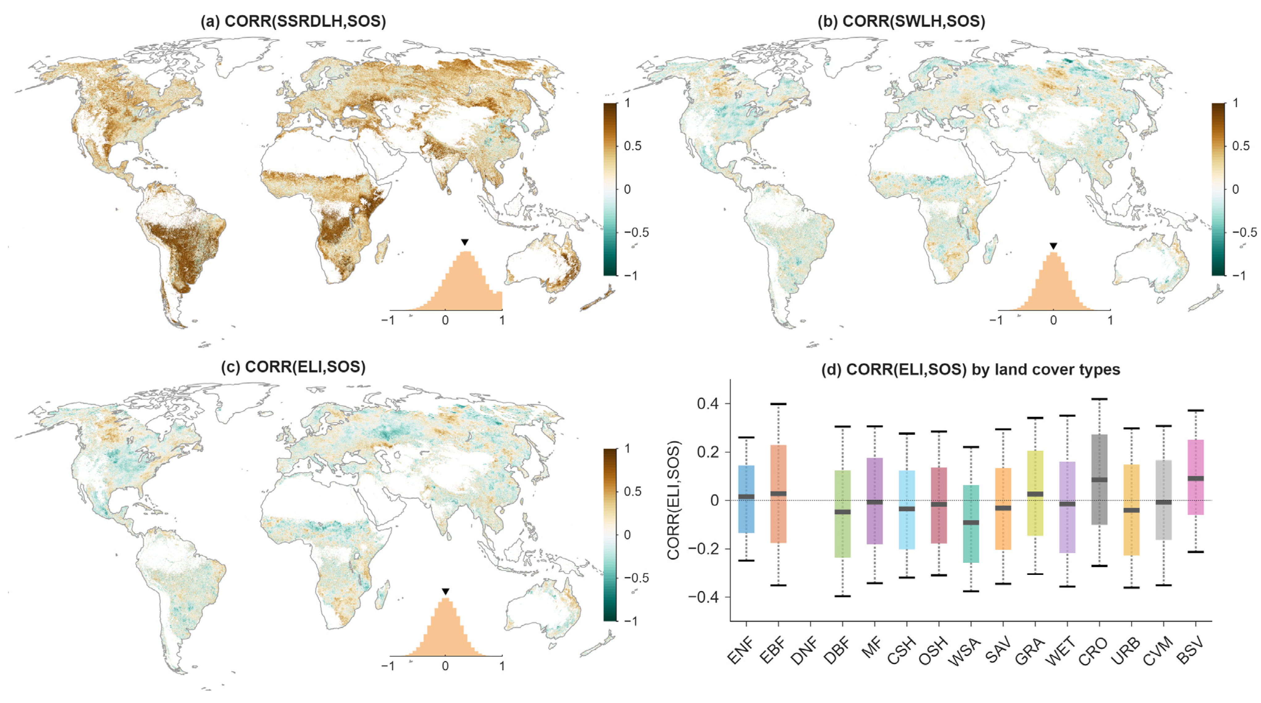
SOS shows a generally positive association with growing season energy limitation (CORR(LH, SSRD)), whereas its relationships with water limitation (CORR(LH, SW)) and overall ELI are more spatially heterogeneous (Figure 3). Globally, SOS is positively correlated with energy limitation, meaning earlier SOS tends to coincide with weaker energy control during the growing season, with exceptions in parts of the eastern United States, eastern China, and Europe (Figure 3a). SOS is typically negatively correlated with water limitation in moisture-rich regions (e.g., the eastern U.S. and high-latitude Northern Hemisphere), but correlations are more symmetrically distributed around zero overall (Figure 3b). Averaged across the globe, the mean correlation coefficient is 0.43 for correlations between SOS and energy limitation and close to 0 (<0.01) for water limitation and ELI. Spatially, SOS–ELI correlations resemble those of water limitation: correlations tend to be negative in moist regions—indicating that earlier SOS corresponds to stronger water limitation during the growing season—and positive in more arid regions (Figure 3c).

Comparisons between early and late SOS years reveal no globally consistent pattern, suggesting that SOS timing systematically regulates growing season limiting factors (Figure S3). Mean changes in energy limitation between early and late SOS years are small (mean −0.01; median −0.005), as are changes in water limitation (mean and median = 0.002). Consequently, changes in overall ELI are also minimal (mean 0.012; median 0.005).

Across land cover types, however, distinct ecosystem-specific responses emerge. Natural vegetation that is predominantly water-limited—such as deciduous broadleaf forests, woody savannas, and savannas—tends to show higher ELI (i.e., stronger moisture limitation) during early-SOS years (Figure S4g,k,i). In contrast, managed ecosystems, including croplands and sparsely vegetated areas, generally exhibit greater water limitation during late-SOS years (Figure S4o,r).

Spatial patterns in SOS–ELI correlations reinforce these tendencies: earlier SOS is associated with more positive SOS–ELI correlations in water-limited regions and more negative correlations in energy-limited regions (Figure S5b,c). These patterns are consistent across both energy limitation and water limitation. Certain land cover types—particularly mixed forests, woody savannas, and savannas—exhibit especially pronounced differences between early and late SOS years (Figure S5h,k,i).

3.3. Impacts of ELI and Dry/Wet Conditions on EOS, SOS, and Their Coupling

Correlations between EOS and ELI also vary across climate-limitation regimes (Figure S6). Compared with SOS, EOS shows weaker associations with growing season energy limitation: correlations are small in magnitude (mean ≈ 0.02) and centered near zero (Figure S6a). Correlations between EOS and water limitation, as well as EOS and overall ELI, are similarly centered around zero but with slightly negative means (≈−0.01; Figure S6b,c). Spatially, EOS tends to exhibit more positive correlations with energy limitation and more negative correlations with water limitation and ELI in energy-limited regions, including eastern North America, eastern and northern Asia, and northern Europe (Figure S6a–c).

Globally, SOS–EOS correlations are strongest in water-limited regions, with mean values of 0.30, 0.50, and 0.34 in energy-limited, water-limited, and variable-limitation regimes, respectively (Figure S7a), and these differences are statistically significant (p < 0.01, t-test). Across land cover types, the sensitivity of SOS–EOS coupling depends on both ecosystem functional type and its dominant climatic constraints. Vegetation typically experiencing stronger water limitation—evergreen needleleaf forests, closed and open shrublands, and grasslands—shows much stronger SOS–EOS correlations in water-limited regimes than in energy-limited regimes (Figure S7b,f,g,j). By contrast, temperature-limited vegetation types, including evergreen broadleaf and deciduous broadleaf forests, display higher SOS–EOS correlations in energy-limited regions (Figure S7c,d).

Wetter growing seasons generally lead to later EOS, especially in moisture-limited regions, although the links between this effect and changes in SOS are less clear. When years are stratified into wetter versus drier conditions, SOS shows no systematic shift (median ΔSOS = 0 days; Figure S8a). In contrast, EOS is consistently delayed in wetter years (median ΔEOS = 1.2 days; Figure S8b), resulting in longer growing seasons (median ΔLOS = 2.5 days; Figure S8c). Delayed EOS is most pronounced in arid and semi-arid regions, including southern Europe, the Great Plains, and tropical/subtropical regions of South America, Africa, and Australia. Overall, SOS–EOS correlations tend to be slightly more negative in wetter years, although the magnitude of this difference is small (−0.02; Figure S8d).

3.4. Spring–Autumn Phenology Coupling Based on Structural Equation Modeling

The piecewise SEM performed robustly despite the relatively short time series available at each grid cell (17–24 years). For each grid cell, we assessed potential multicollinearity using variance inflation factors (VIF) in the full EOS model (EOS ~ SOS + SSRDLH + SMLH). Median VIF values were low for all predictors—1.08 for SOS, 1.40 for water limitation, and 1.56 for energy limitation—and VIF > 5 occurred very rarely (~0.1% of vegetated grid cells for the limitation variables and <0.01% for SOS), indicating that collinearity is unlikely to bias path estimates. Residual autocorrelation was evaluated using the Durbin–Watson statistic, which was close to 2 across the globe (mean and median = 1.97), supporting the assumption of independent residuals and confirming that temporal dependence is minimal in the annual phenological and climate datasets [37]. Together, these diagnostics indicate that the SEM structure is statistically appropriate and that model coefficients are interpretable and stable across spatial domains.

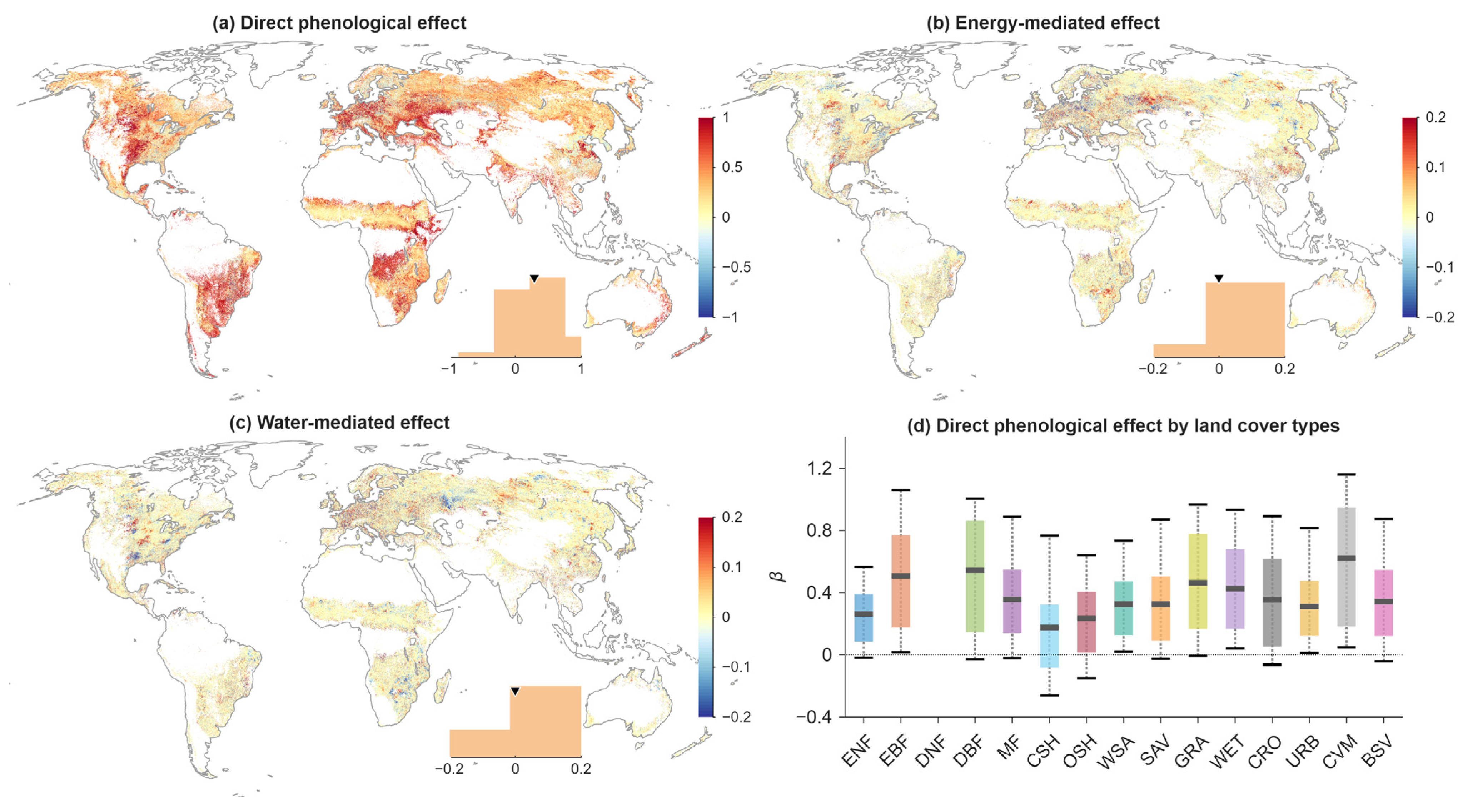
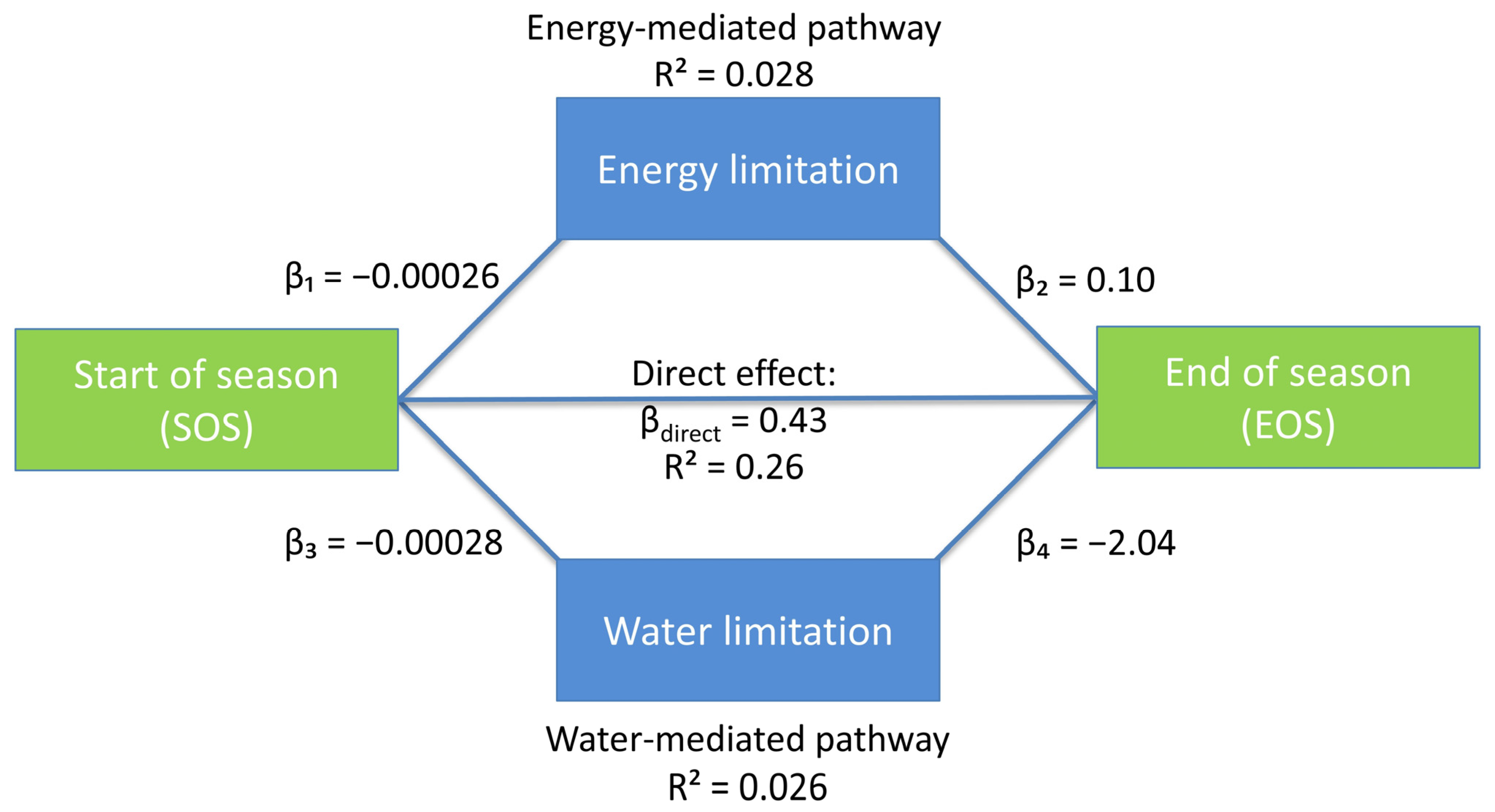
Overall, SOS exerts a positive influence on EOS, driven primarily by the direct phenological pathway (Figure 4). The direct SOS → EOS effect is consistently the strongest (mean = 0.43 day·day⁻¹, median = 0.39 day·day⁻¹). In contrast, both the energy and water-mediated pathways have mean and median values near zero, indicating limited but spatially variable mediation. Spatially, the largest positive direct effects occur over the Great Plains, southern Europe, South America, and Central Asia (Figure 4a). Energy-mediated effects are positive in regions such as the Great Plains and Eastern Europe, whereas portions of these same areas exhibit negative coefficients in the water-mediated pathway (Figure 4b,c). Positive water-mediated influences are most evident in the central Great Plains and central Siberia (Figure 4c). Across land cover types, negative direct coefficients are relatively rare but are most frequently found in natural shrubland ecosystems (Figure 4d).

We further examined the individual path coefficients associated with each segment of the SOS–EOS pathways. SOS effects on growing season limiting factors (energy and water limitations) are generally stronger in magnitude across the Northern Hemisphere, with particularly pronounced influences in the eastern United States, central Canada, eastern Europe, and central and eastern Siberia. Notably, the directional patterns for the two limitations are opposite: SOS tends to increase energy limitation in the southern Great Plains, eastern Europe, and eastern Siberia but decrease it in the northern Great Plains and central Siberia, whereas SOS effects on water limitation show the reverse pattern (Figure S9a,b).

In contrast, the influences of these limiting factors on EOS exhibit distinct spatial structures (Figure S9c,d). Energy and water-mediated effects on EOS are strongest in the southern Great Plains, southern Europe, southern Africa, and parts of South America. However, unlike the SOS → climate limitation pathways, the climate limitation → EOS pathways show mixed signs and no coherent regional gradient, reflecting the spatially heterogeneous roles of energy and soil moisture constraints in governing autumn phenology.

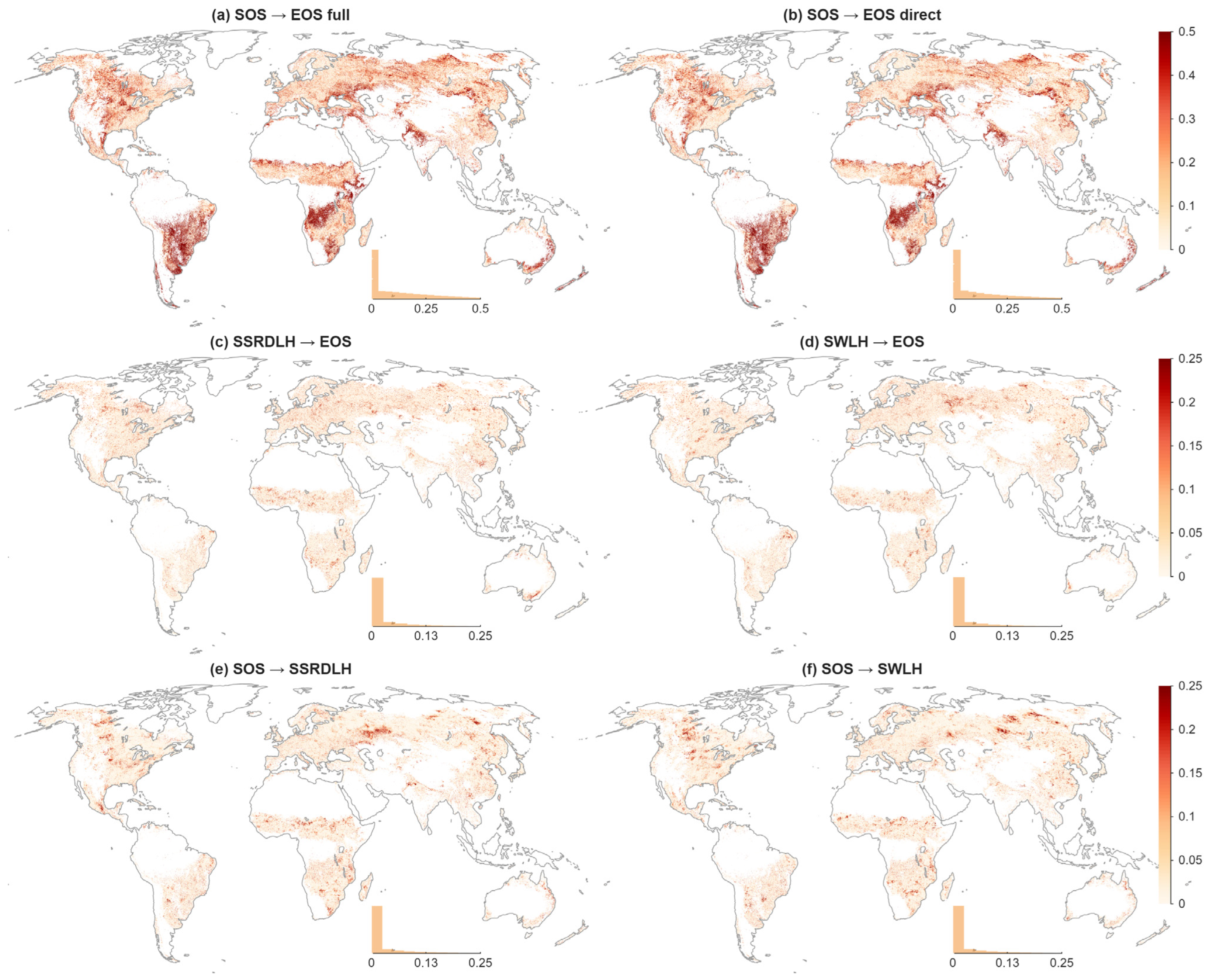
We also computed the explained variance at each grid point to illustrate how strongly SOS and climate-limitation pathways contribute to EOS variability worldwide (Figure 5 and Figure 6). Across all vegetated grid cells, the mean explained variance of EOS from the full SEM (i.e., the combined direct phenological pathway, SOS → EOS, plus the energy-mediated pathway, SOS → SSRDLH → EOS, and the water-mediated pathway, SOS → SWLH → EOS) is 0.27 (Figure 5a), with the direct phenological pathway alone accounting for most of this signal (mean adjusted R² = 0.26; Figure 5b and Figure 6). In contrast, mean explained variance from the energy and water-mediated pathways is modest (~0.02 for each; Figure 6), and SOS explains only slightly more variation in energy and water limitation themselves (~0.03 on average; Figure 5e,f).

These contributions vary substantially across regions. Higher R² values for the SOS → EOS pathway occur mainly in the Southern Hemisphere, particularly South America and Central Africa. In the Northern Hemisphere, elevated explained variance appears in northern forests of North America and Central Asia (Figure 5a,b). The energy-mediated pathway explains more EOS variance in high-latitude regions of the Northern Hemisphere, whereas the water-mediated pathway contributes more strongly in Eastern Europe (Figure 5c,d). SOS exerts stronger control on energy limitation in the Great Plains of North America, Eastern Europe, and Western Siberia, while its influence on water limitation is most pronounced in the Great Plains and Central Siberia (Figure 5e,f).

4. Discussion

Across the globe, spring and autumn phenology are positively coupled, with later spring onset (SOS) generally followed by later autumn senescence (EOS), and this relationship becomes stronger when only late-SOS years are considered. For growing season climate conditions, SOS is broadly associated with increased energy limitation, while its relationships with water limitation and the combined Ecosystem Limitation Index (ELI) are more spatially heterogeneous. Interannually, wetter growing seasons consistently delay EOS and lengthen the growing season, particularly in arid and semi-arid regions, yet early versus late SOS years do not induce coherent global shifts in growing season climate limitations, indicating that spring timing does not systematically regulate seasonal energy or water constraints. Piecewise SEM analysis clarifies the mechanisms underlying these patterns, showing that SOS influences EOS primarily through a direct effect, with a mean path coefficient of ~0.4 day·day⁻¹ that explains approximately 26% of global EOS variability. In contrast, energy and water-mediated pathways contribute much smaller but spatially variable effects, together accounting for around 5% of explained variance on average. These mediated influences are concentrated in specific regions—including the Great Plains, northeastern North America, eastern Europe, and western to northern Siberia—highlighting pronounced spatial heterogeneity in phenology–climate coupling. Collectively, these results indicate that while spring phenology exerts a robust influence on autumn timing, this influence is dominated by direct effects rather than by indirect mediation through growing season climate limitations, with ecosystem and region-specific modulation imposed by background hydroclimatic conditions.

Large-scale satellite and flux-site syntheses have frequently documented a spring–autumn carry-over effect, whereby earlier spring phenology extends canopy activity, enhances seasonal carbon uptake, and is often associated with delayed autumn senescence. For example, site-level flux syntheses demonstrated a biological carry-over of enhanced spring productivity into autumn carbon uptake [13]. Using AVHRR GIMMS NDVI time series, Liu et al. [16] further showed that delayed EOS contributed substantially to historical growing season lengthening and that earlier SOS was commonly associated with later EOS across temperate and boreal ecosystems. However, multiple recent studies indicate that this EOS delay has weakened in the later part of the observational record [22,24,25], coincident with diminished trends in both SOS and EOS during the warming hiatus [23]. Moreover, negative or weakened spring–autumn coupling has been observed in water-limited systems where early greening accelerates soil moisture depletion and intensifies late-season drought stress [8,21,25]. Within this broader context, our results indicate that positive SOS–EOS linkages dominate at the global scale, but their strength is spatially heterogeneous and often weak.

The dominance of the direct SOS–EOS pathway in our SEM suggests that autumn phenology is not primarily governed by concurrent growing season water or energy limitation. Instead, the direct effect likely represents aggregated biological processes not explicitly captured by ERA5-Land limitation metrics. Earlier SOS has been shown, in both experimental and observational studies, to accelerate early-season development and productivity, while also advancing leaf senescence later in the season [16,22,26]. Such patterns are often interpreted through internal source–sink interactions, particularly those associated with carbon assimilation and nutrient (especially nitrogen) storage dynamics [15,42,43]. Leaf lifespan itself may further contribute to the SOS–EOS relationship [44,45,46]. For instance, because leaf ageing is partly regulated by the accumulation of reactive oxygen species (ROS), earlier leaf-out can prolong exposure to solar radiation and oxidative stress, potentially accelerating ROS-mediated senescence processes [47,48,49]. At the same time, earlier greening also enhances evapotranspiration, accelerates soil moisture depletion, and increases exposure to late-season drought stress, thereby heightening vulnerability to water deficits and promoting earlier EOS in water-limited regions [8,15,24,25,26]. These moisture-mediated feedbacks can weaken or even reverse spring–autumn coupling under dry conditions, with EOS delays generally larger in humid regions than in arid ones [8,21,25]. The modest magnitude of climate-mediated pathways in our SEM therefore does not imply that climate is unimportant. Rather, it suggests that the net SOS–EOS linkage likely integrates multiple interacting mechanisms, and their combined signal appears as a direct effect within our statistical framework.

A key finding of this study is that SOS–EOS coupling is stronger in late-SOS years than in early-SOS years. When spring onset is early, EOS becomes less predictable and exhibits weaker coupling with SOS (Figure S2). This likely reflects competing influences: while early greening can promote extended carbon uptake [13,16,17], it also increases exposure to mid and late-season water stress or nutrient limitations [15,24,42,43]. In contrast, when SOS is delayed, EOS tends to shift correspondingly, producing stronger coupling that is not well explained by changes in growing season limitation factors. Importantly, early versus late-SOS years do not produce coherent global shifts in ELI (Figure S3). In moisture-limited regions, the relationship between SOS and ELI even reverses sign between early and late springs (Figure S5), suggesting nonlinear and state-dependent interactions rather than monotonic regulation of seasonal constraints. These results indicate that spring timing modulates the sensitivity of autumn phenology differently under early versus late onset conditions, highlighting an asymmetric and regime-dependent carry-over effect that extends beyond simple linear coupling.

Although SOS can modulate growing season climate limitation, large-scale patterns of the Ecosystem Limitation Index (ELI) are primarily determined by background climate conditions rather than interannual phenological variability. The influence of SOS on ELI is therefore not spatially uniform but emerges most clearly in ecosystems located near hydroclimatic thresholds, particularly semi-arid and transitional regions, where modest shifts in phenological timing can alter land–atmosphere coupling by pushing ecosystems across critical soil moisture or evaporative regimes [12,27,50,51]. Accordingly, we observe the strongest SOS-mediated effects on EOS in semi-arid and managed landscapes—including the Great Plains, parts of southern and eastern Europe, and southern Africa—where shallow soils, land management, and rapid canopy development amplify phenology-driven shifts in water and energy demand [52,53].

Biome-specific responses further highlight the importance of ecological context. Shrublands and grasslands, especially in the Southern Hemisphere, exhibit more frequent positive direct SOS–EOS coefficients in our analysis (Figure 4a,d and Figure S1a,c). This pattern is consistent with pulse-driven growth dynamics and high sensitivity to intra-seasonal moisture variability characteristic of dryland shrub ecosystems, where phenological development is often triggered by short precipitation events rather than sustained seasonal energy inputs [53,54]. Under such conditions, early spring onset does not necessarily translate into prolonged autumn activity if subsequent soil moisture becomes limiting, potentially weakening or reversing spring–autumn coupling. Managed croplands exhibit distinct and more heterogeneous responses. In these systems, planting dates, harvest schedules, irrigation, fertilization, and crop type selection partially decouple phenological timing from natural hydroclimatic constraints. Remote sensing studies demonstrate that agricultural phenology often reflects management calendars and multiple cropping cycles rather than purely climate-driven seasonal transitions [55,56]. The higher ELI observed in late-SOS cropland years in our results suggests that anthropogenic controls can override or reshape natural carry-over dynamics, leading to water limitation responses that differ from surrounding natural vegetation. This biome-dependent modulation provides additional ecological context for the stronger signals observed in shrublands and croplands and extends phenological coupling analysis beyond the temperate forest focus of many previous global studies.

The relatively weak linkages we identify between vegetation phenology and growing season climate-limitation factors likely reflect a combination of methodological and data-related uncertainties, arising from both the reanalysis-based climate products and remotely sensed phenology estimates. First, ERA5-Land is generated from a single, offline land surface model simulation forced by atmospheric reanalysis, in which vegetation phenology is prescribed rather than dynamically coupled to the surface energy and water balance [35]. As a result, interannual variations in phenology do not directly feed back into land–atmosphere exchanges within the model, and the influence of phenological variability on latent heat fluxes, radiation partitioning, and soil moisture is only indirectly reflected through meteorological forcing. This modeling structure likely dampens the sensitivity of energy and water limitation metrics to realistic phenological shifts, thereby attenuating detectable SOS-driven effects on growing season coupling.

Second, uncertainties in land surface phenology (LSP) derived from satellite observations further complicate attribution. Remotely sensed phenology products are known to be sensitive to sensor characteristics, vegetation indices, smoothing algorithms, and threshold definitions, with substantial discrepancies across datasets, especially in regions with complex canopy structure, sparse vegetation, or multiple growing seasons [30,57]. In tropical, semi-arid, and agricultural systems, phenological signals may reflect multiple green-up events, management practices, or moisture pulses rather than a single coherent growing season, increasing mismatch with model-based representations of seasonal climate limitation. In such regions, large SOS and EOS differences may partly reflect shifts between distinct growth cycles rather than changes within a single phenological trajectory, which can amplify apparent spring–autumn offsets. In addition, this study adopted a 50% amplitude threshold to define phenological transitions. Lower relative thresholds (e.g., 10%) may better capture phenological extremes or short-term responses to climate anomalies, particularly in water-limited or highly seasonal systems, but this increased sensitivity also raises susceptibility to noise, especially in areas affected by cloud contamination, low signal-to-noise ratios, or multiple growth cycles [31,58]. In addition, aggregating MODIS phenology (500 m) to the coarser ERA5-Land grid (0.1°) introduces scaling effects that smooth fine-scale heterogeneity, especially in fragmented landscapes. Spatial averaging can dampen sub-grid variability in vegetation indices and phenological timing, biasing transition dates toward earlier signals [31,59]. Multi-scale evaluations further show that such aggregation may attenuate temporal dynamics where fine-scale spatial and temporal variability interact, leading to underestimation of local phenological sensitivity [58]. Together, these limitations suggest that the modest climate-mediated effects identified here should be interpreted conservatively—not as evidence that phenology–climate coupling is negligible, but rather that its detection is constrained by current data-model inconsistencies and scale mismatches.

Future work should aim to better reconcile scale and process mismatches between phenology observations and climate-limitation metrics. One direction is to incorporate site-level observations that directly capture vegetation–atmosphere interactions, as well as targeted model experiments that explicitly test land-surface processes and phenological feedbacks [13]. From a modeling perspective, analyses based on fully coupled land–atmosphere simulations—where phenology actively feeds back on energy and water fluxes—would enable a more realistic quantification of phenology–climate coupling strength than reanalysis-based approaches alone [9,11]. Finally, extending this framework to examine lagged and multi-year legacy effects would help disentangle immediate phenological effects from longer-term ecological memory, providing a more complete picture of how phenological shifts propagate through ecosystems under continued climate change [15,25].

5. Conclusions

This study provides a global, observation-based assessment of how spring phenology interacts with growing season climate controls to shape autumn senescence. Using satellite-derived phenology and reanalysis-based indicators of energy and water limitation, we show that spring onset and autumn senescence are generally positively coupled worldwide, with later SOS tending to be followed by later EOS. However, structural equation modeling reveals that the direct SOS–EOS pathway explains approximately 26% of global EOS variability, whereas energy and water-mediated pathways contribute much smaller, though spatially heterogeneous, effects. These mediated influences are concentrated in specific hydroclimatic “hot spots,” including the Great Plains, northeastern North America, eastern Europe, and western to central Siberia. Importantly, our results show that while SOS is broadly associated with growing season energy limitation, it does not induce coherent global shifts in energy or water limitation regimes. Instead, background climate variability largely determines large-scale ecosystem limitation states, with spring phenology primarily modulating local land–atmosphere interactions where systems operate near critical thresholds. These findings provide process-based constraints for improving the representation of seasonal phenology coupling in land surface and Earth system models, and improve the interpretation of remotely sensed phenological shifts under changing hydroclimatic regimes. Future work should aim to better resolve scale and process mismatches between phenology observations and climate-limitation metrics by integrating site-level flux measurements, soil moisture observations, and coupled land–atmosphere model simulations in which phenology actively feeds back on surface fluxes. Extending this framework to account for lagged and multi-year legacy effects, as well as explicitly separating species-level and ecosystem-scale responses, will be essential for improving predictions of phenological sensitivity and land–atmosphere interactions under continued warming and water stress.

References

1. Richardson, A.D.; Keenan, T.F.; Migliavacca, M.; Ryu, Y.; Sonnentag, O.; Toomey, M. Climate change, phenology, and phenological control of vegetation feedbacks to the climate system. Agric. For. Meteorol. 2013, 169, 156–173. [Google Scholar] [CrossRef] [Scilit]
2. Piao, S.; Liu, Q.; Chen, A.; Janssens, I.A.; Fu, Y.; Dai, J.; Liu, L.; Lian, X.; Shen, M.; Zhu, X. Plant phenology and global climate change: Current progresses and challenges. Glob. Change Biol. 2019, 25, 1922–1940. [Google Scholar] [CrossRef] [Scilit]
3. Tang, J.; Körner, C.; Muraoka, H.; Piao, S.; Shen, M.; Thackeray, S.J.; Yang, X. Emerging opportunities and challenges in phenology: A review. Ecosphere 2016, 7, e01436. [Google Scholar] [CrossRef] [Scilit]
4. Piao, S.; Wang, X.; Park, T.; Chen, C.; Lian, X.; He, Y.; Bjerke, J.W.; Chen, A.; Ciais, P.; Tømmervik, H.; et al. Characteristics, drivers and feedbacks of global greening. Nat. Rev. Earth Environ. 2019, 1, 14–27. [Google Scholar] [CrossRef] [Scilit]
5. Jeong, S. Autumn greening in a warming climate. Nat. Clim. Change 2020, 10, 712–713. [Google Scholar] [CrossRef] [Scilit]
6. Penuelas, J.; Rutishauser, T.; Filella, I.; Peñuelas, J.; Rutishauser, T.; Filella, I. Phenology Feedbacks on Climate Change. Science 2009, 324, 887–888. [Google Scholar] [CrossRef] [Scilit]
7. Seneviratne, S.I.; Corti, T.; Davin, E.L.; Hirschi, M.; Jaeger, E.B.; Lehner, I.; Orlowsky, B.; Teuling, A.J. Investigating soil moisture-climate interactions in a changing climate: A review. Earth. Sci. Rev. 2010, 99, 125–161. [Google Scholar] [CrossRef] [Scilit]
8. Lian, X.; Piao, S.; Li, L.Z.X.; Li, Y.; Huntingford, C.; Ciais, P.; Cescatti, A.; Janssens, I.A.; Peñuelas, J.; Buermann, W.; et al. Summer soil drying exacerbated by earlier spring greening of northern vegetation. Sci. Adv. 2020, 6, eaax0255. [Google Scholar] [CrossRef] [Scilit]
9. Lian, X.; Jeong, S.; Park, C.-E.; Xu, H.; Li, L.Z.X.; Wang, T.; Gentine, P.; Peñuelas, J.; Piao, S. Biophysical impacts of northern vegetation changes on seasonal warming patterns. Nat. Commun. 2022, 13, 3925. [Google Scholar] [CrossRef] [Scilit]
10. Li, Y.; Li, Z.-L.; Wu, H.; Zhou, C.; Liu, X.; Leng, P.; Yang, P.; Wu, W.; Tang, R.; Shang, G.-F.; et al. Biophysical impacts of earth greening can substantially mitigate regional land surface temperature warming. Nat. Commun. 2023, 14, 121. [Google Scholar] [CrossRef] [Scilit]
11. Li, X.; Ault, T.; Richardson, A.D.; Carrillo, C.M.; Lawrence, D.M.; Lombardozzi, D.; Frolking, S.; Herrera, D.A.; Moon, M. Impacts of shifting phenology on boundary layer dynamics in North America in the CESM. Agric. For. Meteorol. 2023, 330, 109286. [Google Scholar] [CrossRef] [Scilit]
12. Denissen, J.M.C.; Teuling, A.J.; Pitman, A.J.; Koirala, S.; Migliavacca, M.; Li, W.; Reichstein, M.; Winkler, A.J.; Zhan, C.; Orth, R. Widespread shift from ecosystem energy to water limitation with climate change. Nat. Clim. Change 2022, 12, 677–684. [Google Scholar] [CrossRef] [Scilit]
13. Richardson, A.D.; Black, T.A.; Ciais, P.; Delbart, N.; Friedl, M.A.; Gobron, N.; Hollinger, D.Y.; Kutsch, W.L.; Longdoz, B.; Luyssaert, S.; et al. Influence of spring and autumn phenological transitions on forest ecosystem productivity. Philos. Trans. R. Soc. B Biol. Sci. 2010, 365, 3227–3246. [Google Scholar] [CrossRef] [Scilit] [PubMed]
14. Keenan, T.F.; Richardson, A.D. The timing of autumn senescence is affected by the timing of spring phenology: Implications for predictive models. Glob. Change Biol. 2015, 21, 2634–2641. [Google Scholar] [CrossRef] [Scilit]
15. Trugman, A.T.; Anderegg, L.D.L. Source vs sink limitations on tree growth: From physiological mechanisms to evolutionary constraints and terrestrial carbon cycle implications. New Phytol. 2025, 245, 966–981. [Google Scholar] [CrossRef] [Scilit]
16. Liu, Q.; Fu, Y.H.; Zhu, Z.; Liu, Y.; Liu, Z.; Huang, M.; Janssens, I.A.; Piao, S. Delayed autumn phenology in the Northern Hemisphere is related to change in both climate and spring phenology. Glob. Change Biol. 2016, 22, 3702–3711. [Google Scholar] [CrossRef] [Scilit]
17. Tang, D.; Xie, S.; Peng, J.; Sun, Y.; Degen, A.A.; Sun, Y.; Luo, J.; Li, Z.; Kuang, Y.; Wei, L.; et al. The Increased Effect of Spring Leaf Unfolding on Autumn Senescence in the Northern and Southern Hemispheres. Glob. Ecol. Biogeogr. 2025, 34, e70180. [Google Scholar] [CrossRef] [Scilit]
18. Moon, M.; Richardson, A.D.; O’Keefe, J.; Friedl, M.A. Senescence in temperate broadleaf trees exhibits species-specific dependence on photoperiod versus thermal forcing. Agric. For. Meteorol. 2022, 322, 109026. [Google Scholar] [CrossRef] [Scilit]
19. Wu, C.; Wang, X.; Wang, H.; Ciais, P.; Peñuelas, J.; Myneni, R.B.; Desai, A.R.; Gough, C.M.; Gonsamo, A.; Black, A.T.; et al. Contrasting responses of autumn-leaf senescence to daytime and night-time warming. Nat. Clim. Change 2018, 8, 1092–1096. [Google Scholar] [CrossRef] [Scilit]
20. Zhang, Y.; Hong, S.; Liu, Q.; Huntingford, C.; Peñuelas, J.; Rossi, S.; Myneni, R.B.; Piao, S. Autumn canopy senescence has slowed down with global warming since the 1980s in the Northern Hemisphere. Commun. Earth Environ. 2023, 4, 173. [Google Scholar] [CrossRef] [Scilit]
21. Ji, S.; Ren, S.; Zhang, X.; Liu, R.; Gao, Z.; Li, C.; Fang, L.; Chen, J.; Wang, X.; Wang, G.; et al. The role of developmental and climate factors in driving autumn phenology across the Northern Hemisphere. Agric. For. Meteorol. 2025, 368, 110548. [Google Scholar] [CrossRef] [Scilit]
22. Wu, Z.; Fu, Y.H.; Crowther, T.W.; Renner, S.S.; Vitasse, Y.; Mo, L.; Zou, Y.; Mirzagholi, L.; Li, M.; Rebindaine, D.; et al. Carry-over effects between spring and autumn phenology differ among the World’s biomes. Natl. Sci. Rev. 2026, 13, nwag082. [Google Scholar] [CrossRef] [Scilit] [PubMed]
23. Wang, X.; Xiao, J.; Li, X.; Cheng, G.; Ma, M.; Zhu, G.; Arain, M.A.; Black, T.A.; Jassal, R.S. No trends in spring and autumn phenology during the global warming hiatus. Nat. Commun. 2019, 10, 2389. [Google Scholar] [CrossRef] [Scilit] [PubMed]
24. Wu, C.; Peng, J.; Ciais, P.; Peñuelas, J.; Wang, H.; Beguería, S.; Black, T.A.; Jassal, R.S.; Zhang, X.; Yuan, W.; et al. Increased drought effects on the phenology of autumn leaf senescence. Nat. Clim. Change 2022, 12, 943–949. [Google Scholar] [CrossRef] [Scilit]
25. Lian, X.; Peñuelas, J.; Ryu, Y.; Piao, S.; Keenan, T.F.; Fang, J.; Yu, K.; Chen, A.; Zhang, Y.; Gentine, P. Diminishing carryover benefits of earlier spring vegetation growth. Nat. Ecol. Evol. 2024, 8, 218–228. [Google Scholar] [CrossRef] [Scilit]
26. Zani, D.; Crowther, T.W.; Mo, L.; Renner, S.S.; Zohner, C.M. Increased growing-season productivity drives earlier autumn leaf senescence in temperate trees. Science 2020, 370, 1066–1071. [Google Scholar] [CrossRef] [Scilit]
27. Hsu, H.; Dirmeyer, P.A. Soil moisture-evaporation coupling shifts into new gears under increasing CO2. Nat. Commun. 2023, 14, 1162. [Google Scholar] [CrossRef] [Scilit]
28. Lang, W.; Chen, X.; Liang, L.; Ren, S.; Qian, S. Geographic and climatic attributions of autumn land surface phenology spatial patterns in the temperate deciduous broadleaf forest of China. Remote Sens. 2019, 11, 1546. [Google Scholar] [CrossRef] [Scilit]
29. Friedl, M.; Gray, J.; Sulla-Menashe, D. MODIS/Terra+Aqua Land Cover Dynamics Yearly L3 Global 500m SIN Grid V061 [Data Set]. NASA Land Processes Distributed Active Archive Center. 2022. Available online: https://www.earthdata.nasa.gov/data/catalog/lpcloud-mcd12q2-061 (accessed on 25 June 2025).
30. White, M.A.; de Beurs, K.M.; Didan, K.; Inouye, D.W.; Richardson, A.D.; Jensen, O.P.; O’Keefe, J.; Zhang, G.; Nemani, R.R.; van Leeuwen, W.J.D.; et al. Intercomparison, interpretation, and assessment of spring phenology in North America estimated from remote sensing for 1982–2006. Glob. Change Biol. 2009, 15, 2335–2359. [Google Scholar] [CrossRef] [Scilit]
31. Zhang, X.; Wang, J.; Gao, F.; Liu, Y.; Schaaf, C.; Friedl, M.; Yu, Y.; Jayavelu, S.; Gray, J.; Liu, L.; et al. Exploration of scaling effects on coarse resolution land surface phenology. Remote Sens. Environ. 2017, 190, 318–330. [Google Scholar] [CrossRef] [Scilit]
32. Purdy, L.M.; Sang, Z.; Beaubien, E.; Hamann, A. Validating remotely sensed land surface phenology with leaf out records from a citizen science network. Int. J. Appl. Earth Obs. Geoinf. 2023, 116, 103148. [Google Scholar] [CrossRef] [Scilit]
33. Friedl, M.; Sulla-Menashe, D. MODIS/Terra+Aqua Land Cover Type Yearly L3 Global 0.05Deg CMG V061 [Data Set]. NASA Land Processes Distributed Active Archive Center. 2022. Available online: https://www.earthdata.nasa.gov/data/catalog/lpcloud-mcd12c1-061 (accessed on 25 June 2025).
34. Muñoz-Sabater, J.; Dutra, E.; Agustí-Panareda, A.; Albergel, C.; Arduini, G.; Balsamo, G.; Boussetta, S.; Choulga, M.; Harrigan, S.; Hersbach, H.; et al. ERA5-Land: A state-of-the-art global reanalysis dataset for land applications. Earth Syst. Sci. Data 2021, 13, 4349–4383. [Google Scholar] [CrossRef] [Scilit]
35. Denissen, J.M.C.; Teuling, A.J.; Reichstein, M.; Orth, R. Critical Soil Moisture Derived From Satellite Observations over Europe. J. Geophys. Res. Atmos. 2020, 125, e2019JD031672. [Google Scholar] [CrossRef] [Scilit]
36. Benjamini, Y.; Hochberg, Y. Controlling the False Discovery Rate: A Practical and Powerful Approach to Multiple Testing. J. R. Stat. Soc. Ser. B Methodol. 1995, 57, 289–300. [Google Scholar] [CrossRef] [Scilit]
37. Lefcheck, J.S. piecewiseSEM: Piecewise structural equation modelling in r for ecology, evolution, and systematics. Methods Ecol. Evol. 2016, 7, 573–579. [Google Scholar] [CrossRef] [Scilit]
38. McIntosh, A.R.; Bookstein, F.L.; Haxby, J.V.; Grady, C.L. Spatial pattern analysis of functional brain images using partial least squares. Neuroimage 1996, 3, 143–157. [Google Scholar]
39. Wolf, E.J.; Harrington, K.M.; Clark, S.L.; Miller, M.W. Sample size requirements for structural equation models: An evaluation of power, bias, and solution propriety. Educ. Psychol. Meas. 2013, 73, 913–934. [Google Scholar] [CrossRef] [Scilit]
40. Baron, R.M.; Kenny, D.A. The moderator–mediator variable distinction in social psychological research: Conceptual, strategic, and statistical considerations. J. Pers. Soc. Psychol. 1986, 51, 1173. [Google Scholar] [CrossRef]
41. Bollen, K.A. A new incremental fit index for general structural equation models. Sociol. Methods Res. 1989, 17, 303–316. [Google Scholar] [CrossRef] [Scilit]
42. Paul, M.J.; Foyer, C.H. Sink regulation of photosynthesis. J. Exp. Bot. 2001, 52, 1383–1400. [Google Scholar] [CrossRef] [Scilit]
43. Guitman, M.R.; Arnozis, P.A.; Barneix, A.J. Effect of source-sink relations and nitrogen nutrition on senescence and N remobilization in the flag leaf of wheat. Physiol. Plant. 1991, 82, 278–284. [Google Scholar] [CrossRef] [Scilit]
44. Zhang, Y.; Hong, S.; Peñuelas, J.; Xu, H.; Wang, K.; Zhang, Y.; Lian, X.; Piao, S. Weakened connection between spring leaf-out and autumn senescence in the Northern Hemisphere. Glob. Change Biol. 2024, 30, e17429. [Google Scholar] [CrossRef] [Scilit] [PubMed]
45. Kikuzawa, K.; Onoda, Y.; Wright, I.J.; Reich, P.B. Mechanisms underlying global temperature-related patterns in leaf longevity. Glob. Ecol. Biogeogr. 2013, 22, 982–993. [Google Scholar] [CrossRef] [Scilit]
46. Reich, P.B.; Walters, M.B.; Ellsworth, D.S. Leaf life-span in relation to leaf, plant, and stand characteristics among diverse ecosystems. Ecol. Monogr. 1992, 62, 365–392. [Google Scholar] [CrossRef] [Scilit]
47. Ruban, A.V.; Pascal, A.; Lee, P.J.; Robert, B.; Horton, P. Molecular configuration of xanthophyll cycle carotenoids in photosystem II antenna complexes. J. Biol. Chem. 2002, 277, 42937–42942. [Google Scholar] [CrossRef] [Scilit]
48. Close, D.C.; Beadle, C.L. The ecophysiology of foliar anthocyanin. Bot. Rev. 2003, 69, 149–161. [Google Scholar] [CrossRef] [Scilit]
49. Wu, Z.; Chen, S.; De Boeck, H.J.; Stenseth, N.C.; Tang, J.; Vitasse, Y.; Wang, S.; Zohner, C.; Fu, Y.H. Atmospheric brightening counteracts warming-induced delays in autumn phenology of temperate trees in Europe. Glob. Ecol. Biogeogr. 2021, 30, 2477–2487. [Google Scholar] [CrossRef] [Scilit]
50. Jonard, F.; Feldman, A.F.; Gianotti, D.J.S.; Entekhabi, D. Observed water and light limitation across global ecosystems. Biogeosciences 2022, 19, 5575–5590. [Google Scholar] [CrossRef] [Scilit]
51. Denissen, J.M.C.; Teuling, A.J.; Koirala, S.; Reichstein, M.; Balsamo, G.; Vogel, M.M.; Yu, X.; Orth, R. Intensified future heat extremes linked with increasing ecosystem water limitation. Earth Syst. Dyn. 2024, 15, 717–734. [Google Scholar] [CrossRef] [Scilit]
52. Stegehuis, A.I.; Vogel, M.M.; Vautard, R.; Ciais, P.; Teuling, A.J.; Seneviratne, S.I. Early summer soil moisture contribution to Western European summer warming. J. Geophys. Res. Atmos. 2021, 126, e2021JD034646. [Google Scholar] [CrossRef] [Scilit]
53. Dutra, A.C.; Srivastava, A.; Ganem, K.A.; Arai, E.; Huete, A.; Shimabukuro, Y.E. Remote sensing-based phenology of dryland vegetation: Contributions and perspectives in the Southern Hemisphere. Remote Sens. 2025, 17, 2503. [Google Scholar]
54. Wang, Y.; Tian, D.; Xiao, J.; Li, X.; Niu, S. Increasing drought sensitivity of plant photosynthetic phenology and physiology. Ecol. Indic. 2024, 166, 112469. [Google Scholar] [CrossRef] [Scilit]
55. Amin, E.; Belda, S.; Pipia, L.; Szantoi, Z.; El Baroudy, A.; Moreno, J.; Verrelst, J. Multi-season phenology mapping of Nile Delta croplands using time series of Sentinel-2 and Landsat 8 green LAI. Remote Sens. 2022, 14, 1812. [Google Scholar] [CrossRef] [Scilit] [PubMed]
56. Salinero-Delgado, M.; Estévez, J.; Pipia, L.; Belda, S.; Berger, K.; Gómez, V.P.; Verrelst, J. Monitoring cropland phenology on Google Earth Engine using gaussian process regression. Remote Sens. 2021, 14, 146. [Google Scholar]
57. Bolton, D.K.; Gray, J.M.; Melaas, E.K.; Moon, M.; Eklundh, L.; Friedl, M.A. Continental-scale land surface phenology from harmonized Landsat 8 and Sentinel-2 imagery. Remote Sens. Environ. 2020, 240, 111685. [Google Scholar] [CrossRef] [Scilit]
58. Park, D.S.; Newman, E.A.; Breckheimer, I.K. Scale gaps in landscape phenology: Challenges and opportunities. Trends Ecol. Evol. 2021, 36, 709–721. [Google Scholar] [CrossRef] [Scilit] [PubMed]
59. Fisher, J.I.; Mustard, J.F. Cross-scalar satellite phenology from ground, Landsat, and MODIS data. Remote Sens. Environ. 2007, 109, 261–273. [Google Scholar]
Figure 1. Differences in SOS–EOS relationships between early and late SOS years (defined as the earliest and latest 25% of SOS within each grid cell, 2001–2024). (a) SOS differences (days); (b) EOS differences (days); (c) differences between EOS and SOS shifts (b − a, days); (d) differences in SOS–EOS correlation coefficients. Inset histograms show distributions of mapped differences; black triangles denote medians.
Remotesensing 18 01002 g001
Figure 2. Ecosystem Limitation Index (ELI) and climate-limitation regimes. (a) Spatial distribution of ELI (positive: water-limited; negative: energy-limited). (b) Classification of water, energy, and variable-limitation regions (Section 2.4). (c) ELI distribution by land cover type. Central black lines indicate mean ELI; boxes show the interquartile range; whiskers represent the 10th and 90th percentiles. Land cover types include: ENF (evergreen needleleaf forest), EBF (evergreen broadleaf forest), DNF (deciduous needleleaf forest), DBF (deciduous broadleaf forest), MF (mixed forests), CSH (closed shrublands), OSH (open shrublands), WSA (woody savannas), SAV (savannas), GRA (grasslands), WET (permanent wetlands), CRO (croplands), URB (urban and built-up), CVM (cropland/natural vegetation mosaic), and BSV (barren or sparsely vegetated).
Remotesensing 18 01002 g002
Figure 3. Correlations between SOS and growing season climate limitation during 2001–2024. (a) SOS vs. energy limitation; (b) SOS vs. water limitation; (c) SOS vs. ELI. Inset histograms show distributions of mapped correlations; black triangles denote medians. (d) Distribution of SOS–ELI correlations by land cover type. Symbols and land cover color schemes are the same as in Figure 2c.
Remotesensing 18 01002 g003
Figure 4. SEM path coefficients linking SOS and EOS. (a) Direct pathway (SOS → EOS). (b) Energy-mediated pathway (SOS → SSRDLH → EOS). (c) Water-mediated pathway (SOS → SWLH → EOS). Inset histograms show distributions of mapped coefficients; black triangles denote medians. (d) Distribution of direct pathway coefficients by land cover types. Symbols and land cover color schemes follow those used in Figure 2c.
Remotesensing 18 01002 g004
Figure 5. Adjusted R2 values (variance explained) for each SEM pathway. (a) Total explained variance. (b) Variance in EOS explained directly by SOS. (c) Variance explained by energy limitation. (d) Variance explained by water limitation. (e) Variance in energy limitation explained by SOS. (f) Variance in water limitation explained by SOS. Inset histograms show distributions of mapped R2.
Remotesensing 18 01002 g005
Figure 6. Structural equation model linking SOS and EOS. Numbers indicate global mean path coefficients (β) and mean adjusted R2 (2001–2024). The direct path represents phenological influence independent of seasonal energy or water constraints. The indirect pathways represent mediation through energy and water.
Remotesensing 18 01002 g006
Disclaimer/Publisher’s Note: The statements, opinions and data contained in all publications are solely those of the individual author(s) and contributor(s) and not of MDPI and/or the editor(s). MDPI and/or the editor(s) disclaim responsibility for any injury to people or property resulting from any ideas, methods, instructions or products referred to in the content.