Full Polarimetric Scattering Matrix Estimation with Single-Channel Echoes via Time-Varying Polarization Modulation

Highlights

What are the main findings?

• Time-varying polarization modulation steers the transmit/receive states along predefined Poincaré sphere trajectories to inject known polarization tags into single-channel echoes, enabling full PSM estimation from limited observations.
• A compact observation model supports a least squares estimator with low-rank approximation, achieving high accuracy in PSM estimation, with polarization similarity approaching 1 and near-zero Pauli decomposition errors at an SNR of ≥−20 dB.

What are the implications of the main findings?

• This approach provides a practical pathway for acquiring full polarimetric scattering information on resource-constrained platforms, supporting target detection and recognition.
• The method’s robustness across various polarization trajectories and error conditions lays the foundation for reliable polarimetric analysis in real-world remote sensing applications.

Abstract

Polarimetric information is essential for scattering interpretation and target characterization in synthetic aperture radar (SAR) remote sensing, yet many resource-constrained platforms (e.g., small satellites and unmanned aerial vehicles (UAVs)) operate with limited polarization modes or even a single radio frequency (RF) chain, which limits full polarimetric scattering acquisition. To address this limitation, this paper proposes a single-channel framework for estimating the full polarization scattering matrix (PSM) enabled by time-varying polarization modulation. The transmit/receive polarization states are steered along predefined trajectories on the Poincaré sphere to generate time-varying polarization tags that are encoded into the received echoes through the target’s polarization-varying response. A compact observation model is then derived to relate the single-channel echoes, the known polarization tags, and the unknown PSM; based on this, the PSM is then estimated via a least squares formulation with a low-rank approximation. Simulation results demonstrate the robust reconstruction of the full polarimetric scattering matrix under diverse modulation trajectories. For arbitrarily chosen random point targets, when the signal-to-noise ratio (SNR) exceeds −20 dB, the polarimetric similarity coefficient approaches 1, and the estimation errors of Pauli power components converge toward zero. Furthermore, the method’s reliability is validated on distributed vegetation clutter. Quantitative metrics demonstrate near-perfect statistical consistency, with polarimetric entropy and alpha angle errors within 0.14%. Overall, the proposed approach provides a practical pathway to enhance the availability of full polarimetric scattering information under limited-observation conditions, confirming its feasibility for downstream analysis in complex natural scenes while maintaining a single radio frequency (RF) chain architecture augmented by a polarization modulator.

1. Introduction

Polarization, as an intrinsic property of electromagnetic (EM) waves beyond amplitude, phase, and frequency, describes the spatial motion trajectory of the electric field vector [1]. When the EM wave radiated by a radar antenna illuminates a target, the polarization state of the scattered echo will change with respect to the polarization state of the incident wave due to the target’s varying-polarization effect. Such polarization variations are closely related to the target’s physical attributes (e.g., size, structure, and material) and motion characteristics (e.g., orientation) [2]. Therefore, acquiring the target’s polarimetric response expands the target’s feature dimension, significantly enhancing radar capabilities in target detection [3,4,5,6,7], recognition [8,9,10,11], and anti-jamming [12,13,14].

A key parameter to describe polarization-dependent scattering is the polarimetric scattering matrix (PSM). Since Sinclair introduced this concept in 1946, the PSM has served as a complete mathematical representation of a target’s scattering response to incident waves of arbitrary polarization. In remote sensing, this description is operationalized primarily through polarimetric synthetic aperture radar (PolSAR), which enables interpretation of scattering mechanisms and target characterization over wide areas [15,16,17]. By exploiting polarization-dependent responses, PolSAR supports interpretable polarimetric descriptors and decomposition-based analyses [18,19,20,21], and it has been widely used in complex-scattering scenarios such as vegetation classification [22,23,24], ocean monitoring [25,26,27], and the recognition of man-made structures [28,29,30,31].

However, conventional fixed single-polarization architectures fundamentally limit these capabilities. In such systems, the scattering matrix is reduced to a single observable complex element (e.g., $S_{\mathrm{hh}}$ or $S_{\mathrm{vv}}$), while cross-polarization and complementary co-polarization components remain inaccessible [32,33,34]. This dimensional reduction prevents the application of advanced polarimetric analysis tools, such as Pauli or Cloude–Pottier H-$\alpha$ decompositions, thereby restricting the radar’s ability to distinguish between surface, double-bounce, and volume scattering mechanisms. Such information loss is particularly problematic for emerging applications involving small satellites and unmanned aerial vehicles (UAVs), where high-fidelity physical interpretation is required for reliable decision-making in high-revisit or tactical missions.

Despite the clear demand for full-polarimetric data, implementing traditional dual-RF-chain architectures on these compact platforms is often impractical. The duplication of transmitters, receivers, and high-speed analog-to-digital converters (ADCs) imposes prohibitive size, weight, power, and cost (SWaP-C) penalties [35,36,37]. This creates a significant gap between the scientific need for sophisticated scattering analysis and the strict hardware constraints of payload-limited platforms. To bridge this gap, it is essential to develop innovative architectures that can reconstruct full polarimetric information while maintaining a simplified, single-channel hardware backend.

Existing efforts to obtain polarimetric information under such constraints can be broadly grouped into three directions. The first relies on conventional multi-channel fully polarimetric architectures that directly measure all required channels through orthogonal transmit/receive configurations at the expense of multiple RF chains and stringent calibration requirements [6,38,39]. The second adopts reduced-dimensional observation schemes (e.g., dual-polarization or compact polarimetry) to alleviate hardware burden while retaining partial discriminative capability [40,41,42]; however, incomplete observations can limit the interpretation of scattering mechanisms, especially when decomposition-based analyses (e.g., Pauli or Krogager components) are required. The third direction attempts to recover missing polarimetric information from constrained observations via physics-based modeling, constrained optimization, or learning-based mappings [17,41,43]. Underdetermined SAR reconstruction has also been investigated in multi-channel elevation SAR, where prior structure or diversity is exploited to recover otherwise ambiguous parameters [44]. Yet, reduced observations fundamentally correspond to a lower-dimensional projection of the full PSM and cannot uniquely determine it without additional assumptions. Performance is often assessed mainly by pixel-wise reconstruction fidelity, which may not directly reflect whether mechanism-relevant polarimetric signatures are preserved.

These limitations motivate further exploration of full polarimetric information acquisition strategies that are better suited to resource-constrained platforms. To this end, we propose a PSM estimation framework enabled by time-varying polarization modulation in a single-channel architecture. Specifically, the transmit/receive polarization states are actively steered along a predefined trajectory on the Poincaré sphere, introducing known time-varying polarization “tags” into the received echoes through the target’s polarization-dependent response. We establish a compact observation model linking single-channel measurements, known polarization tags, and the unknown PSM, and we derive an unbiased estimator by exploiting the induced low-rank structure.

The main contributions of this work are threefold:

(1)

Single-channel full polarimetric acquisition: A practical single-channel framework for acquiring full polarimetric scattering information on resource-constrained platforms is proposed via time-varying polarization modulation.

(2)

Polarization tagging and PSM estimation: By steering the transmit/receive polarization states along predefined trajectories on the Poincaré sphere, a polarization-tagging mechanism is introduced. Under this mechanism, a compact observation model is established to relate the single-channel echoes to the known polarization tags and the unknown PSM, enabling PSM estimation via a least squares formulation with a low-rank approximation under limited observations.

(3)

Mechanism-preserving validation for PolSAR application: Not only matrix-domain accuracy but also scattering-mechanism preservation are assessed, with Pauli decomposition errors used to demonstrate reliable interpretability across different modulation trajectories and noise levels.

The rest of this paper is organized as follows. Section 2 illustrates the proposed single-channel full polarimetric scattering matrix estimation framework enabled by time-varying polarization modulation, including the observation model, the PSM estimator, a theoretical performance analysis, and the evaluation metrics for both PSM estimation accuracy and Pauli decomposition consistency. Section 3 presents the experimental verification and robustness analysis, where the impacts of signal-to-noise ratio (SNR), polarization trajectory geometry, polarimetric diversity, Doppler mismatch, and polarization modulation errors are systematically investigated. Finally, Section 4 discusses the results, and Section 5 concludes the paper and outlines potential directions for future work.

2. Methodology

2.1. Single-Channel Full Polarimetric Estimation via Time-Varying Polarization Modulation

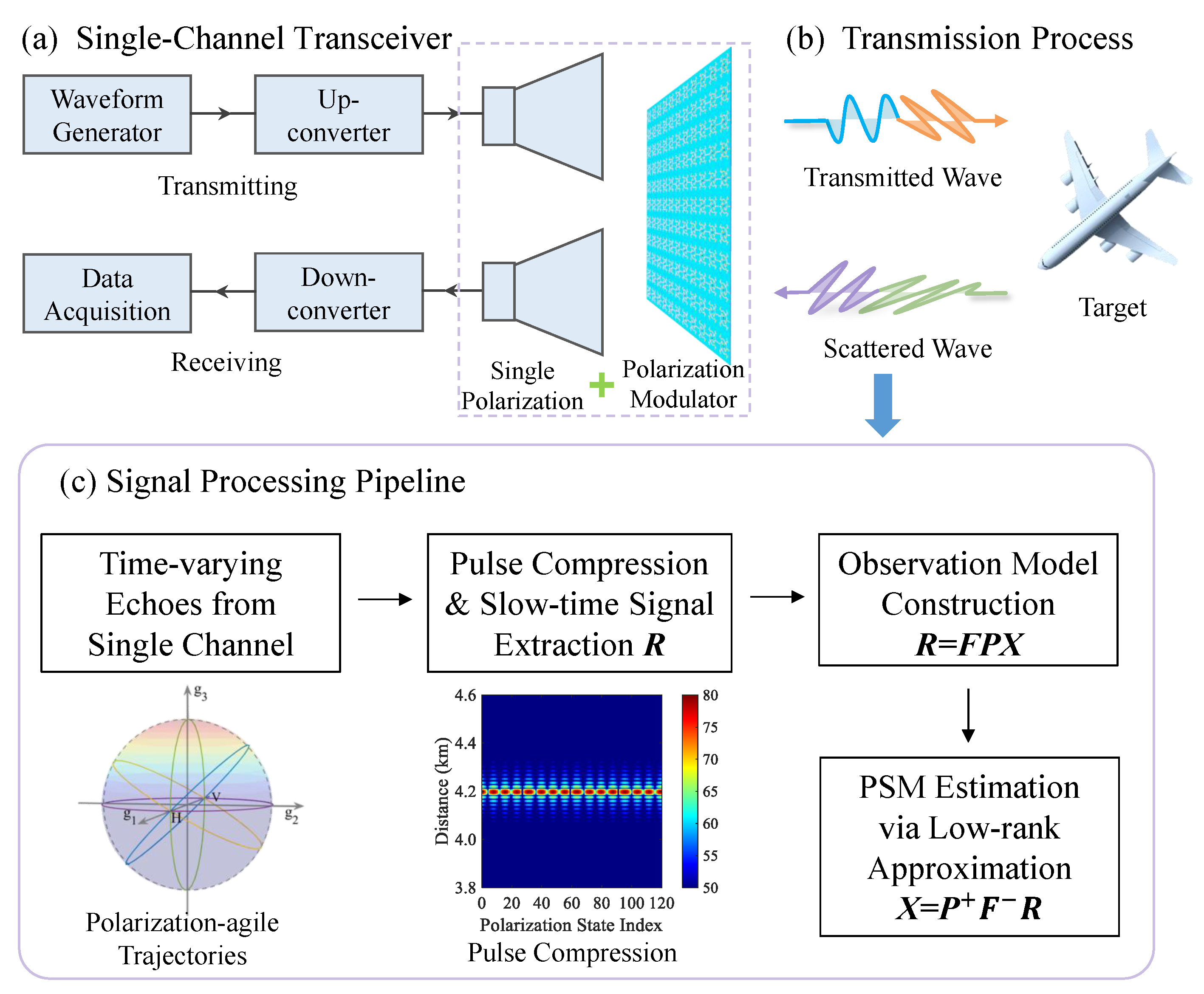
The conceptual diagram of the proposed PSM measurement method is illustrated in Figure 1.

To avoid conceptual ambiguity, it is necessary to emphasize that the term “Single-Channel” in this study refers exclusively to the utilization of a single RF transceiver hardware chain. It does not imply that a fixed, single-polarization wave (e.g., pure Horizontal (H) or pure Vertical (V)) is transmitted. As illustrated in Figure 1a, a polarization modulator integrated into the single-channel transceiver transforms the baseline polarization into a sequence of controlled, time-varying states, thereby embedding polarimetric diversity into the radar signal. Consequently, the signal radiated at any given pulse n is a deliberately synthesized composite wave containing both H and V components simultaneously.

Figure 1b depicts the EM wave propagation and corresponding polarization evolution. Because the incident wave consists of mixed polarizations, its interaction with the target inherently couples with all elements of the target’s intrinsic polarimetric scattering matrix (PSM) (i.e., $S_{\mathrm{hh}},S_{\mathrm{hv}},S_{\mathrm{vh}},S_{\mathrm{vv}}$). Upon reception, the composite echo wave is projected back through the modulator into the single RF chain, yielding a scalar voltage that encapsulates the full polarimetric information.

After matched filtering, the pulse-compressed peak fluctuates periodically in accordance with the time-varying polarization modulation, exhibiting the peak-to-trough amplitude behavior shown in Figure 1c. By extracting these sequence echoes over one complete polarization trajectory period, we can formulate a polarization-modulated observation equation. This equation bridges the single-channel measurements, the known polarization modulation matrix, and the unknown scattering matrix. Ultimately, the elements of the PSM can be accurately estimated using the least squares method.

2.2. Observation Model and PSM Estimator

Assuming the radar signal generator produces a baseband linear frequency modulated (LFM) signal, denoted as $e\left(t\right)$, it can be expressed as [5]

$$\mathit{e}\left(\mathit{t}\right)=rect\left({\displaystyle \frac{\mathit{t}}{{\mathit{T}}_{\mathit{p}}}}\right){\mathrm{e}}^{\mathrm{j}\pi \mathit{k}{\mathit{t}}^{\mathit{2}}},$$

(1)

where $rect(·)$ denotes the rectangular pulse function, $T_p$ is the pulse width, and k represents the chirp rate. The signal bandwidth is given by $B=k{T}_p$.

After upconversion, the signal can be expressed as

$$\mathit{s}\left(\mathit{t}\right)=\mathit{e}\left(\mathit{t}\right){\mathrm{e}}^{\mathrm{j}\mathit{2}\pi {\mathit{f}}_{\mathit{c}}\mathit{t}},$$

(2)

where $f_c$ is the carrier frequency.

When the polarization switching instant coincides with the pulse repetition interval (PRI), the polarization state ${\mathit{h}}_{T,n}$ remains constant for the duration of each corresponding pulse. The transmitted signal of the n-th pulse can be written as

$${\mathit{x}}_n\left(t\right)={\mathit{h}}_{T,n}{s}_n\left(t\right),n=1,2,\dots ,N,$$

(3)

where N is the number of distinct polarization states within one polarization trajectory cycle, and ${\mathit{h}}_{T,n}$ denotes the polarization state along a predefined polarization trajectory, which is expressed as a unit Jones vector ${\mathit{h}}_{T,n}={\left[cos{\gamma }_{n}sin{\gamma }_n{\mathrm{e}}^{\mathrm{j}{\varphi }_n}\right]}^{\mathrm{T}}$. Here, $\gamma$ is defined as polarization angle, and $\varphi$ is defined as phase difference.

Assuming the target’s scattering characteristics remain constant over the radar signal bandwidth and the coherent processing interval (CPI), its scattering matrix is denoted by S [2]:

$$\mathbf{S}=\left[\begin{array}{cc}{S}_{\mathrm{hh}}& S_{\mathrm{hv}}\\ S_{\mathrm{vh}}& S_{\mathrm{vv}}\end{array}\right].$$

(4)

This matrix describes the linear transformation of the incident polarization vector by the target in the backward direction.

The transmitted EM wave illuminates the target, and after being scattered by the target, the radar echo of the n-th pulse can be expressed as

$$\begin{array}{cc}\hfill {\mathit{y}}_n\left(t\right)& =\mathbf{S}{\mathit{h}}_{T,n}{s}_n\left(t-{\tau }_n\right)\hfill \\ \hfill & =\left[\begin{array}{c}cos{\gamma }_n{S}_{\mathrm{hh}}+sin{\gamma }_n{\mathrm{e}}^{\mathrm{j}{\varphi }_n}{S}_{\mathrm{hv}}\\ cos{\gamma }_n{S}_{\mathrm{vh}}+sin{\gamma }_n{\mathrm{e}}^{\mathrm{j}{\varphi }_n}{S}_{\mathrm{vv}}\end{array}\right]s_n\left(t-{\tau }_n\right),\hfill \end{array}$$

(5)

where ${\tau }_n=2R_0/c+2v_d(n-1)T/c$ denotes the time delay of the n-th pulse echo. Here, $R_0$ is the initial range between the radar and target, T is the PRI, and $v_d$ is the radial velocity of the target relative to the radar, which relates to the Doppler frequency $f_d$ by $f_d=-2v_d{f}_c/c$. The constant c represents the speed of light. Note that since the incident wave $h_{T,n}$ is a composite state containing both H and V components (as defined in Equation (3)), its interaction with the target physically couples with all elements of the PSM, making the full PSM in Equation (5) not a theoretical assumption, but a direct physical consequence of the modulated transmission.

At the receiver, according to antenna reciprocity, the receiving antenna also acquires the target signal following the same polarization-agile scheme along the orbit. The target echo signal entering the radar receiver is

$$v_n\left(t\right)={\mathit{h}}_{R,n}^{\mathrm{T}}\mathbf{S}{\mathit{h}}_{T,n}{s}_n\left(t-{\tau }_n\right),$$

(6)

where ${\mathit{h}}_{R,n}$ denotes the radar receiving polarization state. When inter-pulse polarization modulation is applied, the polarization-trajectory period is $T_{\mathrm{orbit}}=NT$, i.e., one trajectory cycle spans N pulses. Since the pulse width is much shorter than the polarization switching time, according to the radar “stop-and-go” model, the polarization state variation can be discretized as inter-pulse hopping, with the polarization state held constant (frozen) within a single pulse, yielding ${\mathit{h}}_{R,n}={\mathit{h}}_{T,n}$.

Assuming monostatic operation and reciprocity, we have $S_{\mathrm{hv}}=S_{\mathrm{vh}}$. Under this condition, the echo of the n-th pulse in Equation (6) can be expanded as follows:

$$\begin{array}{cc}\hfill v_n\left(t\right)& ={\left[\begin{array}{c}cos{\gamma }_n\\ sin{\gamma }_n{\mathrm{e}}^{\mathrm{j}{\varphi }_n}\end{array}\right]}^{\mathrm{T}}\left[\begin{array}{cc}{S}_{\mathrm{hh}}& S_{\mathrm{hv}}\\ S_{\mathrm{vh}}& S_{\mathrm{vv}}\end{array}\right]\left[\begin{array}{c}cos{\gamma }_n\\ sin{\gamma }_n{\mathrm{e}}^{\mathrm{j}{\varphi }_n}\end{array}\right]s_n\left(t-{\tau }_n\right)\hfill \\ \hfill & =P_n{s}_n\left(t-{\tau }_n\right).\hfill \end{array}$$

(7)

Here, let $P_n={cos}^2{\gamma }_n{S}_{\mathrm{hh}}+2sin{\gamma }_{n}cos{\gamma }_n{\mathrm{e}}^{\mathrm{j}{\varphi }_n}{S}_{\mathrm{hv}}+{sin}^2{\gamma }_n{\mathrm{e}}^{\mathrm{j}2{\varphi }_n}{S}_{\mathrm{vv}}$. This term is determined jointly by the polarization-agile modulation factor and the target’s polarimetric scattering properties.

Within one complete polarization orbit cycle, the sequence of received radar echo pulses is

$$v\left(t\right)=\sum _{n=1}^N{v}_n\left(t\right).$$

(8)

In the radar signal processing stage, the received target echo sequence is first down-converted

$$\begin{array}{cc}\hfill z\left(t\right)& =v\left(t\right)·\left(q\left(t\right)\right)*\hfill \\ \hfill & =\sum _{n=1}^N{P}_{n}e\left(t-{\tau }_n\right){\mathrm{e}}^{\mathrm{j}2\pi f_d(n-1)T},\hfill \end{array}$$

(9)

where $q\left(t\right)={\mathrm{e}}^{\mathrm{j}2\pi f_{c}t}$ denotes the local oscillator signal.

Subsequently, matched filtering is applied to the baseband signal. The result is given by

$$R\left(t\right)=z\left(t\right)\ast h\left(t\right)=\sum _{n=1}^N{R}_n\left(t\right),$$

(10)

where $h\left(t\right)$ is the matched filter impulse response, related to the radar baseband signal $e\left(t\right)$ by $h\left(t\right)=e*(-t)$. $R_n\left(t\right)$ represents the matched filter output for the n-th pulse echo. The pulse compression output peak occurs at $t={\tau }_n$, and the corresponding normalized peak value is

$$R_n\left(t\right)=P_n{\mathrm{e}}^{\mathrm{j}2\pi f_d(n-1)T}.$$

(11)

For the pulse compression outputs from one polarization orbit cycle, the peak value from each pulse is extracted. Transforming this into matrix form yields

$$\left[\begin{array}{c}{R}_1\left(t\right)\\ R_2\left(t\right)\\ ⋮\\ R_N\left(t\right)\end{array}\right]=\left[\begin{array}{cccc}1& 0& \dots & 0\\ 0& {\mathrm{e}}^{\mathrm{j}2\pi f_{d}T}& \dots & 0\\ ⋮& ⋮& \ddots & ⋮\\ 0& 0& \dots & {\mathrm{e}}^{\mathrm{j}2\pi f_d(N-1)T}\end{array}\right]\left[\begin{array}{ccc}{cos}^2{\gamma }_1& sin\left(2{\gamma }_1\right){\mathrm{e}}^{\mathrm{j}{\varphi }_1}& {sin}^2{\gamma }_1{\mathrm{e}}^{\mathrm{j}2{\varphi }_1}\\ {cos}^2{\gamma }_2& sin\left(2{\gamma }_2\right){\mathrm{e}}^{\mathrm{j}{\varphi }_2}& {sin}^2{\gamma }_2{\mathrm{e}}^{\mathrm{j}2{\varphi }_2}\\ ⋮& ⋮& ⋮\\ {cos}^2{\gamma }_N& sin\left(2{\gamma }_N\right){\mathrm{e}}^{\mathrm{j}{\varphi }_N}& {sin}^2{\gamma }_N{\mathrm{e}}^{\mathrm{j}2{\varphi }_N}\end{array}\right]\left[\begin{array}{c}{S}_{\mathrm{hh}}\\ S_{\mathrm{hv}}\\ S_{\mathrm{vv}}\end{array}\right].$$

(12)

The above equation is denoted as $\mathit{R}=\mathit{FPX}$, where $\mathit{R}$ is the vector of echo pulse-compression peak values, $\mathit{F}=\mathrm{diag}(1,{\mathrm{e}}^{\mathrm{j}2\pi f_{d}T},\cdots ,{\mathrm{e}}^{\mathrm{j}2\pi f_d(N-1)T})$ is the diagonal matrix formed by the Doppler frequency shifts, $\mathit{P}\in {\mathbb{C}}^{N\times 3}$ is the polarization modulation matrix constructed from the discrete polarization states along the polarization orbit, and $\mathbf{X}={\left[S_{\mathrm{hh}}{S}_{\mathrm{hv}}{S}_{\mathrm{vv}}\right]}^{\mathrm{T}}$ is the polarimetric scattering vector of the target to be estimated.

According to the definition of the Moore–Penrose pseudoinverse, the scattering vector is obtained as

$$\mathit{X}={\mathit{P}}^{+}{\mathit{F}}^{-}\mathit{R},$$

(13)

where ${\mathit{P}}^{+}$ denotes the pseudoinverse of matrix $\mathit{P}$.

Based on the singular value decomposition (SVD) principle, a matrix can be expressed as the product of three matrices

$$\mathit{P}={\mathit{U}}_{n\times n}{\mathit{D}}_{n\times 3}{\mathit{V}}_{3\times 3}^{\mathrm{T}},$$

(14)

where matrices ${\mathit{U}}_{n\times n}$ and ${\mathit{V}}_{3\times 3}$ are orthogonal matrices, and ${\mathit{D}}_{n\times 3}$ is a diagonal matrix. By retaining only the first three non-zero singular values, a low-rank approximation in the least squares sense is obtained [45,46]:

$${\mathit{U}}_{n\times n}{\mathit{D}}_{n\times 3}{\mathit{V}}_{3\times 3}^{\mathrm{T}}\approx {\mathit{U}}_{n\times 3}{\mathit{D}}_{3\times 3}{\mathit{V}}_{3\times 3}^{\mathrm{T}}.$$

(15)

Substituting Equations (14) and (15) into (13), the scattering vector is reconstructed by

$$\mathit{X}={\mathit{P}}^{+}{\mathit{F}}^{-}\mathit{R}={\mathit{V}}_{3\times 3}{\mathit{D}}_{3\times 3}^{+}{\mathit{U}}_{n\times 3}^{\mathrm{T}}{\mathit{F}}^{-}\mathit{R},$$

(16)

where ${\mathit{D}}_{3\times 3}^{+}=diag(1/{\lambda }_1,1/{\lambda }_2,1/{\lambda }_3)$, and ${\lambda }_i$ are the singular values of matrix $\mathit{P}$.

Due to the monostatic reciprocity assumption ($S_{\mathrm{hv}}=S_{\mathrm{vh}}$), the unknown vector $\mathit{X}$ has a dimension of 3. Consequently, to ensure that the system is fully determined and that a unique least squares solution exists, two mathematical conditions must be satisfied: (1) the number of discrete pulses within one modulation period must be $N\ge 3$, and (2) the $N\times 3$ polarization modulation matrix $\mathit{P}$ must maintain full column rank, i.e., $\mathrm{Rank}\left(\mathit{P}\right)=3$. It should be noted that the linear independence of the measurements is not naturally guaranteed; rather, it strictly relies on the polarization trajectory and the selection of discrete polarization states. By carefully designing the time-varying modulation scheme such that the incident polarization traverses sufficiently distinct, non-coplanar states on the Poincaré sphere, the condition $\mathrm{Rank}\left(\mathit{P}\right)=3$ is actively satisfied. Consequently, this proper design forms a well-posed overdetermined system, theoretically ensuring the existence of a unique optimal solution $\widehat{\mathit{X}}$.

2.3. Theoretical Performance Analysis

In practical applications, the radar echo is inevitably corrupted by receiver noise, and Equation (13) can be further rewritten as

$$\widehat{\mathit{R}}=\mathit{FPX}+\mathit{n},$$

(17)

where $\mathit{n}$ is the Gaussian white noise matrix following the distribution $\mathit{n}\sim CN(0,{\sigma }^2·\mathit{I})$, and ${\sigma }^2$ is the noise variance.

The algorithm’s performance is analyzed for the following two cases, based on whether the Doppler frequency is zero.

(1)

When the target is stationary, i.e., $f_d=0$:

The diagonal matrix formed by the Doppler frequency shifts becomes $\mathit{F}=\mathit{I}$, and Equation (17) simplifies to

$$\widehat{\mathit{R}}=\mathit{PX}+\mathit{n}.$$

(18)

Accordingly, the scattering vector $\mathit{X}$ is estimated as

$$\widehat{\mathit{X}}={\mathit{P}}^{+}\mathit{R}+{\mathit{P}}^{+}\mathit{n}=\mathit{X}+{\mathit{P}}^{+}\mathit{n}.$$

(19)

The estimation error is

$$\tilde{\mathit{X}}=\mathit{X}-\widehat{\mathit{X}}={\mathit{P}}^{+}\mathit{n}.$$

(20)

Thus, the expectation and the variance of the PSM estimator are obtained, respectively, as

$$E\left[\tilde{\mathit{X}}\right]=E\left[{\mathit{P}}^{+}\mathit{n}\right]=0,$$

(21)

$$\begin{array}{cc}\hfill R_{\tilde{\mathit{X}}}& =E\left[\tilde{\mathit{X}}{\tilde{\mathit{X}}}^{\mathrm{H}}\right]\hfill \\ \hfill & ={\mathit{P}}^{+}E\left[\mathit{n}{\mathit{n}}^{\mathrm{H}}\right]{\left({\mathit{P}}^{+}\right)}^{\mathrm{H}}\hfill \\ \hfill & ={\sigma }^2{\left({\mathit{P}}^{\mathrm{H}}\mathit{P}\right)}^{-1}.\hfill \end{array}$$

(22)

Therefore, in the presence of noise, $\widehat{\mathit{X}}$ is an unbiased estimator, and the estimation error follows a Gaussian distribution:

$$\tilde{\mathit{X}}\sim N(0,R_{\tilde{\mathit{X}}}).$$

(23)

The probability density function of the estimation error is

$$f\left(\tilde{\mathbf{X}}\right)={\displaystyle \frac{1}{{\pi }^3\left|{\mathbf{R}}_{\tilde{X}}\right|}}exp\left(-{\tilde{\mathbf{X}}}^H{\mathbf{R}}_{\tilde{X}}^{-1}\tilde{\mathbf{X}}\right).$$

(24)

(2)

When the target is moving, i.e., $f_d\ne 0$:

In practical radar detection scenarios, targets typically exhibit radial motion, inducing a Doppler frequency shift in the echo signal, i.e., $f_d\ne 0$. If the radar does not perform Doppler compensation, or if a residual frequency offset ${\tilde{f}}_d$ persists after compensation, and the estimation is still performed using the formula for the $f_d=0$ case (Equation (19)), substituting into the full signal model $\mathit{R}=\mathit{F}\mathit{P}\mathit{X}+\mathit{n}$ yields the estimate

$$\widehat{\mathit{X}}={\mathit{P}}^{+}(\mathit{F}\mathit{P}\mathit{X}+\mathit{n})={\mathit{P}}^{+}\mathit{F}\mathit{P}\mathit{X}+{\mathit{P}}^{+}\mathit{n}.$$

(25)

The expectation of the estimator is then

$$E\left[\widehat{\mathit{X}}\right]={\mathit{P}}^{+}\mathit{F}\mathit{P}\mathit{X}.$$

(26)

Therefore, the mean of the estimation error $\tilde{\mathit{X}}=\mathit{X}-\widehat{\mathit{X}}$ is

$$E\left[\tilde{\mathit{X}}\right]=\mathit{X}-{\mathit{P}}^{+}\mathit{F}\mathit{P}\mathit{X}=(\mathit{I}-{\mathit{P}}^{+}\mathit{F}\mathit{P})\mathit{X}.$$

(27)

Defining the Doppler mismatch matrix as $\mathsf{\Delta }\mathit{F}=\mathit{F}-\mathit{I}$, the estimation bias can be further expressed as

$$E\left[\tilde{\mathit{X}}\right]=-{\mathit{P}}^{+}\mathsf{\Delta }\mathit{F}\mathit{P}\mathit{X}.$$

(28)

Evidently, when $f_d\ne 0$ (i.e., $\mathsf{\Delta }\mathit{F}\ne 0$), $E\left[\tilde{\mathit{X}}\right]\ne 0$, indicating that the estimator is biased. The magnitude of the bias depends on the Doppler mismatch matrix $\mathsf{\Delta }\mathit{F}$, the polarization modulation matrix $\mathit{P}$, and the true value of the target’s polarimetric scattering vector $\mathit{X}$.

The covariance matrix of the estimation error $\tilde{\mathit{X}}$ is

$$\begin{array}{cc}\hfill {\mathit{R}}_{\tilde{X}}& =E\left[(\tilde{\mathit{X}}-E\left[\tilde{\mathit{X}}\right]){(\tilde{\mathit{X}}-E\left[\tilde{\mathit{X}}\right])}^H\right]\hfill \\ \hfill & ={\mathit{P}}^{+}E\left[\mathit{n}{\mathit{n}}^H\right]{\left({\mathit{P}}^{+}\right)}^H\hfill \\ \hfill & ={\sigma }^2{\left({\mathit{P}}^H\mathit{P}\right)}^{-1}.\hfill \end{array}$$

(29)

It is noteworthy that the covariance matrix of the estimation error is ${\sigma }^2{\left({\mathit{P}}^H\mathit{P}\right)}^{-1}$ regardless of whether the Doppler shift $f_d$ is zero. This implies that the Doppler shift itself does not alter the random error of the estimate but introduces a systematic bias determined by Equation (28).

Since the noise $\mathit{n}$ follows a complex Gaussian distribution, the estimation error $\tilde{\mathit{X}}$, after linear transformation, follows a complex Gaussian distribution with a non-zero mean

$$\tilde{\mathit{X}}\sim N(E\left[\tilde{\mathit{X}}\right],{\mathit{R}}_{\tilde{X}}).$$

(30)

Its probability density function is

$$f\left(\tilde{\mathit{X}}\right)={\displaystyle \frac{1}{{\pi }^3\left|{\mathit{R}}_{\tilde{X}}\right|}}exp\left({\displaystyle \frac{1}{2}}-{(\tilde{\mathit{X}}-E\left[\tilde{\mathit{X}}\right])}^H{\mathit{R}}_{\tilde{X}}^{-1}(\tilde{\mathit{X}}-E\left[\tilde{\mathit{X}}\right])\right).$$

(31)

The contour of equal probability density is an ellipsoid defined by the estimation error $\tilde{\mathit{X}}$:

$${(\tilde{\mathit{X}}-E\left[\tilde{\mathit{X}}\right])}^H{\mathit{R}}_{\tilde{X}}^{-1}(\tilde{\mathit{X}}-E\left[\tilde{\mathit{X}}\right])=c^2.$$

(32)

Therefore, for a stationary target ($f_d=0$), the estimation error $\tilde{\mathit{X}}$ falls, with a confidence probability $P_0=1-{\alpha }_0$, within an ellipsoid centered at the origin with a major axis length of $R_0=\sqrt{{\chi }_3^2\left({\alpha }_0\right){\lambda }_{\max }}$, where ${\lambda }_{\max }$ is the largest eigenvalue of ${\mathit{R}}_{\tilde{X}}$, and ${\chi }_3^2\left({\alpha }_0\right)$ is the upper $100{\alpha }_0$ percentile of the chi-square distribution with three degrees of freedom.

For a moving target ($f_d\ne 0$), the center of the error distribution ellipsoid shifts to $E\left[\tilde{\mathit{X}}\right]$. To ensure that the shifted estimation error $\tilde{\mathit{X}}$ still falls within the original “allowable region” with a sufficiently high probability $P_1=1-{\alpha }_1$ ($P_1<P_0$), a sufficient geometric condition is that the shift distance is less than the difference in radii of two concentric ellipsoids:

$$\parallel E\left[\tilde{\mathit{X}}\right]\parallel \le \left(\sqrt{{\chi }_3^2\left({\alpha }_0\right)}-\sqrt{{\chi }_3^2\left({\alpha }_1\right)}\right)\sqrt{{\lambda }_{\max }}.$$

(33)

Substituting the bias expression from Equation (28) yields a constraint on the Doppler mismatch $\mathsf{\Delta }\mathit{F}$:

$$\parallel {\mathit{P}}^{+}\mathsf{\Delta }\mathit{F}\mathit{P}\mathit{X}\parallel \le \left(\sqrt{{\chi }_3^2\left({\alpha }_0\right)}-\sqrt{{\chi }_3^2\left({\alpha }_1\right)}\right)\sqrt{{\lambda }_{\max }}.$$

(34)

This condition establishes an upper bound for the allowable maximum Doppler mismatch given a specified performance tolerance (${\alpha }_0,{\alpha }_1$). It indicates that, provided preliminary Doppler estimation and compensation are performed to make the residual bias $\parallel E\left[\tilde{\mathit{X}}\right]\parallel$ sufficiently small, the estimation performance of the proposed algorithm remains acceptable in an engineering sense, even in the presence of uncompensated Doppler shifts.

2.4. Evaluation Metrics for PSM Estimation and Pauli Decomposition

To quantitatively assess the estimation accuracy of PSM, the estimation error $\tilde{\mathit{X}}$ reflects the absolute deviation of the estimated scattering matrix. However, it fails to capture the relative discrepancy between the true value $\mathit{X}$ and the estimated value $\tilde{\mathit{X}}$. Here, the polarization similarity coefficient (PSC) is introduced to evaluate the similarity between the estimated and true PSM vectors [47,48,49], which is defined as

$$\rho ={\displaystyle \frac{\left|\mathit{k}{\widehat{\mathit{k}}}^{\mathrm{H}}\right|}{\sqrt{\mathit{k}{\mathit{k}}^{\mathrm{H}}\widehat{\mathit{k}}{\widehat{\mathit{k}}}^{\mathrm{H}}}}},$$

(35)

where $\mathit{k}=\left[S_{\mathrm{hh}}{S}_{\mathrm{hv}}{S}_{\mathrm{vh}}{S}_{\mathrm{vv}}\right]$ is the true PSM vector, and $\widehat{\mathit{k}}=\left[{\widehat{S}}_{\mathrm{hh}}{\widehat{S}}_{\mathrm{hv}}{\widehat{S}}_{\mathrm{vh}}{\widehat{S}}_{\mathrm{vv}}\right]$ is the estimated PSM vector. It should be noted that, although the monostatic reciprocity condition ($S_{\mathrm{vh}}=S_{\mathrm{vh}}$) reduces the number of independent unknowns in the inversion to three, the PSM vector k is deliberately written in its conventional four-dimensional expanded form to ensure compatibility with standard full-polarimetric formulations and similarity metrics. The superscript H indicates the Hermitian operation. By definition, $\rho \in [0,1]$, where $\rho =1$ indicates an identical PSM and $\rho =0$ indicates a complete deviation (i.e., the estimator fails to recover the target’s polarimetric scattering characteristics). Geometrically, PSC equals the cosine of the angle between $\widehat{\mathit{k}}$ and $\mathit{k}$. The mapping from angular deviation $\theta$ to PSC is summarized as follows: ${10}^{\circ }<\theta <{20}^{\circ }$ corresponds to $0.94<\mathrm{PSC}<0.98$; $\theta <{10}^{\circ }$ corresponds to $\mathrm{PSC}>0.985$; and $\theta <5^{\circ }$ corresponds to $\mathrm{PSC}>0.996$. In practice, an appropriate PSC threshold should be selected according to the required estimation accuracy.

While PSC measures matrix-level similarity, PolSAR applications, such as coherent decompositions, scattering-mechanism discrimination, and feature interpretation, typically rely on mechanism-indicative descriptors constructed from linear combinations of $S_{\mathrm{hh}}$, $S_{\mathrm{hv}}$, $S_{\mathrm{vh}}$, and $S_{\mathrm{vv}}$, rather than on individual matrix entries.

In particular, the Pauli decomposition represents the scattering matrix as a weighted sum of Pauli basis matrices, where the associated coefficients are directly linked to canonical scattering behaviors (odd-bounce-like, double-bounce-like, and symmetric cross-pol-like components) [50,51,52]. Therefore, Pauli decomposition error metrics complement PSC by indicating how well the estimated PSM preserves physically interpretable scattering descriptors that are routinely used in coherent-target PolSAR analysis.

Under the monostatic reciprocity assumption $S_{\mathrm{hv}}=S_{\mathrm{vh}}$, the Pauli coefficients can be written as

$$a={\displaystyle \frac{S_{\mathrm{hh}}+S_{\mathrm{vv}}}{\sqrt{2}}},b={\displaystyle \frac{S_{\mathrm{hh}}-S_{\mathrm{vv}}}{\sqrt{2}}},c=\sqrt{2}{S}_{\mathrm{hv}}.$$

(36)

Accordingly, Pauli decomposition performance is evaluated by the relative errors of the powers of the three coefficients, defined as

$$e_{|\widehat{a}{|}^2}={\displaystyle \frac{\left||\widehat{a}{|}^2-{\left|a\right|}^2\right|}{{\left|a\right|}^2}},e_{|\widehat{b}{|}^2}={\displaystyle \frac{\left||\widehat{b}{|}^2-{\left|b\right|}^2\right|}{{\left|b\right|}^2}},e_{|\widehat{c}{|}^2}={\displaystyle \frac{\left||\widehat{c}{|}^2-{\left|c\right|}^2\right|}{{\left|c\right|}^2}},$$

(37)

where $\widehat{a}$, $\widehat{b}$, and $\widehat{c}$ are the estimated Pauli coefficients. These metrics quantify how the PSM estimation accuracy translates to mechanism-level descriptors. If the true value of any denominator term is zero, the relative error is replaced by the corresponding absolute error.

3. Experimental Verification and Robustness Analysis

3.1. Experimental Setup and Method Verification

To validate the proposed PSM estimation method, we built a polarization-agile radar simulation system with time-varying polarization modulation to emulate the whole signal propagation process in a target-detection scenario. The radar and target parameters are listed in

Table 1. Key parameters in the radar simulation system with time-varying polarization modulation.

Radar Parameters	Value	Target Parameters	Value
Waveform	LFM	Target 1	Left-handed helix structure
PRI	100 μs	Target 2	Standard metal ball
Pulse width ($T_p$)	10 μs	Target 3	Dihedral angle
SNR	10 dB	Target 4	General scatterer
Modulation frequency ($f_m$)	500 Hz	Distance (d)	35–45 km
Polarization-agile orbit constraint	${\gamma }_0={45}^{\circ }$	Velocity ($v_d$)	0 m/s
	${\varphi }_n=2\pi n{f}_{m}T,$
	$n=1,2,\dots ,N,$
	$N=1/\left(f_{m}T\right)$

.

According to the polarization orbit parameters specified in Table 1, the radar’s transmit and receive polarization states varied periodically along a great-circle polarization trajectory within the $g_2$–$g_3$ plane of the Poincaré sphere. Four distinct types of targets were selected for analysis: a left-handed helical structure, a standard metal sphere (odd-bounce scatterer), a dihedral corner reflector (even-bounce scatterer), and a general scatterer.

Within the polarization-agile radar simulation system, we emulated the complete target-detection chain: the target was illuminated by polarization-agile EM waves; the waves were scattered with polarization-varying effects; and the resulting backscattered echoes were collected by a receiver with time-varying polarization. The received echoes were subsequently matched-filtered, after which Equation (12) was established to relate the pulse-compression peak to the target Doppler term, the PSM, and the polarization modulation matrix.

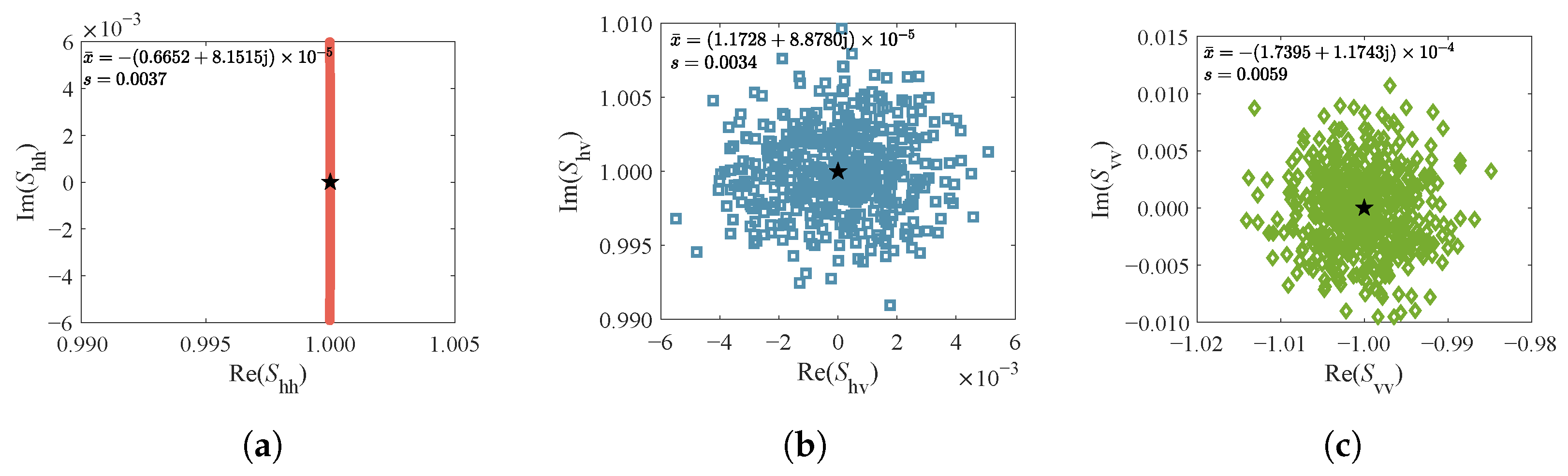
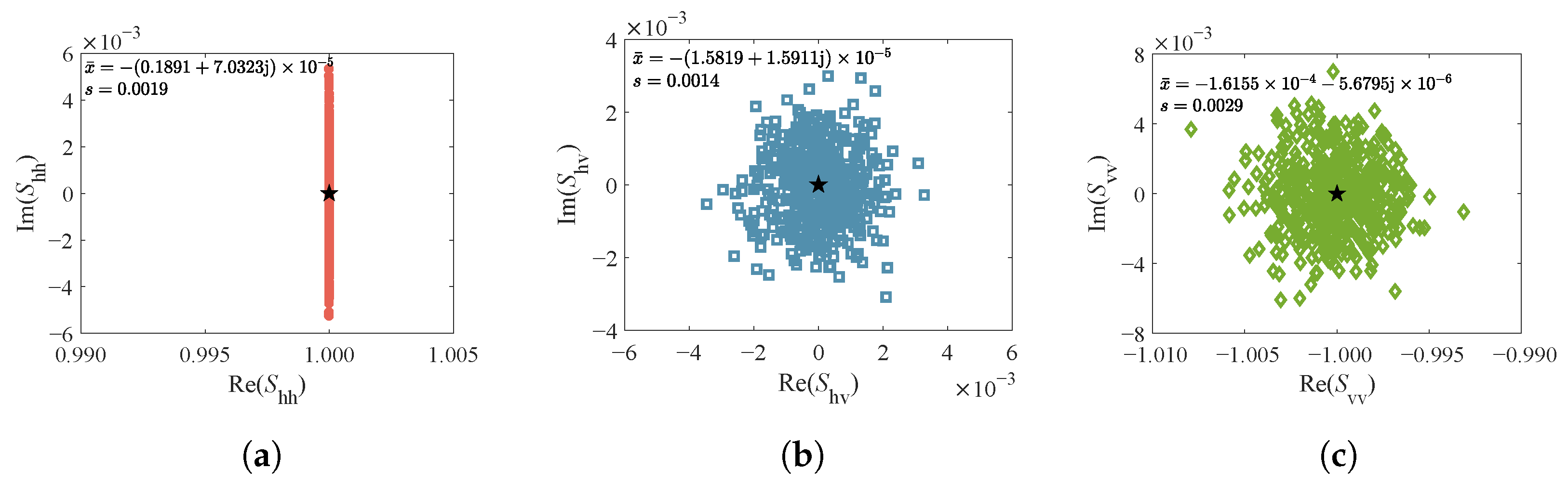
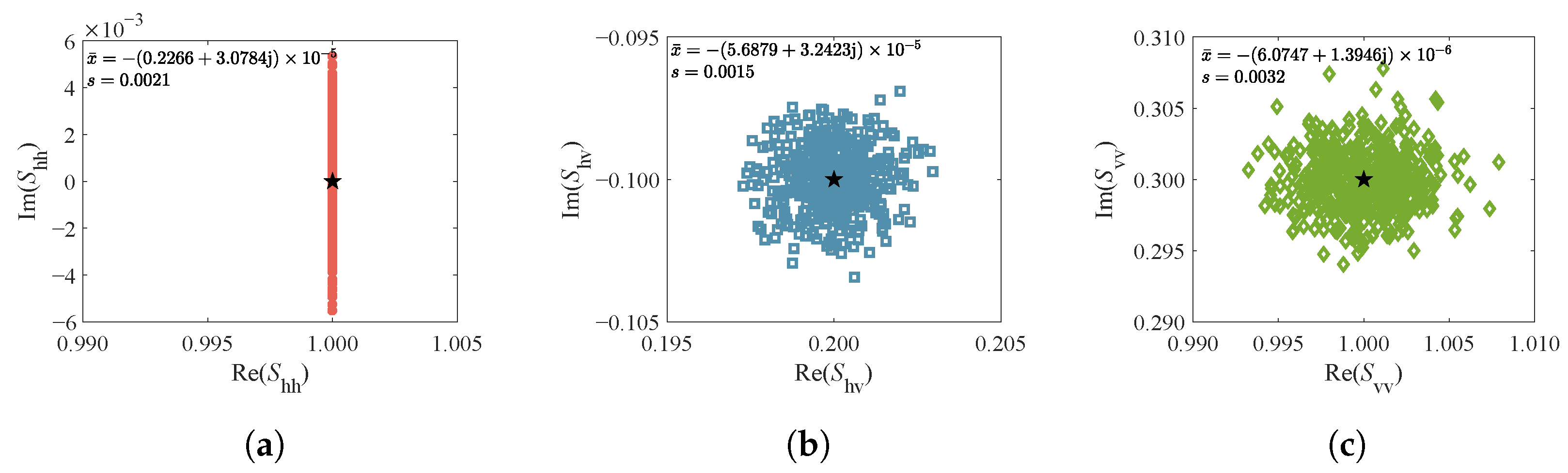
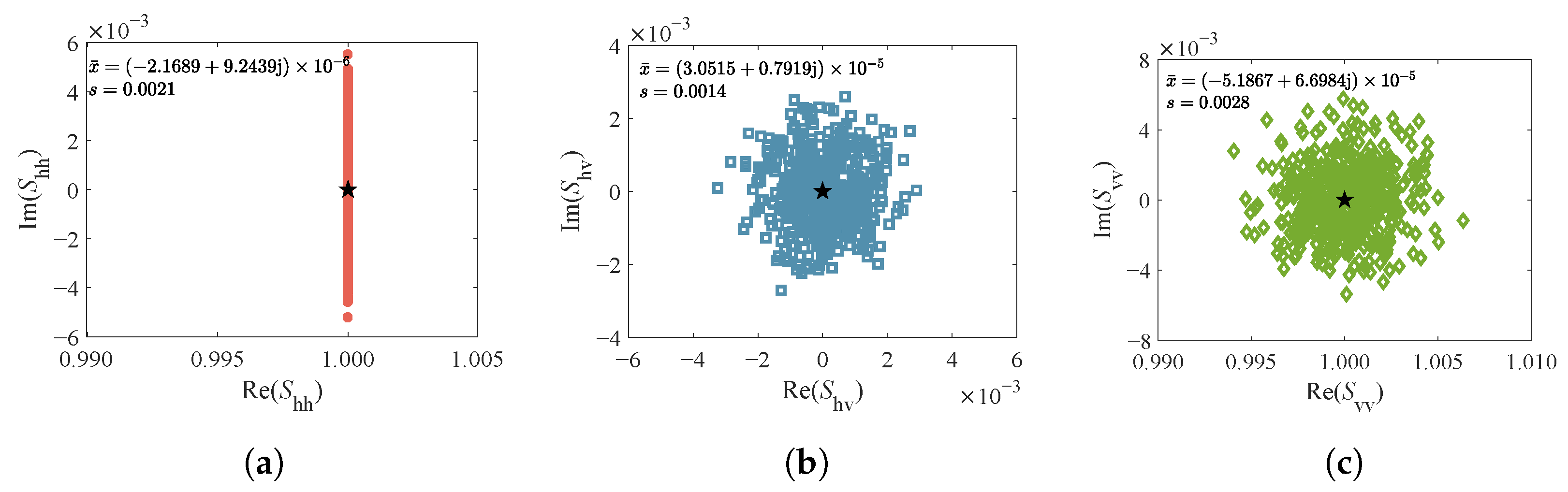
The PSM was estimated according to Equation (16). To ensure statistical reliability, 500 Monte Carlo simulation trials were conducted for each target. The complex-plane distribution of the estimated PSM values and the corresponding statistical errors for each target were analyzed (Figure 2, Figure 3, Figure 4 and Figure 5).

From the complex-plane distributions of the estimated PSM components, it can be observed that for the different targets, the mean estimation error of each PSM element is on the order of ${10}^{-5}$, and the mean square error (MSE) is on the order of ${10}^{-3}$. Combining this with Equations (21) and (22), it is concluded that the proposed algorithm achieves unbiased estimation for all four typical target types.

To assess estimation performance, the PSM estimation accuracy and Pauli decomposition accuracy were further analyzed using Equations (35) and (37), respectively, with the results reported in

Table 2. PSM estimation results and accuracy.

Target Type	True Value S	Estimated Value $\widehat{\mathbf{S}}$	${\mathit{e}}_{{\left|\mathit{a}\right|}^2}$	${\mathit{e}}_{{\left|\mathit{b}\right|}^2}$	${\mathit{e}}_{{\left|\mathit{c}\right|}^2}$	PSC
Left-handed helix structure	$\left[\begin{array}{cc}1& \mathrm{j}\\ \mathrm{j}& -1\end{array}\right]$	$\left[\begin{array}{cc}1-0.0001\mathrm{j}& 1.0001\mathrm{j}\\ 1.0001\mathrm{j}& -1.0002-0.0001\mathrm{j}\end{array}\right]$	$2.2\times {10}^{-5}$	$3.8\times {10}^{-3}$	$4.5\times {10}^{-3}$	1
Dihedral angle	$\left[\begin{array}{cc}1& 0\\ 0& -1\end{array}\right]$	$\left[\begin{array}{cc}1& 0\\ 0& -1.0002\end{array}\right]$	$4.0\times {10}^{-6}$	$1.6\times {10}^{-3}$	$4.1\times {10}^{-6}$	1
Standard metal ball	$\left[\begin{array}{cc}1& 0\\ 0& 1\end{array}\right]$	$\left[\begin{array}{cc}1& 0\\ 0& 0.9999+0.0001\mathrm{j}\end{array}\right]$	$3.2\times {10}^{-3}$	$4.0\times {10}^{-6}$	$3.9\times {10}^{-6}$	1
General scatterer	$\left[\begin{array}{cc}1& 0.2-0.1\mathrm{j}\\ 0.2-0.1\mathrm{j}& 1+0.3\mathrm{j}\end{array}\right]$	$\left[\begin{array}{cc}1& 0.1999-0.1\mathrm{j}\\ 0.1999-0.1\mathrm{j}& 1+0.3\mathrm{j}\end{array}\right]$	$1.9\times {10}^{-3}$	$1\times {10}^{-3}$	$7.2\times {10}^{-3}$	1

.

In Table 2, in addition to simple canonical targets, a “general scatterer” is introduced to represent a complex target. Unlike standard targets with specific structural symmetries, the true PSM elements of this general scatterer are arbitrarily chosen and deliberately exhibit asymmetric, random amplitudes and phases. The purpose of evaluating such an arbitrarily complex target is to firmly demonstrate the universal applicability of the proposed inversion algorithm, proving its capability to accurately reconstruct the full polarimetric information of generic targets without relying on any predefined symmetric properties.

As summarized in Table 2, the PSC values for all evaluated targets uniformly approach 1, indicating that the estimated PSMs closely match the true polarimetric scattering responses. In addition, the Pauli domain power errors are precisely controlled between ${10}^{-3}$ and ${10}^{-6}$, confirming that the estimator effectively preserves mechanism-indicative Pauli components while maintaining matrix-level accuracy. It is worth noting that these estimation accuracies are virtually identical across different targets because the proposed inversion is fundamentally based on solving a linear least squares system. Consequently, the estimation accuracy is inherently independent of the target’s specific scattering mechanism, exhibiting no bias toward any particular target type. The microscopic residual errors are purely attributed to the random fluctuations of system Gaussian white noise and the numerical limits of multi-pulse integration.

3.2. Robustness Analysis

3.2.1. Effects of SNR and Polarization Trajectory Geometry on PSM Estimation and Pauli Decomposition

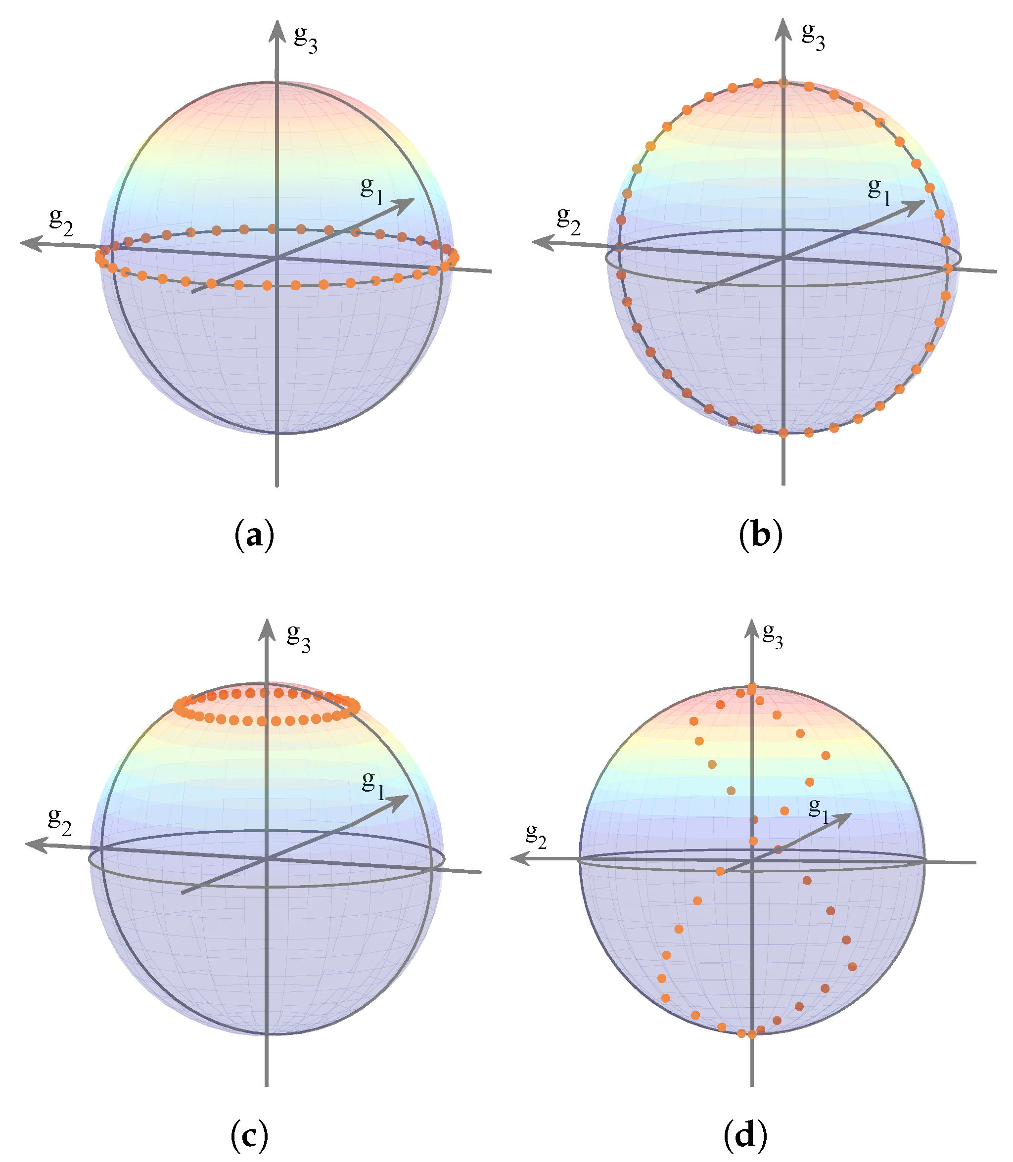
To investigate the impact of modulation-trajectory geometry, a polarization modulator was used to impose time-varying amplitude/phase modulation on the transmitted wave, yielding four representative Poincaré sphere trajectories:

(1)

Great-circle trajectory crossing the equator: The polarization phase remains constant along the trajectory, while the amplitude varies with time;

(2)

Great-circle longitudinal trajectory passing through 45° linear polarization: The amplitude ratio is fixed at unity along the trajectory, whereas the phase varies with time;

(3)

Small-circle trajectory parallel to the equator: Both the amplitude and phase evolve linearly with time at constant rates;

(4)

“8-like” trajectory: Both the phase difference and the amplitude ratio vary with time.

The corresponding trajectories on the Poincaré sphere are shown in Figure 6. In this experiment, all radar/target parameters follow Table 1, and only the trajectory geometry is adjusted.

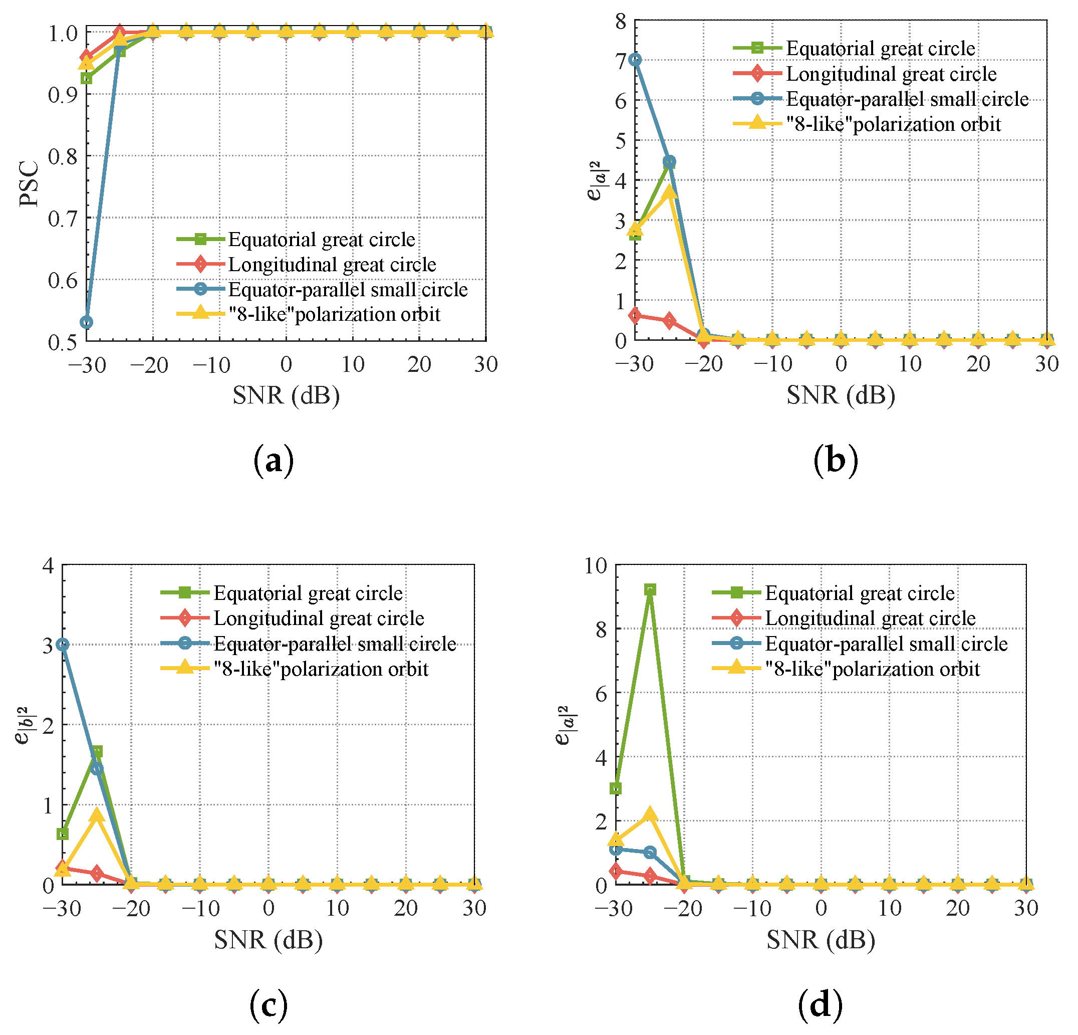
Based on the estimated $\widehat{\mathbf{S}}$, the dominant Pauli coefficients a, b, and c are computed. PSC quantifies the consistency between the estimated and true PSMs, and the relative errors of ${\left|a\right|}^2$, ${\left|b\right|}^2$, and ${\left|c\right|}^2$ characterize the ability of the estimator to preserve representative contributions from the scattering mechanism. The results are shown in Figure 7.

Figure 7a shows that when $\mathrm{SNR}\ge -20$ dB, the PSC values under all four trajectory constraints approach 1, indicating that the overall estimation accuracy of the scattering matrix is insensitive to the trajectory pattern. Consistently, the relative errors of the Pauli components in Figure 7b–d tend toward 0, demonstrating stable preservation of energy allocation between Pauli mechanism components. It should be noted that the reported SNR values refer to the pre-pulse-compression receiver input SNR. Considering the radar’s bandwidth and pulse width settings, matched filtering processing will provide approximately 20 dB of pulse compression gain.

When $\mathrm{SNR}<-20$ dB, performance degrades for all trajectories, but the degradation becomes strongly trajectory-dependent. For the small-circle trajectory parallel to the equator, PSC drops rapidly from 1 to 0.53 as SNR decreases from $-20$ to $-30$ dB, and the Pauli decomposition errors increase markedly, indicating a noise-dominated regime. In contrast, the two great-circle trajectories and the “8-like” trajectory maintain higher PSC (typically ≥0.93) and smaller Pauli decomposition errors at low SNR.

This behavior is mainly explained by polarization diversity and numerical conditioning: the small-circle trajectory spans a narrower set of polarization states in amplitude/phase, which reduces the effective rank of the observation equations. As noise increases, the pulse-compression peak becomes more susceptible to perturbations, degrading PSM estimation and destabilizing Pauli-component recovery.

In summary, for $\mathrm{SNR}\ge -20$ dB, all four trajectories support accurate PSM estimation, with PSC close to 1, and Pauli decomposition errors near zero. For $\mathrm{SNR}<-20$ dB, the small-circle trajectory is more sensitive to noise, whereas the two great-circle trajectories and the “8-like” trajectory exhibit superior robustness.

3.2.2. Impact of Polarimetric Diversity on PSM Estimation and Pauli Decomposition

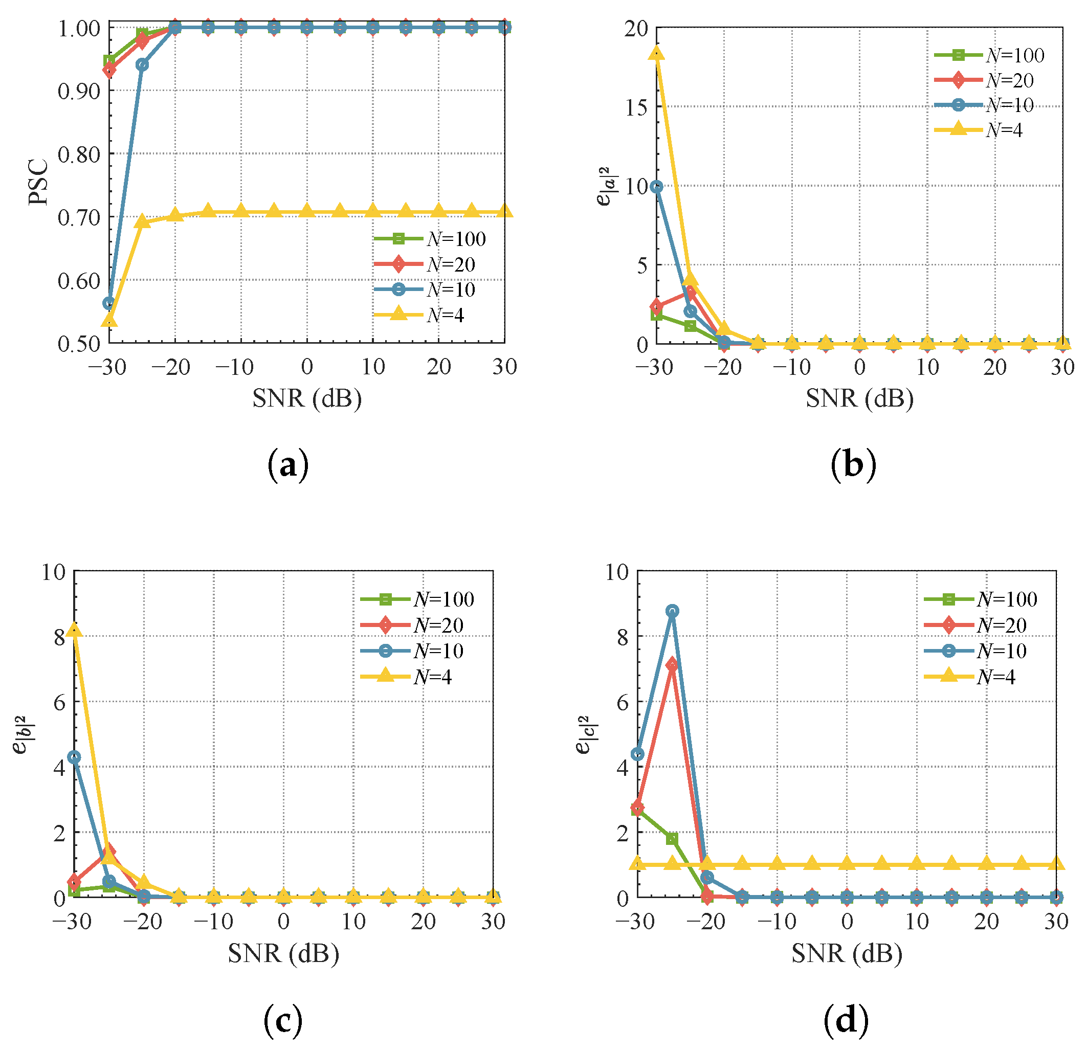
For inter-pulse polarization modulation, once the PRI of the radar signal is fixed, a longer modulation period yields more discretized polarization states and, hence, higher polarization diversity. Here, the number of polarization states per period is set to $N\in \{100,20,10,4\}$ to examine its impact on estimation performance.

Figure 8 shows that under low-SNR conditions (SNR $<-20$ dB), PSC degrades for all tested N and drops faster as N decreases. For $N\in \{100,20\}$, PSC decreases from 1 to about 0.94; for $N=10$, it decreases from 1 to about 0.66. When SNR exceeds $-20$ dB, the PSC for these cases approaches 1, indicating stable PSM estimation.

The Pauli decomposition errors follow the same trend as PSC. For SNR $<-20$ dB, the relative errors increase markedly; as SNR increases, they rapidly decrease and then stabilize near zero. Moreover, a larger N yields smaller errors overall.

Notably, when $N=4$, PSC remains below 0.72 and does not improve even at a high SNR. The Pauli decomposition results exhibit a persistent distortion, especially in the cross-polarization-related component derived from the off-diagonal terms of $\widehat{\mathbf{S}}$. This occurs because only four polarization states are available, resulting in an an insufficient rank for the polarization-modulation matrix.

It is important to note that the theoretical lower bound for solving the monostatic PSM is $N=3$ (Equations (12) and (13)). However, the performance of the proposed inversion algorithm is strictly governed by the singular value spectrum of the modulation matrix $\mathbf{P}$, which depends on the geometric relationship between the polarization orbit and the discrete sampling number N.

As shown in Figure 8, when $N=4$, the uniform sampling of the orbit results in a symmetric singularity (phase interval of $\pi /2$), causing the third singular value ${\sigma }_3$ to approach zero. Since our algorithm relies on a truncated singular value decomposition (TSVD) using the three largest singular values, this “symmetry trap” leads to a rank-deficient matrix approaching infinite and unstable inversion.

Increasing the number of pulses serves to optimize the condition number of matrix $\mathbf{P}$. A denser sampling along the orbit breaks the geometric symmetry, significantly increasing the minimal singular value ${\sigma }_3$ and stabilizing the solution against thermal noise. This analysis also suggests that future work could focus on polarization orbit optimization—designing trajectories that maximize ${\sigma }_3$ with minimal N—to further improve the temporal resolution of the system.

3.2.3. Doppler Mismatch on PSM Estimation and Pauli Decomposition

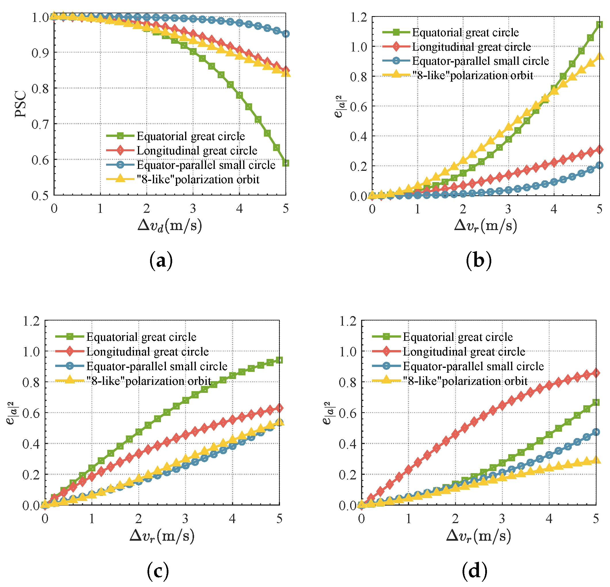
The preceding analyses assumed either a stationary target or an accurately known radial velocity. In this subsection, we examine the robustness of the proposed method under radial-velocity estimation errors, which are equivalent to Doppler-compensation mismatches. In the simulations, the velocity error was set as $\mathsf{\Delta }{V}_d\in [0,5]$ m/s, while the polarization states evolve along the four trajectories in Figure 6.

Figure 9a shows that PSC decreases monotonically as $\mathsf{\Delta }{V}_d$ increases, and the sensitivity is trajectory-dependent. The equator-parallel small-circle trajectory is the most tolerant, yielding PSC $>0.96$ even at $\mathsf{\Delta }{V}_d=5$ m/s. The longitudinal great-circle and the “8-like” trajectories are moderately robust, maintaining PSC $>0.9$ for $\mathsf{\Delta }{V}_d\le 4$ m/s. The equator-crossing great-circle trajectory is the most sensitive, requiring $\mathsf{\Delta }{V}_d\le 3$ m/s to keep the PSC above 0.9.

Consistent with the PSC, the relative errors of $|\widehat{a}{|}^2$, $|\widehat{b}{|}^2$, and $|\widehat{c}{|}^2$ increase with $\mathsf{\Delta }{V}_d$. The robustness ordering across trajectories matches that observed in PSC, although the absolute error magnitudes differ between the three components depending on the target scattering characteristics.

These results are explained by the residual inter-pulse phase error introduced by velocity mismatch. The residual phase yields a model mismatch between the pulse-compression peak vector and the assumed polarization modulation matrix, producing a systematic bias in $\widehat{\mathbf{S}}$ that propagates to the Pauli coefficients. The trajectory dependence reflects the different conditioning of the resulting least squares problem. In practice, robustness can be improved by optimizing the polarimetric trajectory and enhancing radial-velocity estimation accuracy.

It should be noted that the velocity error range of 3–5 m/s investigated here represents a conservative stress test. For a C-band SAR system ($f_c=5.3$ GHz), this corresponds to a Doppler frequency offset of 106–177 Hz. In modern spaceborne SAR missions, the Doppler Centroid frequency can typically be estimated with an accuracy within 5–30 Hz [53]. By testing the algorithm under error magnitudes nearly 50 times the industry standard, we demonstrate the extreme robustness of the proposed framework. In practical operational scenarios, the residual bias induced by Doppler mismatch is expected to be significantly lower, ensuring high-fidelity PSM retrieval.

3.2.4. Impact of Polarization Modulation Errors on PSM Estimation

In practice, polarization modulators have finite control accuracy, so the realized transmit/receive polarization states deviate from the commanded ones. Such modulation errors perturb the realized trajectory and introduce a model mismatch between the practical polarization modulation matrix and the ideal model used in the matched filtering and estimation stage.

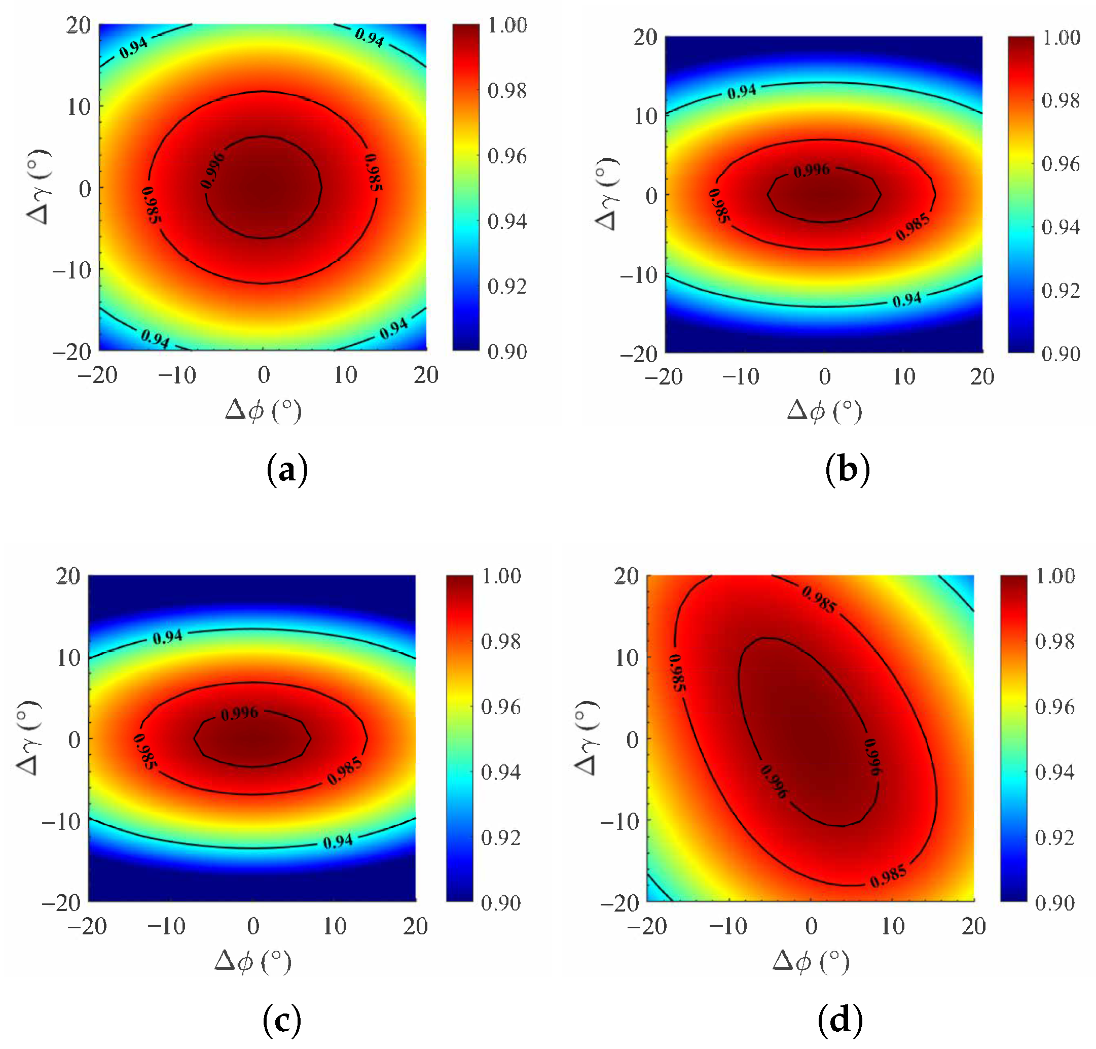
Accordingly, modulation errors are independently set as $\mathsf{\Delta }\gamma \in [-{20}^{\circ },{20}^{\circ }]$ and $\mathsf{\Delta }\varphi \in [-{20}^{\circ },{20}^{\circ }]$ with a step of $2^{\circ }$. The four trajectories in Figure 6 are examined with a common modulation frequency $f_m=500$ Hz and SNR $=20$ dB. The resulting PSC distributions versus $(\mathsf{\Delta }\gamma ,\mathsf{\Delta }\varphi )$ are shown in Figure 10.

As shown in Figure 10, the sensitivity to polarization modulation errors differs markedly across trajectory geometries. The “8-like” trajectory exhibits the best robustness, followed by the equatorial great-circle trajectory, whereas the longitudinal great-circle trajectory and the small-circle trajectory parallel to the equator are relatively more sensitive. It should be noted that the relative errors of the squared magnitudes of the three Pauli components are propagated from the scattering matrix estimation error. Therefore, their variation with $(\mathsf{\Delta }\gamma ,\mathsf{\Delta }\varphi )$ is broadly consistent with the PSC distribution. Regions with a higher PSC correspond to smaller overall errors of the three components, while deviations from the high-PSC region lead to a concurrent increase in all three component errors. Since the focus of this section is to provide accuracy tolerances and assess engineering feasibility for polarization modulation devices, the PSC is used hereafter as a representative metric for tolerance analysis.

For convenient back-calculation of device specifications, the PSC isolines at $\mathrm{PSC}=0.996$ and $\mathrm{PSC}=0.985$ are used as thresholds for high-accuracy and usable-accuracy, respectively. The corresponding allowable modulation-error regions under the four trajectories can be read from the isolines, yielding the following requirements:

(a)

Equatorial great-circle trajectory: To achieve $\mathrm{PSC}>0.996$, the errors should lie within an ellipse with a major-axis radius (along $\mathsf{\Delta }\varphi$) of $7^{\circ }$ and a minor-axis radius (along $\mathsf{\Delta }\gamma$) of $6^{\circ }$. To achieve $\mathrm{PSC}>0.985$, the errors should be confined within an ellipse with a major-axis radius (along $\mathsf{\Delta }\varphi$) of ${14}^{\circ }$ and a minor-axis radius (along $\mathsf{\Delta }\gamma$) of ${12}^{\circ }$.

(b)

Longitudinal great-circle polarization trajectory: To achieve $\mathrm{PSC}>0.996$, the errors should lie within an ellipse with a major-axis radius (along $\mathsf{\Delta }\varphi$) of $7^{\circ }$ and a minor-axis radius (along $\mathsf{\Delta }\gamma$) of $2.3^{\circ }$. To achieve $\mathrm{PSC}>0.985$, the errors should be confined within an ellipse with a major-axis radius (along $\mathsf{\Delta }\varphi$) of ${14}^{\circ }$ and a minor-axis radius (along $\mathsf{\Delta }\gamma$) of $7.3^{\circ }$.

(c)

Small-circle polarization trajectory with ${\gamma }_0=\pi /6$: To achieve $\mathrm{PSC}>0.996$, the errors should lie within an ellipse with a major-axis radius (along $\mathsf{\Delta }\varphi$) of $6.6^{\circ }$ and a minor-axis radius (along $\mathsf{\Delta }\gamma$) of $2.3^{\circ }$. To achieve $\mathrm{PSC}>0.985$, the errors should be confined within an ellipse with a major-axis radius (along $\mathsf{\Delta }\varphi$) of ${14}^{\circ }$ and a minor-axis radius (along $\mathsf{\Delta }\gamma$) of $6^{\circ }$.

(d)

“8-like” polarization trajectory: To achieve $\mathrm{PSC}>0.996$, the errors should lie within an ellipse whose major-axis radius is $11.6^{\circ }$ (along the diagonal direction in the plane spanned by $\mathsf{\Delta }\varphi$ and $\mathsf{\Delta }\gamma$) and whose minor-axis radius (along $\mathsf{\Delta }\gamma$) is $3.6^{\circ }$. To achieve $\mathrm{PSC}>0.985$, the errors should be confined within an ellipse with a major-axis radius (along $\mathsf{\Delta }\varphi$) of ${20}^{\circ }$ and a minor-axis radius (along $\mathsf{\Delta }\gamma$) of ${13}^{\circ }$.

In summary, the PSM estimation performance across different polarization trajectories, along with the associated tolerance requirements for polarization modulation errors, provides quantitative guidance for the design of polarization modulation device control accuracy.

3.3. Performance on Distributed Targets

In practical remote sensing applications, natural scenes, such as vegetation, are considered distributed targets. They are characterized by strong depolarization effects and random speckle textures, which are typically modeled using a full-rank polarimetric covariance matrix. To verify that the proposed Low-Rank Approximation (LRA) algorithm only suppresses additive thermal noise without accidentally filtering out the inherent texture/randomness of natural scattering, a Monte Carlo simulation involving vegetation clutter was conducted.

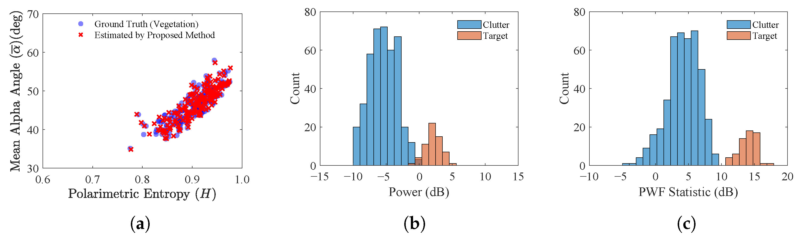
We simulated 500 independent samples of a vegetation canopy based on a multivariate complex Gaussian distribution. Cloude–Pottier eigenvalue decomposition was applied to analyze the statistical preservation. As shown in Figure 11a, the distribution of the estimated targets in the H-$\alpha$ plane aligns perfectly with the ground truth. Quantitatively, the estimated polarimetric entropy (H) and mean alpha angle ($\overline{\alpha }$) are 0.9066 and 46.5217°, respectively, which accurately match the true values ($H=0.9060$, $\overline{\alpha }=46.{4563}^{\circ }$). Furthermore, Figure 11b demonstrates that the proposed method accurately tracks the severe 1D spatial fluctuations of the vegetation clutter. These results rigorously prove that the LRA operation, which acts on the deterministic modulation matrix rather than the spatial covariance matrix, preserves the high-entropy physical nature of distributed targets without degrading them into deterministic point targets.

In addition to texture preservation, the ability to separate target PSM from heavy background clutter is crucial for low Signal-to-Clutter Ratio (SCR) scenarios. While the radar’s spatial resolution constrains physical decoupling within a single resolution cell, the proposed method provides a solid data foundation for polarimetric statistical separation.

To demonstrate this, a weak target embedded in heavy vegetation clutter was simulated. As illustrated in the histogram in Figure 11b, when using conventional single-channel power, the target energy is completely overlapped with the clutter distribution, making detection unfeasible. However, by accurately reconstructing the full equivalent PSM using the proposed method, mature PolSAR algorithms, such as the polarimetric whitening filter (PWF), can be directly applied. Since the artificial target and natural vegetation possess distinct polarimetric scattering mechanisms, the PWF effectively suppresses the clutter background. As shown in Figure 11c, the target and clutter distributions become clearly separated after processing. This confirms that the proposed single-channel modulation framework empowers resource-constrained platforms with advanced PolSAR target–clutter separation capabilities.

3.4. Compatibility with 2D SAR Azimuth Compression and PolSAR Imaging

While the primary focus of this paper and its numerical simulations is the 1D pulse-echo retrieval of the PSM for isolated point targets, it is imperative to clarify the compatibility of the proposed continuous pulse-to-pulse modulation ($P_n$) with standard 2D SAR azimuth focusing algorithms (e.g., range doppler algorithm (RDA) or chirp scaling algorithm (CSA)).

In a conventional SAR processing pipeline, azimuth focusing relies on the coherent integration of the Doppler phase. Uncompensated pulse-to-pulse modulation $P_n$ acts as an azimuth amplitude and phase weighting. Directly feeding these modulated raw echoes into RDA or CSA would severely corrupt the Doppler phase history, inevitably leading to grating lobes and degraded peak sidelobe ratios (PSLRs) and integrated sidelobe ratios (ISLRs).

To resolve this and achieve single-channel PolSAR imaging, the proposed PSM estimation framework (Equations (12)–(16)) acts as a polarimetric decoding and compensation module, implemented after range compression but before the azimuth Fourier transform.

Note that while the validation in Section 3 utilizes the peak of the range-compressed signal for a point target, this linear inversion framework is naturally extendable to 2D distributed scenes. Specifically, a sliding window of length N is applied along the azimuth slow-time. For each processing step, the inversion in Equation (13) is applied independently and in parallel across each range bin (range-bin-by-range-bin processing).

Through this localized slow-time inversion, the modulation $P_n$ is mathematically stripped off. Consequently, the single-channel modulated 2D data matrix is continuously reconstructed into four independent, unmodulated polarimetric 2D matrices (HH, HV, VH, and VV). For a given target, the reconstructed signal in each polarimetric channel perfectly restores its continuous, natural quadratic Doppler phase history along the azimuth slow-time $\eta$, which can be expressed as

$$S\left(\eta \right)\approx A_0·{\mathrm{e}}^{(-\mathrm{j}\frac{4\pi R\left(\eta \right)}{\lambda })}$$

(38)

where $\eta$ is the slow-time, $R\left(\eta \right)$ is the instantaneous range between the radar and the target, and $A_0$ is the true complex backscattering coefficient of the target. Because the modulation weighting $P_n$ is completely decoupled before the signal enters the Doppler frequency domain, the Point Spread Function (PSF) of the reconstructed signal remains theoretically identical to that of an unmodulated standard SAR system. However, since N pulses are consumed to retrieve one full PSM vector, the effective azimuth sampling rate is reduced to PRF_eq = PRF/N (pulse repetition frequency (PRF)).

To prevent azimuth aliasing, which would manifest as severe ghost targets and a drastically degraded ISLR, the radar system must be designed with an oversampling factor of at least N. In other words, the raw pulse repetition frequency must strictly satisfy PRF $\ge N·B_d$, where $B_d$ is the Doppler bandwidth of the target scene. This represents a fundamental engineering trade-off of the proposed framework; it trades a higher initial PRF (and, consequently, a higher raw data rate) for the significant hardware simplicity of a single-channel receiver.

Provided this oversampling criterion is met, when these compensated sequences are subsequently processed by standard range cell migration correction (RCMC) and azimuth compression algorithms, the theoretical azimuth resolution, PSLR, and ISLR of the focused PolSAR images will remain consistent with those of a conventional full polarimetric SAR system.

4. Discussion

The proposed framework successfully retrieves the full polarimetric scattering matrix (PSM) from single-channel echoes via time-varying polarization modulation. By solving an overdetermined linear system with a low-rank approximation, high-fidelity polarimetric information is recovered. Simulations confirm that the estimated PSMs maintain high similarity to the ground truth (near 1) and negligible Pauli decomposition errors (${10}^{-3}$∼${10}^{-6}$).

4.1. Robustness and Trajectory Dependence

Robustness analyses reveal a strong dependence on polarization trajectory geometry and measurement parameters. Reliable estimation requires an SNR $\ge -20$ dB and sufficient polarization diversity (e.g., $N\ge 10$ pulses per sequence) to ensure a well-conditioned modulation matrix. Conversely, under-sampling (e.g., $N=4$) or closely spaced states (e.g., the small-circle trajectory) reduces the effective rank of the observation equations, leading to persistent distortion. Furthermore, systematic biases induced by Doppler mismatch and modulation errors exhibit trajectory-specific sensitivities. For instance, the “8-like” trajectory demonstrates superior robustness against modulation errors, whereas the small-circle trajectory is more tolerant to radial–velocity mismatches. These findings highlight the necessity of trajectory optimization for practical applications.

4.2. Comparison with Compact Polarimetry (CP)

When evaluating resource-constrained PolSAR, the fundamental engineering trade-offs of the proposed method become evident compared with existing compact polarimetry (CP) architectures. While CP reduces transmitter complexity, it fundamentally requires simultaneous dual-channel reception, retaining the heavy hardware burden of two complete RF chains (typically including the low-noise amplifiers (LNAs), down-conversion chains, and ADCs, and doubled data rates. Moreover, reconstructing pseudo-quad-pol information from CP relies on strict physical and statistical priors, which frequently fail in heterogeneous urban scenes. In contrast, the proposed architecture operates with a strictly single receiver chain. By jointly inverting N modulated pulses, it deterministically recovers the exact full PSM without prior assumptions or spatial resolution degradation. The fundamental trade-off is exchanging the azimuth temporal sampling rate (necessitating an oversampled PRF) for ultimate baseband hardware simplicity (reduced SWaP-C) and assumption-free polarimetric fidelity.

4.3. Hardware Feasibility

To practically implement this pulse-to-pulse modulation within a single-channel RF frontend, specific hardware choices depend on system power limits. High-power spaceborne SAR can utilize fast ferrite polarization switches, while compact platforms (e.g., UAVs, CubeSats) may employ PIN-diode-loaded Reconfigurable Metasurface Antennas (RMAs). Since modern ferrite or diode switches transition within nanoseconds to a few microseconds, they can operate seamlessly within the typical SAR pulse repetition interval (PRI) dead time (tens of microseconds) without interfering with the pulse envelope. Because the architecture preserves a single coherent RF chain, all pulses share the same oscillator and receiver path, ensuring inherent phase stability across pulse-to-pulse polarization transitions. The modulation sequence is deterministically synchronized with the PRF, and therefore does not require additional inter-channel phase calibration beyond standard system calibration procedures. Although the frontend modulator introduces a slight insertion loss (typically 1–2 dB), it eliminates the substantial SWaP-C penalties of duplicating the baseband receiver.

4.4. Limitations and Future Work

A primary assumption of the current framework is that the target’s scattering properties remain constant during one modulation period (approximately 2 ms based on our parameters). While valid for static or macroscopically moving targets, highly dynamic environments (e.g., ocean surfaces) may introduce severe temporal decorrelation. Future work will investigate the impact of such rapid decorrelation on estimation accuracy and explore corresponding compensation strategies. Additionally, optimizing trajectory geometry and polarization encoding will be further pursued to maximize the system’s robustness against measurement mismatches.

5. Conclusions

A single-channel method for PSM estimation is presented, where time-varying polarization modulation is used to inject polarization diversity into single-channel echoes. With the resulting observation model, the PSM is recovered via a least squares formulation coupled with a low-rank approximation, enabling full polarimetric scattering information to be reconstructed on resource-constrained platforms while maintaining a single RF chain architecture augmented by a polarization modulator.

Simulation analysis illustrates high-precision PSM estimation for different targets. For random point targets, the matrix similarity approaches 1 and Pauli decomposition errors converge toward zero (reaching the ${10}^{-3}$ level) when the SNR exceeds $-20$ dB. Furthermore, the method’s reliability is validated on distributed vegetation clutter, where quantitative metrics demonstrate near-perfect statistical preservation, with polarimetric entropy and alpha angle errors within 0.14%. The estimation performance is robust even at SNR = $-20$ dB across different time-varying trajectories, confirming the feasibility of the approach for downstream analysis in complex natural scenes. Beyond feasibility, the key factors that govern reliability are clarified and translated into actionable design rules. It is shown that estimation performance is jointly determined by trajectory geometry, polarization diversity, and practical mismatches.

Building on these findings, future work will focus on the following three aspects: (i) the joint optimization of trajectory geometry and polarization diversity should be carried out under hardware constraints, improving algorithmic robustness while easing the difficulty of polarization modulation; (ii) improving estimation performance under non-ideal conditions (e.g., velocity-compensation errors and polarization-control errors) through joint estimation and calibration; and (iii) validation will be performed on measured data in increasingly complex scenes, where systematic error sources (e.g., antenna-pattern effects and channel imbalance) will be quantified and incorporated into the model.

References

1. Mott, H. Polarization in Antennas and Radar; Wiley-Interscience: New York, NY, USA, 1986. [Google Scholar]
2. Sinclair, G. The transmission and reception of elliptically polarized waves. Proc. IRE 1950, 38, 148–151. [Google Scholar] [CrossRef] [Scilit]
3. Gao, G.; Zhang, C.; Zhang, L.; Duan, D. Scattering characteristic-aware fully polarized SAR ship detection network based on a four component decomposition model. IEEE Trans. Geosci. Remote Sens. 2023, 61, 5222722. [Google Scholar] [CrossRef] [Scilit]
4. Li, H.L.; Liu, S.W.; Chen, S.W. PolSAR ship characterization and robust detection at different grazing angles with polarimetric roll-invariant features. IEEE Trans. Geosci. Remote Sens. 2024, 62, 5225818. [Google Scholar] [CrossRef] [Scilit]
5. Hurtado, M.; Xiao, J.J.; Nehorai, A. Target estimation, detection, and tracking. IEEE Signal Process. Mag. 2009, 26, 42–52. [Google Scholar] [CrossRef] [Scilit]
6. Zhao, Z.; Wen, Z.; Xue, C.; Cui, Z.; Hou, X.; Zhu, H.; Mu, Y.; Liu, Z.; Xia, Z.; Liu, X. Improved clutter suppression and detection of moving target with a fully polarimetric radar. Remote Sens. 2025, 17, 2975. [Google Scholar] [CrossRef] [Scilit]
7. Chen, S.W.; Li, M.D.; Cui, X.C.; Li, H.L. Polarimetric roll-invariant features and applications for polarimetric synthetic aperture radar ship detection: A comprehensive summary and investigation. IEEE Geosci. Remote Sens. Mag. 2024, 1, 36–66. [Google Scholar] [CrossRef] [Scilit]
8. Zhang, T.; Wang, W.; Quan, S.; Yang, H.; Xiong, H.; Zhang, Z.; Yu, W. Region-based polarimetric covariance difference matrix for polSAR ship detection. IEEE Trans. Geosci. Remote Sens. 2022, 60, 5222016. [Google Scholar]
9. Liu, Y.; Yang, P.; Liao, J. Investigation of target classification technology based on echo polarization characteristics. Opt. Laser Technol. 2025, 187, 112796. [Google Scholar] [CrossRef] [Scilit]
10. Hua, W.; Hou, Q.; Jin, X.; Liu, L.; Sun, N.; Meng, Z. A feature fusion network for PolSAR image classification based on physical features and deep features. IEEE Geosci. Remote Sens. Lett. 2024, 21, 4012705. [Google Scholar] [CrossRef] [Scilit]
11. Guo, Z.; Liu, Z.; Xie, R.; Ran, L. HRRP few-shot target recognition for full polarimetric radars via SCs optimal matching. IEEE Trans. Aerosp. Electron. Syst. 2025, 2, 4526–4541. [Google Scholar] [CrossRef] [Scilit]
12. He, Y.; Zhang, T.; He, H.; Zhang, P.; Yang, J. Polarization anti-jamming interference analysis with pulse accumulation. IEEE Trans. Signal Process. 2022, 70, 4772–4787. [Google Scholar] [CrossRef] [Scilit]
13. Zong, Z.W.; Shi, L.F.; Li, Y.; Wang, X.S. Detection-discrimination method for multiple repeater false targets based on radar polarization echoes. Radioengineering 2014, 23, 104–110. [Google Scholar]
14. Shi, L.F.; Wang, X.S.; Xiao, S.P. Polarization discrimination between repeater false-target and radar target. Sci. China Inf. Sci. 2009, 25, 149–158. [Google Scholar] [CrossRef] [Scilit]
15. Chen, S.; Wang, X.; Sato, M. Urban damage level mapping based on scattering mechanism investigation using fully polarimetric SAR data for the 3.11 east Japan earthquake. IEEE Trans. Geosci. Remote Sens. 2016, 54, 6919–6929. [Google Scholar] [CrossRef] [Scilit]
16. Margarit, G.; Mallorqui, J.J.; Fortuny-Guasch, J.; Lopez-Martinez, C. Exploitation of ship scattering in polarimetric SAR for an improved classification under high clutter conditions. IEEE Trans. Geosci. Remote Sens. 2009, 47, 1224–1235. [Google Scholar] [CrossRef] [Scilit]
17. Wang, N.; Jin, W.; Bi, H.; Xu, C.; Gao, J. A survey on deep learning for few-shot polSAR image classification. Remote Sens. 2024, 16, 4632. [Google Scholar] [CrossRef] [Scilit]
18. Zhang, S.; Cui, L.; Dong, Z.; An, W. A deep learning classification scheme for polSAR image based on polarimetric features. Remote Sens. 2024, 16, 1676. [Google Scholar] [CrossRef] [Scilit]
19. Karachristos, K.; Koukiou, G.; Anastassopoulos, V. A review on polSAR decompositions for feature extraction. J. Imaging 2024, 10, 75. [Google Scholar] [CrossRef] [Scilit]
20. Li, H.Z.; Wang, C.; Zhang, H.; Liu, L. A unified three-component scattering model for polarimetric coherent target decomposition. Int. J. Remote Sens. 2012, 33, 2868–2891. [Google Scholar] [CrossRef] [Scilit]
21. Chen, Z.; Xu, Z.; Ai, X.; Wu, Q.; Liu, X.; Cheng, J. A novel method for polISAR interpretation of space target structure based on component decomposition and coherent feature extraction. Remote Sens. 2025, 17, 1079. [Google Scholar] [CrossRef] [Scilit]
22. van Zyl, J. The effect of topography on radar scattering from vegetated areas. IEEE Trans. Geosci. Remote Sens. 1993, 31, 153–160. [Google Scholar] [CrossRef] [Scilit]
23. Huang, Z.; Gao, J.; Lv, X.; Li, X. Joint-pixel inversion for ground phase and forest height estimation using spaceborne polarimetric SAR interferometry. Remote Sens. 2025, 17, 1726. [Google Scholar] [CrossRef] [Scilit]
24. Chang, J.G.; Kraatz, S.; Oh, Y.; Gao, F.; Anderson, M. Quality assessment of dual-polarization C-band SAR data influenced by precipitation based on normalized polarimetric radar vegetation index. Remote Sens. 2025, 17, 2343. [Google Scholar] [CrossRef] [Scilit]
25. Liu, J.; Li, C.; He, X.; Chen, T.; Jia, X.; Bai, Y.; Liu, D.; Qu, B.; Wang, Y.; Feng, X.; et al. Impact of the uncertainties of polarized water-leaving radiance on the retrieval of oceanic constituents and inherent optical properties in global oceans via multiangle polarimetric observations. Remote Sens. 2025, 17, 1148. [Google Scholar] [CrossRef] [Scilit]
26. Taleghanidoozdoozan, S.; Xu, L.; Clausi, D.A. Region-based sea ice mapping using compact polarimetric synthetic aperture radar imagery with learned features and contextual information. Remote Sens. 2023, 15, 3199. [Google Scholar] [CrossRef] [Scilit]
27. Shu, S.; Yang, J.; Yang, C.; Hu, H.; Jing, W.; Hu, Y.; Li, Y. Performance analysis of ocean eddy detection and identification by L-band compact polarimetric synthetic aperture radar. Remote Sens. 2021, 13, 4905. [Google Scholar] [CrossRef] [Scilit]
28. Margarit, G.; Mallorqui, J.; Rius, J. On the usage of GRECOSAR, an orbital polarimetric SAR simulator of complex targets, to vessel classification studies(Article). IEEE Trans. Geosci. Remote Sens. 2006, 44, 3517–3525. [Google Scholar] [CrossRef] [Scilit]
29. Zhang, T.; Quan, S.; Yang, Z.; Guo, W.; Zhang, Z.; Gan, H. A two-stage method for ship detection using polSAR image. IEEE Trans. Geosci. Remote Sens. 2022, 60, 5236918. [Google Scholar] [CrossRef] [Scilit]
30. Wu, G.; Wang, S.L.; Liu, Y.; Wang, P.; Li, Y. Ship contour extraction from polarimetric SAR images based on polarization modulation. Remote Sens. 2024, 16, 3669. [Google Scholar] [CrossRef] [Scilit]
31. Wu, S.; Wang, W.; Deng, J.; Quan, S.; Ruan, F.; Guo, P.; Fan, H. Nearshore ship detection in polSAR images by integrating superpixel-level GP-PNF and refined polarimetric decomposition. Remote Sens. 2024, 16, 1095. [Google Scholar] [CrossRef] [Scilit]
32. Huynen, J. Measurement of the target scattering matrix. Proc. IEEE 1965, 53, 936–946. [Google Scholar] [CrossRef] [Scilit]
33. Kollias, P.; McLaughlin, D.J.; Frasier, S.; Oue, M.; Luke, E.; Sneddon, A. Advances and applications in low-power phased array X-band weather radars. In Proceedings of the 2018 IEEE Radar Conference (RadarConf18), Oklahoma City, OK, USA, 23–27 April 2018. [Google Scholar]
34. Chen, S.; Wang, X. Polarimetric synthetic aperture radar interpretation and recognition: Advances and perspectives. J. Radars 2020, 9, 259–276. [Google Scholar]
35. Raney, R.K. Hybrid-polarity SAR architecture. IEEE Trans. Geosci. Remote Sens. 2007, 45, 3397–3404. [Google Scholar] [CrossRef] [Scilit]
36. Thompson, A. Overview of the RADARSAT constellation mission. Can. J. Remote Sens. 2015, 41, 401–407. [Google Scholar] [CrossRef] [Scilit]
37. Goswami, J.N.; Annadurai, M. Chandrayaan-1: India’s first planetary science mission to the moon. Curr. Sci. 2009, 96, 486–491. [Google Scholar]
38. Giuli, D.; Fossi, M.; Facheris, L. Radar target scattering matrix measurement through orthogonal signals. IEE Proc. F Radar Signal Process. 1993, 140, 233–242. [Google Scholar] [CrossRef] [Scilit]
39. Fan, Y.; Chen, D.; Chen, S.; Su, J.; Tao, M.; Guo, Z.; Wang, L. Weak target detection based on full-polarization scattering features under sea clutter background. Remote Sens. 2024, 16, 2987. [Google Scholar] [CrossRef] [Scilit]
40. Nord, M.; Ainsworth, T.; Lee, J.; Stacy, N. Comparison of compact polarimetric synthetic aperture radar modes. IEEE Trans. Geosci. Remote Sens. 2009, 47, 174–188. [Google Scholar] [CrossRef] [Scilit]
41. Song, G.; Deng, Y.; Zhang, H.; Liu, X.; Chang, S. Improving SAR ship detection accuracy by optimizing polarization modes: A study of generalized compact polarimetry (GCP) performance. Remote Sens. 2025, 17, 1951. [Google Scholar] [CrossRef] [Scilit]
42. Zhang, Z.; Zhao, Z.; Qi, Y.; Xiong, M. Dual-polarization radar quantitative precipitation estimation (QPE): Principles, operations, and challenges. Remote Sens. 2025, 17, 3619. [Google Scholar] [CrossRef] [Scilit]
43. Ghods, S.; Vahab Shojaedini, S.; Maghsoudi, Y. A modified H-α classification method for DCP compact polarimetric mode by reconstructing quad H and α parameters from dual ones. IEEE J. Sel. Topics Appl. Earth Observ. Remote Sens. 2016, 9, 2233–2241. [Google Scholar] [CrossRef] [Scilit]
44. Chang, S.; Tang, S.; Deng, Y.; Zhang, H.; Liu, D.; Wang, W. An advanced scheme for deceptive jammer localization and suppression in elevation multichannel SAR for underdetermined scenarios. IEEE Trans. Aerosp. Electron. Syst. 2025, 1–18. [Google Scholar] [CrossRef] [Scilit]
45. Song, S.; Dai, Y.; Song, Y.; Jin, T. Efficient near-field radar microwave imaging based on joint constraints of low-rank and structured sparsity at low SNR. IEEE Trans. Microw. Theory 2025, 73, 2962–2977. [Google Scholar] [CrossRef] [Scilit]
46. Eriksson, A.; van den Hengel, A. Efficient computation of robust weighted low-rank matrix approximations using the L 1 Norm. IEEE Trans. Pattern Anal. Mach. Intell. 2012, 34, 1681–1690. [Google Scholar] [CrossRef] [Scilit]
47. Chen, Y.; Wang, Z.; An, M.; Wu, G.; Jiang, M.; Wang, Z.; Li, Y. A low-cost scattering matrix measurement method via single-channel polarization information. IEEE Antennas Wirel. Propag. Lett. 2025, 1–5. [Google Scholar] [CrossRef] [Scilit]
48. Li, Z. Design, Simulation and Validation of Dual-Channel Polarimetric Agile Radar Technology. Ph.D. Thesis, Delft University of Technology, Delft, The Netherlands, 2011. [Google Scholar]
49. Li, C.; Yang, Y.; Wang, X.S.; Li, Y. Moving target scattering matrix measurement using the three polarizations scheme. IEEE Geosci. Remote Sens. Lett. 2019, 16, 1555–1559. [Google Scholar] [CrossRef] [Scilit]
50. Ding, Y.; Liu, M.; Li, S.; Jia, D.; Zhou, L.; Wu, B.; Wang, Y. Mountainous landslide recognition based on Gaofen-3 polarimetric SAR imagery. In Proceedings of the IGARSS 2019, Yokohama, Japan, 28 July–2 August 2019; pp. 9634–9637. [Google Scholar]
51. Prajapati, K.; Prajapati, P.; Ramakrishnan, R.; Mahajan, A.; Bhavsar, M. Feature combination of Pauli and H/A/Alpha decomposition for improved oil spill detection using SAR. In Recent Trends in Image Processing and Pattern Recognition, Proceedings of the Third International Conference, RTIP2R 2020, Aurangabad, India, 3–4 January 2020; Springer: Singapore, 2021; pp. 134–147. [Google Scholar]
52. Ohki, M.; Abe, T.; Tadono, T.; Shimada, M. Landslide detection in mountainous forest areas using polarimetry and interferometric coherence. Earth Planets Space 2020, 72, 67. [Google Scholar] [CrossRef] [Scilit]
53. Renga, A.; Moccia, A. Use of Doppler parameters for ship velocity computation in SAR images. IEEE Trans. Geosci. Remote Sens. 2016, 54, 3995–4011. [Google Scholar] [CrossRef] [Scilit]
Figure 1. Overview of the proposed single-channel PSM estimation framework. (a) Single RF chain radar augmented with a polarization modulator. (b) Time-varying transmit/receive polarization states encode controllable polarization tags into the echoes through the target’s polarization-dependent response. (c) The signal processing block diagram of the proposed model, illustrating the step-by-step pipeline from pulse-compressed of the single-channel echoes to the final PSM inversion.
Remotesensing 18 00870 g001
Figure 2. The complex-plane distribution of the estimated PSM values of the left-handed helix structure ( S = 1 j ; j 1 ): (a) S hh ; (b) S hv ; (c) S vv . The pentagram marks the ground-truth position.
Remotesensing 18 00870 g002
Figure 3. The complex-plane distribution of the estimated PSM values of the dihedral angle structure ( S = 1 0 ; 0 1 ): (a) S hh ; (b) S hv ; (c) S vv . The pentagram marks the ground-truth position.
Remotesensing 18 00870 g003
Figure 4. The complex-plane distribution of the estimated PSM values of the standard metal ball ( S = 1 0 ; 0 1 ): (a) S hh ; (b) S hv ; (c) S vv . The pentagram marks the ground-truth position.
Remotesensing 18 00870 g004
Figure 5. The complex-plane distribution of the estimated PSM values of the general scatter ( S = 1 ,   0.2 0.1 j ; 0.2 0.1 j ,   1 + 0.3 j ): (a) S hh ; (b) S hv ; (c) S vv . The pentagram marks the ground-truth position.
Remotesensing 18 00870 g005
Figure 6. Four different polarization-agile trajectories. (a) Equatorial great-circle polarization trajectory. (b) Longitudinal great-circle polarization trajectory. (c) Small-circle polarization trajectory parallel to the equator. (d) “8-like” polarization trajectory.
Remotesensing 18 00870 g006
Figure 7. Robustness of the proposed method in terms of PSC and Pauli decomposition errors versus polarization-agile trajectories and SNRs: (a) polarization similarity coefficient; (b) relative error of | a | 2 ; (c) relative error of | b | 2 ; (d) relative error of | c | 2 .
Remotesensing 18 00870 g007
Figure 8. Robustness of the proposed method in terms of PSC and Pauli decomposition errors versus polarization-agile period length and SNR: (a) polarization similarity coefficient; (b) relative error of | a | 2 ; (c) relative error of | b | 2 ; (d) relative error of | c | 2 .
Remotesensing 18 00870 g008
Figure 9. Robustness of PSC and Pauli decomposition errors against velocity estimation errors: (a) polarization similarity coefficient; (b) relative error of | a | 2 ; (c) relative error of | b | 2 ; (d) relative error of | c | 2 .
Remotesensing 18 00870 g009
Figure 10. Robustness of polarimetric scattering information estimation performance to polarization modulation errors: (a) equatorial great-circle polarization trajectory; (b) longitudinal great-circle polarization trajectory; (c) small-circle polarization trajectory parallel to the equator; (d) “8-like” polarization trajectory.
Remotesensing 18 00870 g010
Figure 11. Simulation results of the proposed single-channel PSM estimation for distributed targets. (a) H- α plane characterizing the target scattering mechanisms; (b) Modulated single-channel echo power before processing; (c) Reconstructed power spatial distribution after the proposed processing.
Remotesensing 18 00870 g011