Article

Particle Size Characteristics at the Top of Biomass Burning Plumes Based on Two Case Studies

1
Faculty of Applied Sociology, Kindai University, Higashiosaka 577-8502, Japan
2
School of Applied Information Technology, The Kyoto College of Graduate Studies for Informatics, Kyoto 606-8225, Japan
3
CNRS (Centre National de la Recherche Scientifique), University of Lille, F-59000 Lille, France
*
Author to whom correspondence should be addressed.
Remote Sens. 2026, 18(5), 747; https://doi.org/10.3390/rs18050747
Submission received: 23 January 2026 / Revised: 25 February 2026 / Accepted: 27 February 2026 / Published: 1 March 2026
(This article belongs to the Special Issue Aerosol Remote Sensing from Space, Ground or Computers)

Highlights

What are the main findings?
  • By utilizing CGOM-C/SGLI data, we derived the plume top characteristics (geometric height, optical properties, or their relation) of biomass burning aerosols (BBA) due to large-scale wildfires.
  • It was found that BBA size decreases with plume altitude, and this finding was validated by SGLI polarization data and Radiative Transfer calculations.
What is the implication of the main finding?
  • By understanding the detailed characteristics at the top of the plume, it is possible to predict the advection and lifetime of the BBA plume.
  • The algorithm and results proposed in this study can be applied to the monitoring of aerosol disasters, including not only BBA plumes but also dust events, volcanic eruptions, and high-concentration PM pollution.

Abstract

Biomass burning aerosols (BBA) released from large-scale wildfires pose a serious threat worldwide, necessitating a comprehensive understanding of their plume characteristics. To address this challenge, this study used satellite data provided by the Second-generation Global Imager (SGLI) aboard the Global Change Observation Mission-C and regional-scale numerical chemical transport model (CTM) simulations to characterize BBA plumes. The SGLI data and CTM simulations were compared and verified, and the 3D characteristics of BBA plumes, including concentration, diffusion range, spatial variation in optical properties, plume top height, and vertical profile, were subsequently derived. In this study, we focused on large-scale forest fires that occurred in western North America in September 2020 and Indonesia in September 2019. In both cases, Aerosol optical thickness (AOT) and Ångström Exponent (AE) values show a positive correlation with the height of the BBA plume top. The results showed that the higher the BBA plume top, the thicker the plume and the smaller the aerosol size. This point is what we particularly wish to highlight in this study. The SGLI polarization data proved useful for characterizing the upper layers of the BBA plumes. By understanding the detailed characteristics at the top of the plume, it is possible to predict the BBA plume’s advection and lifetime.

1. Introduction

Large-scale wildfires have become a major global problem owing to the large amounts of biomass-burning aerosols (BBA) they release into the atmosphere. Wildfires occur in various regions worldwide, not only near the equator but also in higher latitudes, such as the USA, Canada, and Siberia. These severe fires are often caused by a combination of dryness, high temperatures, and strong winds [1]. In recent years, large-scale wildfires have frequently occurred during the dry season in western North America [2]. We have detected smoke from severe forest fires in this area using satellite data [3]. The forest fire outbreak occurring in the suburbs of Los Angeles, USA, at the beginning of 2025, underscores the severity of fire threats in a changing climate.
BBA emissions from wildfires have significant social and climatic consequences. BBAs cause long-range advection, migration, and air pollution, which pose significant health hazards [4,5,6]. High concentrations of BBAs in plumes can travel long distances, causing widespread air pollution. Even after dissipation, they have long-term global climate impacts through their direct and indirect radiative effects and persist in the atmosphere [7,8,9]. Large volcanic eruptions have effects similar to those of BBA plumes from wildfires [10,11]. In addition, dust storms are a serious global challenge. In East Asia, air pollution caused by fine particulate matter is another serious problem. Collectively, these are referred to as atmospheric particulate hazards. Ozone-related air pollution and its health impacts are also emerging as challenges [12].
The prediction of BBA plume advection and lifetime requires an estimation of the size and height of BBA plumes. Therefore, this study attempted to elucidate the 3D elements of BBA plumes. Specifically, BBA plume top height estimation was performed using a simple version of the stereoscopic method that was developed for the Multi-angle Imaging SpectroRadiometer (MISR) [13,14,15]. Multidirectional MISR data have been used to estimate the top heights of clouds and BBA plumes [13,16], and their advantages have been widely recognized [17,18]. A previous study has implemented the adapted version of the algorithm on the Second-generation Global Imager (SGLI) on board Global Change Observation Mission-C (GCOM-C) [19]. In the present study, as well, SGLI satellite data were used because of their advantageous features, such as a wide observation swath, near-ultraviolet spectral channels, and simultaneous multi-spectral and polarization observations. These characteristics serve as effective tools for BBA analysis.
An understanding of the meteorological field is necessary for capturing the long-range advection transport of BBA particles and air pollution. Numerical meteorological model simulations are useful for interpreting BBA behavior. In this study, a chemical transport model (CTM) [20,21] that utilizes meteorological fields simulated by Scalable Computing for Advanced Library and the Environment Regional Model (SCALE) [22,23] was employed for offline calculations. Notably, thermally driven flows are a feature of mountainous weather in certain regions [24,25]. Therefore, topographic effects and meteorological information are essential for understanding airflow, particularly in mountainous regions [21,26]. A regional CTM corresponding to detailed spatial scales can be effective for simulating such an atmosphere over complex terrain. BBA events, which form a characteristic plume, can trigger the formation of clouds, and the boundary between heavy aerosols and clouds is often ambiguous [27]. This is interesting from the perspective of atmospheric particle formation and elucidation of the generation and advection processes of BBA particles. The CTM can simulate spatiotemporal changes in the behavior of BBA plumes as they spread from the fire source into the atmosphere in accordance with the wind direction. Consequently, in this study, optical BBA properties were retrieved from SGLI data based on vector radiative transfer (RT) calculations in an optically thick atmospheric model [3,28]. The retrieved results were then validated using NASA/ The AErosol RObotic NETwork (AERONET) ground-based observational data and compared with 3D simulations to confirm the reliability of the CTM. Because GCOM-C is a polar-orbiting satellite with a return period of four days, complementary information, such as meteorological satellite data from the NASA/Geostationary Operational Environmental Satellite (GOES), was utilized to describe the time variation of wildfires.
This study positions itself as a first step toward linking the detection and analysis of disasters caused by atmospheric particles—such as massive volcanic eruptions, dust storms, and high-concentration air pollution particles—to prediction, not limited to smoke particles from large-scale wildfires. Understanding the dynamics of atmospheric particles, which exhibit significant spatial and temporal variability, requires the mutual utilization of numerical models and satellite and ground-based observations. Therefore, we also pay attention to considering numerical model input variables such as emission inventory from biomass burning [15,29,30] and implementing mutual verification between model simulations and observations at various stages and phases. The motivation of this study is to put in context the technical findings that are demonstrated for the GCOM-C/SGLI sensor in previous works [19,21,28,30,31] and to analyze the relationship between plume height and aerosol size, with a particular focus on plume top height—a critical parameter for disasters caused by atmospheric particles.

2. Materials and Methods

2.1. SGLI Observations

The GCOM-C/SGLI, which is the main resource used in this study, has 19 channels ranging from near-UV to thermal IR and includes red (674 nm; PL1 band) and near-IR (869 nm; PL2 band) polarization [32]. Table 1 summarizes the channel specifications for SGLI. The instantaneous field-of-view of the SGLI is 250 m in the near-UV to short-wave IR wavelength range and 1 km for polarization measurements. It is useful for atmospheric particle hazard studies because of its near-UV bands, polarization bands, high spatial resolution, and wide observation swath (1150 km in the visible to near-IR and 1400 km in the IR wavelengths). The SGLI was the only sensor mounted on the Japanese mission JAXA/GCOM-C (SHIKISAI in Japanese) launched in December 2017 and continues to provide Earth observation data beyond its designed life of five years.
Atmospheric particles (aerosols) are small, yet their size, composition, and even shape change over time and location. To detect these elusive, ever-changing aerosols, we must first roughly detect and classify them from satellite data. This is where SGLI’s near-UV data proves invaluable. Looking back in history, the Total Ozone Mapping Spectrometer (TOMS) aboard the Nimbus 7 satellite demonstrated that ultraviolet wavelengths are effective for aerosol remote sensing, particularly for absorbing aerosols such as carbonaceous aerosols and mineral dust. This is known as TOMS-AI (Aerosol Index) [33]. That is, the 380 and 412 nm channels are particularly useful for detecting absorbing particles, such as carbonaceous aerosols and mineral dust particles. The key index for the detection and classification, absorbing aerosol index (AAI), is calculated as follows:
AAI = R-ref (412)/R-ref (380).
The reflectance R-ref represents the observed satellite value. Note that the definition of our AAI is different from those employed by the TOMS in the formula and the reference channels. BBA-dominant areas have AAI values of ≥1.0 and ≥1.1, which suggest heavy and severe BBA events, respectively. In most large-scale fires, the AAI is ≥1.1, although this threshold is not a strict value. Note that mineral dust particles, another type of absorbing aerosol, do not have such high AAI values, making the use of the AAI index advantageous for detecting BBAs in large-scale wildfires.
The second BBA indicator employed in this study was the polarized radiance index (PRI). Polarization is described by the Stokes parameters I , Q , U , V , where the first element I represents the radiance of reflectance from the top of the atmosphere, and the remaining three elements represent the state of polarization. The PRI is defined using the polarized reflectance P-ref (λ) at wavelength λ, where the vector radiation field is defined as a ratio of polarized reflectance as in the following equations:
P - r e f ( λ ) = Q λ 2 + U λ 2
PRI = P-ref (869 nm)/P-ref (674 nm).
BBA plume exhibits values of PRI ≥ 1.2 and AAI ≥ 1.1. However, since the region where AAI ≥ 1.1 encompasses the region where PRI ≥ 1.2, only AAI ≥ 1.1 is used here as the BBA detection condition. Therefore, the AAI can be used to quickly determine severe BBA events [31], and the PRI is useful for polarization sensors that are not available for near-UV data. This technique demonstrated the rapid detection of BBA directly from satellite data by utilizing two types of wavelength ratio indices that leverage the characteristics of SGLI data. The BBA detection algorithm derived from SGLI observation data was validated using polarization reflectance calculated via radiative transfer simulation [34].
Subsequently, this study exploits the significant advantage of the SGLI polarization measurements. A spatial resolution of 1 km is the best among publicly available multiyear global-scale polarization measurement datasets. Although polarization information itself is useful for atmospheric particle and cloud analysis, the tilted measurement by the SGLI polarization channels offers, in addition, the opportunity of stereoscopy. Specifically, SGLI polarization measurements use a dedicated optical system mounted on a tilt mechanism. The tilt angle of the polarization optics is fixed at a forward 45° in the Northern Hemisphere and a backward 45° in the Southern Hemisphere. These tilted polarization optics enable global two-directional radiance measurements in combination with nadir multispectral radiance-only optics. As the SGLI moves from north to south on the day side of the orbit, a ground target in the Northern Hemisphere is first measured by forward-tilted polarization optics and approximately 2 min later by nadir radiance optics; the reverse order is used in the Southern Hemisphere. Figure 1 shows a schematic of SGLI two-directional data acquisition. Polarization optics views the 45° direction, although radiance optics has a straight-down view. Thus, two-directional radiance data are obtained at every SGLI pixel. By using this two-directional data, the BBA plume top height can be estimated. From the two-directional images, the 3D position of the target could be estimated by a method similar to triangulation. More precisely, the plume images acquired from two view directions present a shift when they are projected onto the Earth ellipsoid. The amount of shift that is detected by the Normalized Cross Correlation template matching tells the altitude of the plume. This study applies the method described in the previous work [19,31].

2.2. CTM Simulations

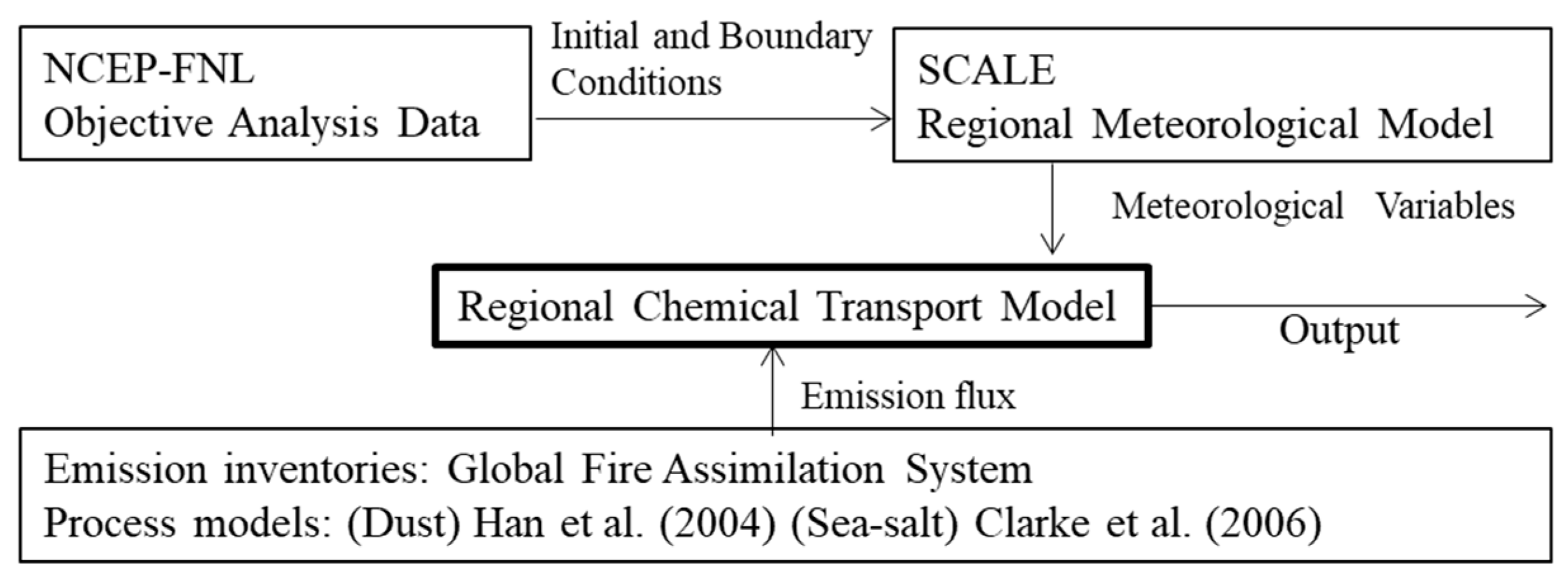
The CTM employed in this study [21] is based on the NHM-Chem chemical transport model [20], utilizing meteorological fields provided by the SCALE [22,23] model for offline calculations. Figure 2 shows an overview of the model configuration and input data used in this study. Operational global analysis data from the National Centers for Environmental Prediction were employed as the initial and boundary conditions of the SCALE. These products are provided by the Global Data Assimilation System, which continuously collects observational data through the World Meteorological Organization’s Global Telecommunications System and from other sources. SCALE reads and stores atmospheric state input data as predictive variables, then calculates time evolution by invoking various components such as the dynamic core and physical processes. Offline CTM calculates processes such as advection and diffusion of atmospheric particles within the meteorological fields simulated by SCALE. Aerosol emissions are calculated using emission inventories, but for dust particles and sea salt particles, the CTM calculates emissions based on surface conditions and surface wind speeds [35,36,37]. Information on emissions and emission sources for aerosols originating from biomass burning, which is the subject of this study, is obtained from emission inventories. Therefore, the Global Fire Assimilation System [38] was used to model biomass burning emissions. This dataset assimilates fire radiant force observations from satellite sensors to provide daily estimates of wildfire and biomass burning emissions. Data from 2003 to the present are available globally on a latitude–longitude grid with a horizontal resolution of 0.1°. The injection altitude for biomass burning aerosols was set at 1 km, and the simulation was conducted by injecting biomass burning-derived aerosols from the surface up to an altitude of 1 km. In this study, simulations were performed at horizontal spatial resolutions of 5 km. The number of the vertical grid cells is 19 (reaching up to 10,000 m). Surface heights based on GTOPO30, a global digital elevation model from the United States Geological Survey with a horizontal grid spacing of 30 arcsec, were used. Observations can be compared with the winds simulated using a regional simulation model to investigate airflow dynamics and atmospheric particle dispersion. The reproducibility of BBA distributions by this model has been verified by observational data [39].

2.3. Overview of the Methodology

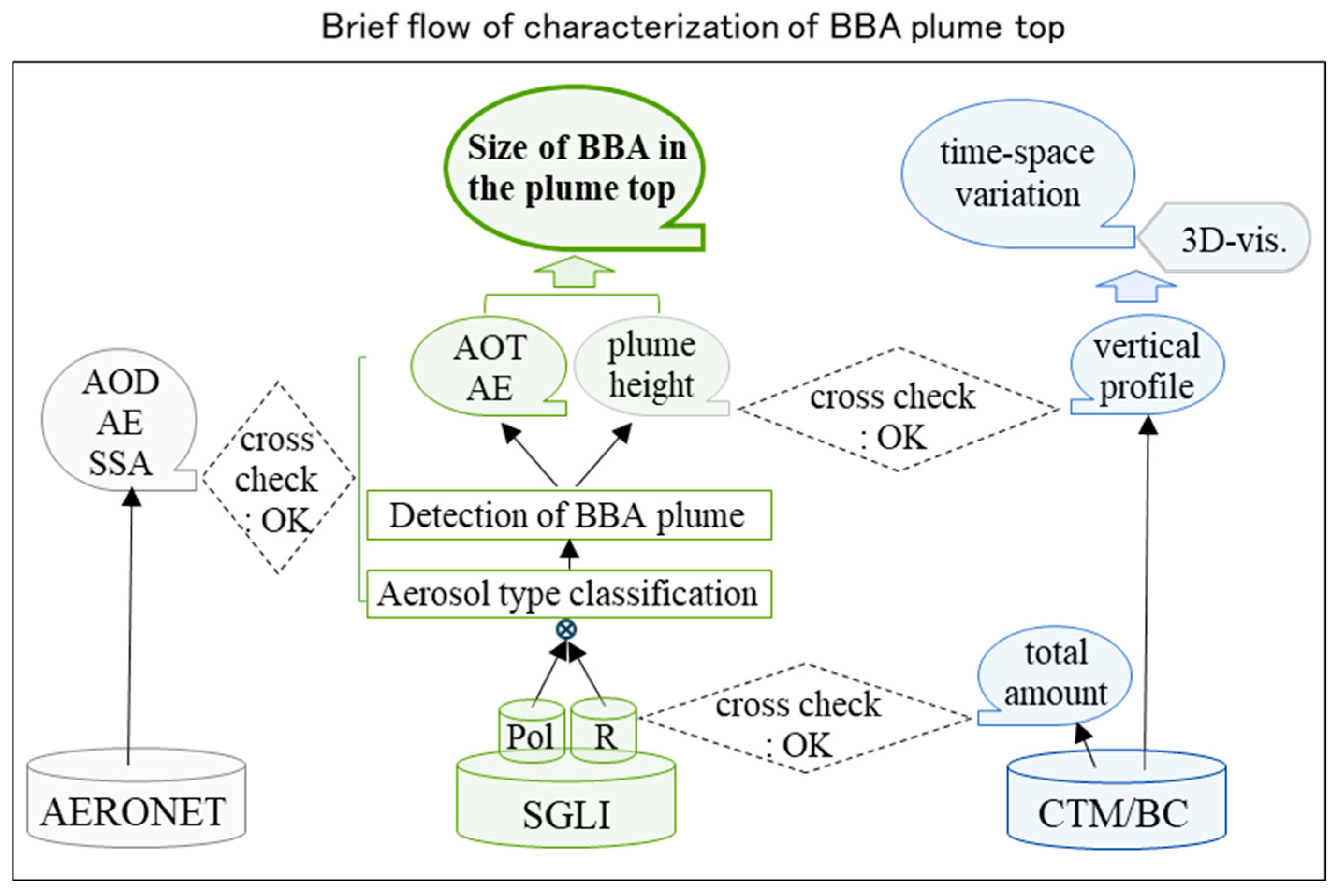
A flowchart of the study approach is shown in Figure 3. The SGLI reflectance (R) and total BC amount simulated by the CTM were successfully cross-correlated [40]. The classification of aerosol types and the detection of BBA plumes are performed using SGLI near-UV and polarization data. We compare the derived plume height with the aerosol vertical profile simulated by the CTM. SGLI-derived aerosol optical properties, such as AOT, are validated against ground-based AERONET observation data. AOD in AERONET data refers to aerosol optical depth, which is the same as AOT. Additionally, SSA in AERONET data represents single scattering albedo. Furthermore, this study investigates the relationship between plume top height and the derived aerosol optical properties, specifically AOT and AE. Using these results, we analyze the relationship between BBA particle size at the plume top and the plume height. The BBA distribution simulated by CTM is visualized in 3D for clarity. We also examine the temporal evolution of the distribution. Geostationary Operational Environmental Satellite (GOES) data were utilized to investigate temporal evolution. GOES comprises a series of weather satellites in the USA that have been in operation since 1975. GOES satellites are not limited to weather but also contribute to global environmental observations. Notably, Google uses GOES observations and hotspot data [40].

3. Result

3.1. California Forest Fires in September 2020

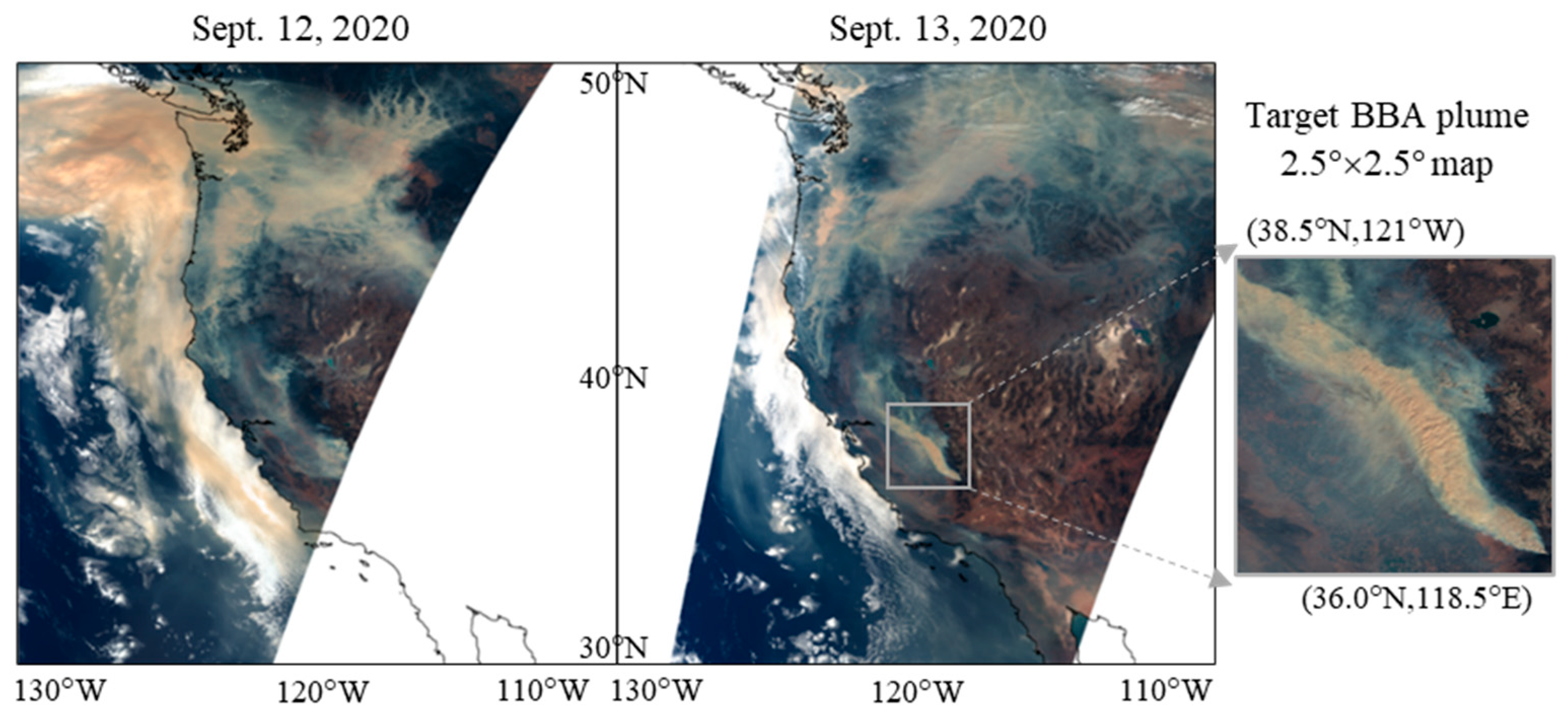
In recent years, large-scale forest fires have occurred almost annually in the northwestern coastal areas of North America from late summer to autumn. During this season, the combination of high temperatures and dry conditions enables the occurrence of large-scale fires, not necessarily under strong wind conditions, and even from small-scale triggers such as dry thunderstorms. Figure 4 presents color composite images (R, G, B) corresponding to (674, 530, 443 nm) with a 250 m spatial resolution for large-scale forest fires observed by the SGLI in California on 12–13 September 2020. The image from 12 September exhibits thick masses of smoke from wildfires in the upper area, seemingly drawn towards the ocean, covering the West Coast with a thick smoky haze. The image from 13 September shows the smoke air mass approaching land owing to the westerly winds and combining with fresh smoke from the wildfires. Evidently, even a single overpass of wide-swath sub-kilometer-scale satellite imagery reveals the advection of smoke generated by wildfires. The figure on the right shows an enlarged view of the BBA plume area targeted for analysis in this section. A highly distinctive smoke plume can be observed.
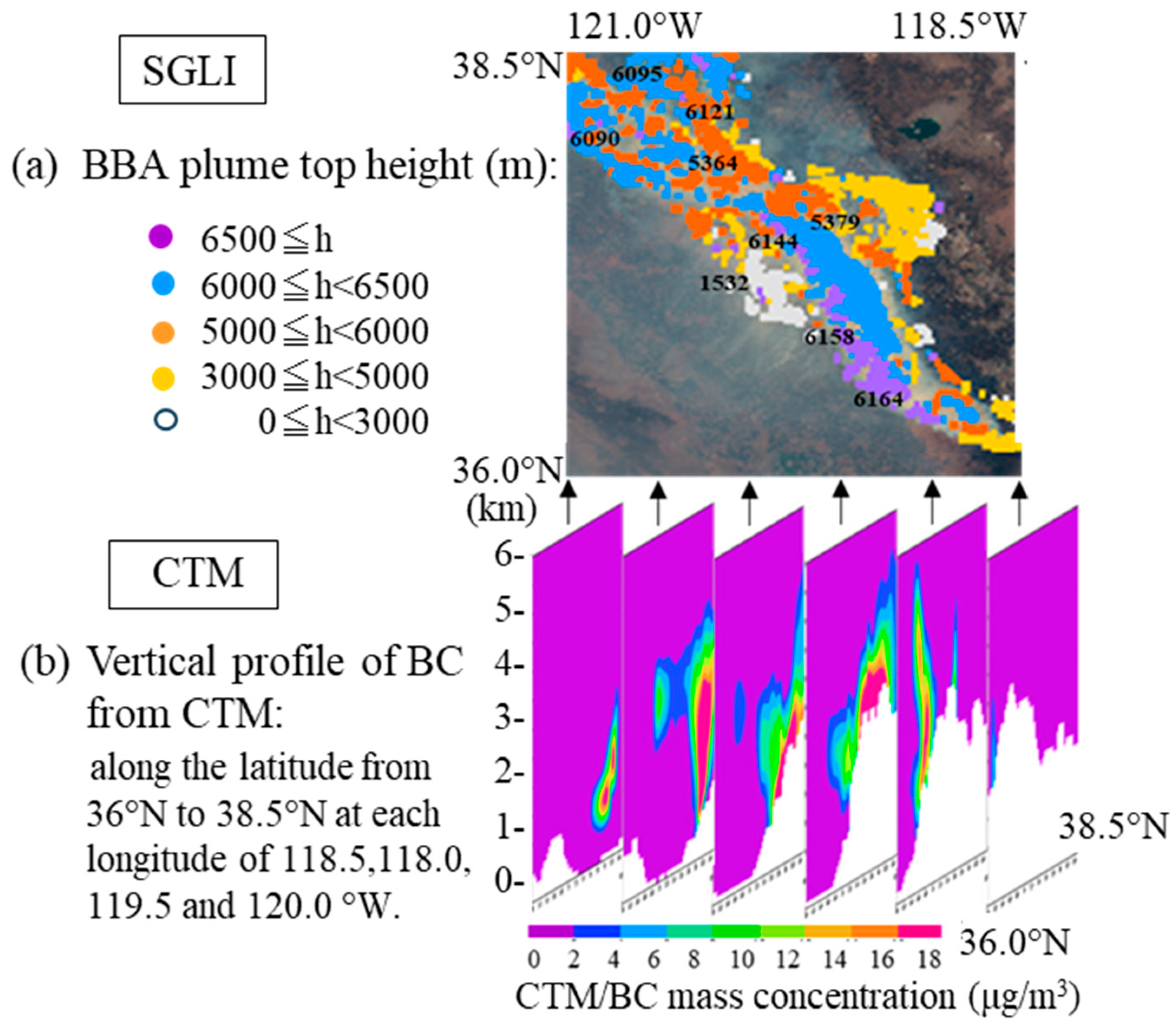
The focus of this 2020 Californian forest fire case is the distinctive BBA plume that is observed on 13 September, as shown in the rightmost image in Figure 4. Figure 5a shows the height of the BBA plume estimated from SGLI two-directional measurements. The plume heights are classified into several bins, taking into account the precision of the measurements as described in a previous study [19]. The blue and violet areas represent height ≥ 6 km, the orange areas between 5 and 6 km, and the yellow areas between 3 and 5 km. The height less than 3 km is shown in light gray. Figure 5b presents the corresponding CTM-simulated black carbon (BC) concentration (µm/m3) in North-to-South vertical cross sections. The cross sections cover from 36°N to 38.5°N latitudes at 6 discrete longitudes from 118.5°W to 121°W in 0.5° steps. The white color shading near the bottom of Figure 5b represents mountains that peak around 3 km, indicating that the plume sources are located in a mountainous area. The BC released from the fire activities stretches from the surface to 6 km altitude. Here, we compare the value calculated from SGLI two-directional data with the value simulated from CTM for the estimated BBA plume top height observed on 13 September 2020. The plume height simulated by the CTM did not show discrepancies with the stereoscopic estimation from the SGLI. The numerical CTM was partially validated by the BBA plume heights estimated from the SGLI data. Quantitative comparisons regarding CTM reproducibility have been conducted in prior studies, demonstrating a correlation coefficient of 0.68 between SGLI reflectance data (R) and the total black carbon (BC) amount simulated by CTM [39].
The 3D structure of the forest fires can be observed from the CTM. Subsequently, the accuracy of the numerical CTM simulations for this event was verified. Figure 5 shows that the CTM/BC simulation results were consistent with the products estimated from the SGLI data. The regional CTM was validated using SGLI satellite data, considering the BBA plume top height.

3.1.1. Characterization of BBA in the Plume Top

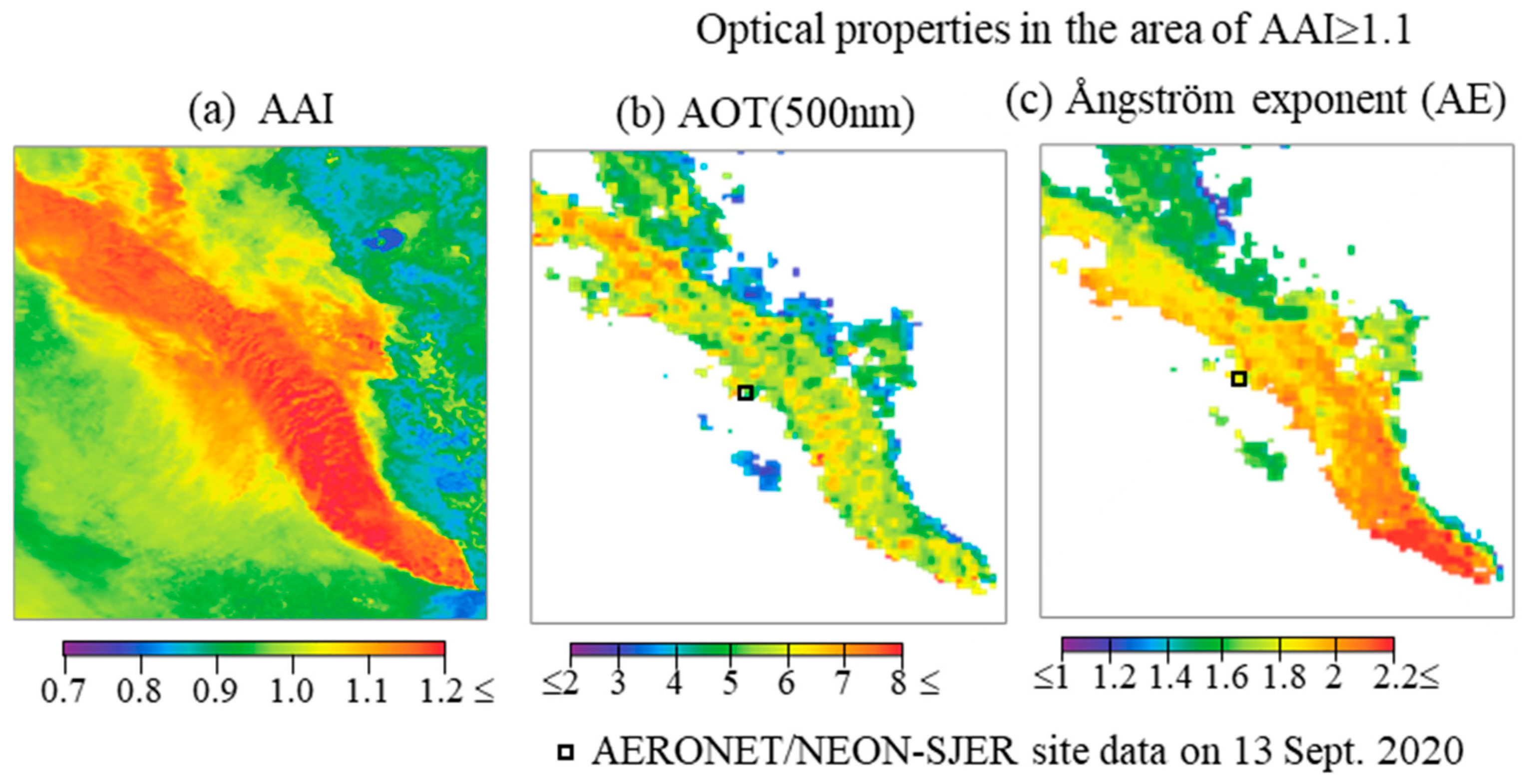
Figure 6a presents the AAI values over the same area as that in Figure 5a. The AAI values of the BBA plumes were ≥1.1, categorizing them as severe BBA. Figure 6b,c presents the retrieved AOT and AE from the SGLI measurements using the algorithm described in the previous study [3] over the area with AAI ≥ 1.1. The filtering by AAI limits the analysis to the area over the BBA plume, as shown in Figure 6. Although the details are described in reference [3], it should be highlighted that the retrieval algorithm fully benefits from the distinct features of SGLI: two near-UV wavelengths at 380 nm and 412 nm, and two polarization channels at 674 nm and 869 nm. The range of input parameters was expanded to retrieve more realistic BBA properties. Figure 6b demonstrates that retrieved AOT at 500 nm is greater than 4 over the BBA plume, indicating that the aerosol loading is significant, and reconfirming that AAI ≥ 1.1 is a good indicator to locate extremely dense BBA. Figure 6c shows that AE values exceed 1.6 over the thick plume, indicating that the BBA plume primarily consists of fine-mode particles. Naturally, intense wildfires blow finer soot particles to higher altitudes [41]. Consequently, these particles travel farther on upper-level air currents, spreading air pollution. This phenomenon is discussed in Section 3.1.3. As a result, BBA emitted from large wildfires poses a serious global threat. The explosive release of BBA from wildfires causes long-range transport, migration, and air pollution, leading to significant health impacts and further threats to society and the climate.
The small open square in Figure 6 shows the position of the NASA/AERONET/NEON-SJER site, where AOT and AE values are reported as 5.34 and 1.68, respectively, from AERONET measurements. The AERONET/NEON-SJER site data were averaged over ±30 min of overpassing the SGLI. The correlation coefficients between our analysis and the AERONET data were 0.88 and 0.92 for the AOT and AE values, respectively, in the case of an expanded target area including multiple AERONET sites other than NEON-SJER [3]. Specifically, since no AERONET data are perfectly synchronized with satellite observations, we use the average of AERONET data from the 30-min intervals before and after the satellite pass for comparison. The values measured at NEON-SJER are colored within the small black squares in Figure 6b,c. Our retrieval results from the space-based SGLI observations demonstrated consistency with NEON-SJER measurements.
The combination of satellite-based AOT, AE, and plume top height reveals the correlation between them, adding the dynamic aspect to the case study. Table 2 shows the average values of the AOT (500 nm) and AE within each class of BBA plume top height (in meters): h ≥ 6500, 6500 > h ≥ 6000, 6000 > h ≥ 5000, and 5000 > h ≥ 3000 from top to bottom. In all classes of plume top heights, the AE value significantly exceeded 1.2, indicating that the BBA is predominantly composed of small particles, presumably carbonaceous aerosols. The average AOT and AE values in each plume top height class present a positive correlation with the height. That is, the higher the top of the plume, the thicker the BBA plume optical thickness and the smaller the particle size. This aligns with the simple law that large particles fall faster than small particles in the atmosphere [42]. Small particles that compose the observed BBA plume have longer residence times than large particles [43], and they are more prevalent in the free troposphere as background aerosols [44].

3.1.2. The Presence of Small Particles Implied from Polarized Reflectance

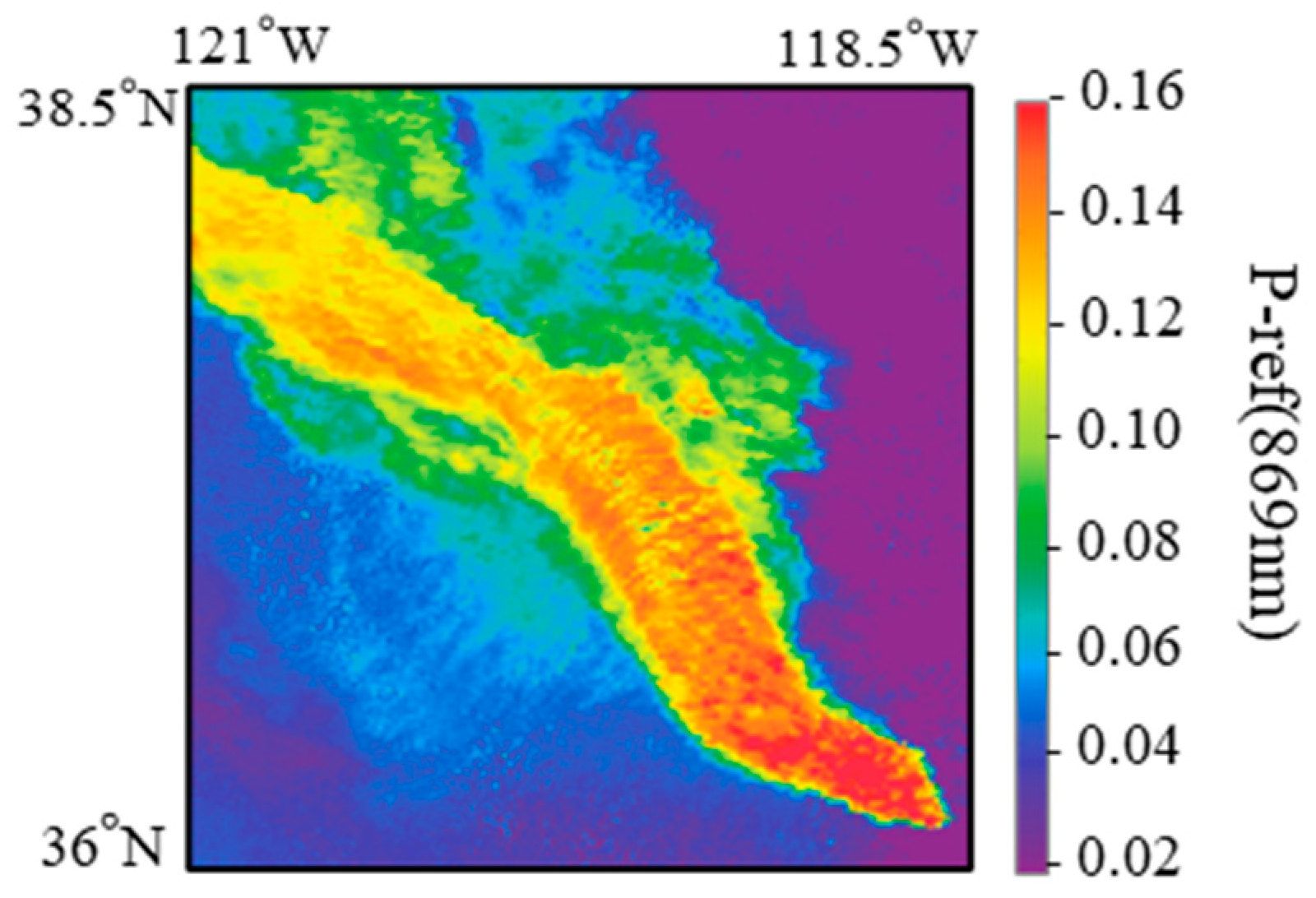
While the retrieved AE values are the best estimate based on the combination of multi-spectral and polarization measurements, SGLI-measured polarization itself also indicates the presence of small particles. Figure 7 shows the top-of-atmosphere polarized reflectance (P-ref) at a wavelength of 869 nm. To enable comparison with the top height of the BBA plume, the area in Figure 7 is the same as that in Figure 5a, and the SGLI observation data used is for the same region and time period. The individual pixels in Figure 5a and Figure 7 cannot be directly compared due to parallax; however, the BBA plume top height class and P-ref (869 nm) are positively correlated. That is, the higher the plume, the higher the P-ref.
Furthermore, radiative transfer simulations (see Appendix A for details) also revealed that polarization is sensitive to fine particles in the upper atmosphere, with smaller particle sizes yielding greater polarized reflectance (P-ref). In other words, our light scattering and radiative transfer simulations demonstrate in Figure A1 that P-ref increases as the fine-mode fraction (f) increases (i.e., particle size decreases).

3.1.3. Sequential Changes of BBA Plume with GOES

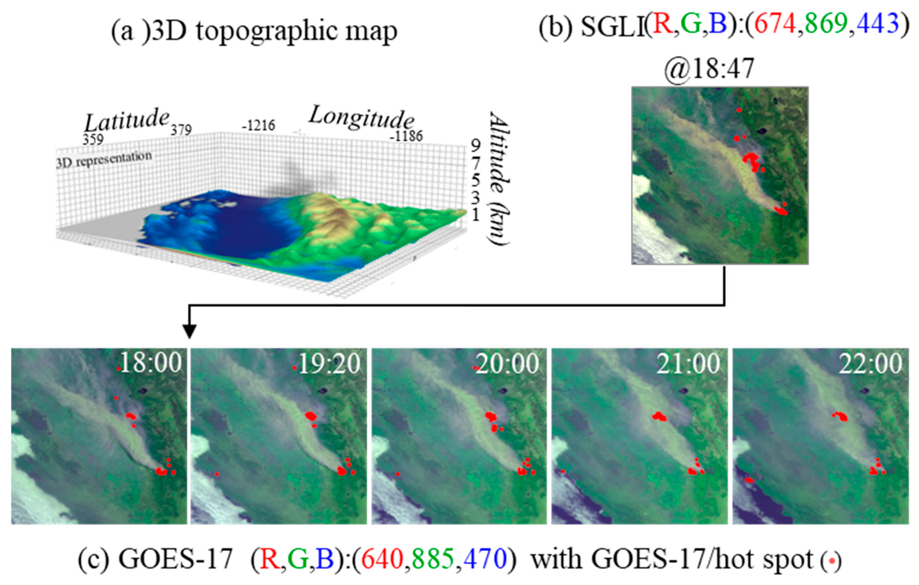
Figure 8a is the bird’s-eye view of the topography over the area of interest (35°N–39°N, 118°W–122°W) with the vertical axis representing the altitude (in kilometers). The central flatland in Figure 8a features a complex topography, with the Pacific Ocean blocked to the west by the Coastal Mountains and the high Sierra Nevada Mountains to the east. The fire started and spread on the west side of the Sierra Nevada Mountains, where hotspots were scattered, resulting in the generation of complex local winds and large amounts of BBA. Consequently, the characteristic BBA plume was formed.
The SGLI observation time was approximately 18:47 UTC on 13 September 2020 (Figure 8b). The GOES images (Figure 8c) are useful for understanding the temporal evolution of the BBA plume. GOES comprises a series of weather satellites in the USA that have been in operation since 1975. For comparison, the SGLI image observed at 18:47 is shown in Figure 8b. The color composites slightly differed from each other because of the slightly different spectral channels and the different spatial resolution (2 km for GOES and 250 m for SGLI), but the GOES and SGLI images demonstrate the consistent spatiotemporal variations. After passing the SGLI, heavy smoke flowed eastward, and at 22:00, the characteristic shape of the BBA plume captured by the SGLI collapsed. The time-series imagery of the BBA plumes with hotspots (denoted by orange dots) derived from GOES in Figure 8c.
Based on a comparison and combination of the time-sequential images by GOES, the smoke spread from the fire source hotspots into the atmosphere following the wind direction. Figure 8b,c shows the temporal variations of the BBA plume. Part of the BBA smoke plume is blocked by the mountains on the east side, and the BBA smoke plume flows in a northwesterly direction, continuing in this state until around the time of observation by the SGLI sensor. However, as the fire intensified and smoke rose over the mountains (see Figure 8c), the smoke plume gradually turned eastward, as if being dragged by the prevailing westerly winds aloft.

3.2. Sumatra Peatland Fires in September 2019

While the first case study over California is the emission from unintended forest fires, the second case study over Sumatra in Indonesia involves severe wildfires triggered by human activity. Slash-and-burn agriculture in this region causes peat fires, resulting in the release of large amounts of BBAs, typically peaking during the dry season from July to October. The emitted BBA travels as far as Malaysia, Singapore, southern Thailand, and the Philippines, causing widespread air pollution and resulting in health hazards such as breathing difficulties [9,45]. As a representative example of BBAs disaster, the Sumatra peatland fire in September 2019 was selected for analysis.

3.2.1. Retrieval of Optical Properties of BBA Plume

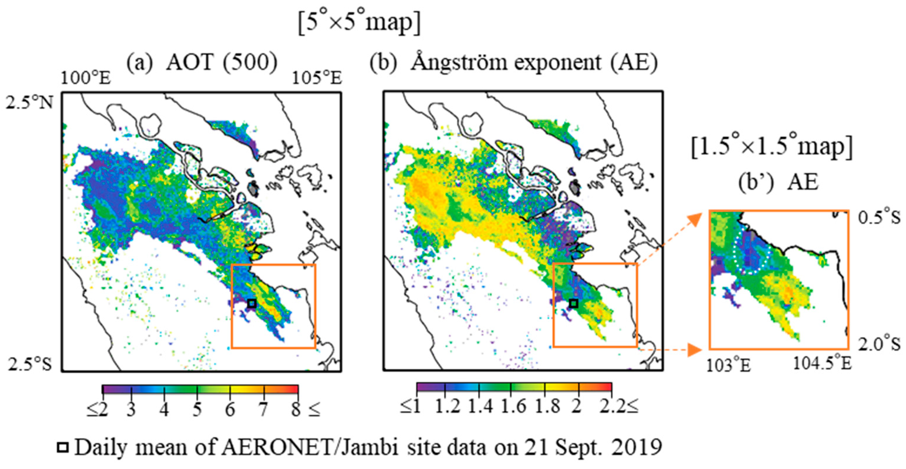
Figure 9 presents the AOT (500 nm) and AE retrieved from the SGLI measurements using the algorithm described in the previous study [3] over the area with AAI ≥ 1.1, together with the position of the NASA/AERONET/Jambi site with a square (1.63°S, 103.64°E). The color within the square indicates the daily mean AERONET measurements on 21 September 2019, which do not indicate a contradiction. The retrieved values should be compared with those at the time of the SGLI passage over the Jambi site, but owing to the lack of matching observation values, daily average values were used. Although observing sunlight from the ground during an optically thick atmosphere, such as a BBA plume, is difficult, our retrieval results from space-based SGLI observations demonstrated consistency with ground measurements in the Jambi site. The orange squares indicate the areas of severe BBA, including the fire sources shown in Figure 9a,b.
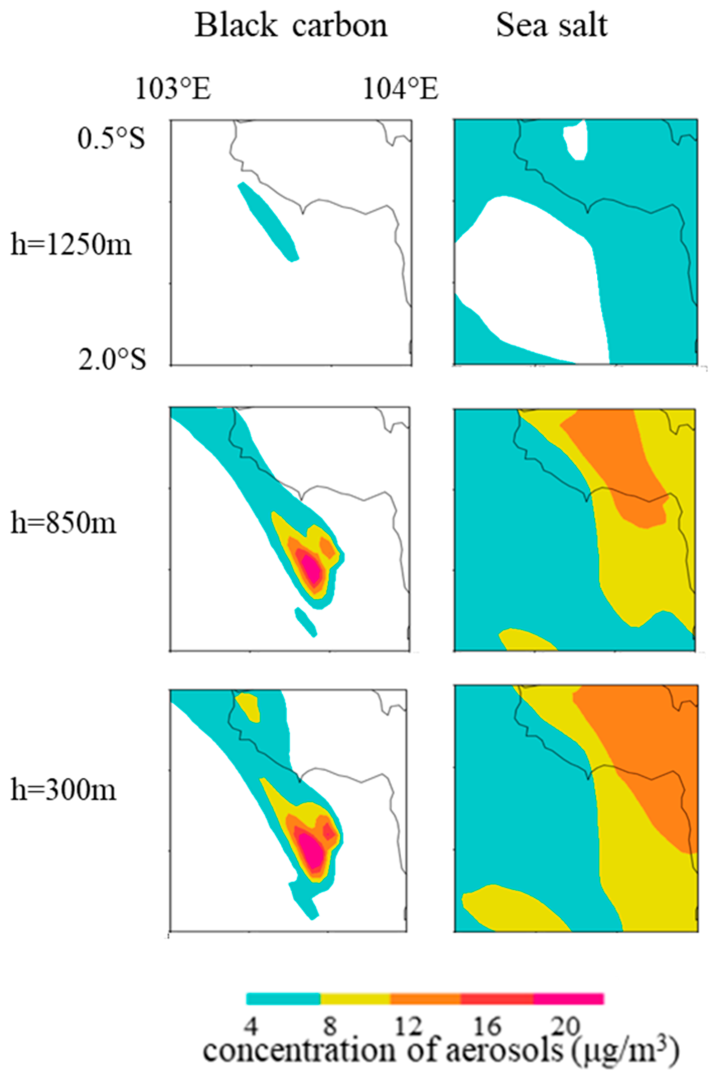
This wildfire occurred in the coastal lowlands along the eastern coast of Sumatra. As no highlands exist to block the easterly winds from the sea, the inflow of oceanic aerosols cannot be ignored. Figure 10 shows the CTM-simulated distribution of atmospheric particles in the same region and time as in Figure 9. The sea salt aerosol amounts were found to be as large as those of BC. Figure 10 shows areas with aerosol concentrations of ≥4 μg/m3 using color coding to highlight the regions with high aerosol amounts. While both BC and oceanic aerosol amounts decrease with increasing altitude, the horizontal distributions are different. Oceanic aerosols are primarily over the ocean but propagate toward the inland. The intrusion of oceanic aerosol may explain the low AE values in Figure 9 along the coast, particularly the area enclosed by the white dotted line in Figure 9b′.

3.2.2. Characterization of BBA Plume Top Height

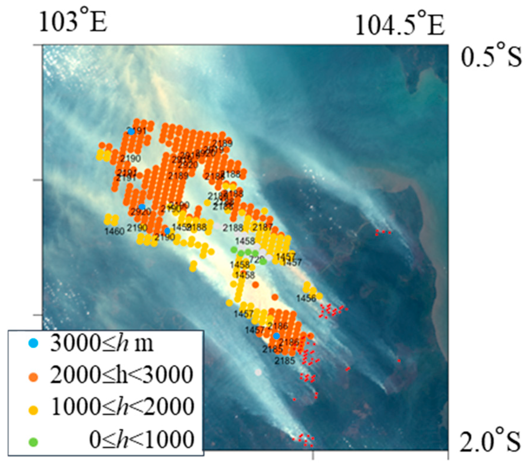
Figure 11 shows the height of the BBA plume estimated from SGLI two-directional measurements. The plume heights are classified into several bins; the light blue ellipses represent height ≥ 3 km, orange ellipses between 2 and 3 km, yellow ellipses 1 and 2 km, and green ellipses below 1 km. A large part of the successful estimates indicates that the plume top height was between 1 km and 3 km. A large number of hotspots, high temperatures as determined by Moderate Resolution Imaging Spectroradiometer (MODIS) satellite imagery, were observed in Sumatra Island in this period.
Similar to the analysis for the California wildfire, the relationship between the BBA plume top height classes and the optical properties of BBA smoke from forest fires in Sumatra is presented in Table 3. The average AOT and AE values in each plume top height class present a positive correlation to the height, similar to Table 2. That is, the higher the top of the plume, the greater the optical thickness of the BBA plume and the smaller the particle size.
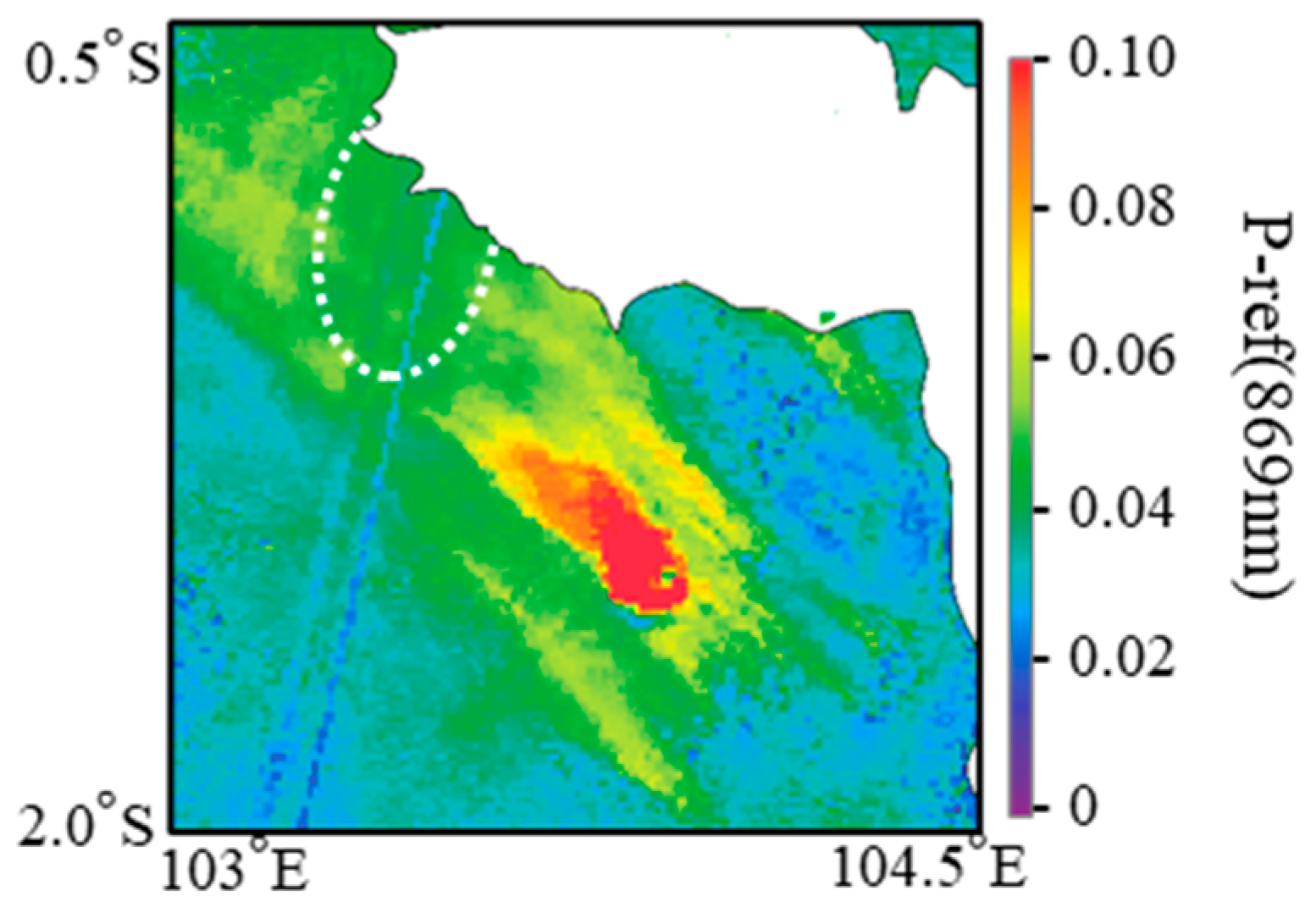
In order to reconfirm the results in Table 3, the polarized reflectance (P-ref (869)) observed by the SGLI was presented in Figure 12. For comparison with the top height of the BBA plume, the area and the SGLI observation data in Figure 11 are the same as those in Figure 12. Note that the two artificial noise lines colored green, light blue, and blue from near the top center to the bottom left of Figure 12 are caused by the mounting positions of the two polarizing filters on the line Charge Coupled Device (CCD) sensor. The individual pixels in Figure 11 and Figure 12 cannot be directly compared; however, the BBA plume top height class and P-ref (869 nm) are positively correlated in the area where the mixing of oceanic aerosols is negligible. Similar explanations have already been provided in Section 3.1.1 and Section 3.1.2 together with SGLI images, but here we revisit the polarized reflectance (P-ref) and plume top height. Since the normalized cross-correlation template matching method is used for plume height estimation, there is no pixel-by-pixel correspondence. Table 2 and Table 3 show the average values of AOT and AE for each plume height group, which are proportional to the plume height. From Figure A1, since AOT and P-ref clearly show a monotonic increasing trend, P-ref can be interpreted as having a positive correlation with plume height. Namely, the higher the plume, the higher the P-ref (869). The white dotted line in Figure 12, corresponding to the white dotted line in Figure 9b′, indicates regions where the mixing of oceanic aerosols cannot be ignored.

3.3. Summary of Two Case Studies

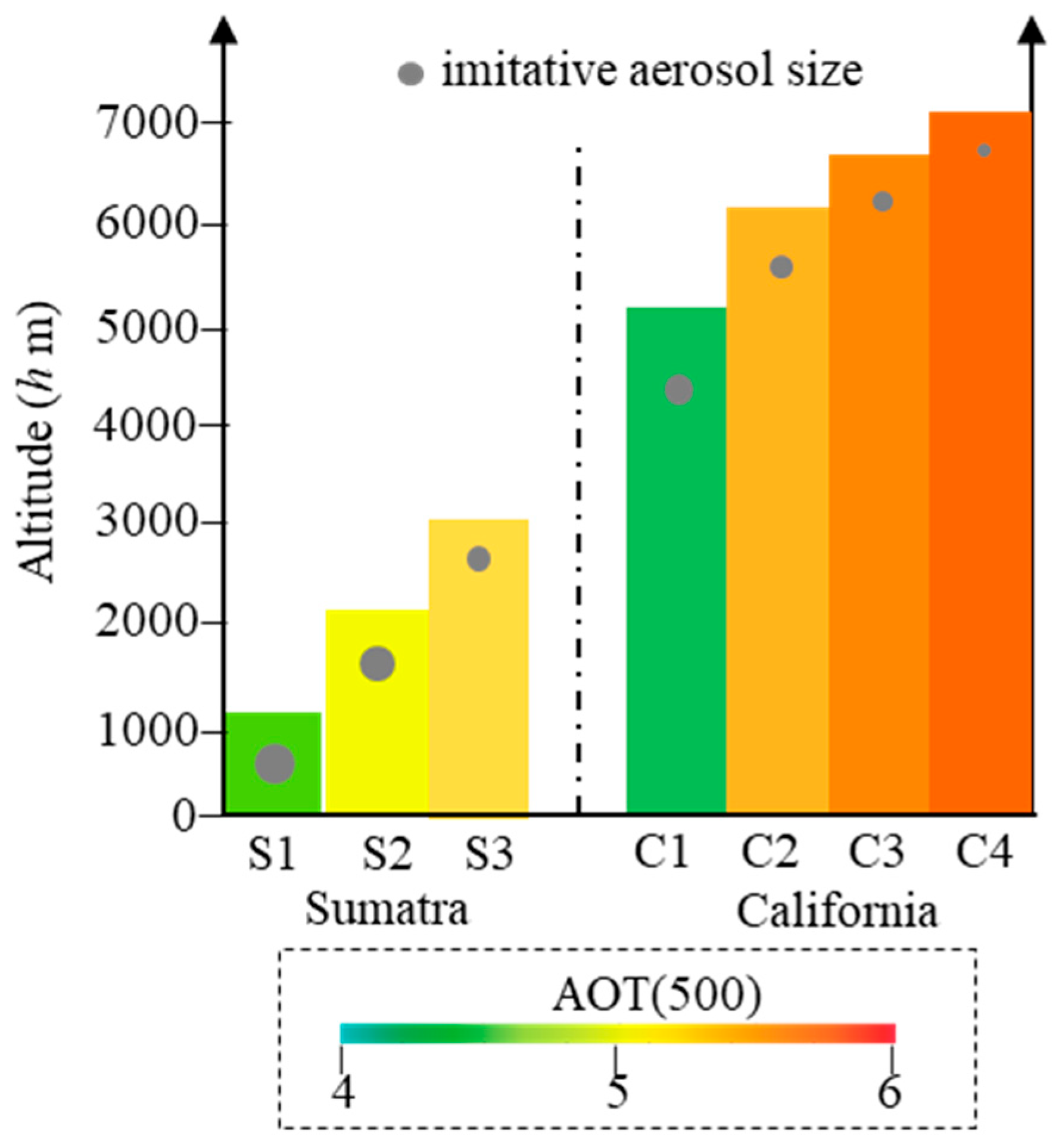
For the two case studies, optical properties such as AOT and AE were retrieved from multiple scattering calculations in the vector radiation field, and the retrieved values were validated by ground measurements of NASA/AERONET. The average AOT and AE values are positively correlated to the top height of the BBA plume in both California and Sumatra, as shown in Table 2 and Table 3, respectively. This indicates that the higher the BBA plume top, the thicker the AOT and the smaller the aerosol size (Figure 13). Each averaged value of AOT (500 nm) was colored according to the bottom color scale. The dark gray circles represent hypothetical changes in the BBA particle size and are not the actual size. This finding aligns with the simple law that large particles fall faster than small particles in the atmosphere. Because small particles have longer residence times than large particles, they are more prevalent in the upper atmosphere. In reality, the composition, shape, and size of BBA particles are likely to vary considerably depending on the source of the wildfire and the surrounding environment. Nevertheless, the average values observed from satellites at an altitude of approximately 700 km exhibit major characteristics that remain after suppressing individual variations.

4. Discussion

This study elucidated the 3D characteristics of BBA plumes during large-scale wildfires. The scale of fires and their influence on advection, which is an important factor in environmental and climate change, were investigated using typical BBA events. As shown in the previous section, interestingly, the higher the BBA plume top, the thicker the AOT, and the smaller the aerosol particle size. This results in a higher proportion of fine particles in the upper atmosphere. Furthermore, the stereoscopic plume top height was positively correlated to the measured polarized reflectance, which is negatively correlated to the particle size according to the RT simulations. It should be noted that the findings derived from applying various processes to satellite data are based on two case studies. However, these results are consistent with the fundamental physical principle that larger atmospheric particles exhibit higher settling velocities than smaller particles within the troposphere. Although the composition, shape, and size of BBA particles are likely to vary depending on the wildfire, the primary characteristics were succinctly captured from an altitude of 800 km, despite containing individual complex changes.

5. Conclusions

This study characterized the three-dimensional properties of BBA plumes from large-scale wildfires in North America and Indonesia by integrating SGLI satellite observations and CTM simulations. Through the synergistic use of near-ultraviolet and polarization data, we successfully derived the spatial and vertical distributions of BBA, including plume top height and optical properties. The most significant finding of this research is the positive correlation between the BBA plume top height and its optical characteristics (AOT and AE). Our analysis demonstrates that higher plume tops are associated with increased optical thickness and smaller particle sizes. This discovery is crucial, as it suggests that the vertical injection height of a wildfire plume is intrinsically linked to its microphysical evolution and concentration. By clarifying the detailed particle characteristics at the plume top, this research contributes to more accurate predictions of BBA advection, atmospheric lifetime, and their subsequent environmental impacts.
The algorithms and results proposed in this study could also be applied to the next subject to monitor the aerosol hazards, such as dust events, volcanic eruptions, dense PM pollution, and so on.

Author Contributions

Conceptualization, M.N. and S.M.; methodology, M.N.; software, S.H.; validation, M.N., S.M. and S.H.; formal analysis, M.N.; investigation, S.M.; resources, M.N.; data curation, S.H.; writing—original draft preparation, M.N.; writing—review and editing, M.N. and S.M.; visualization, M.N., S.M. and S.H.; supervision, S.M.; project administration, S.M.; funding acquisition, S.M. All authors have read and agreed to the published version of the manuscript.

Funding

This research was funded by the Global Change Observation Mission-Climate Project of JAXA (JX-ER4GCF).

Data Availability Statement

The original contributions presented in the study are included in the article; further inquiries can be directed to the corresponding author.

Acknowledgments

The authors express their gratitude to Itaru Sano and Toshiyuki Fujito for assisting in calculating radiative transfer calculations and the satellite data preparation, respectively; JAXA for distributing the observed data using GCOM-C/SGLI; and NASA for providing the AERONET and GOES data.

Conflicts of Interest

The authors declare no conflicts of interest.

Abbreviations

The following abbreviations are used in this manuscript:
AAIAbsorption aerosol index
AEÅngström Exponent
AERONETAErosol RObotic NETwork
AOTAerosol Optical Thickness
AODAerosol Optical Depth
BBABiomass burning aerosols
BCBlack carbon
CCDCharge Coupled Device
CTMChemical transport model
GCOM-CGlobal Change Observation Mission-C
GOESGeostationary Operational Environmental Satellite
IRInfrared
MISRMulti-angle Imaging SpectroRadiometer
PRIPolarized radiance index
RTRadiative transfer
SCALEScalable Computing for Advanced Library and the Environment Regional Model
SGLISecond-generation Global Imager
SSASingle Scattering Albedo
UVUltraviolet

Appendix A. Vector Radiative Transfer Calculation of Reflectance from the Top of the Atmosphere
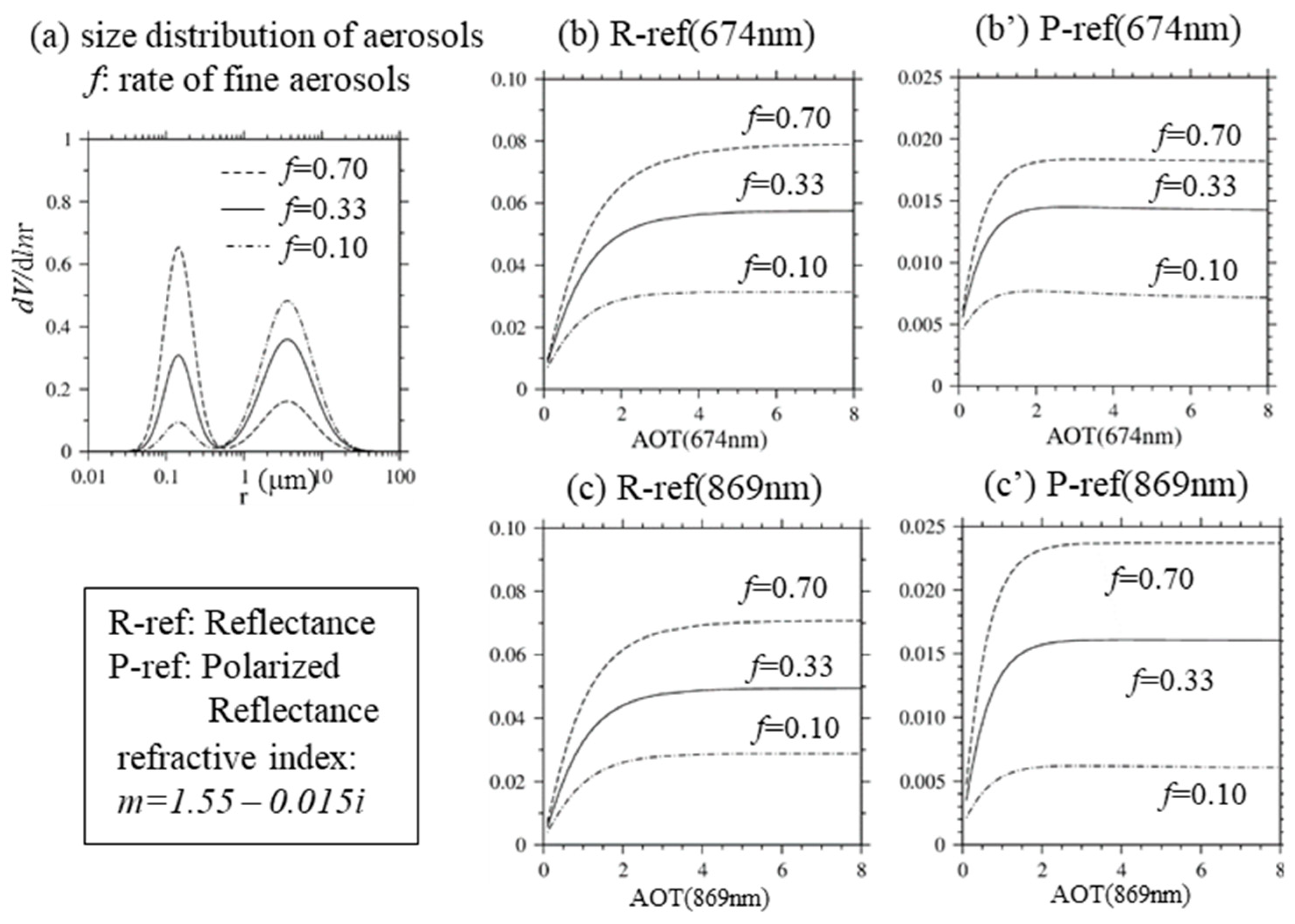
In this study, a vector-type RT simulation method was adopted to utilize SGLI polarization band (PL1 and PL2) data. The algorithms used were based on the vector method of adding-doubling [46,47]. The space-borne sensors measured the upwelling radiance at the top of the atmosphere, which is called reflectance from the AOT (λ) at a wavelength λ. The incident solar radiation in the direction of Ω 0 frequently interacts with such atmospheric particles as aerosols or molecules. Reflectance is defined to be the intensity vector of AOT in the direction of Ω . The direction of Ω is represented by the zenith angle ( θ ) and azimuth angle ( φ ). In radiative transfer calculation, the direction is typically defined by Ω = μ , φ , where μ is the cosine of the zenith angle θ (i.e., μ = cos θ ). Suppose an incident radiation of flux F in direction Ω 0 μ 0 , φ 0 is falling on the top of the atmosphere, taking R τ , Ω , Ω 0 as a matrix of reflectance from the AOT. The vector field of the adding-doubling method is described by Stokes parameters I , Q , U , V . Therefore, the reflectance matrix R and single-scattering phase matrix P ~ take the form of a 4 × 4 matrix. R-rad (λ) and P-rad (λ) are defined as the I- and polarized components of the reflectance matrix R at a wavelength λ, respectively. The polarized component P-ref (λ) is defined by Equation (2).
The basic property of RT simulations is the spectral AOT (λ). To elucidate this, we first determined the size and composition of the aerosol model. The aerosol size distribution is represented by bimodal (fine and coarse) log-normal distributions of particle volume, which are usually used according to accumulated NASA/AERONET data [48]. The aerosol size distribution can be expressed by a simple approximation with the unique variable of the fine particle fraction (f) of the volume concentration [34]. The aerosol composition was interpreted using a complex refractive index (m (λ) = n (λ)–k (λ)i). For BBAs, the real part (n) can be approximated by 1.55, and the imaginary part (k) is assumed to take values in the range of [0.005, 0.02] around the SGLI polarization band [49]. Figure A1 shows the numerical results for an RT simulation example for the carbonaceous aerosol model at λ = 674 and 869 nm, where a bimodal log-normal size distribution with a fine particle fraction (f) is adopted. As an example of the refractive index of a carbonaceous aerosol, m = 1.55–0.015i is assumed. The angle variables are represented by (θ, θ0, φ-φ0) based on the SGLI sun-satellite direction. For the example in Figure A1, the directional values are represented by (θ, θ0, φ-φ0) = (56.1°, 38.9°, 66.6°), which roughly corresponds to the NASA/AERONET site NEON_SJER on 13 September 2020.
Figure A1. R-ref and P-ref versus AOT for the carbonaceous aerosol model under refractive index m = 1.550–0.015i at the wavelengths of λ = 674 and 869 nm, where directional data approximately coincide with SGLI on 13 September 2020 over the NASA/AERONET/NEON_SJER site (37°N, 120°W) as an example. (a) Bimodal log-normal size distribution with fine particle fraction f, (b) R-ref and (b′) P-ref versus AOT at λ = 674 nm, (c) R-ref and (c′) P-ref versus AOT at λ = 869 nm.
Remotesensing 18 00747 g0a1
The variation of the R-ref and P-ref functions with AOT (Figure A1) indicates that while the function values and gradients vary with aerosol size and wavelength, the following trends are evident:
  • R-ref and P-ref are proportional to f,
  • R-ref and P-ref increase with AOT but converge at a certain AOT.
  • The converging AOT point is lower for a smaller f,
  • After convergence (i.e., reaching the maximum point), R-ref is invariable. Although the value and slope change with the variable, the approximate shape of the R-ref function remains unchanged.
  • After reaching its maximum value, P-ref shows a slight decrease along with the AOT owing to the reduction in polarizability caused by multiple light scattering.
  • The numerical results for both wavelengths are compared as follows:
    • For R-ref, no noticeable effect was observed on the absolute value, change in AOT, or change in f.
    • P-ref changes differently at the two wavelengths. P-ref (869 nm) exhibits a larger variation with respect to AOT and f than P-ref (674 nm).
Considering items 4 and 5, in optically thick atmospheres such as the BBA plume, the values of the P-ref and R-ref functions reflect the upper and entire atmosphere, respectively. In other words, polarization is sensitive to small particles in the upper atmosphere because the smaller the particle size, the larger the P-ref, particularly at a wavelength of 869 nm.

References

  1. Chow, F.; Yu, K.; Young, A.; James, E.; Grell, G.; Csiszar, I.; Tsidulko, M.; Freitas, S.; Pereira, G.; Giglio, L.; et al. High-Resolution Smoke Forecasting for the 2018 Camp Fire in California. Bull. Am. Meteorol. Soc. 2022, 103, E1531–E1552. [Google Scholar] [CrossRef]
  2. Makar, P.; Akingunola, A.; Chen, J.; Pabla, B.; Gong, W.; Stroud, C.; Sioris, C.; Anderson, K.; Cheung, P.; Zhang, J.; et al. Forest fire aerosol-weather feedback over western North America using a high-resolution, fully coupled, air quality model. Atmos. Chem. Phys. 2021, 21, 10557–10587. [Google Scholar] [CrossRef]
  3. Nakata, M.; Sano, I.; Mukai, S.; Kokhanovsky, A. Characterization of wildfire smoke over complex terrain using satellite observations, ground-based observations, and meteorological models. Remote Sens. 2022, 14, 2344. [Google Scholar] [CrossRef]
  4. Liu, J.C.; Pereira, G.; Uhl, S.A.; Bravo, M.A.; Bell, M.L. A systematic review of the physical health impacts from non-occupational exposure to wildfire smoke. Environ. Res. 2025, 136, 120–132. [Google Scholar] [CrossRef]
  5. Reid, C.E.; Brauer, M.; Johnston, F.H.; Jerrett, M.; Balmes, J.R.; Elliott, C.T. Critical review of health impacts of wildfire smoke exposure. Environ. Health Perspect. 2016, 124, 1334–1343. [Google Scholar] [CrossRef]
  6. Cascio, W.E. Wildland fire smoke and human health. Sci. Total Environ. 2018, 624, 586–595. [Google Scholar] [CrossRef]
  7. Dickman, K. The hidden toll of wildfire. Sci. Am. 2020, 322, 38–45. [Google Scholar] [CrossRef]
  8. IPCC. Climate Change 2021, The Physical Science Basis. Contribution of Working Group I to the Sixth Assessment Report of the Intergovernmental Panel on Climate Change; Cambridge University Press: Cambridge, UK, 2021. [Google Scholar]
  9. Hein, L.; Spadaro, J.V.; Oatro, B.; Hammer, M.; Sumarga, E.; Salmayenti, R.; Boer, R.; Tata, H.; Atmoko, D.; Castañeda, J. The health impacts of Indonesia peatland fires. Environ. Health 2022, 21, 62. [Google Scholar] [CrossRef]
  10. de Laat, A.; Vazquez-Navarro, M.; Theys, N.; Stammes, P. Analysis of properties of the 19 February 2018 volcanic eruption of mount Sinabung in S5P/TROPOMI and Himawari-8 satellite data. Nat. Hazards Earth Syst. Sci. 2020, 20, 1203–1217. [Google Scholar] [CrossRef]
  11. Taylor, I.A.; Grainger, R.G.; Prata, A.T.; Proud, S.R.; Mather, T.A.; Pyle, D.M. A satellite chronology of plumes from the April 2021 eruption of la Soufrière. St Vincent. Atmos. Chem. Phys. 2023, 23, 15209–15234. [Google Scholar] [CrossRef]
  12. Kilian, M.; Grewe1, V.; Jöckel1, P.; Kerkweg, A.; Mertens1, M.; Zahn, A.; Ziereis1, H. Ozone source attribution in polluted European areas during summer 2017 as simulated with MECO (n). Atmos. Chem. Phys 2024, 24, 13503–13523. [Google Scholar] [CrossRef]
  13. Muller, J.P.; Mandanayake, A.; Moroney, C.; Davies, R.; Diner, D.J.; Paradise, S. MISR stereoscopic image matchers: Techniques and results. IEEE Trans. Geosci. Remote Sens. 2002, 40, 1547–1559. [Google Scholar] [CrossRef]
  14. Kahn, R.A.; Li, W.-H.; Moroney, C.; Diner, D.J.; Martonchik, J.V.; Fishbein, E. Aerosol source plume physical characteristics from space-based multi-angle imaging. J. Geophys. Res. 2007, 112, D11205. [Google Scholar]
  15. Kahn, R.A.; Chen, Y.; Nelson, D.L.; Leung, F.-Y.; Li, Q.; Diner, D.J.; Logan, J.A. Wildfire smoke injection heights: Two perspectives from space. Geophys. Res. Lett. 2008, 35, L04809. [Google Scholar] [CrossRef]
  16. Limbacher, E.; Kahn, A.; Lee, J. The new MISR research aerosol retrieval algorithm: A multi-angle, multi-spectral, bounded-variable least squares retrieval of aerosols particle properties over both land and water. Atmos. Meas. Tech. 2022, 15, 6865–6887. [Google Scholar] [CrossRef]
  17. Diner, D.J.; Beckert, J.C.; Reilly, T.H.; Bruegge, C.J.; Conel, J.E.; Kahn, R.A.; Martonchik, J.V.; Ackerman, T.P.; Davies, R.; Gerstl, S.A.; et al. Multi-angle Imaging SpectroRadiometer (MISR)—Instrument description and experiment overview. IEEE Trans. Geosci. Remote Sens. 1998, 36, 1072–1087. [Google Scholar] [CrossRef]
  18. Diner, J.; Beckert, C.; Bothwell, W.; Rodriguez, I. Performance of the MISR instrument during its first 20 months in earth orbit. IEEE Trans. Geosci. Remote Sens. 2002, 40, 1449–1466. [Google Scholar] [CrossRef]
  19. Hioki, S.; Funatomi, T.; Nakata, M.; Mukai, S.; Kidode, M. Stereoscopic height estimation of biomass burning aerosol and volcanic ash plumes by the second-generation global imager (SGLI). Remote Sens. 2024, 13193, 72–79. [Google Scholar]
  20. Kajino, M.; Deushi, M.; Sekiyama, T.T.; Oshima, N.; Yumimoto, K.; Tanaka, T.Y.; Ching, J.; Hashimoto, A.; Yamamoto, T.; Ikegami, M.; et al. Comparison of three aerosol representations of NHM-Chem (v1.0) for the simulations of air quality and climate-relevant variables. Geosci. Model Dev. 2021, 14, 2235–2264. [Google Scholar] [CrossRef]
  21. Nakata, M.; Kajino, M.; Sato, Y. Effects of mountains on aerosols determined by AERONET/DRAGON/J-ALPS measurements and regional model simulations. Earth Space Sci. 2021, 8, e2021EA001972. [Google Scholar] [CrossRef]
  22. Nishizawa, S.; Yashiro, H.; Sato, Y.; Miyamoto, Y.; Tomita, H. Influence of grid aspect ratio on planetary boundary layer turbulence in large-eddy simulations. Geosci. Model Dev. 2015, 8, 3393–3491. [Google Scholar] [CrossRef]
  23. Sato, Y.; Nishizawa, S.; Yashiro, H.; Miyamoto, Y.; Kajikawa, Y.; Tomita, H. Impacts of cloud microphysics on trade wind cumulus: Which cloud microphysics processes contribute to the diversity in a large eddy simulation. Prog. Earth Planet. Sci. 2015, 2, 23. [Google Scholar] [CrossRef]
  24. Giovannini, L.; Laiti, L.; Serafin, S.; Zardi, D. The thermally driven diurnal wind system of the Adige Valley in the Italian Alps. Q. J. R. Meteorol. Soc. 2017, 143, 2389–2402. [Google Scholar] [CrossRef]
  25. Schmidli, J.; Böing, S.; Fuhrer, O. Accuracy of simulated diurnal valley winds in the Swiss Alps: Influence of grid resolution. Atmosphere 2018, 9, 196. [Google Scholar] [CrossRef]
  26. Zhang, Z.; Xu, X.; Qiao, L.; Gong, D.; Kim, S.; Wang, Y.; Mao, R. Numerical simulations of the effects of regional topography on haze pollution in Beijing. Sci. Rep. 2018, 8, 5504. [Google Scholar] [CrossRef]
  27. Eck, T.; Holben, B.; Reid, J.; Giles, D.; Rivas, M.; Singh, R.; Tripathi, S.; Bruegge, C.; Platnick, S.; Arnold, G.; et al. Fog- and cloud-induced aerosol modification observed by the Aerosol Robotic Network (AERONET). J. Geophys. Res. 2012, 117, D07206. [Google Scholar] [CrossRef]
  28. Mukai, S.; Nakata, M.; Sano, I.; Fujito, T. Derivation of BBA Plume Properties by Taking Advantage of the Characteristics of GCOM-C/SGLI. IEEE J. Sel. Top. Appl. Earth Obs. Remote Sens. 2024, 17, 9790–9796. [Google Scholar] [CrossRef]
  29. Zhu, L.; Martin, M.V.; Gatti, L.V.; Kahn, R.; Hecobian, A.; Fischer, E.V. Development and implementation of a new biomass burning emissions injection height scheme (BBEIH v1.0) for the GEOS-Chem model (v9-01-01). Geosci. Model Dev. 2018, 11, 4103–4116. [Google Scholar] [CrossRef]
  30. Nakata, M.; Mukai, S. Consideration of aerosol injection processes originating from wildfires in a chemical transport model. Remote Sens. 2024, 13193, 141–144. [Google Scholar]
  31. Mukai, S.; Hioki, S.; Nakata, M. Biomass burning plume from simultaneous observations of polarization and radiance at different viewing directions. Remote Sens. 2023, 15, 5405. [Google Scholar] [CrossRef]
  32. Imaoka, K.; Kachi, M.; Fujii, H.; Murakami, H.; Hori, M.; Ono, A.; Igarashi, T.; Nakagawa, K.; Oki, T.; Honda, Y.; et al. Global change observation mission (GCOM) for monitoring carbon, water cycles, and climate change. Proc. IEEE 2010, 98, 717–734. [Google Scholar] [CrossRef]
  33. Tores, O.; Bhartia, P.K.; Herman, J.R.; Ahmad, Z.; Gleason, J. Derivation of aerosol properties from satellite measurements of backscattered ultraviolet radiation: Theoretical basis. J. Geophys. Res. 1998, 103, 17099–17110. [Google Scholar] [CrossRef]
  34. Mukai, S.; Sano, I.; Nakata, M. Algorithms for the classification and characterization of aerosols: Utility verification of near-UV satellite observations. J. Appl. Remote Sens. 2019, 13, 01452. [Google Scholar] [CrossRef]
  35. Han, Z.; Ueda, H.; Matsuda, K.; Zhang, R.; Arao, K.; Kanai, Y.; Hasome, H. Model study on particle size segregation and deposition during Asian dust events in March 2002. J. Geophys. Res. 2004, 109, D19205. [Google Scholar] [CrossRef]
  36. Clarke, A.D.; Owens, S.R.; Zhou, J. An ultrafine sea-salt flux from breaking waves: Implications for cloud condensation nuclei in the remote marine atmosphere. J. Geophys. Res. 2006, 111, D06202. [Google Scholar] [CrossRef]
  37. Kajino, M.; Deushi, M.; Sekiyama, T.T.; Oshima, N.; Yumimoto, K.; Tanaka, T.T.; Ching, J.; Hashimoto, A.; Yamamoto, T.; Ikegami, M.; et al. NHM-Chem, the Japan Meteorological Agency’s regional meteorology—Chemistry model: Model evaluations toward the consis tent predictions of the chemical, physical, and optical properties of aerosols. J. Meteor. Soc. Jpn. 2019, 97, 337–374. [Google Scholar] [CrossRef]
  38. Kaiser, W.; Heil, A.; Andreae, O.; Benedetti, A.; Chubarova, N.; Jones, L.; Morcrette, J.; Razinger, M.; Schultz, G.; Suttie, M.; et al. Biomass burning emissions estimated with a global fire assimilation system based on observed fire radiative power. Biogeosciences 2012, 9, 527–554. [Google Scholar] [CrossRef]
  39. Nakata, M.; Mukai, S. Aerosol distribution due to wildfire in Sumatra, Indonesia considered from model simulation. Remote Sens. 2025, 17, 1657. [Google Scholar] [CrossRef]
  40. Colarco, P.; da Silva, A.; Chin, M.; Diehl, T. Online simulations of global aerosol distributions in the NASA GEOS-4 model and comparisons to satellite and ground-based aerosol optical depth. J. Geophys. Res. 2010, 115, D14207. [Google Scholar] [CrossRef]
  41. Bourgeois, Q.; Ekman, A.M.L.; Krejci, R. Aerosol transport over the Andes from the Amazon Basin to the remote Pacific Ocean: A multiyear CALIOP assessment. J. Geophys. Res. 2015, 120, 8411–8425. [Google Scholar] [CrossRef]
  42. Dietrich, W.E. Setting velocity of natural particles. Water Resour. Res. 1982, 18, 1615–1626. [Google Scholar] [CrossRef]
  43. Clarke, A.D.; Collins, W.G.; Rasche, P.J.; Kapustin, V.N.; Moore, K.; Howell, S.; Fuelberg, H.E. Dust and pollution transport on global scales: Aerosol measurements and model predictions. J. Geophys. Res. 2001, 106, 32555–32569. [Google Scholar] [CrossRef]
  44. Murphy, D.M.; Cziczo, D.J.; Froyd, K.D.; Hudson, P.K.; Matthew, B.M.; Middlebrook, A.M.; Peltier, R.E.; Sullivan, A.; Thomson, D.S.; Weber, R.J. Single-particle mass spectrometry of tropospheric aerosol particles. J. Geophys. Res. 2006, 111, D23S32. [Google Scholar] [CrossRef]
  45. Wulandari, E.; Mardianto, D.; Susilastuti, D.H.; Maryudi, A. Scholarly interest in forest fires in Indonesia: A bibliographical review. For. Soc 2022, 6, 609–619. [Google Scholar] [CrossRef]
  46. van de Hulst, H.C. A New Look at Multiple Scattering; NASA Institute for Space Studies: New York, NY, USA, 1963; 162p. [Google Scholar]
  47. Mukai, S.; Sano, I.; Takashima, T. Investigation of atmospheric aerosols based on polarization measurements and scattering simulations. Opt. Rev. 1996, 3, 487–491. [Google Scholar] [CrossRef]
  48. Omar, A.; Won, J.; Winker, D.; Yoon, S.; Dubovik, O.; McCormick, P. Development of global aerosol models using cluster analysis of aerosol robotic network (AERONET) measurements. J. Geophys. Res. 2005, 110, D10S14. [Google Scholar] [CrossRef]
  49. Oleg, D.; Sayer, A.; Hsu, N.; Eck, T.; Smirnov, A.; Holben, B. AERONET-based models of smoke-dominated aerosol near source regions and transported over ocean, and implications for satellite retrievals of aerosol optical depth. Atmos. Chem. Phys. 2014, 14, 11493–11523. [Google Scholar]
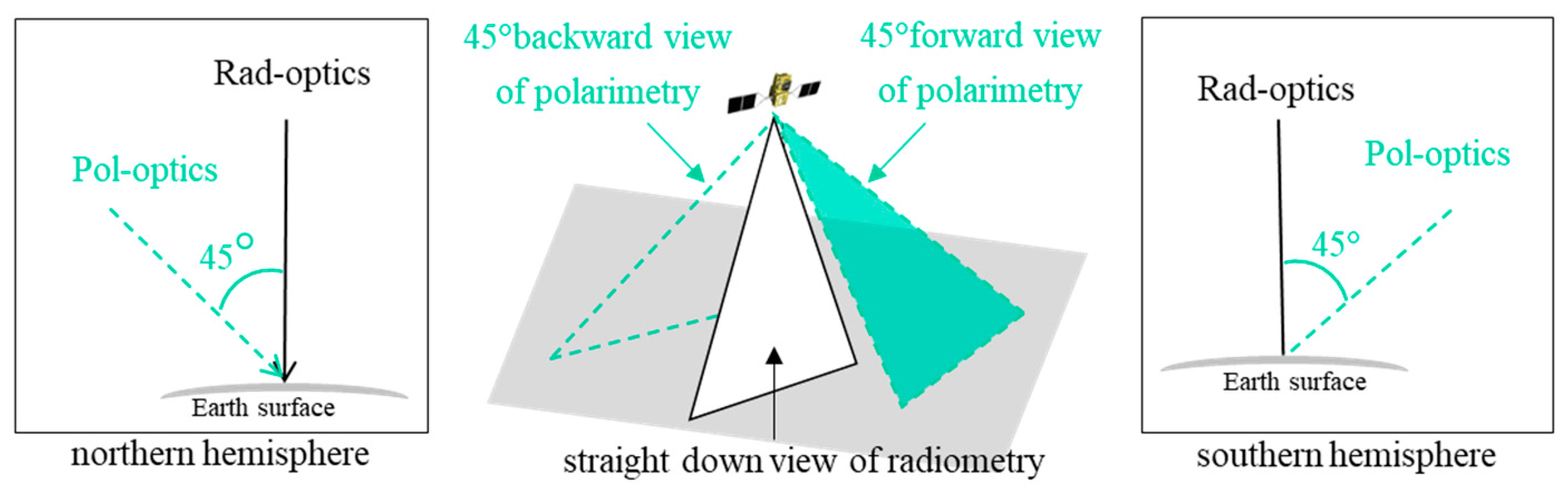
Figure 1. Schematic of SGLI two-directional data acquisition. White and green triangles indicate the line of sight of radiance optics and tilted polarization optics, respectively.
Remotesensing 18 00747 g001
Figure 2. Framework of the regional chemical transport model [35,36].
Remotesensing 18 00747 g002
Figure 3. Schematic of the process for characterizing BBA plumes produced by wildfires.
Remotesensing 18 00747 g003
Figure 4. Color composite images of large-scale forest fires in the northwestern coastal areas of North America on 12–13 September 2020, captured by SGLI at a 250 m resolution.
Remotesensing 18 00747 g004
Figure 5. (a) BBA plume top height estimated from SGLI 2-direction data (partly cited from Hioki et al. 2024 [20]), and (b) vertical profile of BC mass concentration (μg/m3) simulated from CTM.
Remotesensing 18 00747 g005
Figure 6. Characteristics of the BBA retrieved from SGLI data on 13 September 2020. Small squares denote the AERONET/NEON-SJER sites colored by AERONET measurements.
Remotesensing 18 00747 g006
Figure 7. Polarized reflectance (P-ref) at a wavelength of 869 nm in California on 13 September 2020, based on SGLI.
Remotesensing 18 00747 g007
Figure 8. BBA plume images observed by SGLI and GOES on 13 September 2020. (a) 3D topographic map covering 35°N–39°N, 118°W–122°W, (b) SGLI/RGB image at 18:47 on 13 September, (c) GOES/RGB images on 13 September.
Remotesensing 18 00747 g008
Figure 9. Optical properties of atmospheric aerosols retrieved from SGLI polarization and radiance data through radiative transfer calculations. Small black squares denote the AERONET/Jambi site, colored by the daily mean of AERONET measurements as AOT: 3.82 and AE: 1.42. AERONET measurements. (b′) AE distribution in the BBA plume domain.
Remotesensing 18 00747 g009
Figure 10. Concentration of aerosols within the BBA plume area at various altitudes (h) simulated from the CTM on 21 September 2019.
Remotesensing 18 00747 g010
Figure 11. Top height of the BBA plume in Sumatra on 21 September 2019 from SGLI 2-directional data (partly cited from Hioki et al. 2024 [20]). Small red dots denote MODIS/hotspots.
Remotesensing 18 00747 g011
Figure 12. Polarized reflectance (P-ref) at a wavelength of 869 nm in Sumatra on 21 September 2019, based on SGLI. The white dotted line corresponding to the white dotted line in Figure 9b′ indicates regions where the mixing of oceanic aerosols cannot be ignored.
Remotesensing 18 00747 g012
Figure 13. Trends of the averaged AOT (500 nm) and AE values in each BBA plume top height cluster (see Table 1 and Table 2). The value of AOT is colored based on the bottom scale diagram, and the particle size is represented by a gray circle (not to scale).
Remotesensing 18 00747 g013
Table 1. GCOM-C/SGLI channel specification.
ChannelCenter Wavelength (nm)Band Width (nm)Spatial Resolution (m)
Non-polarization Channel138010250 *1
241210
344310
449010
553020
656520
7673.520
8673.520
976312
10868.520
11868.520
Polarization ChannelP1673.5201000
P2868.520
SWI ChannelSW11050201000
SW2138020
SW31630200250 *1
SW42210501000
TIR ChannelT110.8 *20.74 *2250 *3
T212.0 *20.74 *2
*1 Possible to be reduced to 1 km resolution over both polar and ocean regions, except the coastal region. *2 Unit of TIR is micro-meter. *3 Possible to be reduced to 500 m/1 km resolution over both polar and ocean regions, except the coastal region.
Table 2. Averaged AOT (500 nm) and AE values for each BBA plume top height cluster in California on 13 September 2020.
Top Height (h m)AOT (500)AE
6500 h 5.782.10
6000 h < 6500 5.692.04
5000 h < 6000 5.321.77
3000 h < 5000 4.411.74
Table 3. Averaged values of AOT (500 nm) and AE in each BBA plume top height cluster in Sumatra on 21 September 2019.
Top Height (h m)AOT (500)AE
3000 h
2000 h < 3000 5.221.76
1000 h < 2000 5.061.64
0 h < 1000 4.921.46
Disclaimer/Publisher’s Note: The statements, opinions and data contained in all publications are solely those of the individual author(s) and contributor(s) and not of MDPI and/or the editor(s). MDPI and/or the editor(s) disclaim responsibility for any injury to people or property resulting from any ideas, methods, instructions or products referred to in the content.