An Interpretable Nonlinear Intelligent Bias Correction Method for FY-4A/GIIRS Hyperspectral Infrared Brightness Temperatures

Highlights

What are the main findings?

• An intelligent bias correction method integrating ensemble learning and SHAP analysis is proposed for FY-4A/GIIRS brightness temperature data, significantly improving the accuracy of estimating the systematic bias component from observation increments, while enhancing model stability and generalization performance.
• The SHAP interpretability framework is applied to satellite bias correction for the first time, quantitatively revealing the complex nonlinear interaction mechanisms between key forecast predictors and the systematic bias component within observation increments.

What are the implication of the main finding?

• This method generates high-quality bias-corrected brightness temperatures by effectively removing the systematic bias component from observation increments, providing a more reliable data foundation for the assimilation of hyperspectral satellite observation, thus supporting improvements in numerical weather prediction.
• A full-process example of “channel selection, intelligent correction, mechanism interpretation” is established, advancing the explainable and reliable application of artificial intelligence in the meteorological field.

Abstract

The hyperspectral infrared observations of the Geostationary Interferometric Infrared Sounder (GIIRS) on the Fengyun-4A (FY-4A) satellite are an important data source for numerical weather prediction (NWP) assimilation. However, there are systematic differences between observed and simulated brightness temperatures (i.e., the observation increments contain predictable systematic bias components). To address the issue that traditional linear methods struggle to capture the nonlinear relationships between biases and forecast predictors, this study proposes an intelligent bias correction method that integrates ensemble learning and explainable artificial intelligence. First, the entropy reduction method is used to select 69 mid-wave channels. Then, Random Forest, XGBoost, LightGBM, Decision Tree, and Extra Tree are used as base learners to construct a weighted average ensemble model. Training and validation are conducted using high-frequency clear-sky observation data from FY-4A/GIIRS during Typhoon Lekima. The results show that: (1) the ensemble learning correction method outperforms single models and traditional offline methods, with root mean square errors of brightness temperature bias of less than 0.9209 K for the training set and 1.4447 K for the test set; (2) Shapley Additive Explanations (SHAP)-based interpretability analysis reveals the contribution and nonlinear influence mechanisms of factors such as longitude, atmospheric thickness, surface temperature, and total precipitable water on bias correction. This study provides an intelligent bias correction framework with both high precision and explainability, offering a reference for the bias correction and assimilation applications of hyperspectral satellite observations like GIIRS.

1. Introduction

The accuracy of numerical weather prediction (NWP) is highly dependent on the quality of the initial conditions provided by data assimilation systems [1]. Owing to their high spectral resolution and rich information content, hyperspectral infrared satellite observations have become one of the most important data sources for improving forecast skill in modern data assimilation systems [2]. However, there are systematic differences between satellite-observed brightness temperatures and those simulated from the NWP background field. These differences (i.e., the observation increments) contain predictable systematic bias components, which need to be removed during correction. These differences arise from instrument noise, uncertainties in radiative transfer modeling, and representativeness errors [3,4]. To satisfy the assumption of unbiased Gaussian-distributed observation errors in variational data assimilation theory, effective bias correction of satellite observations is essential [5].

Traditional bias correction approaches can generally be classified into “offline” statistical methods [5] and “online” variational bias correction (VarBC) schemes [6], along with their various extensions [7]. Offline methods are computationally efficient but rely on fixed coefficients, making them difficult to adapt to rapidly evolving weather systems. In contrast, online VarBC treats bias correction coefficients as control variables that are optimized simultaneously with atmospheric state variables, thereby offering adaptive capability. Nevertheless, VarBC typically assumes linear or simple parameterized relationships, which limits its ability to accurately represent the complex nonlinear dependencies between biases and forecast-related predictors [7]. In recent years, machine learning techniques have demonstrated considerable potential in bias correction owing to their strong nonlinear fitting capability [8,9]. For example, Random Forest and XGBoost have been applied to the bias correction of brightness temperatures from the Geostationary Interferometric Infrared Sounder (GIIRS) onboard Fengyun-4A (FY-4A), yielding improved performance compared with traditional approaches [10].

However, a single machine learning model may suffer from generalization issues, such as overfitting or underfitting, and its prediction process is often regarded as a “black box” lacking physical interpretability, which limits its further application in operational numerical weather prediction systems that require high reliability. Ensemble learning, by combining the predictions of multiple base learners, can improve model generalization capability and robustness to a certain degree [11,12]. Meanwhile, explainable artificial intelligence techniques, such as Shapley Additive Explanations (SHAP), are capable of quantifying the contribution of each input feature to the model output, thereby enabling a better understanding of the decision-making processes of complex machine learning models [13].

As the world’s first hyperspectral infrared sounder aboard a geostationary satellite, FY-4A/GIIRS plays a crucial role in improving regional and global NWP through its assimilation applications [14,15]. However, the difference between observed and simulated brightness temperatures (i.e., the observation increment) contains systematic bias components, which must be effectively corrected before variational data assimilation [15,16,17]. The objective of this study is to develop a nonlinear intelligent bias correction method for mid-wave infrared channel brightness temperatures from FY-4A/GIIRS by integrating ensemble learning with SHAP-based interpretability analysis. The main components of this study include: (1) optimal selection of GIIRS mid-wave channels using the entropy reduction method [18]; (2) construction of an ensemble learning-based bias corrector with Random Forest [19], XGBoost [12], LightGBM [20], Decision Tree [21], and ExtraTree [22] as base models [23,24]; and (3) analysis of the contributions and nonlinear effects of air-mass-related forecast predictors on bias correction results using the SHAP method [13]. This study aims to enhance bias correction accuracy while simultaneously improving model interpretability and physical credibility.

The remainder of this paper is organized as follows: Section 2 introduces the model and data used in the experiments. Section 3 describes the methods adopted in this study. Section 4 presents the results of bias correction experiments based on FY-4A/GIIRS data. Section 5 provides discussion, conclusions, and future work.

2. Model and Data Preprocessing

2.1. Radiative Transfer Model

In this study, the Radiative Transfer for Tiros Operational Vertical Sounder (RTTOV) model is employed to simulate satellite brightness temperatures. RTTOV enables efficient computation of the radiances received by satellite sensors under given atmospheric conditions [25]. Using the forward operator of RTTOV, top-of-atmosphere radiances for the FY-4A/GIIRS mid-wave infrared channels are calculated based on atmospheric profiles at each field-of-view location and the corresponding satellite observation geometry, and are subsequently converted into channel brightness temperatures via the Planck function [24]. The satellite spectral coefficient files used in the simulations are provided by the National Satellite Meteorological Center (NSMC).

2.2. Data

2.2.1. FY-4A/GIIRS Data

FY-4A/GIIRS is the world’s first hyperspectral infrared atmospheric vertical sounder onboard a geostationary satellite. It adopts a multidimensional array sensor architecture (32 × 4 elements) combined with Fourier transform spectrometry, and achieves regional coverage through a step-and-stare scanning method: the scanning mirror steps in the east–west direction, dwelling on each field of view for approximately 1.5 s to acquire an interferogram, and then steps to the next position. After completing a row of east–west scans, the scanning mirror steps in the north–south direction to begin the next row of scans [14,16,26]. It provides dual-band observations in the long-wave infrared (700–1130 cm⁻¹, 689 channels) and mid-wave infrared (1650–2250 cm⁻¹, 961 channels) regions, with a spatial resolution of 16 km at the nadir point [14,27]. Its high temporal resolution observation capability provides high-frequency regional observation data for numerical weather prediction. Assimilation of FY-4A/GIIRS data is therefore of great importance for improving the accuracy of initial conditions and enhancing forecasts of typhoon tracks and precipitation. The Level-1 brightness temperature radiance data used in this study are obtained from the official website of the National Satellite Meteorological Center (NSMC).

2.2.2. Cloud Mask Product

In this study, a 4 km resolution cloud mask product (CLM) derived from the Advanced Geosynchronous Radiation Imager (AGRI) onboard FY-4A is used to identify clear-sky fields of view [28]. The AGRI cloud mask results are spatially and temporally collocated with GIIRS fields of view to calculate the cloud fraction for each pixel [24,29]. Fields of view with a cloud fraction equal to zero are defined as “absolutely clear-sky” pixels and are subsequently used for bias correction experiments.

2.2.3. Background Fields and Simulated Brightness Temperatures

The background atmospheric profiles are obtained from the Final Global Data Assimilation System (FNL) analysis fields produced by the National Centers for Environmental Prediction (NCEP) [9]. The spatiotemporal matching method between the background field NCEP/FNL and FY-4A/GIIRS observations is as follows: For temporal matching, the FNL analysis time closest to the GIIRS observation time is selected (within ±3 h), and linear interpolation is applied to match the observation time. For spatial matching, the FNL grid field is interpolated to the longitude and latitude positions of the GIIRS fields of view using bilinear interpolation. Subsequently, the RTTOV model, along with the satellite spectral coefficient file, is used to simulate the brightness temperatures of each channel based on the interpolated background field.

2.2.4. Data Preprocessing and Experimental Setup

The study period spans from 20:00 UTC on 8 August to 11:00 UTC on 10 August 2019, corresponding to the high-frequency observation phase of Typhoon Lekima. The study domain covers 98°E–160°E and 12°N–49°N [24]. The data preprocessing procedures include: (1) apodization and spectral smoothing applied to GIIRS observations [16,24,30]; (2) spatial and temporal collocation with the AGRI cloud mask product to identify “absolutely clear-sky” fields of view; and (3) rough quality control performed on the observed and simulated brightness temperatures to remove physically unrealistic values, specifically excluding data above 300 K or below 150 K. This range is consistent with the dynamic range of the GIIRS instrument and the expected physical limits of Earth’s emitted infrared radiation [31]. After preprocessing, the full dataset is randomly divided into a training set (80%) for model training and hyperparameter optimization and an independent test set (20%) for final evaluation [32].

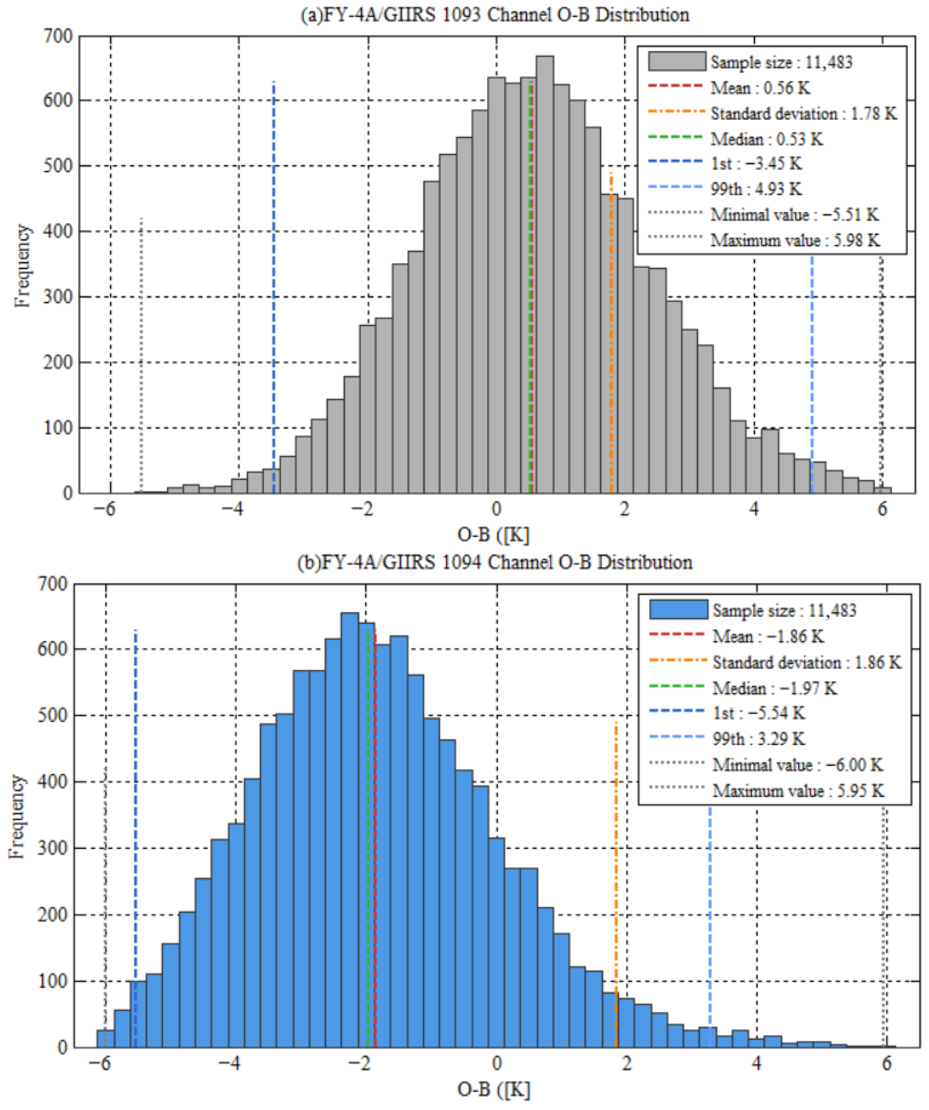
This study uses representative channels 1093 and 1094 as examples to analyze the distribution characteristics of the difference between observed brightness temperature (O) and simulated brightness temperature (B) (O-B). Channels 1093 and 1094 are selected for analysis based on the following considerations: the peak of the weighting function for channel 1094 is located at 703.6 hPa (lower-middle troposphere), a height that is highly sensitive to temperature and water vapor distribution; and channel 1093 is adjacent in spectral position to channel 1094, with the peak of its weighting function at 661.0 hPa. The O-B statistical characteristics of the two channels show significant differences—channel 1093 exhibits a positive bias (mean 0.56 K), while channel 1094 exhibits a negative bias (mean −1.86 K). The selection of these two channels allows for testing the consistency of the proposed correction method across different bias directions.

Figure 1 shows that the O-B values of channels 1093 and 1094 deviate from a Gaussian distribution. For channel 1093, the mean O-B is 0.56 K, with a standard deviation of 1.78 K, and the 1st–99th percentile range is [−3.45 K, 4.93 K]. The maximum and minimum O-B values are 5.98 K and −5.51 K, respectively. For channel 1094, the mean O-B is −1.86 K, with a standard deviation of 1.86 K, and the 1st–99th percentile range is [−5.54 K, 3.29 K]. The maximum and minimum O-B values are 5.95 K and −6.00 K, respectively. To fully preserve the nonlinear variation characteristics of the bias and avoid losing effective training samples due to hard threshold truncation, no explicit O-B removal threshold was set during the preprocessing. The potential impact of extreme O-B outliers on model training is discussed in Section 5.

It should be noted that, in designing the dataset size and data partitioning strategy, this study follows sample configurations adopted in related studies. Cai et al. used FY-4A/GIIRS observations with 4018 training samples and 2678 test samples to conduct temperature and humidity profile retrievals [33]. Malmgren-Hansen et al. performed temperature profile retrievals based on single-day Infrared Atmospheric Sounding Interferometer (IASI) data [34]. Furthermore, inspired by the approach of Ma et al. [27], which utilized high-frequency FY-4A/GIIRS observations during Typhoon Maria, this study selects high-frequency clear-sky fields of view during Typhoon Lekima to construct a dataset comprising a total of 11,483 fields of view. After proportional partitioning, the training set contains 9186 fields of view for model training and hyperparameter tuning, while the test set includes 2297 fields of view for independent validation and performance evaluation.

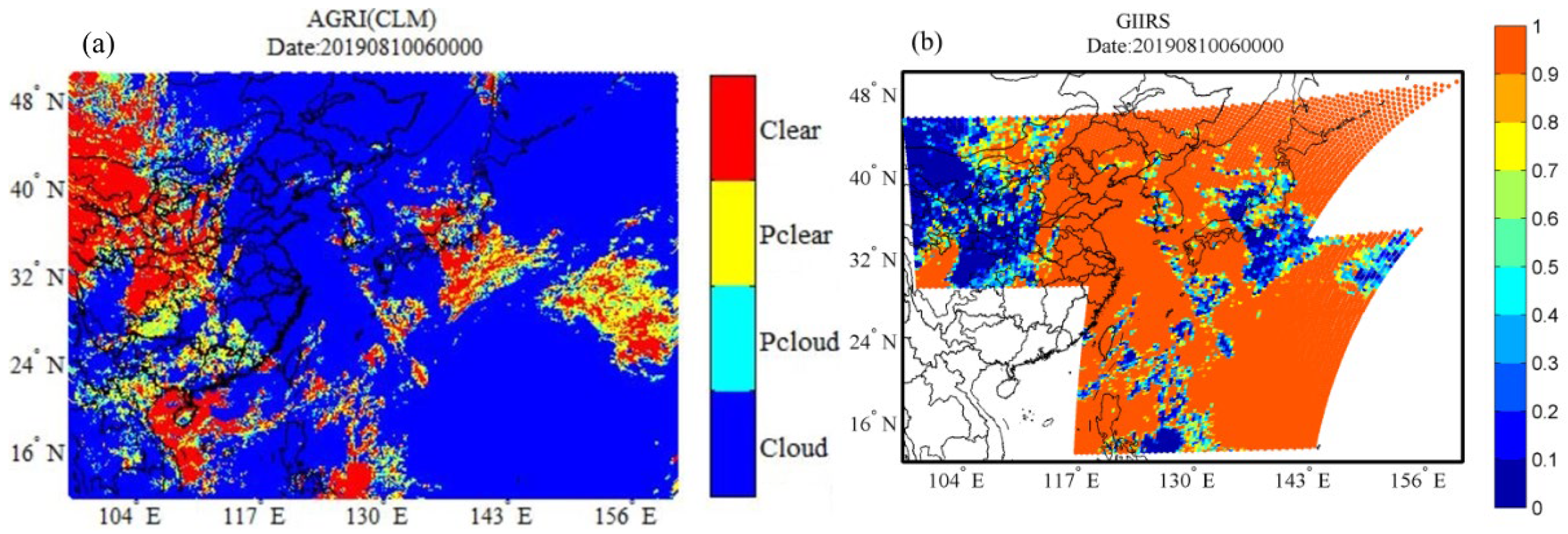
The spatial distribution of cloud fraction over the study region is shown in Figure 2 for 06:00 UTC on 10 August 2019. Figure 2a presents the original AGRI cloud mask product (CLM), which includes four categories: Cloudy, Probably Cloudy (Pcloud), Probably Clear (Pclear), and Clear [28]. Figure 2b shows the cloud fraction distribution at the GIIRS fields of view, where a cloud fraction of zero denotes absolutely clear-sky conditions, and warmer colors indicate larger cloud fractions. Within the high-frequency observation region, both clear-sky and cloudy fields of view are widely distributed, while transitional states (probably clear/probably cloudy) are mainly located along the boundaries between the two.

3. Methods

3.1. Problem Definition

For a given FY-4A/GIIRS channel, the difference (O-B) between the observed brightness temperature (O) and the background field simulated brightness temperature (B) is defined as the observation increment, which can be expressed as:

$$y-H\left(x_b\right)=\left[y-H\left(x_t\right)\right]+\left[H\left(x_t\right)-H\left(x_b\right)\right]$$

(1)

In this equation, $y$ represents the observed brightness temperature, $x_t$ denotes the true atmospheric state, $x_b$ is the background field, and $H$ is the radiative transfer model. $H\left(x_b\right)$ is the simulated brightness temperature. The observation increment contains contributions from the following components: (1) observation errors (e.g., instrument noise); (2) forward model errors (uncertainties in the radiative transfer model); (3) differences between the background field and the true atmospheric state. The goal of bias correction is to estimate and remove the systematic bias components (i.e., the predictable part caused by instrument biases, model biases, etc.) from the observation increment, so that the corrected observed brightness temperature is as close as possible to the unbiased simulated value $H\left(x_t\right)$ [5,35].

This study establishes a nonlinear mapping relationship between the set of forecast predictors $x\in {ℝ}^d$ and the systematic bias components in the observation increment (O-B).

$$\widehat{b}\left(x\right)=f\left(x\right)+ϵ$$

(2)

Here, $\widehat{b}\left(x\right)$ represents the estimated systematic bias, $f\left(\cdot \right)$ refers to the ensemble learning model and base models, and $ϵ$ represents the residual random error. Commonly used forecast predictors $x$ include the 1000–300 hPa thickness, the 200–50 hPa thickness, model surface temperature, total column water vapor, and the longitude and latitude of the field-of-view (FOV) pixel [10,36].

It should be noted that this study focuses on the implementation of the offline method by Harris and Kelly [5] for correcting air mass biases, without separately considering the latitude dependence of scan angle biases. The reason is that: FY-4A/GIIRS is a geostationary satellite, and its scan angle is implicitly related to the field of view’s latitude and longitude, which have already been incorporated as forecast predictors in the machine learning model. Moreover, the core objective of this study is to compare nonlinear correction based on forecast predictors with traditional linear correction methods.

3.2. Base Machine Learning Models

In this study, five tree-based machine learning algorithms are selected as base learners:

(1) Random Forest (RF): An ensemble method that constructs multiple decision trees and aggregates their predictions, enhancing generalization performance through out-of-bag sample evaluation and feature randomness [19].

(2) Extreme Gradient Boosting (XGBoost): An efficient gradient boosting framework that sequentially builds decision trees to minimize a loss function, while incorporating regularization terms to prevent overfitting [12].

(3) Light Gradient Boosting Machine (LightGBM): Utilizes histogram-based decision tree algorithms and a leaf-wise growth strategy to significantly improve training speed and reduce memory consumption, making it suitable for large-scale data processing [20].

(4) Decision Tree (DT): A nonparametric supervised learning model that performs prediction or classification by recursively partitioning the data into increasingly homogeneous subsets [21].

(5) Extremely Randomized Trees (Extra Trees): An ensemble tree-based method that introduces stronger randomness by selecting split features and thresholds entirely at random at each node, thereby further reducing model variance and improving generalization performance [22].

3.3. Ensemble Learning Strategy

To integrate the strengths of the individual base models, a weighted averaging ensemble strategy is adopted [23,24]. The integrated prediction of the systematic bias component in the observation increment is expressed as:

$${\widehat{b}}_{ens}\left(x\right)={\displaystyle \sum _{i=1}^M{w}_i·}{f}_i\left(x\right)$$

(3)

Here, $M$ denotes the number of base models, and $f_i$ and $w_i$ represent the prediction of the systematic bias component by the $i$-th base model and its corresponding ensemble weight ($w_i\ge 0$, ${\displaystyle \sum _{i=1}^M{w}_i}=1$). The weights are determined by optimizing the ensemble prediction (i.e., minimizing the mean squared error), enabling the ensemble model to more accurately estimate the systematic bias component in the observation increment.

3.4. Base Model Configuration

To enhance the model’s generalization ability on independent samples and avoid the overfitting or underfitting risks that may occur with a single model, this study adopts a weighted average ensemble strategy to integrate the predictive advantages of multiple base models. Before constructing the ensemble model, the hyperparameters of the five base models are first optimized. The key hyperparameters of each base model are optimized using a grid search combined with cross-validation, while other parameters are kept at their default settings. The optimized hyperparameters include:

• RF: number of trees (n_estimators), maximum tree depth (max_depth).
• XGBoost: n_estimators, max_depth, learning rate, and the minimum loss reduction threshold (gamma).
• LightGBM: learning rate, number of leaves (num_leaves), and n_estimators.
• Decision Tree: max_depth, minimum number of samples required at a leaf node (min_samples_leaf), and the minimum number of samples required to split an internal node (min_samples_split).
• Extra Tree: max_depth, min_samples_leaf, min_samples_split.

After the above hyperparameter optimization is completed, each base model will participate in the subsequent weighted average ensemble learning modeling with the optimal configuration.

3.5. SHAP-Based Interpretability Analysis

SHAP values are used to quantify the contribution of each forecast predictor $x$ to an individual prediction $\delta {\widehat{T}}_b$. Grounded in Shapley values from cooperative game theory, SHAP provides a unified and consistent measure of feature importance for the model. For the $j$-th feature, its SHAP value ${\varphi }_j$ represents the contribution of that feature to a specific prediction relative to the mean prediction. The model prediction can be expressed as the sum of the SHAP values of all features plus the base value (i.e., the average prediction over all samples) [13,37]:

$$f\left(x\right)={\varphi }_0+{\displaystyle \sum _{j=1}^d{\varphi }_j\left(x\right)}$$

(4)

Here, ${\varphi }_0$ denotes the base value, and ${\varphi }_j$ represents the SHAP value of the $j$-th feature. By analyzing the distributions and dependence plots of SHAP values, it is possible to understand how each forecast predictor influences the bias correction results, as well as the extent and nature of its impact (linear or nonlinear).

3.6. Optimal Selection of GIIRS Mid-Wave Channels Based on the Entropy Reduction Method

Following the study of [18], the entropy reduction (ER) method is employed to evaluate the contribution of individual channels to the analysis error covariance, and 69 information-rich channels are optimally selected from the GIIRS mid-wave infrared channels. The channel selection aims to maximize the information gain of the selected channel subset under a given constraint on the number of channels [38,39].

Let the information entropy reduction after the $k$-th iteration be denoted as $E{R}_k$, which is defined as:

$$E{R}_k={\displaystyle \frac{1}{2}}\ln \left[\det \left(S_k{B}^{-1}\right)\right]$$

(5)

Here, $S_k$ denotes the analysis error covariance matrix updated at the $k$-th iteration, and $B$ represents the background error covariance matrix. The iterative update of $S_k$ is given by:

$$S_k=S_{k-1}\left[I-{\displaystyle \frac{h_k{\left(S_{k-1}{h}_k\right)}^T}{r_k+{\left(S_{k-1}{h}_k\right)}^T{h}_k}}\right]$$

(6)

Here, $h_k$ denotes the normalized Jacobian matrix of the $k$-th channel [40], and the initial value of $S_0$ is set to $B$. $I$ represents the identity matrix, and $r_k$ denotes the observation error standard deviation of the $k$-th channel. The detailed computational procedure is described in Wang et al. [18].

3.7. Accuracy Evaluation Methods

Following the methodology of [9], the objective of this study is likewise to make the bias-corrected satellite-observed brightness temperatures closer to the values simulated by the radiative transfer model. The Pearson correlation coefficient (CC) and the root mean square error (RMSE) are employed to evaluate the performance of bias correction. The CC is defined as:

$$\mathrm{CC}={\displaystyle \frac{{\displaystyle \sum _{k=1}^n\left(F_k-\overline{F}\right)\left(T_k-\overline{T}\right)}}{\sqrt{{\displaystyle \sum _{k=1}^n{\left(F_k-\overline{F}\right)}^2}}\sqrt{{\displaystyle \sum _{k=1}^n{\left(T_k-\overline{T}\right)}^2}}}}$$

(7)

The RMSE is defined as:

$$\mathrm{RMSE}=\sqrt{{\displaystyle \frac{1}{n}}{\displaystyle \sum _{k=1}^n{\left(F_k-T_k\right)}^2}}$$

(8)

Here, $n$ denotes the number of samples. $F_k$ and $T_k$ represent the bias-corrected brightness temperatures from FY-4A/GIIRS and the simulated brightness temperatures, respectively, while $\overline{F}$ and $\overline{T}$ denote their corresponding mean values.

4. Results

4.1. Channel Selection Experiment Based on the Entropy Reduction Method

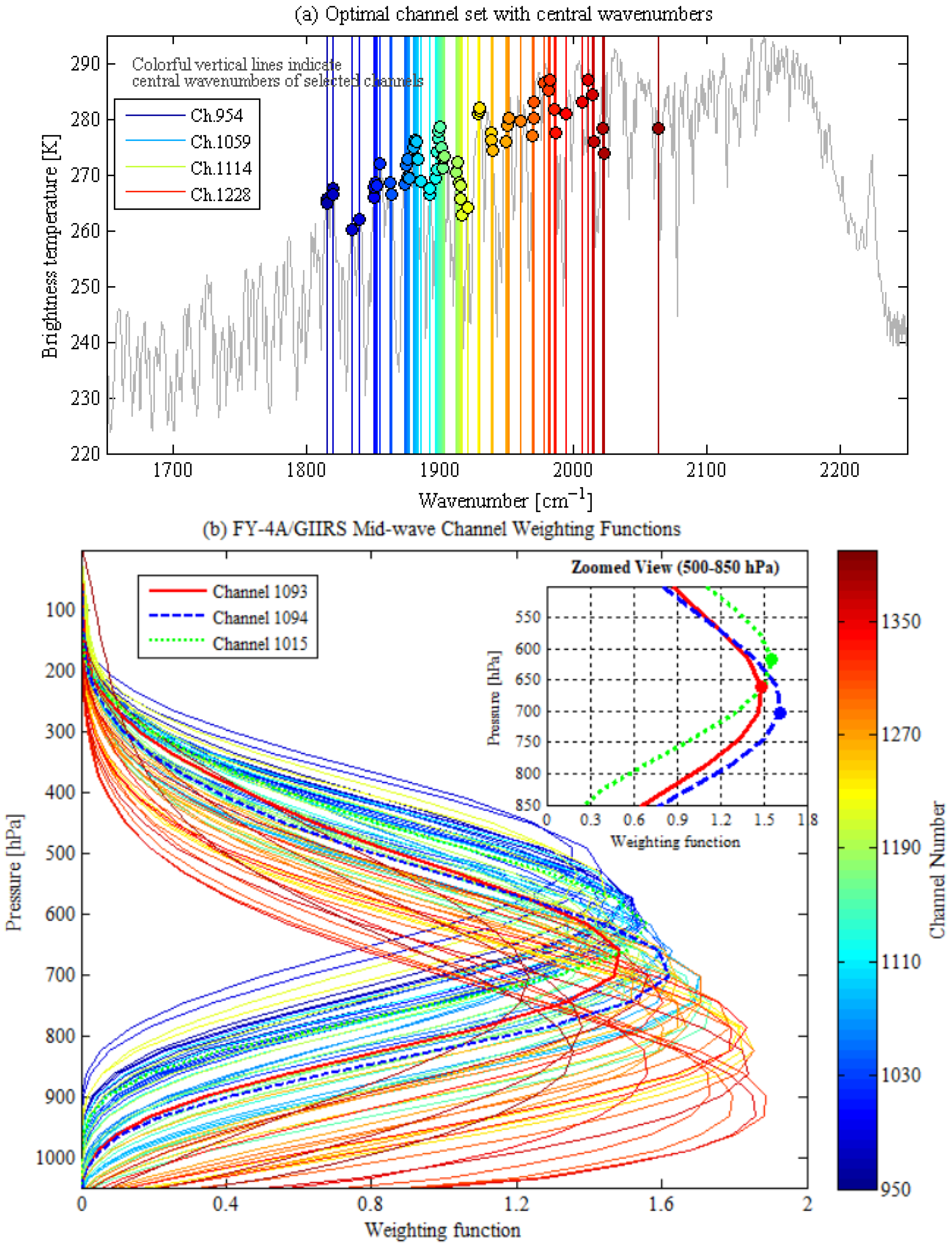
Using the entropy reduction method, 69 relatively information-rich channels are optimally selected from the FY-4A/GIIRS mid-wave infrared band. The peaks of the weighting function for the selected channels are primarily distributed from the lower to the middle-upper levels of the troposphere. This vertical coverage ensures that the selected channels are representative of the tropospheric thermal structure. Owing to the presence of overlapping weighting function peaks among hyperspectral channels, an “overdetermined” characteristic exists in the vertical dimension, which makes channel selection necessary [1,18].

Figure 3a shows the spectral positions of the 69 GIIRS mid-wave channels selected using the entropy reduction method, while Figure 3b presents the vertical distributions of the weighting functions for these channels. Simulated brightness temperatures for FY-4A/GIIRS channels (grey line) in Figure 3a and the weighting functions in Figure 3b are calculated using the RTTOV model with a standard midlatitude atmospheric profile. In Figure 3a, the colored vertical lines indicate the central wavenumber positions of the selected channels. In Figure 3b, the distribution of the weighting functions for the selected channels is shown, with colors ranging from blue to red representing the increasing channel numbers. The weighting functions are not normalized and are presented solely to provide a qualitative visualization of the vertical sensitivity characteristics of each channel. To clearly highlight the channels 1093, 1094, and 1015, which are the focus of this study, Figure 3b shows these three channels in bold and presents an enlarged inset displaying the shape of the weighting function peaks for these channels.

4.2. Bias Correction Experiment Based on Ensemble Learning

4.2.1. Experimental Setup and Procedure

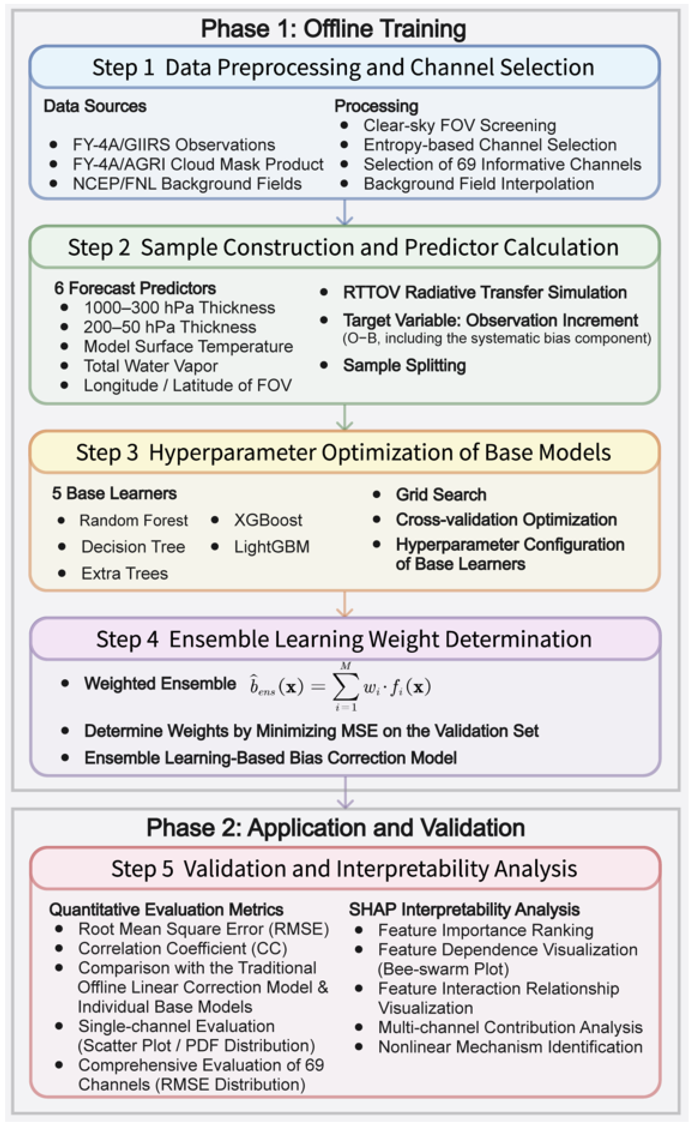
In this study, the FY-4A/GIIRS clear-sky fields of view data during the high-frequency observation period of Typhoon Lekima (from 8 to 10 August 2019) are selected to conduct bias correction experiments for mid-wave channel brightness temperatures. The experiment adopts an “offline” training-application model, which consists of the following five steps:

(1) Data Preprocessing and Channel Selection: Clear-sky GIIRS fields of view are selected based on the FY-4A/AGRI cloud mask product. Then, the entropy reduction method is applied to select 69 information-rich channels from the GIIRS mid-wave band. Meanwhile, NCEP/FNL analysis field background data is interpolated to the GIIRS fields of view locations.

(2) Sample Preparation and Forecast Predictor Calculation: Using the RTTOV radiative transfer model, the brightness temperatures of the selected channels are simulated based on the interpolated FNL background field. For each clear-sky field of view, the corresponding air-mass-related forecast predictors are calculated, including: 1000–300 hPa thickness, 200–50 hPa thickness, model surface temperature, total water vapor, and the longitude and latitude of the field of view. Finally, using the forecast predictors as input and the systematic bias component in the difference between observed and simulated brightness temperatures (i.e., the observation increment) is set as the learning target, and the training sample set is constructed.

(3) Hyperparameter Optimization of Base Models: Based on the constructed training sample set, grid search combined with cross-validation is employed to optimize the key hyperparameters of five base machine learning models: Random Forest, XGBoost, LightGBM, Decision Tree, and Extra Trees. This ensures the optimal configuration for each base model.

(4) Determination of Ensemble Learning Weights: On an independent validation set, the optimal weights of each tuned base model in the weighted averaging ensemble strategy are determined by minimizing the mean squared error (MSE) using an optimization algorithm. This results in the construction of the final ensemble learning bias correction model.

(5) Validation and Interpretability Analysis: The performance of the ensemble learning model, each individual base model, and the traditional “offline” linear correction method is evaluated, with the primary evaluation metrics being root mean square error (RMSE) and correlation coefficient (CC). Additionally, SHAP interpretability analysis is applied to diagnose the best-performing ensemble learning model to reveal the contribution of each forecast predictor to the bias correction results and their nonlinear effects.

Steps 1 through 4 constitute the “offline training” phase, which is used to generate the trained models, while Step 5 represents the “application and validation” phase, aiming to assess the model’s generalization ability and interpret its physical mechanisms. These five steps comprehensively cover the entire process from data preparation, model construction, optimization to performance verification and mechanism analysis.

Figure 4 illustrates the complete process of the proposed FY-4A/GIIRS mid-wave infrared channel brightness temperature bias correction method. The model uses the observation increment (O-B, which includes observation errors, forward model errors, and the difference between the background field and the true atmospheric state) as the target variable and estimates the systematic bias component through ensemble learning to achieve bias correction.

4.2.2. Hyperparameter Optimization

Hyperparameter optimization is a critical step to ensure model performance and generalization capability. The hyperparameters of the base models are optimized using grid search combined with cross-validation. The optimal hyperparameter settings are as follows:

• RF: n_estimators = 31, max_depth = 15.
• XGBoost: max_depth = 10, learning_rate = 0.5, n_estimators = 32, gamma = 3.
• LightGBM: learning_rate = 0.2, num_leaves = 60, n_estimators = 90.
• Decision Tree: max_depth = 10, min_samples_leaf = 3, min_samples_split = 5.
• Extra Tree: max_depth = 10, min_samples_leaf = 3, min_samples_split = 5.

4.2.3. Results Comparison and Analysis

(1) Single Channel Correction Performance

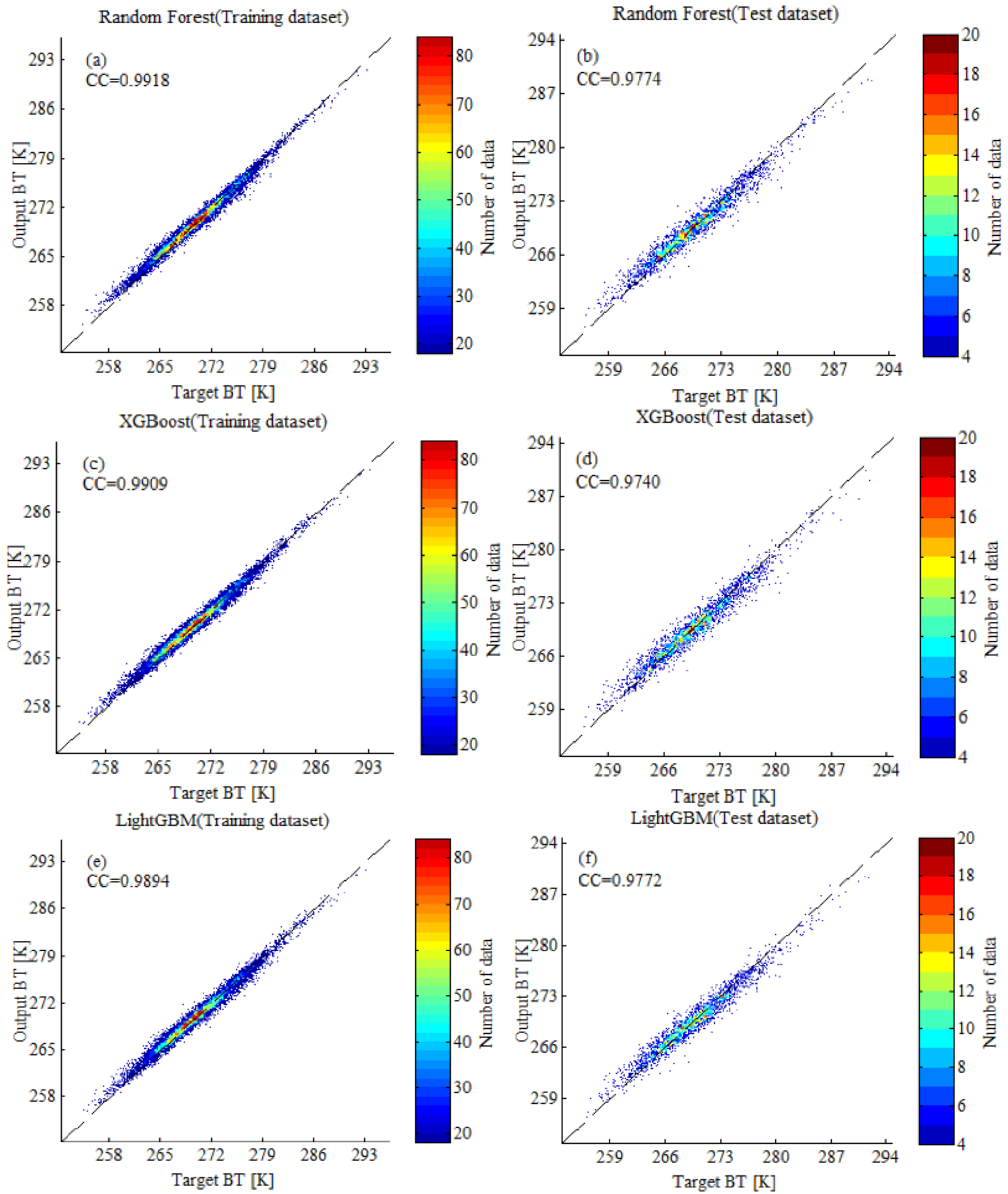
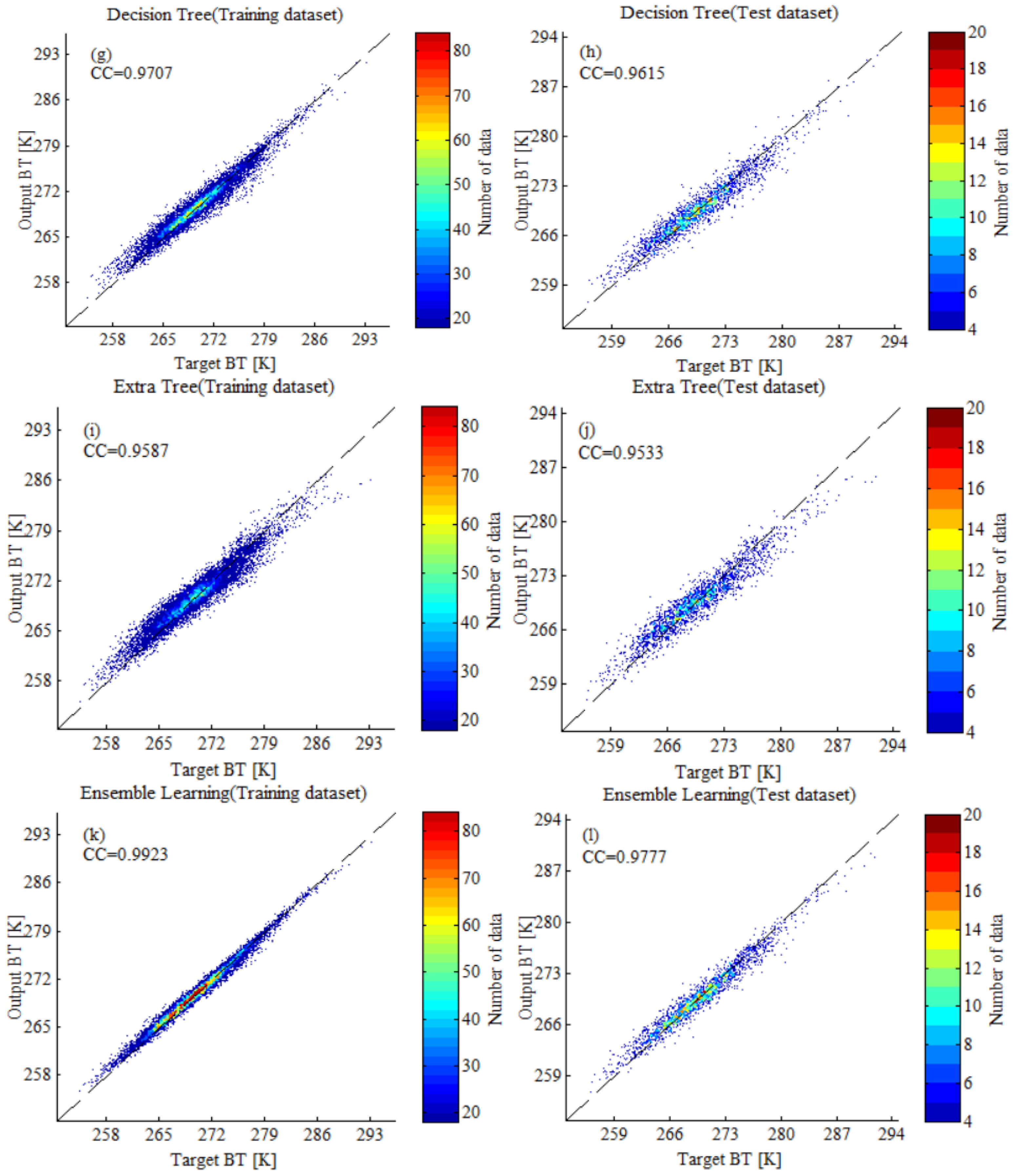
Taking FY-4A/GIIRS channel 1094 as an example, Figure 5 shows scatter plots of the bias correction results for different models on both the training and test datasets. The x-axis represents the target brightness temperature (simulated values), while the y-axis represents the output brightness temperature (corrected observed values). The correlation coefficients for all models exceed 0.95 on both the training and test datasets, indicating that the models have learned certain patterns. The ensemble learning model’s predicted points are more concentrated along the diagonal in the scatter plot, demonstrating relatively better correction performance. In terms of performance, the models are ranked in descending order as follows: Random Forest, XGBoost, LightGBM, Decision Tree, and Extra Tree.

(2) Bias Distribution Changes

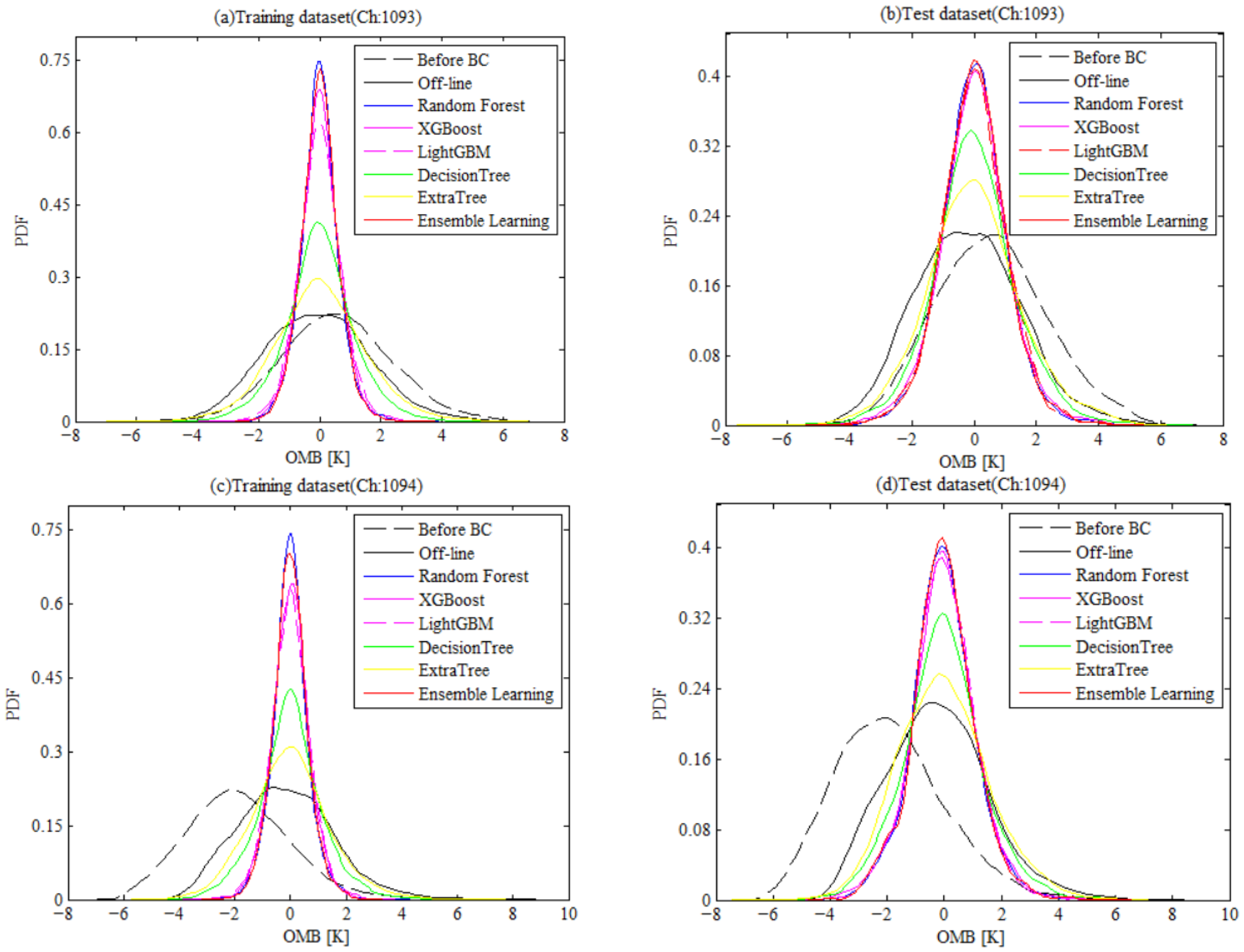
Figure 6 shows the probability density function (PDF) distributions of the brightness temperature biases for FY-4A/GIIRS channels 1093 and 1094 before and after bias correction. Before correction, the bias distributions are relatively scattered. After correction, the bias PDFs for all methods are concentrated around zero, and approximate a Gaussian distribution. The ensemble learning model results in a more concentrated bias distribution. Bias correction was performed using Harris and Kelly’s offline method, as well as Random Forest, XGBoost, LightGBM, Decision Tree, Extra Tree, and the ensemble learning model.

(3) Ensemble Weight Analysis

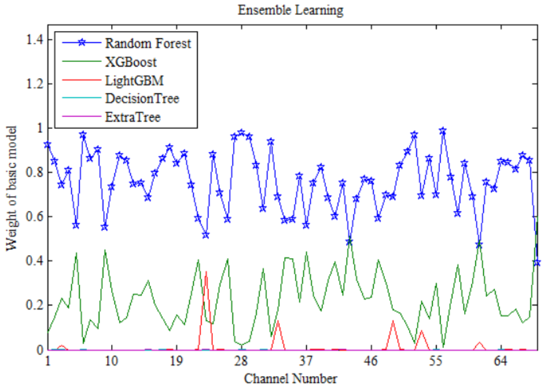
Figure 7 shows the weight distribution of each base model in the ensemble learning model: Random Forest (blue line), XGBoost (dark green line), LightGBM (red line), Decision Tree (light green line), and Extra Tree (magenta line). As can be seen from the figure, the weights of Decision Tree and Extra Tree are zero for certain channels. LightGBM exhibits relatively large weights for a few channels, while its weights tend to zero for most other channels. The ensemble weight for Random Forest is the largest, followed by XGBoost, which corresponds to the relatively better performance of RF on most channels. This indicates that the ensemble model adaptively assigns higher weights to base models with better performance.

(4) Multi-Channel Comprehensive Evaluation

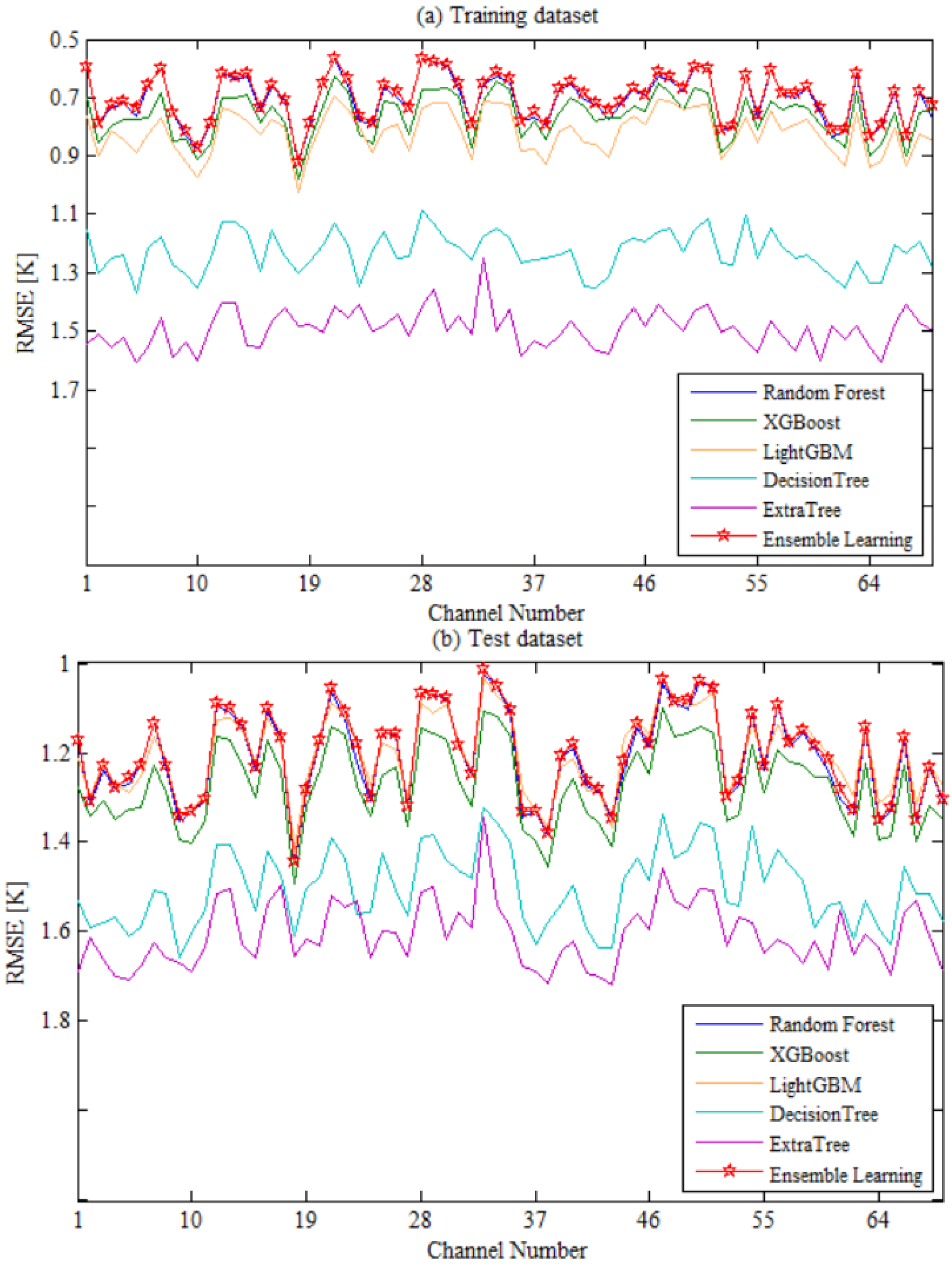
Figure 8 summarizes the RMSE between the corrected observed brightness temperatures and the simulated brightness temperatures for the 69 selected mid-wave channels after correction by different models. The ensemble learning model achieved the smallest average RMSE on both the training and test datasets (with the maximum RMSE of 0.9209 K on the training set and 1.4447 K on the test dataset), further validating its optimal overall correction performance and good generalization ability. The performance ranking of the models on the test dataset is approximately as follows: Ensemble Learning outperforms Random Forest, which outperforms XGBoost, followed by LightGBM, Decision Tree, and Extra Tree in descending order. It should be noted that the GIIRS mid-wave channel brightness temperature biases are generally large, with strong nonlinearity, making correction relatively difficult [10].

Furthermore,

Table 1. Statistics of the RMSE between bias-corrected brightness temperatures and simulated brightness temperatures for different models (unit: K).

Model	Training Dataset (RMSE)		Test Dataset (RMSE)
	Max	Min	Max	Min
Random Forest	0.9214	0.5639	1.4484	1.0251
XGBoost	0.9768	0.6272	1.4937	1.0985
LightGBM	1.0217	0.6932	1.4115	1.0311
Decision Tree	1.3676	1.0859	1.6569	1.3230
Extra Tree	1.6090	1.2497	1.7173	1.3444
Ensemble Learning	0.9209	0.5639	1.4447	1.0140

presents the RMSE between the corrected brightness temperatures and the simulated brightness temperatures for different models in this case study. The maximum (Max) and minimum (Min) RMSE values for the 69 channels are provided separately for the training dataset and the test dataset.

As shown in Table 1, the ensemble learning model achieves both the maximum RMSE (0.9209 K) and minimum RMSE (0.5639 K) on the training set, which are better than or equal to the best performances of the base models, indicating its ability to effectively integrate the advantages of multiple base models. On the test set, the ensemble learning model’s minimum RMSE (1.0140 K) outperforms all single models (with the next best Random Forest showing a reduction of 0.0111 K, from 1.0251 K). The maximum RMSE (1.4447 K) is better than the other four models, except for LightGBM (1.4115 K). Overall, the ensemble learning model achieved the most balanced correction performance on the test set, with the optimal minimum RMSE and a suboptimal maximum RMSE, validating the effectiveness of the weighted average strategy in enhancing model generalization ability and stability.

It should be noted that: This study serves as a feasibility exploration of applying ensemble learning to bias correction. For some models (e.g., Decision Tree and Extra Tree), relatively large RMSE values still occur for certain channels, which could be further reduced in future work through variational minimization within data assimilation systems.

4.3. SHAP-Based Interpretability Analysis of Forecast Predictors

To clearly reveal the influence and relative importance of different features on brightness temperature bias correction, SHAP is employed to analyze the key forecast predictors.

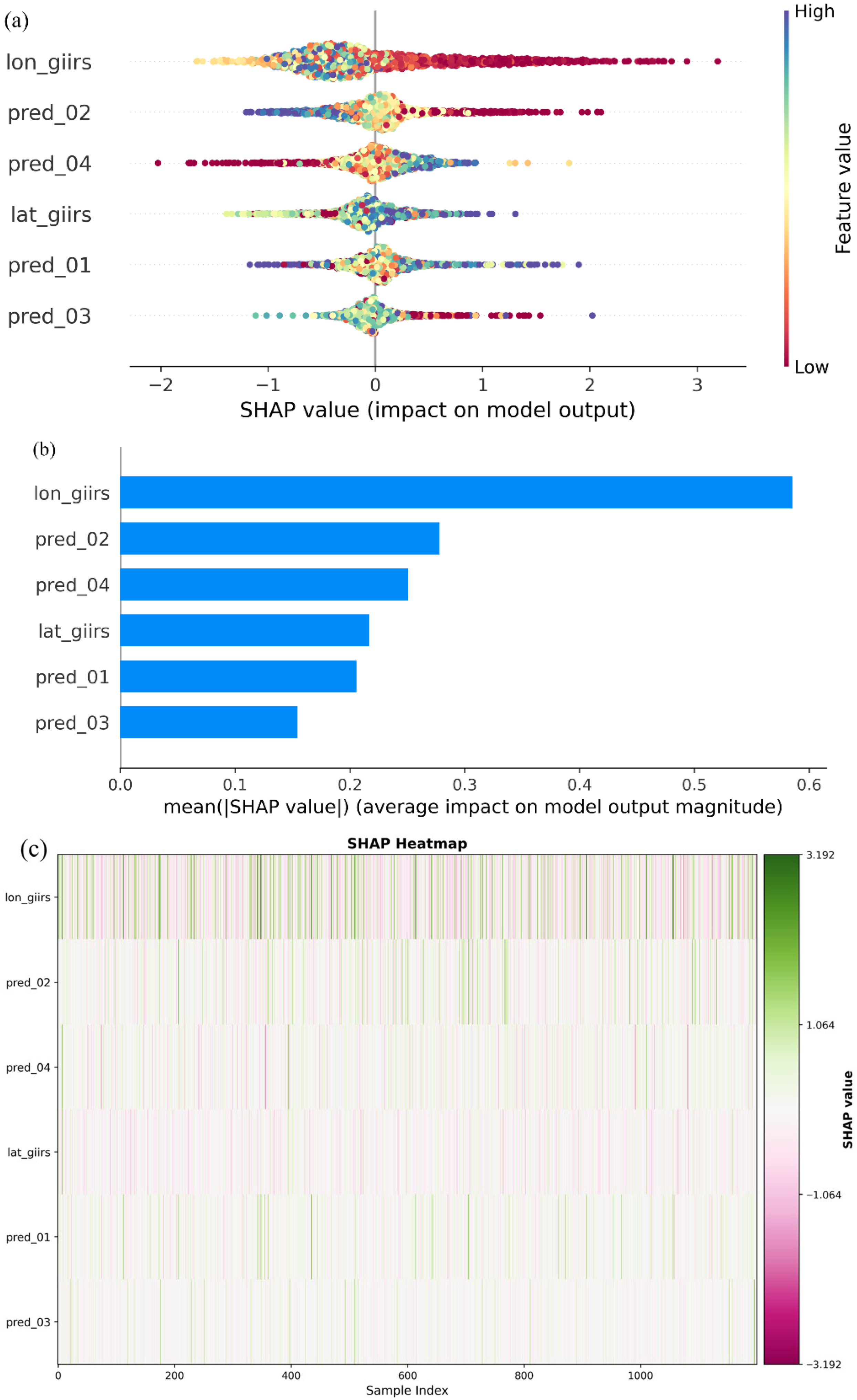
Figure 9 presents the feature density scatter plot (a), feature importance ranking (b), and the heatmap of model outputs (c) for the bias correction of FY-4A/GIIRS channel 1094. It should be noted that, in Figure 9a, the beeswarm summary plot illustrates the relationship between the feature variables (vertical axis) and the corresponding SHAP values for the test dataset (horizontal axis). Each horizontal row represents one feature, while the color scale indicates the magnitude of the feature values, with red denoting low values and blue denoting high values. In this study, the model prediction target is the bias between observed and simulated brightness temperatures (O-B). Therefore, if the SHAP value of a feature is positive, it indicates that the feature pushes the predicted O-B bias value higher (i.e., increases the correction amount); if the SHAP value is negative, it indicates that the feature pushes the predicted O-B bias value lower (i.e., decreases the correction amount). Specifically, “pred_01” represents the 1000–300 hPa thickness, “pred_02” the 200–50 hPa thickness, “pred_03” the model surface temperature, “pred_04” the total column water vapor, “lon_giirs” the longitude of the GIIRS field of view, and “lat_giirs” the latitude.

An analysis of Figure 9a–c indicates that the importance of variables affecting the estimation of systematic bias components in the FY-4A/GIIRS channel 1094 observed brightness temperature increments, in descending order, is as follows: the most influential is the longitude of the field of view, followed by 200–50 hPa thickness, total column water vapor, latitude of the field of view, 1000–300 hPa thickness, and model surface temperature. This ranking indicates that, in the case of Typhoon Lekima studied here, the geographic coordinates (especially longitude) are the primary source of systematic bias causing differences between observed brightness temperatures and background field simulations.

It is worth noting that for channel 1094, with a peak at 703.6 hPa, its bias correction is most dependent on the upper-level thermal factor pred_02 (200–50 hPa thickness), rather than the lower-level thickness factor pred_01, which directly corresponds to the sensitive layer of its weighting function. This phenomenon reveals that, in the case of Typhoon Lekima, the brightness temperature bias of the mid-lower level channels may be systematically modulated by upper-atmosphere dynamic and thermal processes, reflecting the contribution of vertical coupling at weather scales to bias formation. It also highlights the unique value of this intelligent method in identifying complex, cross-layer error associations.

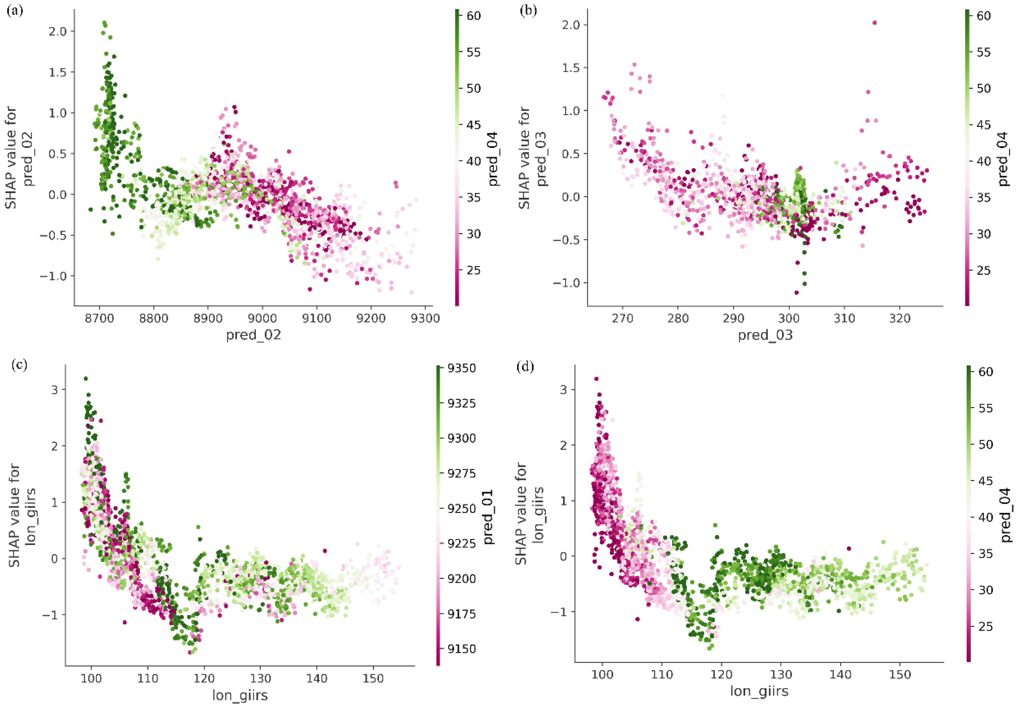
Further, Figure 10 shows the interaction relationships between different variables. Only the relationships between some feature variables (forecast predictors) are presented. The relationships between different features exhibit “nonlinear” characteristics.

As shown in Figure 10, there are complex interactions between the forecast predictors. For example, Figure 10c demonstrates that at different latitudes and longitudes, the contribution of “1000–300 hPa thickness” (lower-level thermal structure) to the brightness temperature bias varies, reflecting the combined impact of the spatial distribution of atmospheric circulation and thermal structure on the bias. Figure 10d illustrates that the magnitude and direction of the impact of longitude on the bias change under different total column water vapor conditions. This suggests that the distribution of water vapor and geographic factors jointly influence the radiative transfer process. The existence of these nonlinear interactions explains why simple linear regression models, based on physical understanding, fail to fully capture the complexity of the biases, while machine learning models (such as tree-based models) that can represent these relationships perform better in bias correction.

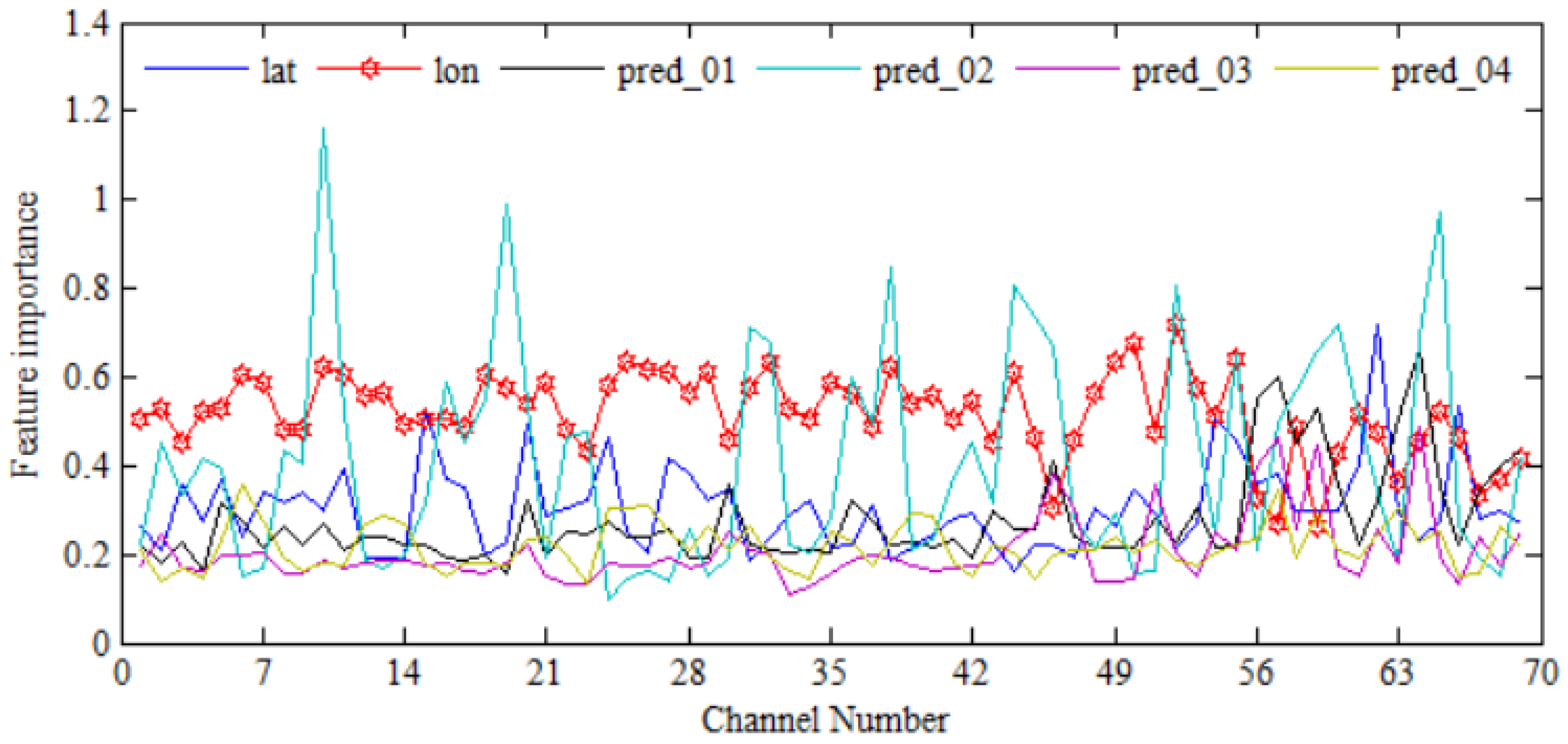
Furthermore, Figure 11 presents the feature importance of different feature variables to bias correction for the 69 selected channels. Here, “lon” represents the longitude of the field of view, “lat” represents the latitude, and other variable representations are similar to those in Figure 9.

As shown in Figure 11, overall, the longitude and latitude of the field of view contribute significantly and consistently to the brightness temperature of different FY-4A/GIIRS channels, a pattern that is attributed to the array bias in the FY-4A/GIIRS data [10,16]. This finding is of fundamental importance, indicating that for the vast majority of the selected mid-wave infrared channels, geographic coordinates are a core explanatory factor for their systematic biases. From an interpretability perspective, this confirms the physical validity of using geographic information as a fundamental forecast predictor and suggests that future bias correction models should place a strong emphasis on representing spatial information. The importance of “pred_02” (representing 200–50 hPa thickness) is greater in the correction process of certain channels. For example, the contribution of pred_02 for channel 1015 reaches 1.1569, and the peak of the weighting function for this channel is located in the troposphere. The significant differences in feature contribution rates between different channels in Figure 9 directly reflect the sensitivity of different detection channels to various atmospheric layers and parameters. The example of channel 1015 clearly demonstrates that, although geographic coordinates are generally important factors, for channels sensitive to specific atmospheric layers (such as the troposphere), the physical quantities describing the state of that layer (in this case, 200–50 hPa thickness, possibly related to temperature near the tropopause) become the most critical and even the most important basis for correction. This result provides micro-level evidence for the viewpoint that “channel selection is a prerequisite for intelligent correction,” indicating that the bias mechanisms for different channels vary and require differentiated modeling based on their sensitivities.

5. Discussion and Conclusions

This study establishes an integrated technical framework covering channel selection to intelligent bias correction. The channel selection of hyperspectral instruments is not an independent research topic separate from bias correction, but rather a necessary prerequisite to ensure the efficiency and targeted nature of the correction model [4,41,42]. The mid-wave infrared band of FY-4A/GIIRS contains a large number of channels with highly redundant information. If all channels were directly used in variational assimilation, it would not only impose a significant computational burden but also degrade assimilation performance due to noise introduced by many weakly sensitive channels. Therefore, this study adopts the entropy reduction method from the perspective of information theory and selects a subset of 69 channels that contribute significantly to the information gain of the analysis field. This step provides a solid data foundation for subsequent intelligent bias correction—channel selection addresses the question of “which channels should be corrected,” while bias correction based on ensemble learning focuses on “how to correct more accurately” using data-driven methods. These two components logically complement each other and jointly serve the ultimate goal of enhancing the direct assimilability of GIIRS observed brightness temperatures.

In the ensemble learning modeling, this study uses Random Forest, XGBoost, LightGBM, Decision Tree, and Extra Tree as base learners and constructs an ensemble model using a weighted averaging strategy. The experimental results show that, compared to single machine learning models and traditional offline linear methods, ensemble learning achieves better correction performance on the test dataset: its minimum RMSE (1.0140 K) outperforms all single models, and its maximum RMSE (1.4447 K) is better than the other four models, except for LightGBM, with the overall performance being the most balanced. This indicates that ensemble learning can effectively enhance the stability and generalization ability of the bias correction model by integrating the advantages of different models. However, the current ensemble framework only includes five base models, and there is still room for improvement in model diversity and representativeness. Incorporating a wider range of machine learning models in the future may further explore the potential of ensemble learning.

It is worth noting that, in the preprocessing phase of Section 2, to fully preserve the nonlinear variation characteristics of the bias and avoid the loss of effective training samples due to hard threshold truncation, this study did not set explicit removal thresholds for the difference between observed and simulated brightness temperatures (O-B). This means that some extreme O-B outliers (such as 5.98 K and −5.51 K for channel 1093, and 5.95 K and −6.00 K for channel 1094) were included in the training samples. The experimental results show that, due to its multi-model weighted average strategy, the ensemble learning model demonstrated good robustness against these extreme values, without significant overfitting or degradation in generalization ability. On one hand, this validates the advantage of the ensemble method in handling nonlinear bias features; on the other hand, it suggests that, when the training samples are sufficient and the model capacity is appropriate, retaining extreme outliers may help the model more broadly capture the complete distribution of the bias, rather than simply treating them as noise to be removed. Of course, the potential impact of extreme outliers still needs to be carefully evaluated in the context of specific weather scenarios (such as near the eye of a typhoon or convective cloud systems), which remains an area for further research.

The selection of forecast predictors directly impacts the physical plausibility and correction performance of bias correction. In this study, six forecast predictors were selected: longitude, latitude, 1000–300 hPa thickness, 200–50 hPa thickness, surface temperature, and total precipitable water. SHAP interpretability analysis indicates that geographic coordinates (longitude and latitude) make the most significant contribution to bias correction, which may be related to the observational geometry of geostationary satellites [30], regional climate background, and the spatial heterogeneity of surface features. At the same time, the analysis reveals the significant contribution of atmospheric state factors, such as the 200–50 hPa thickness, to specific channels (e.g., channel 1015)—this channel’s weighting function peak is located in the lower troposphere, yet the most significant contribution to its correction comes from physical quantities describing the state from the upper troposphere to the lower stratosphere. This finding provides micro-evidence for the vertical sensitivity differences across different channels and supports the idea that “channel selection is a prerequisite for intelligent correction.” Furthermore, SHAP analysis also preliminarily reveals the nonlinear relationship between forecast predictors and correction amounts, as well as interactions between factors, offering valuable insights into understanding complex machine learning models. This helps link data-driven results with physical explanations, thereby enhancing the model’s credibility.

This study has some limitations that need to be addressed in future work: (I) Data limitations: The model’s training and validation are entirely dependent on high-frequency clear-sky observation data during Typhoon Lekima. The generalization ability for other weather systems, different seasons, and cloud conditions still needs to be verified. (II) Operational gap: The offline training mode uses static model parameters, which cannot be updated in real-time with the atmospheric state. (III) Computational efficiency: Ensemble learning increases computational complexity, requiring a trade-off between accuracy and efficiency. (IV) NWP impact assessment: The impact of the bias correction on numerical weather prediction skill has not been assessed.

Building on the recognition of the above limitations, future research will focus on three directions: expanding the multi-sample dataset to verify the model’s generalization ability; exploring online model update mechanisms to bridge the operational gap; and conducting assimilation sensitivity experiments based on the NWP model to quantitatively assess the actual improvements in key elements such as typhoon tracks and precipitation forecasts from bias-corrected brightness temperatures.

References

1. Rabier, F.; Fourrié, N.; Chafäi, D.; Prunet, P. Channel selection methods for Infrared Atmospheric Sounding Interferometer radiances. Q. J. R. Meteorol. Soc. 2002, 128, 1011–1027. [Google Scholar] [CrossRef] [Scilit]
2. Geer, A.J. Correlated observation error models for assimilating all-sky infrared radiances. Atmos. Meas. Tech. 2019, 12, 3629–3657. [Google Scholar] [CrossRef] [Scilit]
3. Dee, D.P. Bias and data assimilation. Q. J. R. Meteorol. Soc. 2005, 131, 3323–3343. [Google Scholar] [CrossRef] [Scilit]
4. Auligné, T.; McNally, A.P.; Dee, D.P. Adaptive bias correction for satellite data in a numerical weather prediction system. Q. J. R. Meteorol. Soc. 2007, 133, 631–642. [Google Scholar] [CrossRef] [Scilit]
5. Harris, B.A.; Kelly, G. A satellite radiance-bias correction scheme for data assimilation. Q. J. R. Meteorol. Soc. 2001, 127, 1453–1468. [Google Scholar] [CrossRef] [Scilit]
6. Dee, D.P.; Uppala, S. Variational bias correction of satellite radiance data in the ERA-Interim reanalysis. Q. J. R. Meteorol. Soc. 2009, 135, 1830–1841. [Google Scholar] [CrossRef] [Scilit]
7. Francis, D.J.; Fowler, A.M.; Lawless, A.S.; Eyre, J.; Migliorini, S. The effective use of anchor observations in variational bias correction in the presence of model bias. Q. J. R. Meteorol. Soc. 2023, 149, 1789–1809. [Google Scholar] [CrossRef] [Scilit]
8. Jin, J.B.; Lin, H.X.; Segers, A.; Xie, Y.; Heemink, A. Machine learning for observation bias correction with application to dust storm data assimilation. Atmos. Chem. Phys. 2019, 19, 10009–10026. [Google Scholar] [CrossRef] [Scilit]
9. Huang, P.Y.; Guo, Q.; Han, C.P.; Zhang, C.M.; Yang, T.H.; Huang, S. An improved method combining ANN and 1D-Var for the retrieval of atmospheric temperature profiles from FY-4A/GIIRS hyperspectral data. Remote Sens. 2021, 13, 481. [Google Scholar] [CrossRef] [Scilit]
10. Wang, G.; Chen, J.; Wang, Y. Bias correction of channel brightness temperature of FY-4A hyperspectral GIIRS based on machine learning. Meteorol. Environ. Res. 2022, 13, 26–30. [Google Scholar] [CrossRef]
11. Qi, J.F.; Liu, C.Y.; Chi, J.W.; Li, D.L.; Gao, L.; Yin, B.S. An ensemble-based machine learning model for estimation of subsurface thermal structure in the South China Sea. Remote Sens. 2022, 14, 3207. [Google Scholar] [CrossRef] [Scilit]
12. Natras, R.; Soja, B.; Schmidt, M. Ensemble machine learning of random forest, AdaBoost and XGBoost for vertical total electron content forecasting. Remote Sens. 2022, 14, 3547. [Google Scholar] [CrossRef] [Scilit]
13. Nourani, V.; Dehghan, M.; Baghanam, A.H.; Kantoush, S.A. Dual purpose of Shapley Additive Explanation (SHAP) in model explanation and feature selection for artificial intelligence-based digital twin of wastewater treatment plant. J. Water Process. Eng. 2025, 75, 107947. [Google Scholar] [CrossRef] [Scilit]
14. Yang, J.; Zhang, Z.Q.; Wei, C.Y.; Lu, F.; Guo, Q. Introducing the new generation of Chinese geostationary weather satellites, Fengyun-4. Bull. Amer. Meteor. Soc. 2017, 98, 1637–1658. [Google Scholar] [CrossRef] [Scilit]
15. Xie, Q.; Li, D.Q.; Yang, Y.; Zhao, Y.H.; Li, H.; Zhu, S.J.; Pan, X. Exploring the assimilation of all-sky FY-4A GIIRS radiances and its forecasts for binary typhoons. IEEE J. Sel. Top. Appl. Earth Obs. Remote Sens. 2025, 18, 5949–5959. [Google Scholar] [CrossRef] [Scilit]
16. Yin, R.Y.; Han, W.; Gao, Z.Q.; Di, D. The evaluation of FY4A’s Geostationary Interferometric Infrared Sounder (GIIRS) long-wave temperature sounding channels using the GRAPES global 4D-Var. Q. J. R. Meteorol. Soc. 2020, 146, 1459–1476. [Google Scholar] [CrossRef] [Scilit]
17. Zhu, Y.Q.; Derber, J.; Collard, A.; Dee, D.; Treadon, R.; Gayno, G.; Jung, J.A. Enhanced radiance bias correction in the National Centers for Environmental Prediction’s Gridpoint Statistical Interpolation data assimilation system. Q. J. R. Meteorol. Soc. 2014, 140, 1479–1492. [Google Scholar] [CrossRef] [Scilit]
18. Wang, G.; Ye, S.; Xu, B.; Zhi, X.; Liu, Q.; Liu, Y.; Pan, Y.; Fan, C.; Zhang, T.; Xie, F. Generalized variational retrieval of full field-of-view cloud fraction and precipitable water vapor from FY-4A/GIIRS observations. Remote Sens. 2025, 17, 3687. [Google Scholar] [CrossRef] [Scilit]
19. Breiman, L. Random forests. Mach. Learn. 2001, 45, 5–32. [Google Scholar] [CrossRef] [Scilit]
20. Wishnuwardana, R.J.; Omar, M.B.; Zabiri, H.B.; Faqih, M.; Bingi, K.; Ibrahim, R. Optuna-LightGBM: An Optuna hyperparameter optimization framework for the determination of solvent components in acid gas removal unit using LightGBM. Clean. Eng. Technol. 2025, 28, 101054. [Google Scholar] [CrossRef] [Scilit]
21. Shin, K.; Kim, K.; Song, J.J.; Lee, G.W. Classification of precipitation types based on machine learning using dual-polarization radar measurements and thermodynamic fields. Remote Sens. 2022, 14, 3820. [Google Scholar] [CrossRef] [Scilit]
22. Rehan, I.; Rehman, M.U.; Aamir, M.; Islam, S. A CatBoost and ExtraTrees-based softvoting ensemble approach for non-invasive diabetes detection using hair LIBS spectral data. Microchem. J. 2025, 217, 114980. [Google Scholar] [CrossRef] [Scilit]
23. Shahhosseini, M.; Hu, G.P.; Pham, H. Optimizing ensemble weights and hyperparameters of machine learning models for regression problems. Mach. Learn. Appl. 2022, 7, 100251. [Google Scholar] [CrossRef] [Scilit]
24. Wang, G.; Han, W.; Yuan, S.; Wang, J.; Yin, R.Y.; Ye, S.; Xie, F. Retrieval of high-frequency temperature profiles by FY-4A/GIIRS based on generalized ensemble learning. J. Meteorol. Soc. Jpn. 2024, 102, 241–264. [Google Scholar] [CrossRef] [Scilit]
25. Saunders, R.; Hocking, J.; Turner, E.; Rayer, P.; Rundle, D.; Brunel, P.; Vidot, J.; Roquet, P.; Matricardi, M.; Geer, A.; et al. An update on the RTTOV fast radiative transfer model (currently at version 12). Geosci. Model Dev. 2018, 11, 2717–2737. [Google Scholar] [CrossRef] [Scilit]
26. Wang, W.; Huang, P.Y.; Xu, N.; Li, J.; Di, D.; Zhang, Z.Q.; Gao, L.; Ji, Z.M.; Min, M. Evaluating the first year on-orbit radiometric calibration performance of GIIRS onboard Fengyun-4B. IEEE Geosci. Remote Sens. Lett. 2024, 21, 002905. [Google Scholar] [CrossRef] [Scilit]
27. Ma, Z.; Li, J.; Han, W.; Li, Z.L.; Zeng, Q.C.; Menzel, W.P.; Schmit, T.J.; Di, D.; Liu, C.-Y. Four-dimensional wind fields from geostationary hyperspectral infrared sounder radiance measurements with high temporal resolution. Geophys. Res. Lett. 2021, 48, e2021GL093794. [Google Scholar] [CrossRef] [Scilit]
28. Min, M.; Wu, C.Q.; Li, C.; Liu, H.; Xu, N.; Wu, X.; Chen, L.; Wang, F.; Sun, F.L.; Qin, D.Y. Developing the science product algorithm testbed for Chinese next-generation geostationary meteorological satellites: Fengyun-4 series. J. Meteorol. Res. 2017, 31, 708–719. [Google Scholar] [CrossRef] [Scilit]
29. Zhang, Q.; Yu, Y.; Zhang, W.M.; Luo, T.L.; Wang, X. Cloud detection from FY-4A’s geostationary interferometric infrared sounder using machine learning approaches. Remote Sens. 2019, 11, 3035. [Google Scholar] [CrossRef] [Scilit]
30. Di, D.; Li, J.; Han, W.; Bai, W.G.; Wu, C.Q.; Menzel, W.P. Enhancing the fast radiative transfer model for FengYun-4 GIIRS by using local training profiles. J. Geophys. Res-Atmos. 2018, 123, 12583–12596. [Google Scholar] [CrossRef] [Scilit]
31. Matricardi, M. A principal component based version of the RTTOV fast radiative transfer model. Q. J. R. Meteorol. Soc. 2010, 136, 1823–1835. [Google Scholar] [CrossRef] [Scilit]
32. Zhu, L.Y.; Zhou, R.L.; Di, D.; Bai, W.G.; Liu, Z.J. Retrieval of atmospheric water vapor content from AHI/H8 using both physical and random forest methods—A case study for Typhoon Maria (201808). Remote Sens. 2023, 15, 498. [Google Scholar] [CrossRef] [Scilit]
33. Cai, X.; Bao, Y.S.; Petropoulos, G.P.; Lu, F.; Lu, Q.F.; Zhu, L.H.; Wu, Y. Temperature and humidity profile retrieval from FY4-GIIRS hyperspectral data using artificial neural networks. Remote Sens. 2020, 12, 1872. [Google Scholar] [CrossRef] [Scilit]
34. Malmgren-Hansen, D.; Laparra, V.; Nielsen, A.A.; Camps-Valls, G. Statistical retrieval of atmospheric profiles with deep convolutional neural networks. ISPRS J. Photogramm. Remote Sens. 2019, 158, 231–240. [Google Scholar] [CrossRef] [Scilit]
35. Otkin, J.A.; Potthast, R.; Lawless, A.S. Nonlinear bias correction for satellite data assimilation using Taylor series polynomials. Mon. Weather Rev. 2018, 46, 263–285. [Google Scholar] [CrossRef] [Scilit]
36. Zhang, X.W.; Xu, D.M.; Min, J.Z.; Li, H.; Shen, F.F.; Lei, Y.H. A machine learning-based bias correction scheme for the all-sky assimilation of AGRI infrared radiances in a regional OSSE framework. IEEE Trans. Geosci. Remote Sens. 2024, 62, 5407314. [Google Scholar] [CrossRef] [Scilit]
37. Cui, T.Y.; Wu, D.J.; Wang, Z.J. Catboost-SHapley Additive exPlanations (SHAP) car following model: Explaining model features in mixed traffic conditions. Multimodal Transp. 2026, 5, 100284. [Google Scholar] [CrossRef] [Scilit]
38. Noh, Y.-C.; Sohn, B.-J.; Kim, Y.; Joo, S.; Bell, W.; Saunders, R. A new infrared atmospheric sounding interferometer channel selection and assessment of its impact on Met Office NWP forecasts. Adv. Atmos. Sci. 2017, 34, 1265–1281. [Google Scholar] [CrossRef] [Scilit]
39. Vittorioso, F.; Guidard, V.; Fourrié, N. An infrared atmospheric sounding interferometer-new generation (IASI-NG) channel selection for numerical weather prediction. Q. J. R. Meteorol. Soc. 2021, 147, 3297–3317. [Google Scholar] [CrossRef] [Scilit]
40. Lim, A.H.N.; Li, Z.L.; Nebuda, S.E.; Jung, J.A. Assimilation of radiance tendency observations from geostationary satellites in NCEP’s global forecast system. Q. J. R. Meteorol. Soc. 2025, 151, e70005. [Google Scholar] [CrossRef] [Scilit]
41. Collard, A.D. Selection of IASI channels for use in numerical weather prediction. Q. J. R. Meteorol. Soc. 2007, 133, 1977–1991. [Google Scholar] [CrossRef] [Scilit]
42. Li, Z.L.; Lim, A.H.N.; Jung, J.A.; Schmit, T.J.; Li, J.; Menzel, W.P.; Moeller, S.-C.; Ma, Y.T. Exploration of the use of short-wave infrared radiances in weather forecasts: Part I. Methodologies for bias correction and quality control. Q. J. R. Meteorol. Soc. 2025, 151, e5020. [Google Scholar] [CrossRef] [Scilit]
Figure 1. Histogram of O-B before brightness temperature bias correction for FY-4A/GIIRS channels: (a) Channel 1093, (b) Channel 1094. The statistical period is from 8 to 10 August 2019 (UTC) during the high-frequency observation period of Typhoon Lekima, with 11,483 clear-sky field of view samples.
Remotesensing 18 00748 g001
Figure 2. Study region: (a) AGRI cloud mask (CLM) product and (b) cloud fraction distribution over the GIIRS high-frequency observation region.
Remotesensing 18 00748 g002
Figure 3. Channel selection: (a) Optimal GIIRS mid-wave channel combination based on the entropy reduction method, with colored vertical lines indicating the central wavenumber positions of the selected channels; (b) The distribution of weighting functions. Colors range from blue to red, representing increasing channel numbers. Channels 1093, 1094, and 1015 are shown in bold. The inset provides an enlarged view of the weighting function peaks for these three channels.
Remotesensing 18 00748 g003
Figure 4. Flowchart of the proposed bias correction method for FY-4A/GIIRS mid-wave infrared channel brightness temperatures.
Remotesensing 18 00748 g004
Figure 5. Scatter plot distributions of bias correction results for different models: (a) Random Forest—Training dataset; (b) Random Forest—Test dataset; (c) XGBoost—Training dataset; (d) XGBoost—Test dataset; (e) LightGBM—Training dataset; (f) LightGBM—Test dataset; (g) Decision Tree—Training dataset; (h) Decision Tree—Test dataset; (i) Extra Tree—Training dataset; (j) Extra Tree—Test dataset; (k) Ensemble Learning—Training dataset; (l) Ensemble Learning—Test dataset.
Remotesensing 18 00748 g005aRemotesensing 18 00748 g005b
Figure 6. Probability density function (PDF) distributions of channel brightness temperature biases before and after correction: (a) Channel 1093, Training dataset; (b) Channel 1093, Test dataset; (c) Channel 1094, Training dataset; (d) Channel 1094, Test dataset.
Remotesensing 18 00748 g006
Figure 7. Weight distribution of each base model in the ensemble learning model. Blue line: Random Forest; dark green line: XGBoost, red line: LightGBM; light green line: Decision Tree; magenta line: Extra Tree.
Remotesensing 18 00748 g007
Figure 8. Distribution of RMSE between the corrected brightness temperatures and the simulated brightness temperatures for the selected channels after correction by different models: (a) training dataset; (b) test dataset.
Remotesensing 18 00748 g008
Figure 9. Analysis of brightness temperature correction results based on the SHAP interpreter: (a) feature density scatter distribution with colors representing feature values (red: low values, blue: high values); (b) feature importance distribution; (c) heatmap of model results.
Remotesensing 18 00748 g009
Figure 10. Interaction relationships between different feature variables: (a) forecast predictor 2 and 4; (b) forecast predictor 3 and 4; (c) longitude of the field of view and forecast predictor 1; (d) longitude of the field of view and forecast predictor 4.
Remotesensing 18 00748 g010
Figure 11. Distribution of the feature importance of different feature variables to the selected channels.
Remotesensing 18 00748 g011