Exploring the Capabilities of CuSum-Near-Real-Time Analysis Using Sentinel-1 Data for Field Monitoring: How Can a Change Detection Method Complement Information from Earth Observations?

Highlights

What are the main findings?

• The cumulative sum near-real-time detection method applied on Sentinel-1 provides additional information to the polarisation backscatter.
• The yearly mean number of changes obtained using cumulative sum near-real-time analysis on Sentinel-1 varies according to the category of crops.

What are the implications of the main findings?

• The monthly averaged number of changes can be used as additional data for phenology or soil monitoring.
• Cumulative sum may be used for crop classification and biomass monitoring in temperate cultivated fields.

Abstract

This study analyses the potential of a change detection method—the near-real-time cumulative sum change point detection method (CuSum-NRT)—applied to Sentinel-1 C-band synthetic aperture radar (SAR) data to monitor crops and identify field work based on a monthly number of changes. The temporal evolution of the number of changes occurring on Sentinel-1 backscatter at both VV and VH polarisations averaged at field scale was analysed over five years (2017–2021) and compared with NDVI derived from the Sentinel-2 multispectral instrument (MSI) sensor over more than 1000 fields in the southwest of France. The monthly number of changes detected did not show a significant difference between months with soil work and months with no soil work, so further analysis on the dates of changes should be conducted. The number of changes based on VV was found to poorly correlate with the VV backscatter (R_global = 0.25), and that based on VH was found to moderately correlate with the VH backscatter (R_global = 0.61): CuSum provides additional information compared to backscatter alone. The results also showed that the number of changes detected using CuSum-NRT is correlated to NDVI, mostly positively for the VH polarisation (R_max = 0.73, p-value < 0.05) and negatively for the VV polarisation (R_min = −0.69, p-value < 0.005). Furthermore, the analysis of crop groups (cereals, oilseeds, protein crops, fodder, vegetables, others) displayed statistically significant differences in terms of the annual number of changes occurring on both VH and VV polarisations, which has potential applications in crop classification.

1. Introduction

Spatial and temporal information about agricultural practices is important in order to maintain a sustainable development in terms of environment, economy, and agronomy [1,2]. Earth observation (EO) data are now widely used for the different vegetation types and states in the agricultural practices at a large scale [3,4]. Multispectral and synthetic aperture radar (SAR) sensors are commonly considered for crop monitoring as they provide information on land use [5,6,7,8], crop spectral absorbance, soil roughness, soil moisture, and vegetation [9,10,11]. Data obtained using these sensors also provide information on crop parameters such as biomass, grain yields, or phenological cycles [12,13,14,15,16,17,18,19].

In recent years, a wide range of algorithms have been employed to monitor agricultural fields using microwave EO data, particularly Sentinel-1 imagery, as they can provide information under cloudy conditions. These methods aim to detect changes in crop phenology [20,21,22,23,24,25,26], to classify crop types [27,28], and to detect agricultural practices [29,30]. Time series analysis approaches, such as harmonic fitting (breaks for additive season and trend, BFAST [31,32,33]) and moving averages (MOSUM, [34]) have been used to extract trends and seasonal patterns. Machine learning methods such as random forests, support vector machines (SVM), and neural networks were employed to classify crop types and detect abrupt changes based on temporal and spectral features [26,29,30]. Several change detection methods: BFAST, continuous change detection, change vector analysis (CVA), and cumulative sum (CuSum) methods exhibited a strong potential in identifying anomalies or structural changes in the radar backscatter signal for the monitoring of forest cover change [33,35,36,37,38,39,40,41,42,43]. However, many of these algorithms require dense and regularly sampled time series or are sensitive to the speckle noise affecting SAR images. Among these approaches, CuSum has been applied to monitor forest disturbances, including degradation and deforestation, and to characterize land use dynamics, including differentiating forest from other types of land use land cover (LULC) based on the temporal frequency of detected changes [44,45,46,47]. Recently, the near-real-time implementation of CuSum has shown that non-forest areas, including agricultural areas, systematically exhibit higher annual change frequencies than forested areas [47,48].

These previous observations suggest that the temporal accumulation of CuSum-NRT detections may capture information related not only to land cover transitions but also to vegetation dynamics and management practices. Building on this methodological framework, the present study investigates whether the monthly accumulated number of changes detected by CuSum-NRT over agricultural parcels is related to crop type, radar polarisation, and spectral vegetation indicators such as NDVI. The objective is, therefore, to assess the potential of CuSum-NRT applied to Sentinel-1 data as a complementary information source for agricultural monitoring, rather than to perform a comparative evaluation of change detection algorithms.

To test this approach, more than one thousand fields were selected in the southwest of France over the 2017–2021 period. The analysis was performed on the crops (sunflower, maize, rapeseed, winter soft wheat) cultivated at the Auradé and Lamasquère stations of the Integrated Carbon Observation System (ICOS) network during the study period. Then, a broader analysis was achieved on the 61 crop types cultivated in the whole study area. The correlations between the monthly number of changes, their polarisation mean backscatter, and NDVI were studied for each crop type. The yearly number of changes for each group of crops and crop types was also analysed.

The article is composed of two main sections, organized as follows: Section 2 presents the area, the available data, and the CuSum methodology. Section 3 presents the analysis of the results. Section 3.1 presents the field-scale results in Auradé and Lamasquère, then Section 3.2 presents the results for each crop type grown in these two fields, which are generalized over the entire study area. Section 3.3 presents the generalisation of the results on all crop types available over the area and the correlation results between the monthly mean number of detections and the monthly mean NDVI.

2. Study Area, Data, and Methods

2.1. Study Area

This area has been monitored since 2007 in the context of the Regional Spatial Observatory Southwest (OSR SO, https://osr.cesbio.cnrs.fr/, accessed on 11 December 2025). This observatory is part of the Pyrenees Garonne Regional Workshop Area (ZA PYGAR [49]), the OZCAR research infrastructure in the critical zone [50], and has two flux sites (located near the villages of Auradé and Lamasquère, FR-Aur and FR-Lam) belonging to the Integrated Carbon Observation System (ICOS, [51]).

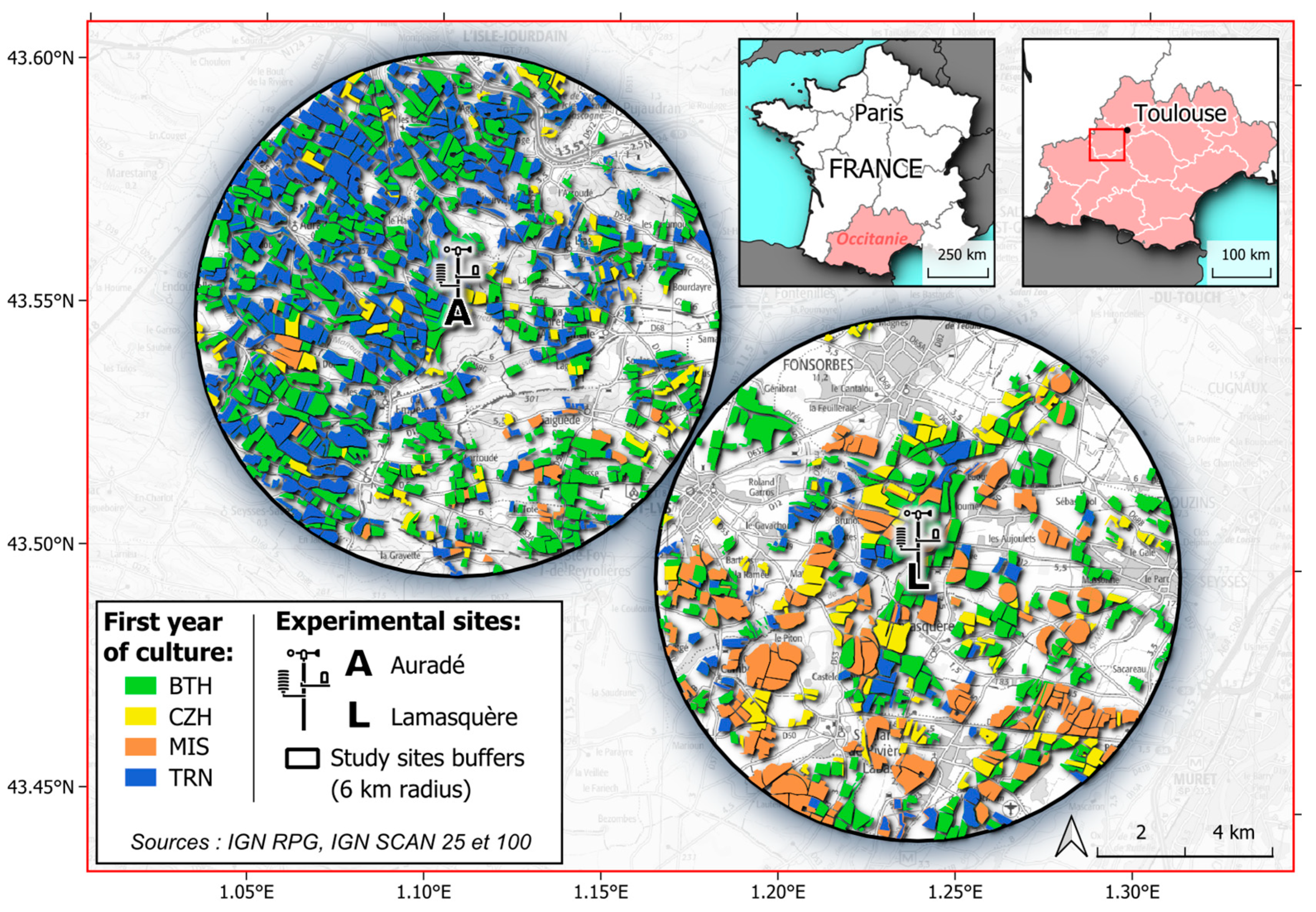
The study area is located in southwestern France (Occitanie region, 43.52°N, 1.17°E) and covers two 6 km radius circles centered on the experimental fields of Lamasquère (irrigated) and Auradé (rainfed) (Figure 1). They are equipped with meteorological sensors that provide climatic data used to interpret satellite observations and CuSum-NRT results. The landscape is mainly agricultural, with grasslands and annual crops dominating, while urban areas, forests, and water bodies cover about 10% of the surface. Land use data are derived from the French Graphical Land Plot Register (RPG) provided by the Services and Payment Agency. The crops cultivated in Auradé and Lamasquère were analysed in the 6 km radius circles: winter rapeseed, soft winter wheat, sunflower, and corn. Soft wheat and sunflower are the most common (15–25%), followed by corn (≈10%). Corn and soybeans are the only irrigated crops. Field sizes range from 2 to 80 ha, with half under 5 ha and only 15% over 10 ha. Median parcel sizes are the smallest for rapeseed and barley (~4.4 ha) and the largest for irrigated crops (corn ≈ 5.9 ha, soybeans ≈ 6.4 ha). The region is controlled by a temperate climate with annual rainfall between 592 mm (2021) and 827 mm (2018), showing a clear seasonal pattern, wet in spring and autumn, dry in summer. Mean summer temperatures reach 20–25 °C, dropping to 0–5 °C in winter. The relief of the area alternates between valleys, terraces, and clay-limestone hills, with variable soil fertility and hydromorphic constraints. Two main cropping systems coexist: irrigated (corn) and rainfed (wheat, rapeseed, sunflower). Soils are split into four USDA texture classes: silty loam (≈34%), clay loam (≈28%), silty clay loam (≈24%), and loam (≈14%), textures that retain water well but are prone to compaction when silt content is high.

Overall, the study site combines diverse soils, topography, and cropping systems representative of southwestern France’s agricultural landscapes, making it well-suited for Sentinel-1–based crop monitoring and validation of the CuSum-NRT method.

2.2. Data

2.2.1. Sentinel-1 Data

Sentinel-1 is a mission developed by the European Space Agency (ESA) as part of the Copernicus program. It consists of a constellation of two satellites, launched in 2014 and 2016, which remained operational throughout our monitoring period (2017–2021). These satellites, Sentinel-1A and Sentinel-1B, are equipped with a synthetic aperture radar (SAR) sensor operating in the C-band (C-SAR) at a frequency of 5.405 GHz. They acquire images in co- and cross-polarisation modes (VV and VH) with a ground resolution of 20 × 22 m, corresponding to a pixel resolution of 9.54 m after the preprocessing steps applied by VisioTerra [52].

A total of 315 ascending images were processed for the 2016–2021 period (

Table 1. Number of Sentinel-1 ascending images downloaded per year over the 2016–2022 period.

Year	2016	2017	2018	2019	2020	2021	2022
Number of Sentinel-1 images	11	60	60	58	61	62	3

). Preprocessing steps included orbit correction, thermal noise reduction [53], terrain correction [54], and speckle removal using a bilateral filter [55]. The speckle removal was performed using a pixel window of size 3.

2.2.2. Sentinel-2 Data

Sentinel-2 is also a mission developed by the European Space Agency (ESA) for the Copernicus program. It is composed of two satellites (Sentinel-2A and Sentinel-2B) launched in 2015 and 2016, respectively. They carry onboard the multispectral instrument (MSI) sensor with 13 operational wavelengths (from 443 nm to 2190 nm) and a 20.6-degree field of view [56]. The surface reflectance (SR) at 10 m pixel resolution from Level 2A was used. Only images with a cloud cover lower than 30% were selected, resulting in 142 available images. These images were used to derive the Normalized Vegetation Index (NDVI) over the study area from 2017 to 2021.

Both Sentinel-1 and Sentinel-2 images were obtained from VtWeb (https://visioterra.org/VtWeb/, accessed on 6 August 2023).

2.2.3. In Situ Measurement Sites

Lamasquère and Auradé are two sites with near-real-time monitoring of precipitation, as well as other meteorological and biophysical parameters. The agricultural practices of Auradé and Lamasquère (accessible via the OSR SO environmental information system, https://osr.cesbio.cnrs.fr/, accessed on 11 December 2025), including plowing, stubble cultivation, sowing, harvesting, and other soil management operations, were collected from farmers and used in this study to analyse satellite signals and parameters derived from CuSum. Different crop types were harvested during the 2017–2021 period, as shown in

Table 2. Cultures in the ICOS plots of Lamasquère and Auradé from 2017 to 2021.

Plot	2017	2018	2019	2020	2021
Lamasquère	Corn	Winter soft wheat	Corn	Winter soft wheat	Fava bean, corn
Auradé	Winter soft wheat	Winter rapeseed	Winter soft wheat	Fava bean, sunflower	Spring durum wheat

. The precipitation values are available in Figure S1.

2.3. CuSum Near-Real-Time (NRT) Method

The cumulative sum (CuSum) is based on the sum of the difference between the time series and its mean. The date corresponding to the maximum sum of the residuals is considered to be the date of change, when the mean of the time series is crossed [42,48,57]. To confirm the validity of the detected change, a bootstrap analysis was applied with 500 iterations. This analysis removes the potential effect of the temporal dimension by performing a random permutation on the original time series. The amplitude of the residuals of the shuffled time series is then analysed, and if it is lower than the original amplitude of the residuals, the iteration is considered ‘valid’. This step is performed 500 times and allows for computing a confidence level of the change (CL) above which a critical threshold (Tc) is set to consider a change valid. Tc is the input sensitivity parameter. For the rest of the study, a change will be considered as the detection of the shift in Sentinel-1 time series as defined in the CuSum methodology.

In this study, the CuSum NRT was applied to the time series of Sentinel-1 C-band backscatter (γ0) at VV and VH polarisations. CuSum NRT is the application of CuSum cross in a sliding window composed of 14 images over a time period, with a window step size of one. It allows the detection of a change with minimal delay (up to 3 images are necessary after a change occurred to accurately date the change). Following the method applied over forests and discussed in [48], we selected a sliding window consisting of 14 images (11 ‘before’ and 3 ‘after’) and a Tc of 92%, as it resulted in numerous changes detected on non-forest vegetation area (including agricultural areas). In order to ensure a proper analysis of the whole time series, 11 images before 1 January 2016 and 3 images after 31 December 2021 were considered, but only changes detected with dates between 1 January 2016 and 31 December 2021 were kept. The delay of detection does not depend on time but on the number of images due to the statistical properties of the methodology.

In the following, the pixel-wise changes detected using the CuSum are cumulated on a monthly basis and averaged at the field scale using the information contained in the RPG database. Multiple detections of the same date are considered to be only one change.

2.4. Statistics

The correlations between NDVI, VV, and VH backscatter with the VV-based and the VH-based number of changes were analysed. An ordinary least squares (OLS) regression was performed using the Python (3.13) scikit package with a Pearson test. The inter-group difference size effects were analysed using a bootstrap based on a block approach at the parcel level (500 iterations). The results were considered significant at p-value < 0.05, very significant at p-value < 0.005, and highly significant at p-value < 0.0005.

3. Results

3.1. Analysis of Behaviors Observed at Experimental Plots

3.1.1. Vegetation Indexes and Backscatter Data

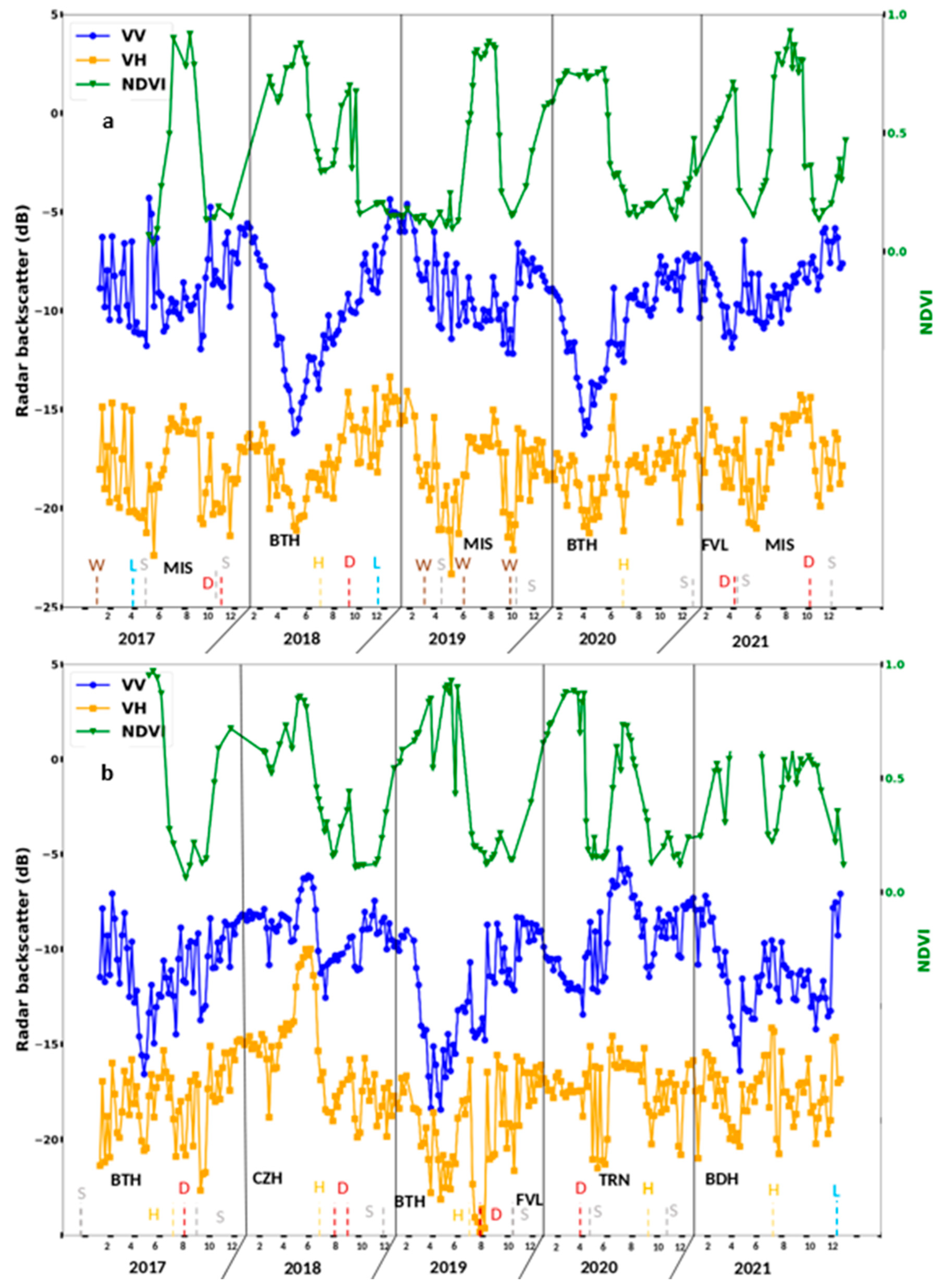
The NDVI indices were computed from Sentinel-2 and the VV and VH backscatter from Sentinel-1 over January 2017–December 2021 on both Lamasquère (Figure 2a) and Auradé (Figure 2b) sites. In Lamasquère (Figure 2a), the VV and VH backscatter showed different patterns according to the crop type. After sowing corn in May 2017, the VH backscatter increased conjointly with the NDVI, respectively, from −21 dB to −15 dB and from 0.1 to 0.9, until stabilising in July to August. Both then decreased in August to −21 dB and to 0.2, contrary to the VV backscatter that showed a short peak increase from −12 dB to −5 dB. This pattern also happened after the sowing of maize in both 2019 and 2021. After the sowing of winter soft wheat in October 2017, both VV and VH backscatter increased to −7 dB and −16 dB, respectively, until January. In January, the signal decreased significantly until May (a difference of 10 dB for VV, 7 dB for VH). The NDVI signal increased from 0.2 in December 2017 to 0.9 in May 2018; then it decreased sharply to 0.3. The same pattern also occurred in 2020 after the sowing of winter soft wheat.

From May 2018 to February 2019, both VV and VH backscatter increased steadily from −16.4 dB and −21.5 dB to −7 dB and −16 dB, respectively. A stubble cultivation event in September resulted in a peak increase in the VH backscatter from −20 dB to −14.9 dB and a peak decrease in NDVI, from 0.7 to 0.36.

Similarly to Lamasquère, in Auradé (Figure 2b), the sowing of winter soft wheat resulted in a short period of increasing VV and VH backscatter (~2 months) and, then, a decrease of ~9 dB for VV and ~5 dB for VH, while the NDVI continued to increase.

The sowing of winter rapeseed in Auradé resulted in a steady increase in VV and VH backscatter for 7 months (to reach a difference with the backscatter of 5 dB before sowing). The signal then increased rapidly over a month (+3 dB for VV and +5 dB for VH) before decreasing due to the harvest. The pattern of both polarisations is similar to NDVI.

The sowing of sunflower resulted in a decrease in the VH backscatter for a month (−4 dB) and an increase in the VV backscatter (+2 dB). Then, backscatter at both polarisations increased over a month (+3 dB for VV, +6 dB for VH), similarly to NDVI. Then, NDVI and VV decreased until the day of harvest, but VH showed a stable backscatter and decreased only on the date of harvest.

3.1.2. CuSum-Based Number of Changes

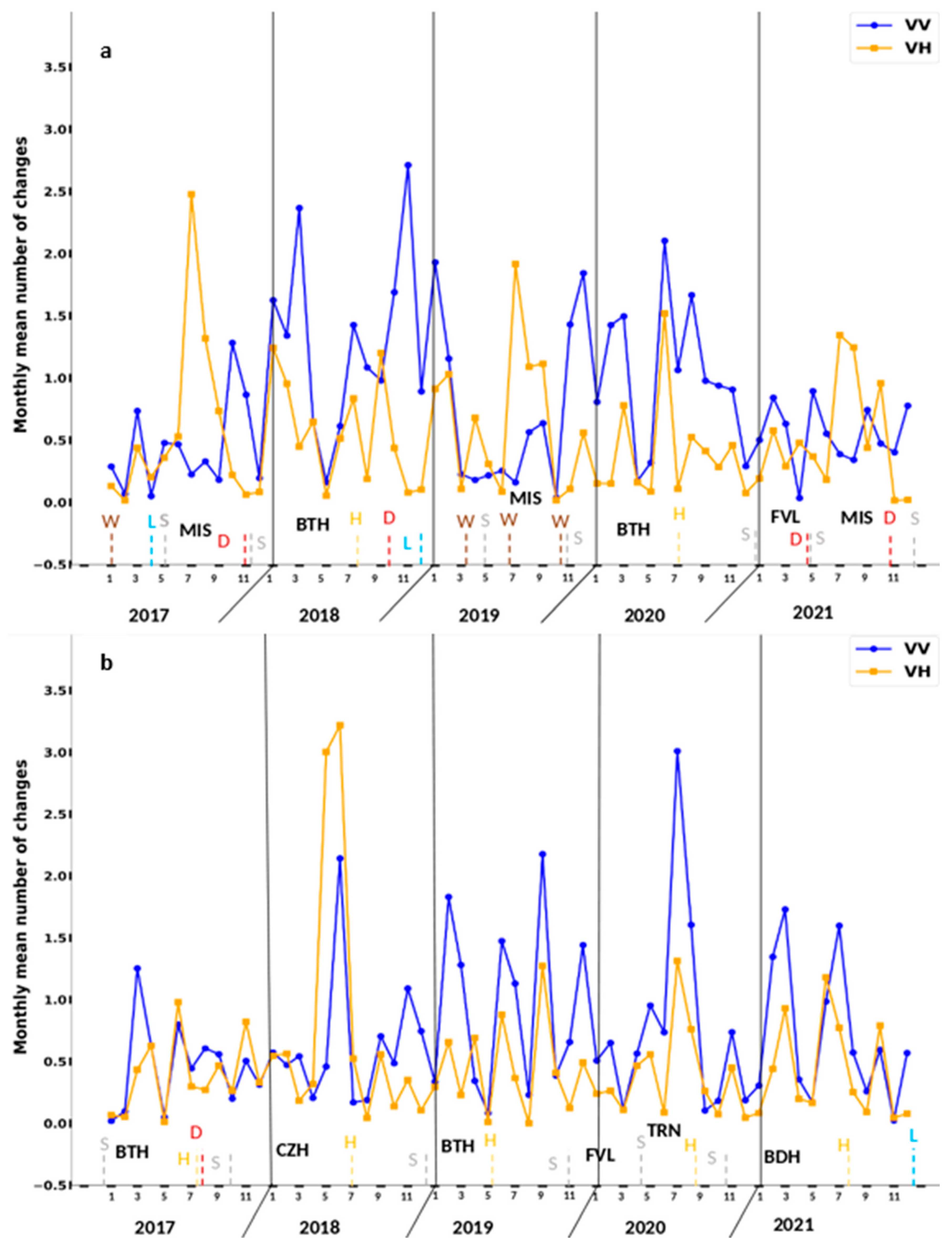
Time series of the monthly mean number of changes for Lamasquère and Auradé (Figure 3a and Figure 3b, respectively) showed that, in comparison with the different vegetation indices, a higher number of changes (>2) was observed for VH during the growth phase of maize and rapeseed than for VV. In August 2018 in Lamasquère, the number of changes increased similarly to the vegetation indices during a short period following the harvest of BTH. A similar pattern was observed with a lower amplitude in Auradé following the winter soft wheat sowing in 2017 and 2019.

The number of changes based on VV was higher during the growth phase of winter soft wheat, winter hard wheat, sunflower, and fava bean. A high number of changes in VV was also observed during time periods with a very low NDVI (<0.2), such as November/December 2018, on both sites.

3.2. Analysing the Main Crops over All Fields Within the Study Area

3.2.1. Monthly Number of Changes and NDVI from the Two Main Winter Crops (Winter Soft Wheat, Winter Rapeseed)

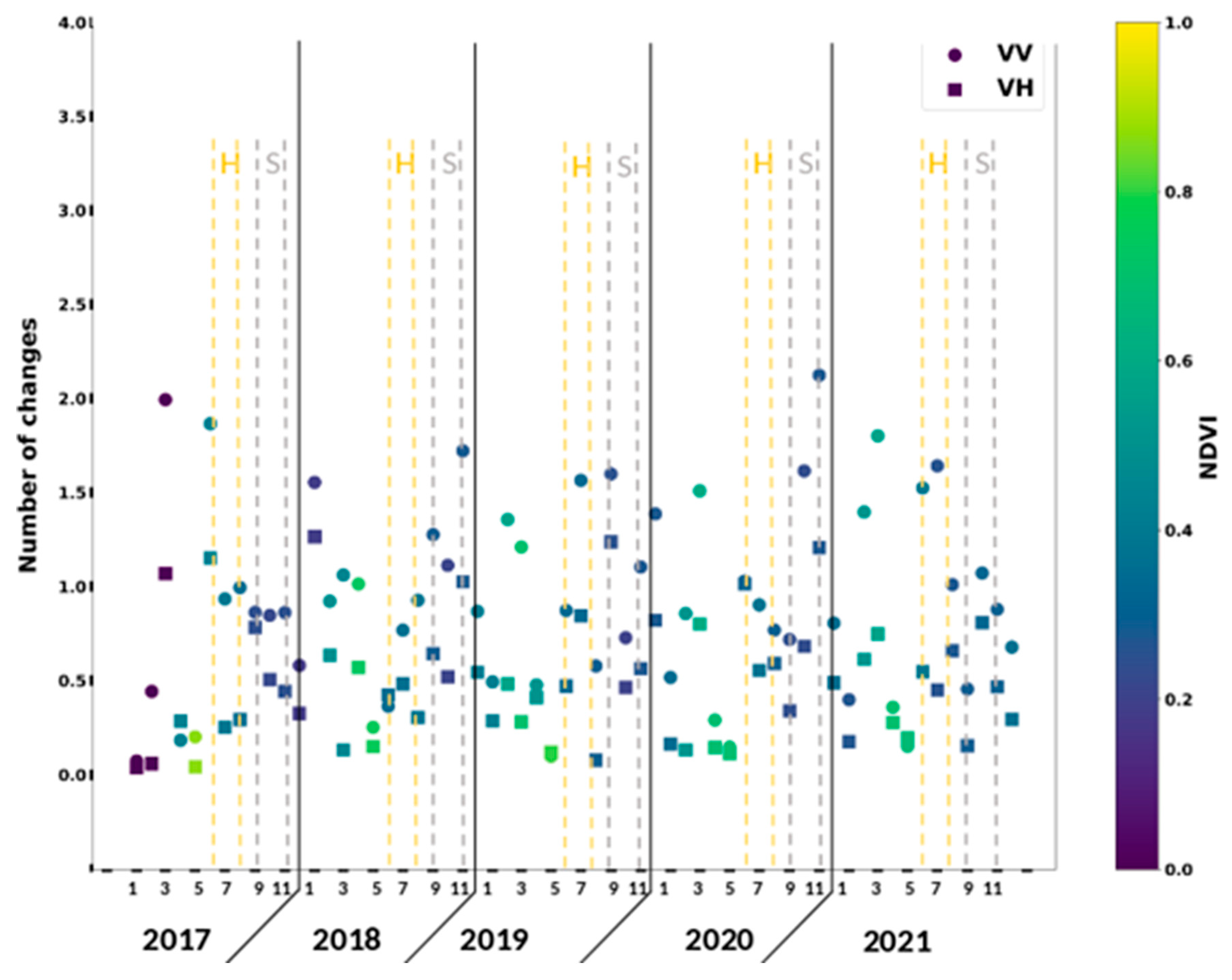
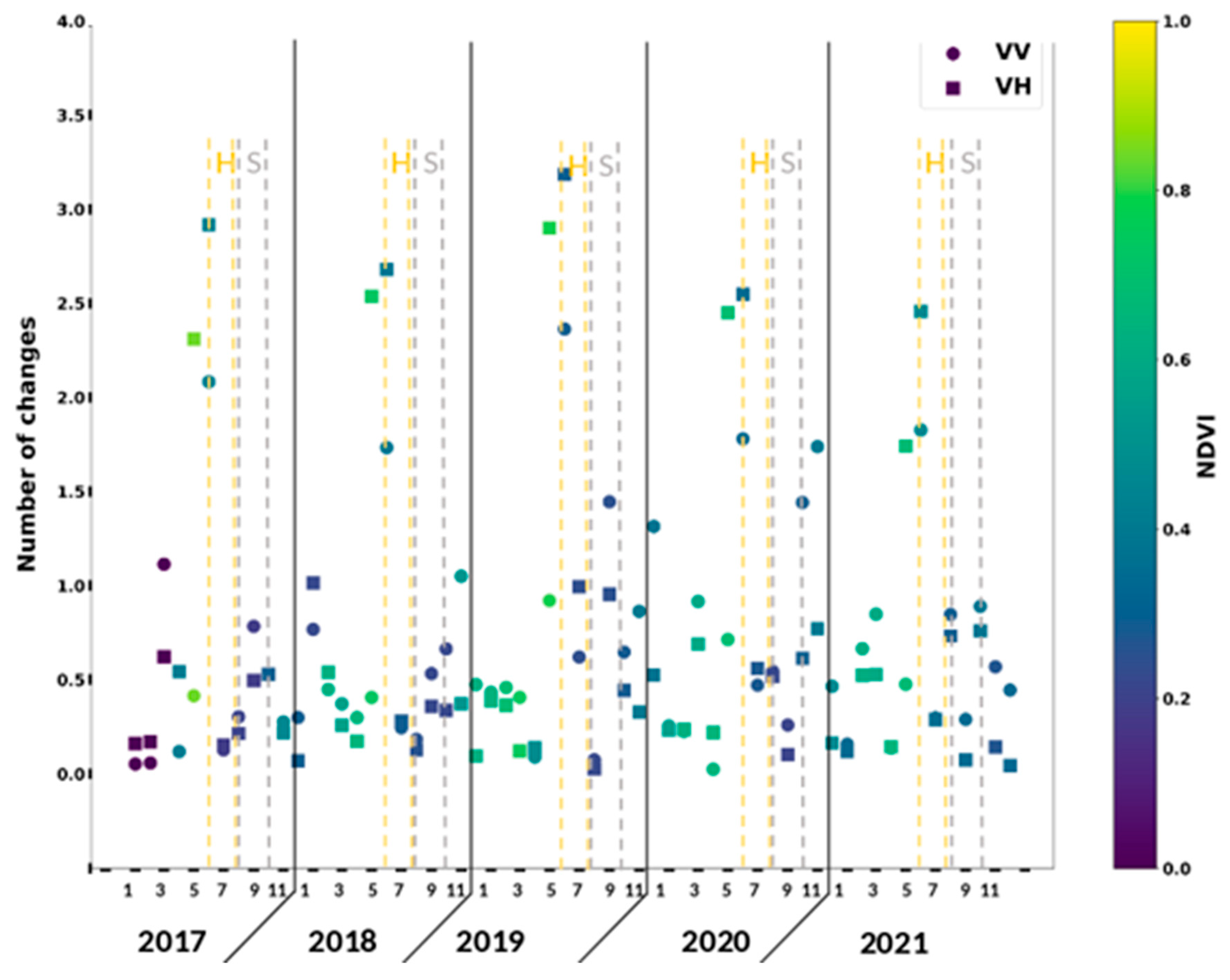
Figure 4 presents the monthly mean number of changes of the winter soft wheat averaged over all the cultivated fields of the study area from 2017 to 2021 using both VV and VH polarisations. The colors represent the monthly NDVI values. The NDVI values increase from less than 0.4 in January to more than 0.8 in May for all years, except 2017. The number of changes based on VV increases from January to March (~1.6–~1.8), in line with the vegetation growth, before decreasing sharply in April and May to ~0.3. It then increases starting in June, at the beginning of the harvest period, until November/December, after the sowing period, reaching 1.5~2. The number of changes based on VH shows a similar pattern to VV, with fewer changes overall. Despite significant inter-annual changes in precipitation in the Midi-Pyrenees region (e.g., summer 2020 was characterised by a deficit in rainfall up to 80% from the Meteo-France reference period, 1981–2010 average, causing a drought [58] and delayed sowing (e.g., late sowing in winter 2020)), all years exhibited a similar range of changes. In this region, refs. [8,15] showed that the γ⁰_VV backscatter coefficient of winter wheat increases during the winter and fluctuates with precipitation, then decreases from the end of February when vegetation starts to grow. The number of changes fluctuates following the same pattern.

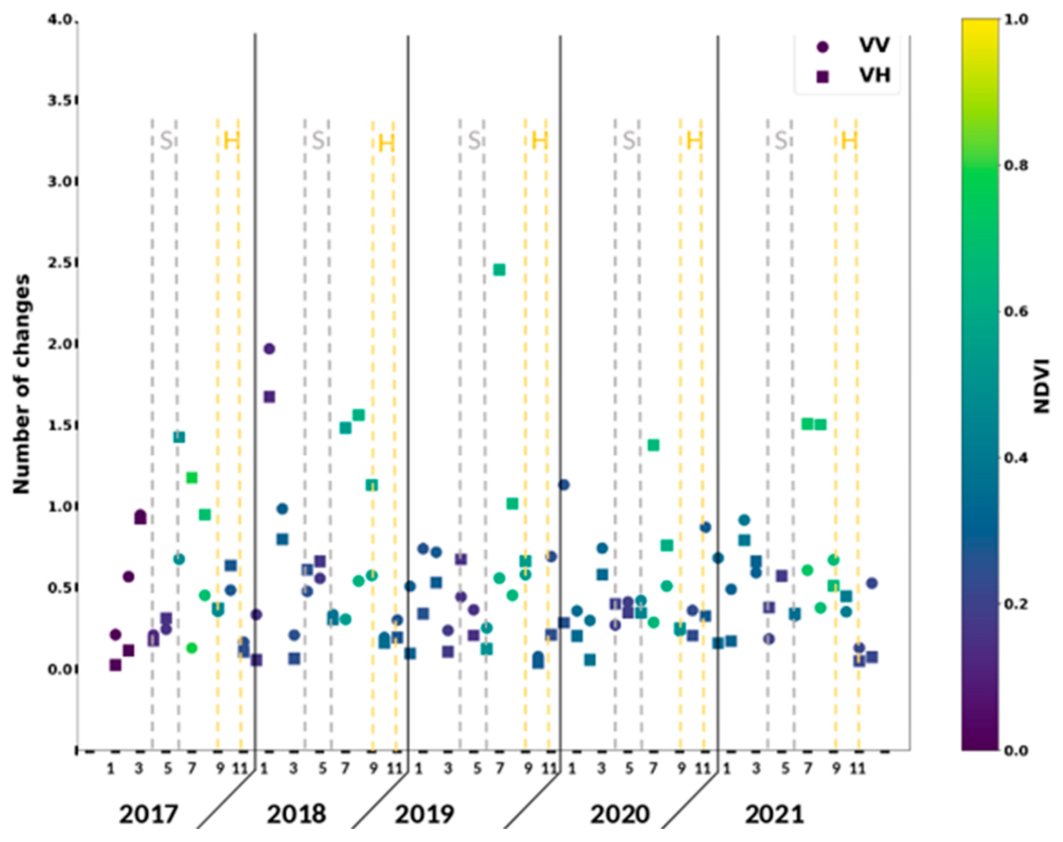
In Figure 5, the NDVI values range from 0 to 0.9, increasing from November to May in all years except 2017, when the increase was limited to April–May. The number of changes based on VH increases from April to May/June (from ~0.5 to ~3.1), coinciding with high NDVI values above 0.7, before sharply decreasing in July to around 0 at the start of the harvest period. This pattern mirrors the Sentinel-1 backscatter changes during fruit development followed by senescence, as Sentinel-1 backscatter for winter rapeseed is known to increase rapidly during fruit development and decrease during the desiccation of rapeseed organs in the fruit maturation period [15,19,59]. The number of changes based on VV follows a similar pattern from January to August, but with fewer changes (ranging from 0 to 2.2). Starting in September, the number of changes based on VV rises (~1–1.5), while the number of changes based on VH remains low, except in 2017.

3.2.2. Monthly Number of Changes and NDVI from the Two Main Summer Crops (Corn, Sunflower)

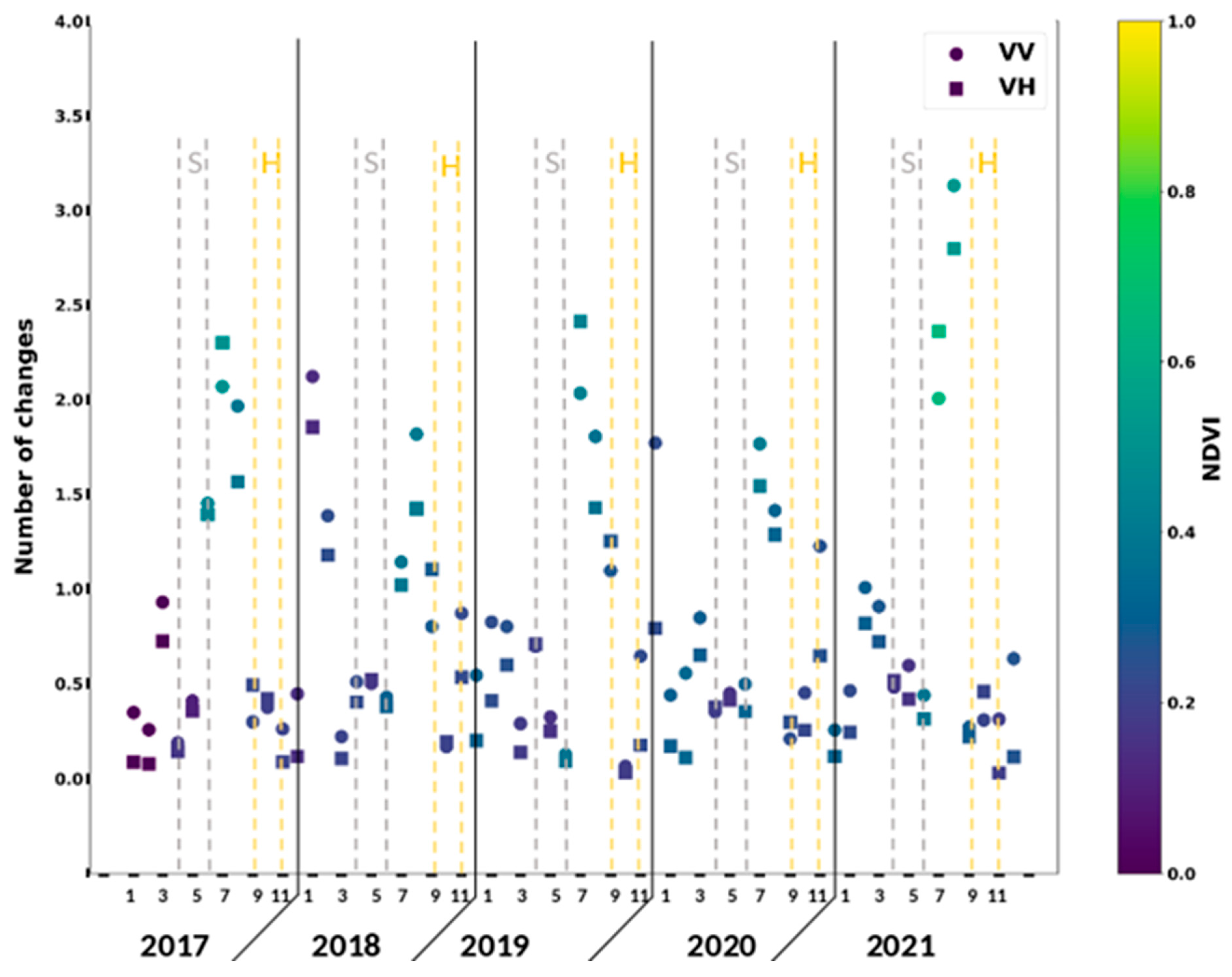
The temporal evolution of maize follows a consistent pattern across the years in both the number of changes and NDVI, except for autumn 2019, as shown in Figure 6. The NDVI values range from 0 in winter to 0.8 during the high-value period from June to August. The number of changes based on VH shows higher values from June to August, during the vegetation growth period, and lower values (<1) during other periods. The number of changes based on VV shows high values during the winter period, ranging from 0 to 2.

Similar to maize, NDVI and the number of changes for sunflower follow comparable patterns across the years (Figure 7). NDVI values range from 0 in winter to 0.6 in August, increasing from June to August. The VH-based number of changes follows a similar pattern, remaining low from autumn to May, then increasing starting in June to reach 1.5~2.3 in July.

Similarly, the number of changes based on VV showed high values in July and August each year (1.5~2). However, it also showed high values during the winter 2017–2018 (2.2) and 2019–2020 (1.8).

3.3. Analysing the Number of Changes for Each Crop Type

In the entire study area, the yearly mean number of changes was computed for each crop type to explore the dynamics of the yearly mean number of changes across the different crop groups and types. In this section, only the spatial differences are studied, not the temporal changes.

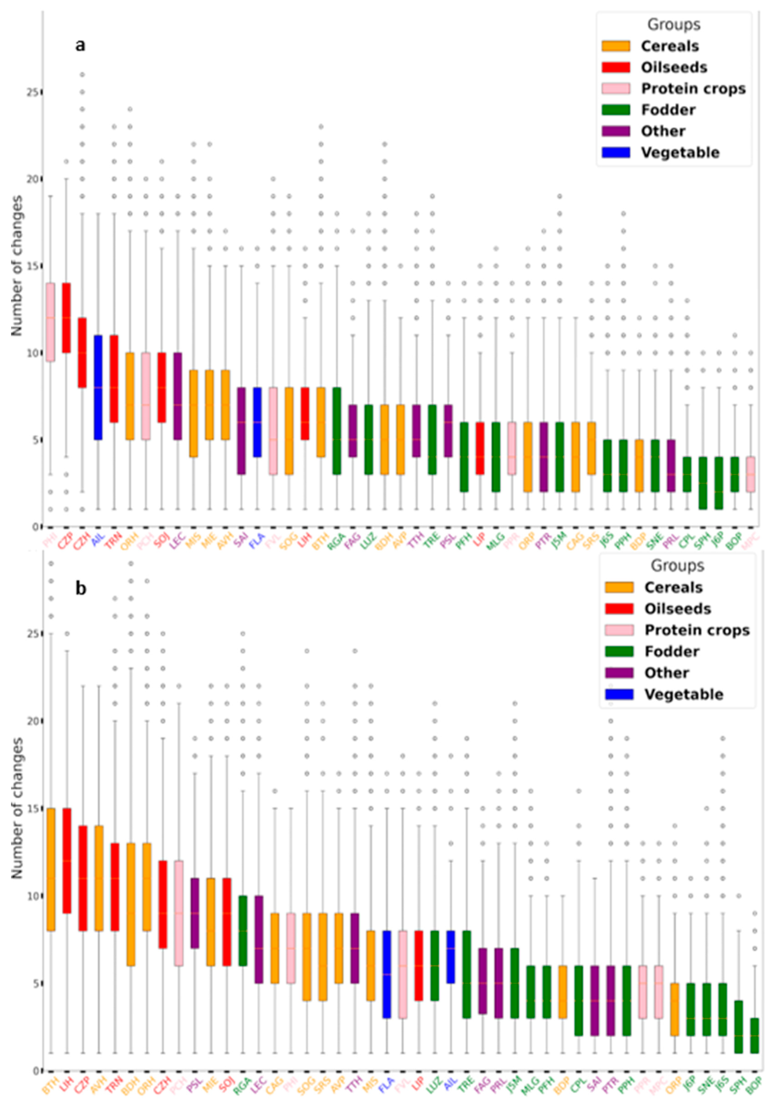
Figure 8 presents the yearly mean number of changes based on VH (a) and VV (b) according to crop type, sorted by the third quartile in 2019, for all the crop types cultivated in the study area. Similar results are obtained for the other years and are presented in the Supplementary Material (Figures S2–S4).

The number of changes significantly varied across crop groups. All fodder types exhibited a median number of changes for VH polarisation lower or equal to 5, the lowest among all crop groups. In contrast, oilseeds showed 83% of their crop types ranging from 7 to 12 changes (spring rapeseed (CZP) > winter rapeseed (CZH) > sunflower (TRN) > soybean (SOJ) > winter non-textile flax (LIH)), with spring non-textile flax (LIP) being at 4.

Cereals showed a wider range of changes and can be divided into two distinct sub-groups. The first sub-group, ranging from 6 to 7 changes (winter barley (ORH), winter oats (AVH), corn (MIE), winter soft wheat (BTH)), represented 41.7% of the total crop types. The second sub-group, with lower third quartiles, ranged from 4 to 5 changes (sorghum (SOG), winter durum wheat (BDH), spring oats (AVP), other cereals (CAG), spring barley (ORP), buckwheat (SRS), spring durum wheat (BDP)).

The protein crop group showed a broad variation in the median yearly number of changes, ranging from 3 to 12. This group consists of five different crop types, with the mix of predominant protein crops and cereals (MPC) being a mixed culture type. Winter pea (PPR) showed the highest number of changes, reaching 12, followed by chickpea (PCH) with 6 changes, fava beans (FVL) at 5, and spring pea (PPR) at 4.

The number of changes observed at VV polarisation exhibited distinct results compared to VH polarisation, although the overall tendencies were similar. For the oilseed group, the number of changes at VV was higher than at VH, ranging from 10 to 12 changes, except for spring non-textural flax (LIP), which only exhibited 6 changes.

Conversely, the fodder group maintained a similar distribution and order for both polarisations, with the following rank: ryegrass (RGA) > alfalfa (LUZ) > clover (TRE), fallow (J5M) > mixture of leguminous plants/forage grass (MLG), forage composed of cereals and protein crops/leguminous forage plants (CPL), PFH, and permanent pasture (PPH), while very low values were observed for temporarily unused agricultural land (SNE), 6-year fallow (J6P), 6-year fallow declared as ecological focus area (J6S), pastoral area (SPH), and wood pasture (BOP).

Cereals, however, presented a higher number of changes at VV than at VH while still forming two distinct sub-groups. The first sub-group (winter soft wheat (BTH), winter oats (AVH), winter durum wheat (BDH), winter barley (ORH), and corn (MIE)) exhibited a range of 8 to 11 changes per year, while the second sub-group (other cereals (CAG), spring oats (AVP), corn (MIS), and sorghum (SOG)) had a range from 5 to 6 changes annually. The number of changes in spring durum wheat (BDP) and spring oats (ORP) remained consistently low.

In the protein crop group, winter peas (PHI) showed a variation between polarisations, with 12 changes at VH and 7 at VV, while chickpeas (PCH) showed 6 changes at VH and 9 at VV. Fava beans (FVL) exhibited a constant value of 5 changes across both polarisations.

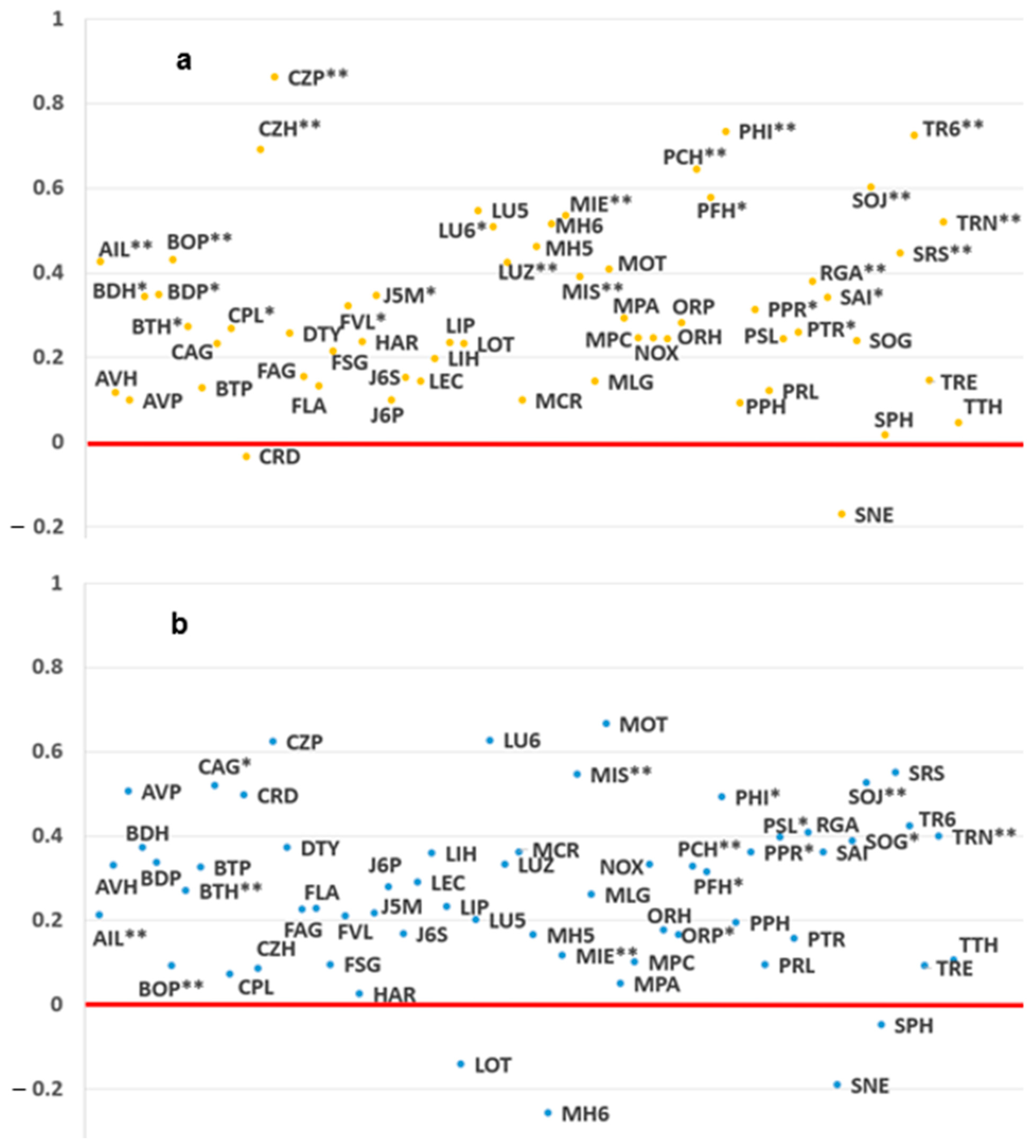
Figure 9 presents the correlation coefficients between the monthly mean NDVI and the number of monthly changes based on (a) VH and (b) VV. This figure highlights distinct levels in correlations between the number of changes at VH polarisation and NDVI, in contrast to those at VV polarisation and NDVI. The number of changes at VH polarisation was positively correlated with NDVI for 46 crop types, whereas the number of changes based on VV was negatively correlated with NDVI for 38 culture types.

Sixteen crop types showed a significant positive correlation between the number of changes at VH polarisation and NDVI, five of which showed a correlation coefficient R greater than 0.6: corn (MIS), parsley (PSL), soybean (SOJ), TR5, and sunflower (TRN). Ten culture types showed a moderate positive VH correlation (0.4 < R < 0.6), five of which were statistically significant. Six culture types showed a significant low positive correlation (0.2 < R < 0.4), and two showed a significant moderate negative correlation (wood pasture (BOP), winter soft wheat (BTH), R < −0.4).

Regarding the correlation between the monthly mean number of changes at VV polarisation and NDVI, two crops (winter durum and winter soft wheats (BDH, BTH)) exhibited a significant strong negative correlation (R < −0.6), three showed a significant moderate negative correlation (winter non-textile flax (LIH), winter barley, PSL, −0.6 < R < −0.4), and one showed a significant moderate positive correlation (soybean (SOJ), 0.4 < R < 0.6) while another one showed a significant strong positive correlation (sunflower (TRN), R > 0.6). Ten cultures showed a significant low negative correlation (−0.4 < R < −0.2).

The groups of crops were also analysed and compared in

Table 3. A comparative table of the groups of crops: cereals, oilseeds, protein, fodder, other, and vegetable in terms of the difference in the number of changes. The confidence intervals (CI) of 2.5 and 97.5% are shown.

Group of Crop A	Group of Crop B	Effect Size	CI 2.5	CI 97.5
Cereals	Oilseeds	0.45	0.44	0.46
Cereals	Protein crops	2.33	2.3	2.37
Cereals	Fodder	4.56	4.55	4.57
Cereals	Other	1.24	1.11	1.36
Cereals	Vegetable	3.11	3.03	3.19
Oilseeds	Protein crops	1.88	1.84	1.92
Oilseeds	Fodder	4.11	4.1	4.12
Oilseeds	Other	0.78	0.66	0.91
Oilseeds	Vegetable	2.66	2.58	2.74
Protein crops	Fodder	2.23	2.2	2.27
Protein crops	Other	−1.1	−1.23	−0.98
Protein crops	Vegetable	0.77	0.68	0.86
Fodder	Other	−3.33	−3.45	−3.21
Fodder	Vegetable	−1.46	−1.54	−1.38
Other	Vegetable	1.87	1.71	2

. All groups were found to be statistically different with high degrees of significance. These high degrees of significance may be attributed to the large sample sizes of pixel populations, as even small differences can become statistically significant due to the number of occurrences. The effect size and confidence interval at 2.5 and 97.5% were computed using a bootstrap based on a block approach, with 500 iterations (at the parcel level). It is possible to see that the cereal and oilseed groups have the highest mean number of changes and are similar to a 0.45 mean yearly number of changes difference. They are followed by the ‘Other’ group and protein crops, with respective 1.24 and 2.33 differences. All groups showed significant differences from each other in terms of yearly mean number of changes (from an absolute 0.44 to 4.57 changes).

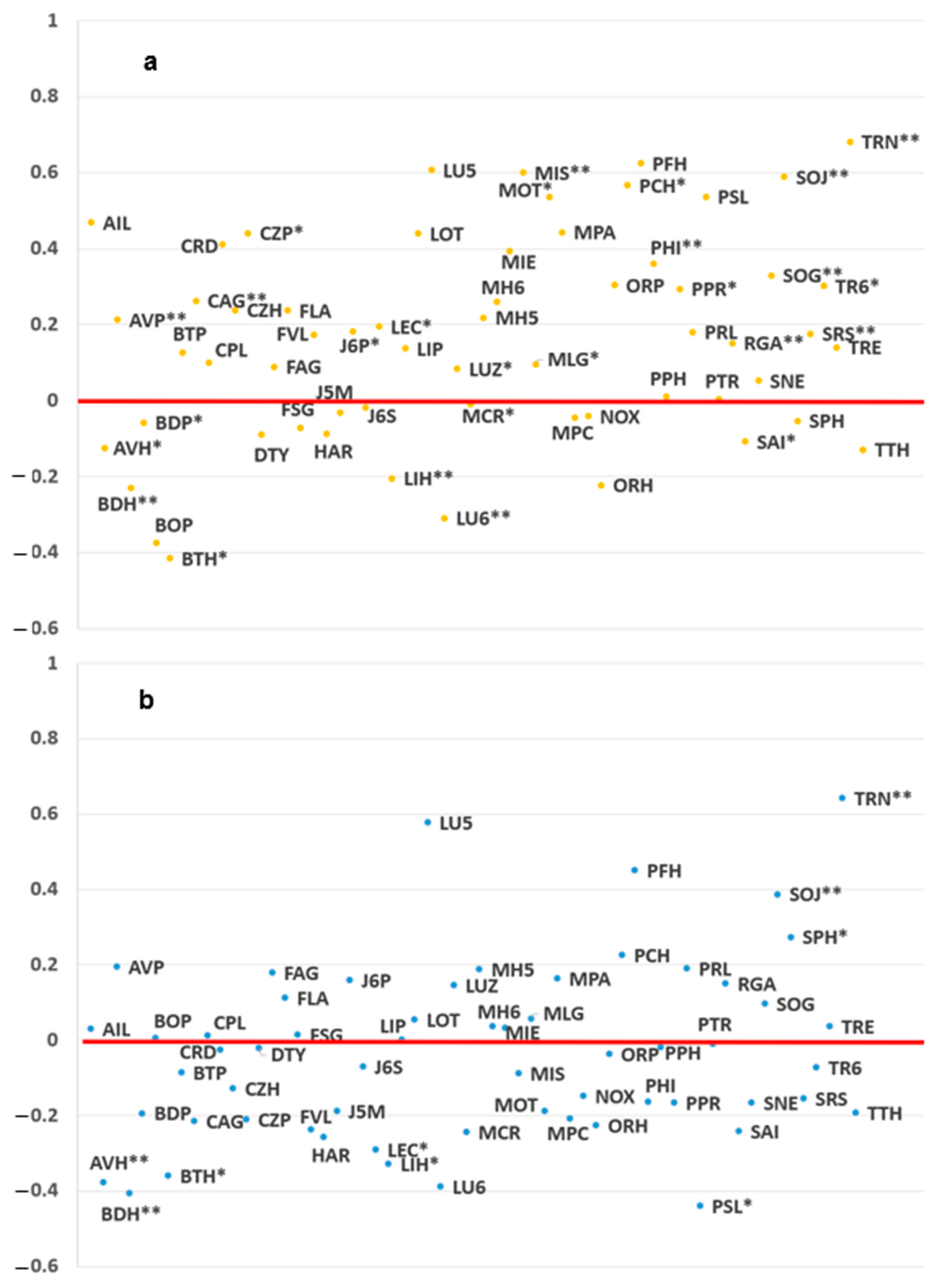
Figure 10a shows the correlation between VH-based monthly mean number of changes and VH backscatter according to crop type. Twenty-three crop types show significant correlations, with one showing a correlation higher than 0.8, spring rapeseed (CZP, 0.67). Five have a correlation between 0.6 and 0.8: winter peas (PHI, 0.73), clover sown for the 2016 harvest (TR6, 0.72), winter rapeseed (CZH, 0.69), chickpea (PCH,0.65), and soybean (SOJ, 0.6).

Eight crop types show a significant moderate correlation (between 0.4 and 0.6): other winter forage peas (PFH, 0.58), corn (MIE, 0.54), sunflower (TRN, 0.52), alfalfa sown for the 2016 harvest (LU6, 0.51), buckwheat (SRS, 0.45), pasture wood (BOP, 0.43), garlic (AIL, 0.43), and alfalfa (LUZ, 0.42). No anticorrelation was found between the number of changes and the backscatter value.

Figure 10b shows the correlation between VV-based monthly mean number of changes and VV backscatter according to crop type. Fifteen crop types show significant correlations, with only 4 showing a correlation higher than 0.4: corn (MIS, 0.54), soybean (SOJ, 0.53), other cereals (CAG, 0.52), and winter peas (PHI, 0.49). No significant anticorrelation was found.

4. Discussion

This study examined the applicability of the cumulative sum (CuSum) change point detection method using Sentinel-1 data as a near-real-time approach for monitoring soil work and vegetation growth in crop fields. The findings were extended to a 6 km radius circle encompassing all other crop fields (61) in the region.

In both Lamasquère and Auradé, the number of changes based on VH polarisation was positively correlated with high NDVI values, a pattern consistent with results observed for the other fields of the area. This positive correlation suggests that the VH-based number of changes increases as vegetation grows and when its cover becomes denser, corresponding to higher NDVI values. This result agrees with the statement of [60]: the VH polarisation backscatter is primarily controlled by volume scattering within the canopy, as vegetation structure dominates the radar response once canopy development progresses.

In contrast, the VV-based number of changes showed no clear trend in relation to vegetation index, remaining high during both high and low NDVI periods according to the crop type studied. This partially supports the negative correlation observed for VV-based changes across the study area as periods of low NDVI are longer than periods of high NDVI. These contrasting results are in agreement with the physical interpretation proposed by [61], which describes VH backscatter to be generally more sensitive to vegetation-related volume scattering, whereas VV backscatter is more influenced by surface scattering components.

Two drought events were present during the study period: from May 2018 to April 2019 and in 2020, according to Meteo-France [58]. However, no increase in the number of changes was found for the major crops in the region during these events, suggesting that other factors may have influenced the changes. Notably, no clear correlation was found between soil work events (such as tillage or stubble cultivation) and the number of changes detected. This discrepancy may be due to the temporal resolution of the methodology, which operates at a monthly scale, potentially missing short-term changes associated with soil work activities. Further work is needed to comprehend the spatial dynamic of changes associated with the dates of soil activities as the monthly scale has proven insufficient.

The study also analysed the number of changes for the two main winter crops (winter soft wheat and winter rapeseed), summer crops (maize and soybean), and permanent grassland present in the area. The relationship between the number of changes and NDVI varied by crop type: a strong negative correlation was observed for winter wheat as low numbers of change values were associated with high NDVI values. This is consistent with previous studies [19,62,63,64], which have shown that Sentinel-1 backscatter decreases as wheat grows, impacting the detection of changes during this period. The limited number of changes detected during the growth phase of wheat can be attributed to this backscatter saturation effect, particularly in the short time series used for each CuSum-NRT iteration.

The analysis of the correlation coefficient between NDVI and the monthly mean number of changes according to crop type and polarisation showed interesting results. VH-based number of changes was predominantly correlated positively with NDVI, which is consistent with the hypothesis that VH can be used to monitor vegetation growth. Contrarily, the VV-based number of changes was mostly negatively correlated with NDVI, which means that a higher number of changes was found during periods without vegetation. This result is consistent with [61], as the VV polarisation is known to fluctuate with surface variations. To analyse changes in vegetation, the VV polarisation should not be used with CuSum.

The correlations between the monthly mean VV backscatter and the VV-based monthly mean number of changes varied according to the crop type. No significant high correlation was found, and only a few crop types had a moderate correlation: the information about the VV-based monthly mean number of changes is complementary to that of VV backscatter. Contrarily, many crop types show a high correlation (>0.6) between the monthly mean VH backscatter and the VH-based monthly mean number of changes. However, the crop types showing a high correlation are not the same as those that show a high correlation with NDVI. The VH-based monthly mean number of changes gives complementary information to NDVI and the monthly mean VH backscatter.

5. Conclusions

This publication aimed to assess the potential of the cumulative sum algorithm (CuSum) near-real-time (NRT) method based on Sentinel-1 time series of images for monitoring crops at both field and crop levels in Southwestern France between 2017 and 2021. The monthly mean number of changes derived from this method was analysed in relation to NDVI derived from Sentinel-2 with less than 30% cloud cover, as well as in situ measurements such as precipitation or agricultural practices from the Lamasquère and Auradé Integrated Carbon Observation System stations.

The results indicated that the monthly mean number of changes varied according to the polarisations, crop types, growth stages, and climate conditions. However, different soil work in Lamasquère and Auradé did not appear to significantly affect the monthly mean number of changes: the monthly grain of the temporal resolution may be too low to differentiate the changes due to soil work or phenology states from other changes. Further work is needed at intra-parcel resolution to estimate the spatial detection of a single soil operation, at date-of-change resolution.

The analysis showed that the VH-based number of changes was positively correlated with NDVI for 16 different crops (Rmax = 0.73), indicating a strong association between vegetation growth and this polarisation. In contrast, the VV-based number of changes was predominantly negatively correlated with NDVI, with 12 significant negative correlations. Notably, winter wheat (both hard and soft) exhibited the highest negative correlations for the VV-based number of changes (R = −0.69 in both cases).

Furthermore, the different groups of crops (cereals, oilseeds, protein crops, fodder, vegetables, and others) displayed statistically significant differences (0.45 to 4.57 changes) in their yearly number of changes, with cereals and oilseeds showing higher values than the other groups.

Lastly, the CuSum-NRT method was found to have a poor correlation with the VV monthly mean backscatter (R_global = 0.25) and a strong correlation with the VH monthly mean backscatter (R_global = 0.61). Depending on the crop type, the CuSum-NRT information is complementary to NDVI and polarisation backscatter for both VV and VH.

Overall, this study confirms that the CuSum change point detection method is a promising approach for monitoring vegetation dynamics at the field scale using Sentinel-1 data. It adds information complementary to backscatter and NDVI. Contrary to NDVI-based monitoring, the use of Sentinel-1 allows for continuous crop monitoring even during cloudy seasons. However, further research is needed to refine the methodology, particularly in relation to better analysing the effects of soil work and other short-term land management activities to improve its applicability or to link changes with biomass increase, change of phenology state.

References

1. Buckley, C.; Carney, P. The potential to reduce the risk of diffuse pollution from agriculture while improving economic performance at farm level. Environ. Sci. Policy 2013, 25, 118–126. [Google Scholar] [CrossRef] [Scilit]
2. Foley, J.A.; DeFries, R.; Asner, G.P.; Barford, C.; Bonan, G.; Carpenter, S.R.; Chapin, F.S.; Coe, M.T.; Daily, G.C.; Gibbs, H.K.; et al. Global consequences of land use. Science 2005, 309, 570–574. [Google Scholar] [CrossRef] [Scilit]
3. Steele-Dunne, S.C.; McNairn, H.; Monsivais-Huertero, A.; Judge, J.; Liu, P.-W.; Papathanassiou, K. Radar remote sensing of agricultural canopies: A review. IEEE J. Sel. Top. Appl. Earth Obs. Remote Sens. 2017, 10, 2249–2273. [Google Scholar] [CrossRef] [Scilit]
4. Mandal, N.; Das, D.K.; Sahoo, R.N.; Adak, S.; Kumar, A.; Viswanathan, C.; Mukherjee, J.; Rajashekara, H.; Ranjan, R.; Das, B. Assessing rice blast disease severity through hyperspectral remote sensing. J. Agrometeorol. 2022, 24, 241–248. [Google Scholar] [CrossRef] [Scilit]
5. Gao, F.; Zhang, X. Mapping Crop Phenology in Near Real-Time Using Satellite Remote Sensing: Challenges and Opportunities. J. Remote Sens. 2021, 2021, 8379391. [Google Scholar] [CrossRef] [Scilit]
6. Mestre-Quereda, A.; Lopez-Sanchez, J.M.; Vicente-Guijalba, F.; Jacob, A.W.; Engdahl, M.E. Time-Series of Sentinel-1 Interferometric Coherence and Backscatter for Crop-Type Mapping. IEEE J. Sel. Top. Appl. Earth Obs. Remote Sens. 2020, 13, 4070–4084. [Google Scholar] [CrossRef] [Scilit]
7. Woźniak, E.; Rybicki, M.; Kofman, W.; Aleksandrowicz, S.; Wojtkowski, C.; Lewiński, S.; Bojanowski, J.; Musiał, J.; Milewski, T.; Slesiński, P.; et al. Multi-temporal phenological indices derived from time series Sentinel-1 images to country-wide crop classification. Int. J. Appl. Earth Obs. Geoinf. 2022, 107, 102683. [Google Scholar] [CrossRef] [Scilit]
8. Baup, F.; Fieuzal, R.; Battista, C.; Ramiakatrarivony, H.; Tournier, L.; Diarra, S.-F.; Riazanoff, S.; Frappart, F. The Capabilities of Optical and C-Band Radar Satellite Data to Detect and Understand Faba Bean Phenology over a 6-Year Period. Remote Sens. 2025, 17, 1933. [Google Scholar] [CrossRef] [Scilit]
9. Attema, E.P.W.; Ulaby, F.T. Vegetation modeled as a water cloud. Radio Sci. 1978, 13, 357–364. [Google Scholar] [CrossRef] [Scilit]
10. McNairn, H.; Shang, J. A review of multitemporal synthetic aperture radar (SAR) for crop monitoring. In Multitemporal Remote Sensing: Methods and Applications; Springer International Publishing: Cham, Switzerland, 2016; pp. 317–340. [Google Scholar]
11. Weiss, M.; Jacob, F.; Duveiller, G. Remote sensing for agricultural applications: A meta-review. Remote Sens. Environ. 2020, 236, 111402. [Google Scholar] [CrossRef] [Scilit]
12. Betbeder, J.; Fieuzal, R.; Baup, F. Assimilation of LAI and dry biomass data from optical and SAR images into an agro-meteorological model to estimate soybean yield. IEEE J. Sel. Top. Appl. Earth Obs. Remote Sens. 2016, 9, 2540–2553. [Google Scholar] [CrossRef] [Scilit]
13. Fieuzal, R.; Sicre, C.M.; Baup, F. Estimation of corn yield using multi-temporal optical and radar satellite data and artificial neural networks. Int. J. Appl. Earth Obs. Geoinf. 2017, 57, 14–23. [Google Scholar] [CrossRef] [Scilit]
14. Fieuzal, R.; Sicre, C.M.; Baup, F. Estimation of sunflower yield using a simplified agrometeorological model controlled by optical and SAR satellite data. IEEE J. Sel. Top. Appl. Earth Obs. Remote Sens. 2017, 10, 5412–5422. [Google Scholar] [CrossRef] [Scilit]
15. Fieuzal, R.; Baup, F.; Marais-Sicre, C. Monitoring wheat and rapeseed by using synchronous optical and radar satellite data—From temporal signatures to crop parameters estimation. EARSeL Adv. Remote Sens. 2013, 2, 162–180. [Google Scholar] [CrossRef]
16. Baup, F.; Ameline, M.; Fieuzal, R.; Frappart, F.; Corgne, S.; Berthoumieu, J.-F. Temporal evolution of corn mass production based on agro-meteorological modelling controlled by satellite optical and SAR images. Remote Sens. 2019, 11, 1978. [Google Scholar] [CrossRef] [Scilit]
17. Ameline, M.; Fieuzal, R.; Betbeder, J.; Berthoumieu, J.F.; Baup, F. Estimation of Corn Yield by Assimilating SAR and Optical Time Series into a Simplified Agro-Meteorological Model: From Diagnostic to Forecast. IEEE J. Sel. Top. Appl. Earth Obs. Remote Sens. 2018, 11, 4747–4760. [Google Scholar] [CrossRef] [Scilit]
18. Gorrab, A.; Ameline, M.; Albergel, C.; Baup, F. Use of Sentinel-1 Multi-Configuration and Multi-Temporal Series for Monitoring Parameters of Winter Wheat. Remote Sens. 2021, 13, 553. [Google Scholar] [CrossRef] [Scilit]
19. Mercier, A.; Betbeder, J.; Baudry, J.; Le Roux, V.; Spicher, F.; Lacoux, J.; Roger, D.; Hubert-Moy, L. Evaluation of Sentinel-1 & 2 time series for predicting wheat and rapeseed phenological stages. ISPRS J. Photogramm. Remote Sens. 2020, 163, 231–256. [Google Scholar]
20. Senaras, C.; Grady, M.; Rana, A.S.; Nieto, L.; Ciampitti, I.; Holden, P.; Davis, T.; Wania, A. Detection of Maize Crop Phenology Using Planet Fusion. Remote Sens. 2024, 16, 2730. [Google Scholar] [CrossRef] [Scilit]
21. Htitiou, A.; Möller, M.; Riedel, T.; Beyer, F.; Gerighausen, H. Towards Optimising the Derivation of Phenological Phases of Different Crop Types over Germany Using Satellite Image Time Series. Remote Sens. 2024, 16, 3183. [Google Scholar] [CrossRef] [Scilit]
22. Harfenmeister, K.; Itzerott, S.; Weltzien, C.; Spengler, D. Detecting Phenological Development of Winter Wheat and Winter Barley Using Time Series of Sentinel-1 and Sentinel-2. Remote Sens. 2021, 13, 5036. [Google Scholar] [CrossRef] [Scilit]
23. Tran, K.H.; Zhang, X.; Zhang, H.K.; Shen, Y.; Ye, Y.; Liu, Y.; Gao, S.; An, S. A transformer-based model for detecting land surface phenology from the irregular harmonized Landsat and Sentinel-2 time series across the United States. Remote Sens. Environ. 2025, 320, 114656. [Google Scholar] [CrossRef] [Scilit]
24. Yang, J.; Shi, H.; Xie, Q.; Lopez-Sanchez, J.M.; Peng, X.; Yu, J.; Chen, L. Crop Phenology Estimation in Rice Fields Using Sentinel-1 GRD SAR Data and Machine Learning-Aided Particle Filtering Approach. Int. Arch. Photogramm. Remote Sens. Spat. Inf. Sci. 2024, XLVIII-1–2024, 799–804. [Google Scholar] [CrossRef] [Scilit]
25. Dhillon, M.S.; Dahms, T.; Kuebert-Flock, C.; Rummler, T.; Arnault, J.; Steffan-Dewenter, I.; Ullmann, T. Integrating random forest and crop modeling improves the crop yield prediction of winter wheat and oil seed rape. Front. Remote Sens. 2023, 3, 1010978. [Google Scholar] [CrossRef] [Scilit]
26. Lobert, F.; Löw, J.; Schwieder, M.; Gocht, A.; Schlund, M.; Hostert, P.; Erasmi, S. A deep learning approach for deriving winter wheat phenology from optical and SAR time series at field level. Remote Sens. Environ. 2023, 298, 113800. [Google Scholar] [CrossRef] [Scilit]
27. Valcarce-Diñeiro, R.; Arias-Pérez, B.; Lopez-Sanchez, J.M.; Sánchez, N. Multi-Temporal Dual- and Quad-Polarimetric Synthetic Aperture Radar Data for Crop-Type Mapping. Remote Sens. 2019, 11, 1518. [Google Scholar] [CrossRef] [Scilit]
28. Wang, L.; Wang, T.; Ma, H.; Lu, P.; Sun, W.; Fan, L.; Wang, H.; Wu, Y.; Wang, Y. Time-Series SAR Monitoring of Rice in Multiple Cropping Modes Combining Statistical and Phenological Characteristics. IEEE Trans. Geosci. Remote Sens. 2024, 62, 4411811. [Google Scholar] [CrossRef] [Scilit]
29. Mimić, G.; Mishra, A.K.; Marković, M.; Živaljević, B.; Pavlović, D.; Marko, O. Machine Learning-Based Harvest Date Detection and Prediction Using SAR Data for the Vojvodina Region (Serbia). Sensors 2025, 25, 2239. [Google Scholar] [CrossRef] [Scilit]
30. Yue, J.; Yao, Y.; Shen, J.; Li, T.; Xu, N.; Feng, H.; Wei, Y.; Xu, X.; Lin, Y.; Guo, W.; et al. Winter wheat harvest detection via Sentinel-2 MSI images. Int. J. Remote Sens. 2025, 46, 2482–2500. [Google Scholar] [CrossRef] [Scilit]
31. Masiliūnas, D.; Tsendbazar, N.-E.; Herold, M.; Verbesselt, J. BFAST Lite: A Lightweight Break Detection Method for Time Series Analysis. Remote Sens. 2021, 13, 3308. [Google Scholar] [CrossRef] [Scilit]
32. Saxena, R.; Watson, L.T.; Wynne, R.H.; Brooks, E.B.; Thomas, V.A.; Zhiqiang, Y.; Kennedy, R.E. Towards a polyalgorithm for land use change detection. ISPRS J. Photogramm. Remote Sens. 2018, 144, 217–234. [Google Scholar] [CrossRef] [Scilit]
33. Hamunyela, E.; Roşca, S.; Mirt, A.; Engle, E.; Herold, M.; Gieseke, F.; Verbesselt, J. Implementation of BFAST monitor Algorithm on Google Earth Engine to support large-area and sub-annual change monitoring using earth observation data. Remote Sensing 2020, 12, 2953. [Google Scholar] [CrossRef] [Scilit]
34. Dua, B.; Yuanb, Z. A New Method for Automatic Deforestation Detection: Change Point Detection and Machine Learning. Int. Core J. Eng. 2023, 9, 182–192. [Google Scholar]
35. Reiche, J.; Hamunyela, E.; Verbesselt, J.; Hoekman, D.; Herold, M. Improving near-real time deforestation monitoring in tropical dry forests by combining dense Sentinel-1 time series with Landsat and ALOS-2 PALSAR-2. Remote Sens. Environ. 2018, 204, 147–161. [Google Scholar] [CrossRef] [Scilit]
36. Hamunyela, E.; Verbesselt, J.; Herold, M. Using spatial context to improve early detection of deforestation from Landsat time series. Remote Sens. Environ. 2016, 172, 126–138. [Google Scholar] [CrossRef] [Scilit]
37. Ruiz-Ramos, J.; Marino, A.; Berardi, A.; Hardy, A.; Simpson, M. Characterization of Natural Wetlands with Cumulative Sums of Polarimetric Sar Timeseries. In Proceedings of the 2021 IEEE International Geoscience and Remote Sensing Symposium IGARSS, Brussels, Belgium, 11–16 July 2021; IEEE: Piscataway, NJ, USA, 2021; pp. 5899–5902. [Google Scholar]
38. Mistry, J.; Jafferally, D.; Ruiz-Ramos, J.; Xavier, R.; Albert, G.; Berardi, A.; Mendonca, S.; Robertson, B. COVID-19 Impacts on Indigenous Food Sovereignty, Livelihoods and Biodiversity, Guyana. 2021. Available online: www.cobracollective.org/resources (accessed on 11 November 2024).
39. Ruiz-Ramos, J.; Marino, A.; Boardman, C.; Suarez, J. Continuous forest monitoring using cumulative sums of sentinel-1 timeseries. Remote Sens. 2020, 12, 3061. [Google Scholar] [CrossRef] [Scilit]
40. Ruiz-Ramos, J.; Marino, A.; Boardman, C.P. Using Sentinel 1-Sar for Monitoring Long Term Variation in Burnt Forest Areas. In Proceedings of the IGARSS 2018—2018 IEEE International Geoscience and Remote Sensing Symposium, Valencia, Spain, 22–27 July 2018; pp. 4901–4904. [Google Scholar]
41. Muro, J.; Canty, M.; Conradsen, K.; Hüttich, C.; Nielsen, A.A.; Skriver, H.; Remy, F.; Strauch, A.; Thonfeld, F.; Menz, G. Short-Term Change Detection in Wetlands Using Sentinel-1 Time Series. Remote Sens. 2016, 8, 795. [Google Scholar] [CrossRef] [Scilit]
42. Ygorra, B.; Frappart, F.; Wigneron, J.; Moisy, C.; Catry, T.; Baup, F.; Hamunyela, E.; Riazanoff, S. Monitoring loss of tropical forest cover from Sentinel-1 time-series: A CuSum-based approach. Int. J. Appl. Earth Obs. Geoinf. 2021, 103, 102532. [Google Scholar] [CrossRef] [Scilit]
43. Ygorra, B.; Frappart, F.; Wigneron, J.-P.; Moisy, C.; Catry, T.; Baup, F.; Hamunyela, E.; Riazanoff, S. Deforestation Monitoring Using Sentinel-1 SAR Images in Humid Tropical Areas. In Proceedings of the 2021 IEEE International Geoscience and Remote Sensing Symposium IGARSS, Brussels, Belgium, 11–16 July 2021; pp. 5957–5960. [Google Scholar] [CrossRef] [Scilit]
44. Ygorra, B.; Frappart, F.; Wigneron, J.-P.; Moisy, C.; Pillot, B.; Puiseux, J.; Riazanoff, S. Classification and Deforestation Monitoring Using Sentinel-1 C-SAR Images in a Temperate Exploited Pine Forest. In Proceedings of the IGARSS 2022—2022 IEEE International Geoscience and Remote Sensing Symposium, Kuala Lumpur, Malaysia, 17–22 July 2022; IEEE: Piscataway, NJ, USA, 2022; pp. 691–694. [Google Scholar]
45. Pfefer, A.; Ygorra, B.; Frappart, F.; Demarchi, G.; Pillot, B.; Subervie, J.; Wigneron, J.-P.; Catry, T. How Sentinel-1 timeseries can improve the implementation of conservation programs in Brazil. Remote Sens. Appl. Soc. Environ. 2024, 35, 101241. [Google Scholar] [CrossRef] [Scilit]
46. Ygorra, B.; Frappart, F.; Wigneron, J.-P.; Catry, T.; Pillot, B.; Riazanoff, S. Sentinel-1 Based Cusum Capabilities as a Forest/Non-Forest Mask in Tropical Areas. In Proceedings of the IGARSS 2023—2023 IEEE International Geoscience and Remote Sensing Symposium, Pasadena, CA, USA, 16–21 July 2023; pp. 6228–6230. [Google Scholar] [CrossRef] [Scilit]
47. Ygorra, B.; Frappart, F.; Wigneron, J.-P.; Christophe, M.; Catry, T.; Pillot, B.; Courtalon, J.; Kharlanova, A.; Riazanoff, S.; Interactions Sol Plante Atmosphère (UMR ISPA); et al. Corrigendum to “ReCuSum: A polyvalent method to monitor tropical forest disturbances” [ISPRS J. Photogramm. Rem. Sens. 203 (2023) 358–372]. ISPRS J. Photogramm. Remote Sens. 2024, 211, 298. [Google Scholar] [CrossRef] [Scilit]
48. Ygorra, B.; Frappart, F.; Wigneron, J.-P.; Catry, T.; Pillot, B.; Pfefer, A.; Courtalon, J.; Riazanoff, S. A near-real-time tropical deforestation monitoring algorithm based on the CuSum change detection method. Front. Remote Sens. 2024, 5, 1416550. [Google Scholar] [CrossRef] [Scilit]
49. Ouin, A.; Andrieu, E.; Vialatte, A.; Balent, G.; Barbaro, L.; Blanco, J.; Ceschia, E.; Clement, F.; Fauvel, M.; Gallai, N.; et al. Building a shared vision of the future for multifunctional agricultural landscapes. Lessons from a long term socio-ecological research site in south-western France. In Advances in Ecological Research; Elsevier: Amsterdam, The Netherlands, 2021; Volume 65, pp. 57–106. [Google Scholar]
50. Gaillardet, J.; Braud, I.; Hankard, F.; Anquetin, S.; Bour, O.; Dorfliger, N.; de Dreuzy, J.; Galle, S.; Galy, C.; Gogo, S.; et al. OZCAR: The French network of critical zone observatories. Vadose Zone J. 2018, 17, 1–24. [Google Scholar] [CrossRef] [Scilit]
51. Franz, D.; Acosta, M.; Altimir, N.; Arriga, N.; Arrouays, D.; Aubinet, M.; Aurela, M.; Ayres, E.; López-Ballesteros, A.; Barbaste, M.; et al. Towards long-term standardised carbon and greenhouse gas observations for monitoring Europe’s terrestrial ecosystems: A review. Int. Agrophysics 2018, 32, 439–455. [Google Scholar] [CrossRef] [Scilit]
52. Torres, R.; Snoeij, P.; Geudtner, D.; Bibby, D.; Davidson, M.; Attema, E.; Potin, P.; Rommen, B.; Floury, N.; Brown, M.; et al. GMES Sentinel-1 mission. Remote Sens. Environ. 2012, 120, 9–24. [Google Scholar] [CrossRef] [Scilit]
53. Piantanida, R.; Miranda, N.; Franceschi, N.; Meadows, P. Thermal Denoising of Products Generated by the S-1 IPF, Issue 1.1. 2017. Available online: https://sentinels.copernicus.eu/documents/247904/2142675/Thermal-Denoising-of-Products-Generated-by-Sentinel-1-IPF.pdf (accessed on 1 June 2023).
54. Small, D. Flattening gamma: Radiometric terrain correction for SAR imagery. IEEE Trans. Geosci. Remote Sens. 2011, 49, 3081–3093. [Google Scholar] [CrossRef] [Scilit]
55. Reigber, A.; del Campo Becerra, G.M.; Jäger, M. PyRAT: A Flexible SAR Postprocessing Toolbox. In Proceedings of the ESA POLinSAR Workshop, Frascati, Italy, 28 January–1 February 2019. [Google Scholar]
56. Drusch, M.; Del Bello, U.; Carlier, S.; Colin, O.; Fernandez, V.; Gascon, F.; Hoersch, B.; Isola, C.; Laberinti, P.; Martimort, P.; et al. Sentinel-2: ESA’s Optical High-Resolution Mission for GMES Operational Services. Remote Sens. Environ. 2012, 120, 25–36. [Google Scholar] [CrossRef] [Scilit]
57. Manogaran, G.; Lopez, D. Spatial cumulative sum algorithm with big data analytics for climate change detection. Comput. Electr. Eng. 2018, 65, 207–221. [Google Scholar] [CrossRef] [Scilit]
58. Météo-France. Bilan Définitif de L’été. 2020. Available online: https://meteofrance.fr/sites/meteofrance.fr/files/files/editorial/bilan_definitif_ete_2020.pdf (accessed on 1 January 2021).
59. Allies, A.; Roumiguié, A.; Dejoux, J.-F.; Fieuzal, R.; Jacquin, A.; Veloso, A.; Champolivier, L.; Baup, F. Evaluation of multiorbital SAR and multisensor optical data for empirical estimation of rapeseed biophysical parameters. IEEE J. Sel. Top. Appl. Earth Obs. Remote Sens. 2021, 14, 7268–7283. [Google Scholar] [CrossRef] [Scilit]
60. Baup, F.; Fieuzal, R.; Ygorra, B.; Frappart, F.; Riazanoff, S.; Martin-Comte, A.; Gorrab, A. 6-Years of SAR (Sentinel-1) and Optical (Sentinel-2, Landsat-8) Acquisitions over Agricultural Surfaces in Southwestern France. Remote Sens. 2025; in review.
61. Kellndorfer, J. Using SAR data for mapping deforestation and forest degradation. In THE SAR HANDBOOK Comprehensive Methodologies for Forest Monitoring and Biomass Estimation; ServirGlobal: Huntsville, AL, USA, 2019; pp. 65–79. [Google Scholar]
62. Vreugdenhil, M.; Wagner, W.; Bauer-Marschallinger, B.; Pfeil, I.; Teubner, I.; Rüdiger, C.; Strauss, P. Sensitivity of Sentinel-1 Backscatter to Vegetation Dynamics: An Austrian Case Study. Remote Sens. 2018, 10, 1396. [Google Scholar] [CrossRef] [Scilit]
63. Khabbazan, S.; Vermunt, P.; Steele-Dunne, S.; Arntz, L.R.; Marinetti, C.; van der Valk, D.; Iannini, L.; Molijn, R.; Westerdijk, K.; van der Sande, C. Crop Monitoring Using Sentinel-1 Data: A Case Study from The Netherlands. Remote Sens. 2019, 11, 1887. [Google Scholar] [CrossRef] [Scilit]
64. Vavlas, N.-C.; Waine, T.W.; Meersmans, J.; Burgess, P.J.; Fontanelli, G.; Richter, G.M. Deriving Wheat Crop Productivity Indicators Using Sentinel-1 Time Series. Remote Sens. 2020, 12, 2385. [Google Scholar] [CrossRef] [Scilit]
Figure 1. The study area composed of 6-km circles around the Lamasquère (L) and Auradé (A) experimental sites in the Occitanie region near Toulouse, France.
Remotesensing 18 00629 g001
Figure 2. Time series of Sentinel-1 backscatter in polarisation VV (blue circles), VH (orange squares), and Sentinel-2 NDVI (green triangles) in (a) Lamasquère and (b) Auradé ICOS fields over 2017–2021. MIS stands for corn, BTH for winter soft wheat, FVL for fava bean, TRN for sunflower, and BDH for winter durum wheat. H = harvest, S = sowing, L = tillage, D = stubble cultivation.
Remotesensing 18 00629 g002
Figure 3. CuSum-based monthly mean number of changes in (a) Lamasquère and (b) Auradé over the 01/01/2017–01/01/2022 period based on Sentinel-1 VV and VH backscatter. MIS stands for corn, BTH for winter soft wheat, FVL for fava bean, TRN for sunflower, and BDH for winter durum wheat. H = harvest, S = sowing, L = tillage, D = stubble cultivation.
Remotesensing 18 00629 g003
Figure 4. The monthly mean number of changes in winter soft wheat over the study area. The color corresponds to the NDVI monthly mean value over the plots, from 0 (dark, purple) to 1 (yellow, light). The VV-based number of changes is represented by circles, and squares represent the VH-based number of changes. (H) harvest, (S) sowing.
Remotesensing 18 00629 g004
Figure 5. The monthly mean number of changes in winter rapeseed over the study area. The color corresponds to the NDVI monthly mean value over the plots, from 0 (dark, purple) to 1 (yellow, light). The VV-based number of changes is represented by circles, and squares represent the VH-based number of changes. (H) harvest, (S) sowing.
Remotesensing 18 00629 g005
Figure 6. The monthly mean number of changes of corn over the study area. The color corresponds to the NDVI monthly mean value over the plots, from 0 (dark, purple) to 1 (yellow, light). The VV-based number of changes is represented by circles, and squares represent the VH-based number of changes. (H) harvest, (S) sowing.
Remotesensing 18 00629 g006
Figure 7. The monthly mean number of changes of the sunflower crop over the study area. The color corresponds to the NDVI monthly mean value over the plots, from 0 (dark, purple) to 1 (yellow, light). The VV-based number of changes is represented by circles, and squares represent the VH-based number of changes. (H) harvest, (S) sowing.
Remotesensing 18 00629 g007
Figure 8. Boxplot distributions of the yearly number of changes based on (a) VH and (b) VV for all crop types cultivated in the study area in 2019, colored by a group of crops. Orange is cereals, red is oilseeds, pink is protein crops, dark green is fodder, blue is vegetables, and purple is all other crops.
Remotesensing 18 00629 g008
Figure 9. Correlations between (a) VH- and (b) VV-based monthly mean number of changes and Sentinel-2 NDVI according to the crop-type. * means p-value < 0.05, and ** p-value < 0.005.
Remotesensing 18 00629 g009
Figure 10. Correlations between (a) VH-based, (b) VV-based monthly mean number of changes and monthly mean (a) VH and (b) VV backscatter according to the crop type. * means p-value < 0.05, and ** p-value < 0.005.
Remotesensing 18 00629 g010