On-Orbit Correction of ECOSTRESS Radiances by Comparison with IASI Hyperspectral Sounders

Highlights

What are the main findings?

• Correction of biases in ECOSTRESS Collections 1 and 2 radiances using hyperspectral data from quasi simultaneous matchups to IASI reduced biases and temperature dependence of the biases by one to two orders of magnitude.
• The corrections were validated with three different strictly independent radiance datasets from quasi simultaneous matchups to IASI on Metop satellites, CrIS on SNPP and N-20 satellites, and RTTOV radiative transfer models at NOAA iQuam in situ observations.

What are the implications of the findings?

• This is a proof of concept for on-orbit cross-calibration and harmonization of ultra-high-spatial-resolution thermal missions using IASI as the reference.
• Radiance cross-calibration and harmonization for the planned virtual constellation of wide-swath 50–60 m resolution thermal imagers TRISHNA (CNES/ISRO), LSTM (ESA), and SBG (NASA) can be carried out using on-orbit matchups to IASI. Inter-operability of products from different members of the constellation will depend on unified calibration and harmonization of radiances.

Abstract

Radiance data from ECOSTRESS (ECOsystem Spaceborne Thermal Radiometer Experiment on Space Station), which is the first of a planned virtual constellation of wide-swath ultra-high-resolution thermal satellites, were used to test the concept of on-orbit cross-calibration based on the Global Space-based Inter-Calibration System (GSICS) with the Infrared Atmospheric Sounding Interferometer (IASI) as the reference. Validation of the results was performed using comparisons of corrected ECOSTRESS radiances with strictly independent data from IASI and the Cross-Track Infrared Sounder (CrIS) and with RTTOV radiative transfer simulations of clear-sky observations in iQuam (the NOAA in situ sea surface temperature quality monitor database). ECOSTRESS has known brightness temperature biases in ECOSTRESS Collections 1 and 2, and the biases of Collection 2 are expected to remain in Collection 3 because it retains the Collection 2 radiance calibrations. Our approach reduced both the brightness temperature bias and the temperature dependence of the bias in both Collections 1 and 2 by one to two orders of magnitude. The necessary radiance correction coefficients are provided. The results support the proof-of-concept on-orbit cross-calibration method based on GSICS.

1. Introduction

The inter-calibration of satellite thermal infrared (TIR) measurements is necessary for harmonizing data from different instruments, and for verifying, maintaining and potentially correcting their calibration. This is also critical in the utilization of different sensors for climate studies. Satellite instruments degrade over time, and among other factors, contaminants like ice accumulate on sensors, causing calibration changes and fluctuations in biases [1]. These shifts in instrument response can be quantified by in situ measurements, by radiative transfer simulations and by inter-comparison of satellite instruments during simultaneous nadir overpasses. In situ measurements have the advantage that measurements of radiances can be tied to an absolute scale that is fully traceable to the SI measurement system via reference instruments. Inter-comparison of satellite instruments during simultaneous nadir overpasses has the advantage that two instruments are observing the same location at the same time, and if the view angles are similar, the atmospheric absorption should be similar. If one of the satellite instruments is a radiance standard, it can be used as a common reference.

Here, we use the Infrared Atmospheric Sounding Interferometer (IASI) as the reference instrument [1]. IASI is a hyperspectral instrument with a per-spectrum footprint of 12 km diameter at nadir that is currently being used operationally by several meteorological agencies for correcting radiances of other satellite instruments. Corrections of biases in geostationary thermal imaging with IASI observations have uncertainties below 15 mK [2]. IASI has also been used in the correction of biases in polar satellite thermal imagers [2,3,4]. The correction of radiances is critical as they are the primary inputs for algorithms to derive sea surface temperatures.

ECOSTRESS (ECOsystem Spaceborne Thermal Radiometer Experiment on Space Station) is the first of a series of wide-swath ultra-high-resolution thermal satellite missions planned for the next 5 to 10 years. These include France/India TRISHNA (Thermal infraRed Imaging Satellite for High-resolution Natural resource Assessment), European Space Agency LSTM (Land Surface Temperature Monitoring), NASA SBG (Surface Biology and Geology), and USGS/NASA Landsat-Next. The TRISHNA, LSTM and SBG missions are planned as a virtual constellation, each member of which will have a 3-day revisit time, so with all three missions in orbit, there will be global daily 60 m resolution thermal data acquisitions on land and within 50 to 100 km of the world coastlines. Radiance data from these missions will be used to retrieve land and water surface temperatures and emissivities, and those temperatures and emissivities will be used in higher-level products, to retrieve numerous other variables, including plant water stress, evapotranspiration, water use efficiency, surface mineralogy (percentage of a variety of mineral types), volcanic activity estimates from SO₂ plumes, the distribution of high-temperature features like lava flows and fires, and snow and ice temperatures.

The inter-operability of the products from the different members of the virtual constellation will depend upon a unified calibration system, and upon methods to harmonize radiances among missions. Without a unified definition of “true” radiances, there will be no way to fully harmonize data, and we will be left with a world characterized by meridional stripes of data from instruments with different biases. There is currently an interest in developing harmonized algorithms for these three missions [5,6,7]. However, unless the underlying radiances are cross-calibrated and harmonized, unifying algorithms will not harmonize the retrieval of higher-level variables.

Harmonization of data from multiple satellite instruments is a complex process. Instrument calibrations change over time, orbits decay, and different instruments have different spectral response functions. For example, the ESA Climate Change Initiative Sea Surface Temperature project created a Climate Data Record of three generations of AVHRR instruments from TIROS-N (1978–1980) through MetOp-C (2018–present), spanning 15 different satellites [8]. The AVHRR data were harmonized by recalibrating the radiances using the ATSR and AATSR series of very stable instruments as references [9,10].

ECOSTRESS is a multispectral push-whiskbroom instrument with a per-pixel footprint of 69 m at nadir and five wavelength bands [11]. Built by the NASA Jet Propulsion Laboratory (JPL) and launched in 2018, ECOSTRESS had acquired over 600,000 scenes as of January 2026, and it is on the ISS manifest through 2028. Data from ECOSTRESS has undergone two reprocessings by JPL, released as Collections 1 and 2, and a third version (Collection 3) was in pre-release testing in early 2026. ECOSTRESS Collection 1 was produced from July 2018 to 31 December 2024 and was retired on 30 September 2025. Collection 2 forward processing began in October 2022, and reprocessing of the entire ECOSTRESS archive was completed by the end of 2024. All ECOSTRESS papers published before 2023 and many papers published in 2023 and 2024 were based on Collection 1 data, so our analysis is based on both Collection 1 and Collection 2. Correction of ECOSTRESS radiance calibration in both ECOSTRESS Collections is necessary for several reasons. Collection 1 data have brightness temperature biases of −1.45 to −1.77 K relative to radiative transfer simulations, retrieved surface temperatures have a ~1 K cold bias, and there is substantial non-uniformity along the focal plane, which causes along-track striping [12,13,14,15]. ECOSTRESS Collection 2 uses corrected radiances [16] with average biases reduced by 30 to 40% relative to Collection 1, but there remains a strong negative temperature dependence of the biases [17]. Collection 3 is expected to use the unmodified Collection 2 radiances. The origin of the temperature dependence of the bias is unknown, but it is most likely related to nonlinearities in the HgCdTe detectors.

To measure and correct the radiance biases, we have followed the guidelines of the Global Space-based Inter-Calibration System (GSICS), a World Meteorological Organization-sponsored effort to maintain consistency in global space-based observations [18]. GSICS uses simultaneous collocations of observation between a reference instrument like IASI and a monitored instrument (in our case, ECOSTRESS). Corrections of radiances can take two general forms. The first is to recalibrate the relationship between digital numbers recorded by the instrument and the radiance, using collocated IASI radiances as the standard. The second is to correct the acquired radiances by means of a regression between the acquired radiance and the collocated IASI radiance standard [9]. We take the second approach because most users do not have access to the ECOSTRESS L1A_PIX files with the digital numbers for each scene and ECOSTRESS L1A_BB files with the digital numbers for the onboard black body radiances and the corresponding platinum thermometer temperatures [19], which are not distributed to the public.

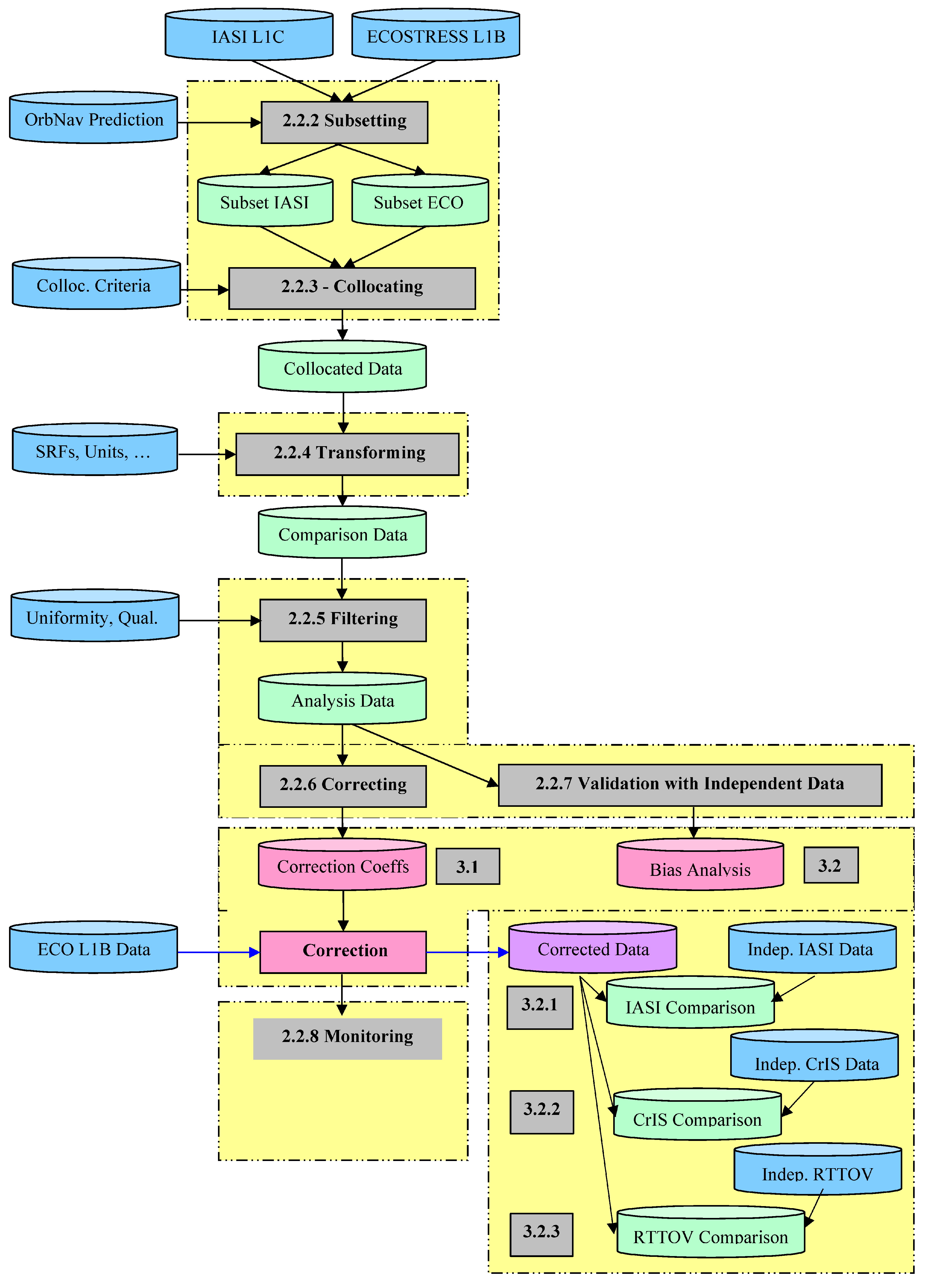
Here, we describe the correction method and its validation with three independent comparison datasets. Figure 1 is a chart of the workflow, modified from [20]. Numbers in the grey boxes refer to section numbers in this paper. Blue ovals represent input data, green ovals represent data undergoing processing, and the purple oval represents the corrected data.

2. Materials and Methods

2.1. Satellite Instruments and Models

2.1.1. ECOSTRESS

ECOSTRESS is a push-whiskbroom filter radiometer on the International Space Station (ISS) with 5 TIR bands (8.29, 8.78, 9.20, 10.49, 12.09 µm) [11,15]. Individual pixels are 69 × 69 m at nadir, there are 128 focal plane pixels in the along-track direction on the focal plane array, and scenes consist of 44 cross-track swaths of 128 × 5400 pixels, so scenes are 5632 × 5400 pixels (along track × cross track) with a scene width of approximately 400 km. Onboard calibration is carried out with two black bodies, which are scanned on every rotation of the scanning mirror. One black body is electrically heated to 325 K, and the other is regulated to approximately 295 K by circulating cooling fluids from the ISS [21,22]. The instrument uses a HgCdTe photoconductive detector array. Because ECOSTRESS is mounted on the ISS, it is on a precessing orbit with an inclination of 51.6°.

2.1.2. Infrared Atmospheric Sounding Interferometer (IASI)

IASI is a Fourier transform spectrometer based on a Michelson interferometer with 8461 channels over the wavelength range of 3.62–15.50 µm. The full-resolution L1C files have 8641 channels with an apodized resolution of 0.5 cm⁻¹, sampled at 0.25 cm⁻¹. IASI is a stop-and-stare instrument. In the cross-track direction, there are 30 steps, and at each step, spectra are acquired in a 2 × 2 array of fields of view (12 km diameter at nadir). IASI instruments have flown on the polar orbiting EUMETSAT Metop A, B and C satellites. Full-resolution operational spectra are available from all 3 IASI instruments. There are 3 bands: the 8.26–15.5 µm band uses HgCdTe photoconductive detectors, the 5.l0–8.26 µm band uses HgCdTe photovoltaic detectors, and the 3.62–5.0 µm band uses InSb photovoltaic detectors [23]. Onboard radiometric calibration of IASI is carried out by measurements of an internal black body at 280 K and a space view on every mirror rotation. Total gaussian uncertainty is less than 0.2 K [24]. IASI has been used operationally by several meteorological agencies as a radiance standard for calibration of polar and geostationary satellite instruments [1,25].

2.1.3. Cross-Track Infrared Sounder (CrIS)

Like IASI, CrIS is a hyperspectral TIR instrument based on a Michelson interferometer. Full-resolution L1B version 3 files have 717 channels, with an apodized spectral resolution of 0.625 cm⁻¹ in the long-wave TIR band (9.14–15.38 µm). The CrIS spectral range allows comparison only with the 10.49 and 12.09 µm ECOSTRESS bands. Like IASI, it is a stop-and-stare instrument. In the cross-track direction, there are 30 earth-view steps, and at each step, spectra are acquired in a 3 × 3 array of fields of view (14 km diameter at nadir). CrIS instruments currently fly on the polar orbiting NOAA SNPP, N-20, and N-21 satellites. Full-resolution operational spectra are available for the instruments on SNPP and N-20. Onboard radiometric calibration uses a space view and an internal black body at 280 K. HgCdTe photovoltaic detectors are used in all wavelength bands [26]. Total gaussian 3-sigma uncertainty is less than 0.3 K in the long-wave infrared band [26]. CrIS has been used operationally by several meteorological agencies as a radiance standard for the calibration of polar and geostationary satellite instruments.

2.1.4. RTTOV Radiative Transfer Model

RTTOV is a radiative transfer model that is used operationally by EUMETSAT and other meteorological agencies. We use RTTOV for independent validation of the ECOSTRESS corrections. Spectral response functions for many TIR instruments including ECOSTRESS are included. Radiative transfer simulations were carried out with RTTOV 12.3 [27] using best-quality NOAA in situ iQuam observations [28] as the surface temperatures, and European Centre for Medium Range Weather Forecasting ERA-5 hourly meteorological reanalysis data at 0.25° spatial scale [29]. Meteorological data (vertical profiles of air temperature and specific humidity, 2 m air temperature and specific humidity, and 10 m wind speed) were bilinearly interpolated in space to in situ NOAA iQuam coordinates and linearly interpolated in time to the ECOSTRESS acquisition time. The Jacobian (K model) was used to calculate at-sensor brightness temperatures, atmospheric absorption and sea surface emissivity, using RTTOV coefficient files for ECOSTRESS. The sea surface emissivity model (IREMIS) includes the influences of the 10 m wind speed, satellite view angle and in situ surface temperature [30]. There were no ECOSTRESS scenes in common between the IASI observations and the RTTOV simulations, confirming the strict spatio-temporal independence of the RTTOV simulations used for validation of the ECOSTRESS corrections.

2.2. Algorithms

The general approach for radiance correction is for the monitored instrument (ECOSTRESS) and the reference instrument (IASI) to make measurements of the same location from the same view angle at the same time, thereby having the same atmospheric path and same surface conditions. In such conditions, the radiances acquired by the two instruments should be the same. In reality, collocations are rarely at exactly the same time with exactly the same viewing angle, especially because the ECOSTRESS instrument is on an orbit with a 51.6° inclination, and IASI on Metop-A, B, and C are on sun-synchronous polar orbits with a 98.7° inclination. Collocations should in principle cover the range of scene radiances encountered by the monitored instrument.

Ideally, the reference instrument should be traceable by an unbroken chain of inter-comparisons with known uncertainties, to a common reference based on a standard like the International System of Units (SI). The traceability chain for IASI was broken at launch, although flight versions A, B, and C were compared before launch to a large-format reference blackbody with platinum resistance thermometers traceable to SI. After nonlinearity and mirror reflectivity corrections, IASI brightness temperatures were within 0.25 K of the black body at 300 K across the entire spectrum [23,31]. Post-launch comparisons indicated that the 3-sigma uncertainty of IASI calibration over the ECOSTRESS wavelengths is between 0.1 and 0.2 K [24,31]. Because IASI is highly stable based on several comparison methods, and because it was well validated pre- and post-launch, it was chosen as a reference standard for intercalibration products by GSICS [31].

Independent collocations with satellite observations by IASI and CrIS, and independent collocations with RTTOV radiative transfer simulations, were used to validate the IASI results.

2.2.1. Data Characterization and Preprocessing

ECOSTRESS Collection 1 files were downloaded from the NASA Land Processes Distributed Active Archive Center (LPDAAC). IASI files were downloaded from the EUMETSAT Data Store [32] using the EUMETSAT Data Access Client (eumdac) [33]. The file chain_file.txt (Appendix A) was used to request remote processing by the EUMETSAT data tailor [34] to produce the IASIL1C data in the netcdf4_satellite format for download. The netcdf4_satellite files contain the geolocation information, spectra, quality assurance values, and coefficients for converting the raw spectra into standard radiance units.

ECOSTRESS files contain 44 swaths of 128 along-track pixels and 5400 cross-track pixels, yielding scenes of 5400 × 5632 pixels. Acquisition times of each swath, and latitudes, longitudes, view zenith angles and view azimuth angles of each pixel are contained in the L1B_GEO geolocation files. Radiances in each band are contained in the L1B_RAD files.

IASI files contain data from a complete orbit, comprising swaths of 30 scan positions and a 2 × 2 array of fields of view (FOVs) at each scan position. FOVs are circular with ~12 km diameter at nadir and are 39 × 20 km ovals at the edge of each swath [35]. FOV center latitudes, longitudes, view zenith angles, view azimuth angles and acquisition times of each FOV are contained in the ncdf4_satellite format files.

CrIS files contain data from a 6 min acquisition, and are comprised of swaths of 30 scan positions and a 3 × 3 array of FOVs at each scan position. FOVs are circular with 14 km diameter at nadir, and are 48 × 24 km ovals at the edge of each swath. FOV center latitudes and longitudes, FOV perimeter polygons, view zenith angles, view azimuth angles, and acquisition times of each FOV are contained in the ncdf4 data files.

2.2.2. Subsetting

Collocations were predicted with the OrbNav utility for simultaneous nadir overpass (SNO) times [36]. These were confirmed by comparing the ECOSTRESS footprint polygons to the IASI acquisition polygons. ECOSTRESS polygons were obtained from the corners of the ECOSTRESS L1B_GEO longitude and latitude. IASI polygons were obtained via the EUMETSAT API [37], geographically constrained by the points in the ECOSTRESS polygon and by ECOSTRESS time ± 30 min.

Collocations with IASI included homogeneous areas covered by land, water, ice, and clouds. The use of land, water, ice and cloud collocations provided a wider range of radiances and brightness temperatures than would be obtained from land, water or clouds alone. This ensured that the calibration corrections would be applicable to all ECOSTRESS scenes. Collocations were restricted to homogeneous areas where the robust standard deviation of ECOSTRESS brightness temperature was less than 0.5 K (see Section 2.2.5), so areas with patchy clouds, land–water boundaries, or steep temperature gradients were avoided. Validation of IASI results with CrIS collocations and RTTOV radiative transfer models was carried out exclusively over strictly independent homogeneous ocean areas.

2.2.3. Collocating

Concurrency in Acquisition Time

The SNO times obtained from OrbNav (Section 2.2.2) are approximate, so actual acquisition times were obtained from the preliminarily identified ECOSTRES:IASI and ECOSTRESS:CrIS SNO files. For each FOV that intersected the ECOSTRESS scene perimeter polygon, the difference in acquisition times was determined. To avoid large differences in atmospheric composition between the IASI or CrIS and ECOSTRESS observations, we used a threshold of 30 min time difference for inclusion in our analysis:

$$\left|IASI FOV time-ECOSTRESS Swath time\right|<1800 \mathrm{s}$$

This criterion allowed an adequate number of collocations without introducing excessive differences in atmospheric conditions. Thirty minutes also provides a time period that will not introduce differences/errors due to ocean dynamics.

Collocation in Space

For each ECOSTRESS:IASI file pair, the perimeters of all IASI fields of view (FOVs) were calculated using the equations in Section 6 of the IASI Level 2 Product Generation Specification [38]. For each ECOSTRESS:CrIS file pair, the perimeters of the CrIS FOVs were obtained from the FOV polygon variables (lat_bnds, lon_bnds) in the data files. For each FOV, the enclosed ECOSTRESS pixels were identified using the sf library in R [39]. Each FOV contained 10,000–30,000 ECOSTRESS pixels. The arithmetic mean view zenith angle, mean, median, standard deviation and robust standard deviation (median absolute difference) among ECOSTRESS pixel radiances in each wavelength band in each FOV were calculated.

Alignment of Viewing Geometry

Data were filtered to ensure that the ECOSTRESS pixels within each IASI or CrIS FOV had similar viewing conditions. Zenith angle alignment is used to assure a similar path length through the atmosphere. Azimuth angle alignment is required for shortwave IR during daylight data acquisitions, but the minimum wavelength of ECOSTRESS is 8.29 µm, where such alignment is not necessary [20].

The following zenith angle criterion was used, where za_ECOSTRESS is the ECOSTRESS zenith angle and za_Hyperspec is the IASI or CrIS zenith angle.

$$\left|{\displaystyle \frac{cos\left(za\_ECOSTRESS\right)}{cos\left(za\_Hyperspec\right)}}-1\right|<0.01$$

(1)

Equation (1) allows a zenith angle difference of 8.07° at nadir and 1.13° at a 29° view zenith angle.

2.2.4. Transforming

Radiance Unit Conversion

The hyperspectral observations of IASI and CrIS need to be matched spectrally with ECOSTRESS by convolution with the ECOSTRESS band spectral response functions (SRFs). IASI and CrIS radiances are reported in wavenumber units (W m⁻² sr⁻¹ (m⁻¹)⁻¹ for IASI and mW m⁻² sr⁻¹ (cm⁻¹)⁻¹ for CrIS), and ECOSTRESS radiances are reported in wavelength units (W m⁻² sr⁻¹ µm⁻¹) so a unit conversion is necessary.

Wavenumber units were converted to wavelength units following [40,41,42]. The logic is that in-band radiance (W m⁻² sr⁻¹) should be the same regardless of the spectral unit.

Sensor reaching radiance L_S (W m⁻² sr⁻¹) is

$$L_S={{\displaystyle \int }}_{{\lambda }_1}^{{\lambda }_2}L{\varphi }_{\lambda }d\lambda ={{\displaystyle \int }}_{{\nu }_1}^{{\nu }_2}L{\varphi }_{\nu }d\nu$$

(2)

where ${\varphi }_{\lambda }$ and ${\varphi }_{\nu }$ are the spectral response functions for the sensor band in wavelength and wavenumber units. The effective radiance L* reaching the sensor (W m⁻² sr⁻¹ µm⁻¹ or W m⁻² sr⁻¹ (cm⁻¹)⁻¹) is obtained by dividing L_S by the band equivalent width W calculated in either wavelength space or wavenumber space:

$$W_{\lambda }={{\displaystyle \int }}_{{\lambda }_1}^{{\lambda }_2}{\varphi }_{\lambda }d\lambda$$

(3)

$$W_{\nu }={{\displaystyle \int }}_{{\nu }_1}^{{\nu }_2}{\varphi }_{\nu }d\nu$$

(4)

$$L*=L_S/W$$

(5)

To convert effective radiance in wavenumber units (L*_ν) to effective radiance in wavelength units (L*_λ),

$$L{*}_{\lambda }=L{*}_{\nu } {\displaystyle \frac{W_{\nu }}{W_{\lambda }}}$$

(6)

To convert radiance in wavelength units (L*_λ) to radiance in wavenumber units (L*_ν),

$$L{*}_{\nu }=L{*}_{\lambda } {\displaystyle \frac{W_{\lambda }}{W_{\nu }}}$$

(7)

Band-equivalent widths of ECOSTRESS channels are reported in

Table 1. Band-equivalent widths of ECOSTRESS channels in wavenumber units and wavelength units.

Band	8.28 µm	8.78 µm	9.20 µm	10.49 µm	12.09 µm
Wν (cm−1)	53.31839	44.00852	47.94716	38.92971	43.13192
Wλ (µm)	0.3668045	0.3414509	0.4062228	0.42723	0.62900052

. Values were calculated using uninterpolated spectral response functions [43] with sampling intervals of 0.00985 µm.

Conversion of ECOSTRESS Collection 1 Radiances to Collection 2 Radiances

The analysis in this paper was carried out using ECOSTRESS Collection 1 L1B_RAD radiance files. For compatibility with all ECOSTRESS data, ECOSTRESS Collection 2 equivalent radiances were calculated from the Collection 1 radiances by applying

Table 2. Radiance bias correction coefficients used in production of ECOSTRESS Collection 2 [16]. These coefficients were used by JPL to reduce the radiance biases detected in ECOSTRESS Collection 1.

Band	8.28 µm	8.78 µm	9.20 µm	10.49 µm	12.09 µm
Gain	0.8757	0.9429	0.9148	0.9507	0.9448
Offset	0.9680	0.5110	0.6181	0.5208	0.5515

gains and offsets, which are used by the Jet Propulsion Laboratory in operational production of ECOSTRESS Collection 2 radiance files [16].

Spectral Matching

The ECOSTRESS SRFs [43] were linearly interpolated to the IASI or CrIS channel wavenumbers. Although Di et al. [44] recommend spline interpolation of SRFs for intercomparison of broadband instruments with hyperspectral sounders, we encountered instability and therefore used the linear method. The 99th percentile of the resulting BT difference between the two methods is less than 1 mK, except in the 9.02 µm band, where it is less than 3 mK. The IASI and CrIS spectra were convolved with the interpolated ECOSTRESS SRFs to create simulated radiances for comparison with ECOSTRESS acquisitions.

$$L_{Sim\_\nu }={\displaystyle \frac{\int L_{\nu }{\Phi }_{\nu }d\nu }{\int {\Phi }_{\nu }d\nu }}$$

(8)

where L_{Sim_ν} is the simulated ECOSTRESS band radiance in wavenumber space, based on the collocated IASI or CrIS spectrum, L_ν is the IASI or CrIS radiance at wavenumber ν and Φ_ν is the ECOSTRESS band spectral response at wavenumber ν. IASI provides complete spectral coverage of the ECOSTRESS bands, whereas CrIS provides coverage of only the 10.49 and 12.09 µm bands. This simulated radiance is what we termed “effective radiance” in Equation (5).

This calculation takes advantage of the large number of IASI channels convolved to obtain the ECOSTRESS-equivalent radiance. The resolution in wavenumber space of IASI spectra is 0.25 cm⁻¹, so there are between 228 and 360 IASI channels used in the calculation of the ECOSTRESS-equivalent radiance in each field of view (this is the number of channels where the ECOSTRESS spectral response function is greater than 0.05). The large sample size in the convolution reduces IASI random errors below the per-channel radiometric noise (NEdT) of ~0.05 K to the mK range [25].

For direct comparison with ECOSTRESS radiances, the simulated band radiances were converted from wavenumber space to wavelength space (Equation (6)) [40,41], as described in Section 2.2.4 Radiance Units Conversion.

Brightness Temperature Data

Brightness temperatures of the ECOSTRESS pixels were calculated from radiances with a look-up-table provided by the LPDAAC [45]. Brightness temperature of the IASI or CrIS FOV was calculated by first converting the IASI or CrIS radiance from wavenumber space to wavelength space (Section 2.2.4 Radiance Units Conversion), and then applying the lookup-table.

The alternative requires calculating the central wavelength of each ECOSTRESS band [43]:

$$\mathit{I}\mathit{A}\mathit{S}{\mathit{I}}_{\mathit{c}\mathit{w}\mathit{l}}= {\displaystyle \frac{\int \lambda {\Phi }_{\lambda }d\lambda }{\int {\Phi }_{\lambda }d\lambda }}$$

(9)

In wavelength space, the central wavelength and integrated IASI radiance for each band are used in the inverse Planck equation to calculate the brightness temperature (BT):

$$\mathit{B}{\mathit{T}}_{\mathit{I}\mathit{A}\mathit{S}{\mathit{I}}_{\mathit{\lambda }}}= {\displaystyle \frac{{\mathit{c}}_2}{\mathit{\lambda }ln\left(\frac{{\mathit{c}}_1}{1+{\mathit{\lambda }}^5{\mathit{L}}_{\mathit{S}\mathit{i}\mathit{m}▁\mathit{\lambda }}}\right)}}$$

(10)

where λ is the IASI central wavelength, L_{Sim_λ} is the spectrally matched IASI radiance at wavelength λ, c₁ is 1.191042 × 10⁸ W m⁻² sr⁻¹ µm⁻¹ and c₂ is 1.4387752 × 10⁴ K µm.

In wavenumber space, the central wavenumber and integrated IASI radiance for each band are used in the inverse Planck equation to calculate the brightness temperature (BT):

$$\mathit{B}{\mathit{T}}_{\mathit{I}\mathit{A}\mathit{S}{\mathit{I}}_{\mathit{\nu }}}= {\displaystyle \frac{{\mathit{c}}_2\nu }{ln\left(\frac{{\mathit{c}}_1{\mathit{\nu }}^3}{1+{\mathit{L}}_{\mathit{S}\mathit{i}\mathit{m}▁\mathit{\nu }}}\right)}}$$

(11)

where ν is the IASI central wavenumber, L_{Sim_ν} is the spectrally matched IASI radiance at wavenumber ν, c₁ is 1.191042 × 10⁻⁵ mW m⁻² sr⁻¹ (cm⁻¹) ⁻¹ and c₂ is 1.4387752 K cm.

The approximation of polychromatic radiance in an ECOSTRESS band to a central wavelength or wavenumber introduces brightness temperature errors because the distribution of polychromatic radiances within a spectral window changes with temperature. The literature [2,44,46,47] suggests a linear correction of the brightness temperatures predicted by the central wavelength or central wavenumber of the spectral response. Correction coefficients are estimated by regression of channel radiance integrals versus temperature [44]. Correction coefficients for ECOSTRESS channels are included in the RTTOV coefficients files for ECOSTRESS [48]. However, the RTTOV BT correction coefficients are based on the ECOSTRESS spectral response functions [43], adjusted by converting all negative values to zero. The RTTOV correction coefficients will introduce errors if used with the original ECOSTRESS spectral response functions, which include negative values.

2.2.5. Filtering

Spatial uniformity within the FOV is important especially when correction coefficients are derived for individual detectors in the focal plane array, which can be influenced by the spatial patterns of clouds and other features in the FOVs. Here, the robust standard deviation (RSD) of the ECOSTRESS brightness temperatures was used as a measure of uniformity of each FOV.

The robust standard deviation (RSD) of the BT biases was calculated from the median absolute deviation (MAD):

$$\mathit{M}\mathit{A}\mathit{D}=\mathit{m}\mathit{e}\mathit{d}\mathit{i}\mathit{a}\mathit{n}\left(\left|{\mathit{X}}_{\mathit{i}}-\tilde{\mathit{X}}\right|\right)$$

(12)

$$\mathit{R}\mathit{S}\mathit{D}=\mathit{M}\mathit{A}\mathit{D}\times 1.4826$$

(13)

Although some authors have argued that the use of thresholds is suboptimal [1], others have used thresholds to exclude FOVs. For example, Mittaz and co-authors [49] used a threshold of 1 K, while Tobin and co-authors [50,51] used a threshold of 0.2 K.

We rejected FOVs with RSD(BT_10.49µm) > 0.5 K. This removed cases where there were patchy clouds or land–water boundaries in the ECOSTRESS scene.

2.2.6. Correcting

Calculation of Correction Coefficients

The observations of the reference instrument (IASI) and the monitored instrument (ECOSTRESS) are fitted to a linear model. We assume the uncertainty associated with the median x_i of the ECOSTRESS measurements within an IASI FOV is equivalent to their robust standard deviation RSD_i, and that the IASI measurement y_i within the FOV has much lower uncertainty because it is derived by convolving a large number of IASI observations with the spectral response function of the ECOSTRESS wavelength band. We use a weighted regression, using 1/RSD_i as the weight for each ECOSTRESS FOV mean x_i.

Following GSICS recommendations [20], the regression equation

$${\mathit{R}}_{\mathit{E}\mathit{C}\mathit{O}\mathit{S}\mathit{T}\mathit{R}\mathit{E}\mathit{S}\mathit{S}}=\mathit{a}+\mathit{b}\times {\mathit{R}}_{\mathit{I}\mathit{A}\mathit{S}\mathit{I}}$$

(14)

is inverted to convert ECOSTRESS radiances to radiances consistent with the IASI reference instrument ${\widehat{\mathit{R}}}_{\mathit{I}\mathit{A}\mathit{S}\mathit{I}}$

$${\widehat{\mathit{R}}}_{\mathit{I}\mathit{A}\mathit{S}\mathit{I}}=\mathit{O}\mathit{f}\mathit{f}\mathit{s}\mathit{e}\mathit{t}+\mathit{G}\mathit{a}\mathit{i}\mathit{n}\times {\mathit{R}}_{\mathit{E}\mathit{C}\mathit{O}\mathit{S}\mathit{T}\mathit{R}\mathit{E}\mathit{S}\mathit{S}}$$

(15)

where

$$\mathit{O}\mathit{f}\mathit{f}\mathit{s}\mathit{e}\mathit{t}=-{\displaystyle \frac{\mathit{a}}{\mathit{b}}}\mathrm{and}\mathit{G}\mathit{a}\mathit{i}\mathit{n}={\displaystyle \frac{1}{\mathit{b}}}$$

(16)

with uncertainty

$${\mathit{\sigma }}_{{\widehat{\mathit{R}}}_{\mathit{I}\mathit{A}\mathit{S}\mathit{I}}}^2={\left({\displaystyle \frac{{\mathit{\sigma }}_{\mathit{a}}}{\mathit{b}}}\right)}^2+{\left[\left({\mathit{R}}_{\mathit{E}\mathit{C}\mathit{O}\mathit{S}\mathit{T}\mathit{R}\mathit{E}\mathit{S}\mathit{S}}-\mathit{a}\right){\mathit{\sigma }}_{\mathit{b}}\right]}^2-2{\displaystyle \frac{\left({\mathit{R}}_{\mathit{E}\mathit{C}\mathit{O}\mathit{S}\mathit{T}\mathit{R}\mathit{E}\mathit{S}\mathit{S}}-\mathit{a}\right)}{\mathit{b}}}{\mathit{\sigma }}_{\mathit{a}\mathit{b}}$$

(17)

The sigma terms are obtained from the variance–covariance matrix of the regression: σ_a and σ_b, are the square roots of the variances of a and b, and σ_ab is the covariance of a and b.

Temporal Drift of the Corrections

To measure temporal drift, correction coefficients were calculated for each month with at least 50 matchups in the record. The rates of change in the gains and offsets were measured from the slopes of regressions against time, weighted by the standard errors of the monthly coefficients.

Measures of Quality of the Corrections

The bias of the corrected radiance was calculated as

Bias = Corrected Radiance − IASI Radiance

(18)

The median absolute deviation (MAD) was used as a robust measure of the variability around the median bias. The slope of the regression of radiance bias versus IASI radiance, and the slope of the regression of brightness temperature bias versus IASI brightness temperature are both measures of the effectiveness of the correction method. Slopes of zero are the goal, so the absolute values of the slope are inversely related to the quality of the correction.

Additional Sources of Uncertainty

There are multiple additional sources of uncertainty in the estimation of the corrections, including spatial and temporal noise in ECOSTRESS data, non-uniformity of the matchup locations, spatial and temporal mismatch between ECOSTRESS and the reference observations, and radiometric uncertainty in both ECOSTRESS and IASI observations.

ECOSTRESS Geolocation Uncertainty

ECOSTRESS geolocation uncertainty was estimated from 100 coastal scenes in Galicia NW Spain (2022 to 2025). ECOSTRESS Tiled Georeferenced Land Surface Temperature geotiff files (ECOv002_L2T_LSTE) from Harmonized Landsat Sentinel tile 29TNH were analyzed in QGIS software [52], and the geographic error between the coastline and the image was recorded. The standard deviation and RSD of the geographic errors were used as proxies for ECOSTRESS geolocation uncertainty.

Sensitivity of radiometric uncertainty to changes in spatial mismatch between IASI and ECOSTRESS observations was estimated by measuring the change in FOV median BT and radiance after shifting the position of each IASI FOV by 1, 2, 3, 4, 5, and 8 km in both the along-track and the cross-track directions in the matching ECOSTRESS scene. To maintain consistency with the methods of Section 2.2.5, we rejected shifted FOVs with RSD(BT_10.49µm) > 0.5 K. We approximated the sensitivity of radiance or BT to geolocation error (∂R/∂x or ∂T/∂x) as the slope of the regression of FOV radiance or BT bias versus geolocation error magnitude. The regression was calculated from all matchups in 2024. ECOSTRESS radiometric uncertainty due to spatial mismatch was calculated as

u(R_Geolocation) = (∂R/∂x) × median (ECOSTRESS geolocation error)

(19)

u(T_Geolocation) = (∂T/∂x) × median (ECOSTRESS geolocation error)

(20)

Temporal Mismatch Uncertainty

Temporal mismatch uncertainty was estimated from the SD and RSD of the acquisition time differences in the IASI matchup dataset (2018–2024).

Sensitivity of radiometric uncertainty to changes in temporal mismatch between IASI and ECOSTRESS acquisitions was estimated from the regression between acquisition time difference and BT or radiance bias. We approximated the sensitivity of radiance or BT to acquisition time uncertainty (∂R/∂t or ∂T/∂t) with the slope of the regression. The regression was calculated from all matchups in 2024. The ECOSTRESS radiometric uncertainty due to temporal mismatch was calculated as

u(R_{Temporal Mismatch}) = (∂R/∂t) × RSD (temporal mismatch)

(21)

u(T_{Temporal Mismatch}) = (∂T/∂t) × RSD (temporal mismatch)

(22)

IASI and ECOSTRESS Radiometric Uncertainty Due to Spatial and Temporal Noise

IASI radiometric uncertainty of spectral measurements is between 0.05 K and 0.08 K in the wavelength range of ECOSTRESS [24]. Errors arising from the convolution of IASI spectra over ECOSTRESS SRF wavelengths are on the order of 1–2 mK [53]. Convolutions used 2635 IASI channels because ECOSTRESS SRFs cover the range of 769.25 to 1427.75 cm⁻¹.

ECOSTRESS radiometric uncertainty was estimated from the matchup FOVs as RSD(R) or RSD(T). This uncertainty includes spatial and temporal noise and non-uniformity of the matchup locations. This uncertainty propagates through the calibration equation as described in Section 2.2.6 Calculation of Correction Coefficients (Equation (17)).

Uncertainty due to ECOSTRESS temporal noise was estimated from pre-launch NEdT measurements [54]. We used the estimate of 625 mK reported by [14] for uncertainty due to ECOSTRESS spatial noise. The averaging of the ECOSTRESS pixels in the IASI field of view reduces these uncertainties by 1/√N, where N is the number of pixels.

Combined Uncertainty

The combined radiance uncertainty was calculated by

$${\mathit{\sigma }}^2\left(\mathit{R}\right)={{\displaystyle \sum }}_{\mathit{i}=1}^{\mathit{N}}{\left({\displaystyle \frac{\partial \mathit{R}}{\partial \mathit{x}}}\mathit{u}\left({\mathit{x}}_{\mathit{i}}\right)\right)}^2+2{{\displaystyle \sum }}_{\mathit{i}=1}^{\mathit{N}-1}{{\displaystyle \sum }}_{\mathit{j}=\mathit{i}+1}^{\mathit{N}}{\displaystyle \frac{\partial \mathit{R}}{\partial {\mathit{x}}_{\mathit{i}}}}{\displaystyle \frac{\partial \mathit{R}}{\mathit{d}{\mathit{x}}_{\mathit{j}}}}\mathit{u}\left({\mathit{x}}_{\mathit{i}}\right)\mathit{u}\left({\mathit{x}}_{\mathit{j}}\right)\mathit{r}\left({\mathit{x}}_{\mathit{i}}, {\mathit{x}}_{\mathit{j}}\right)$$

(23)

The combined brightness temperature uncertainty replaces R with T in the equation.

The uncertainties of individual measured quantities x_i are u(x_i) and the error correlation between quantities x_i and x_j is r(x_i, x_j). We used the worst case of perfect error correlation between measured quantities r(x_i, x_j) = 1 since the error correlations were unclear.

2.2.7. Validation of the Corrections

The ECOSTRESS:IASI matchup dataset was divided in half, where one half of the ECOSTRESS scenes were used for generating the correction coefficients and the other half of the scenes were used for validation, ensuring strict spatial and temporal independence of calibration and validation data. One hundred replicates of this procedure were performed. The replicate that produced the median value of the 100 gain coefficients was chosen as the best representative of the correction coefficients, and the validation dataset from that replicate was used for the IASI validation.

Corrections were validated in 3 steps by comparison with spatially and temporally disjoint collocations between ECOSTRESS and fully independent IASI and CrIS hyperspectral measurements, and to RTTOV radiative transfer simulations carried out at spatially and temporally disjoint collocations between ECOSTRESS and NOAA iQuam in situ observations. The IASI matchups were over both land and water, whereas the CrIS and RTTOV matchups were exclusively over the ocean. The RTTOV matchups were previously analyzed [14]. The IASI, CrIS and RTTOV analyses had no ECOSTRESS scenes in common with each other or with the data used for generation of the calibration coefficients so they are strictly spatially and temporally disjoint.

Radiance biases were calculated between ECOSTRESS and collocated IASI, CrIS and RTTOV observations. ECOSTRESS and RTTOV radiances are in wavelength units (W m⁻² sr⁻¹ µm⁻¹). Collocated IASI and CrIS hyperspectral radiances were spectrally matched to ECOSTRESS bands by convolution with ECOSTRESS spectral response functions as described in Section 2.2.4 Spectral Matching (Equation (8)), and units were converted from wavenumber units (mW m⁻² sr⁻¹ (cm⁻¹)⁻¹ to wavelength units as described in Section 2.2.4 Radiance Units Conversion (Equation (7)). Brightness temperatures were calculated from the radiances as described in Section 2.2.4 Brightness Temperature Data, and biases were calculated between ECOSTRESS and the collocated IASI, CrIS and RTTOV brightness temperatures as, for example,

$$Bias\left(BT\right)=B{T}_{ECO}-B{T}_{IASI}$$

(24)

Validation criteria were the median bias of the corrected data, and the slope of the relation between bias and temperature. We expected that the corrections would reduce the absolute value of the median bias and reduce the absolute value of the slope of the relation between bias and temperature.

2.2.8. Monitoring

Correction coefficients were generated from monthly subsets of the IASI matchup data from September 2018 to December 2024. Coefficients were generated only if there were at least 50 matchups in the month. This was done to reduce inter-month variation in estimates of the coefficients. Time series of the coefficients were plotted and visually examined for evidence of seasonal patterns. The rates of change of the coefficients were calculated by regression.

3. Results

3.1. Corrections

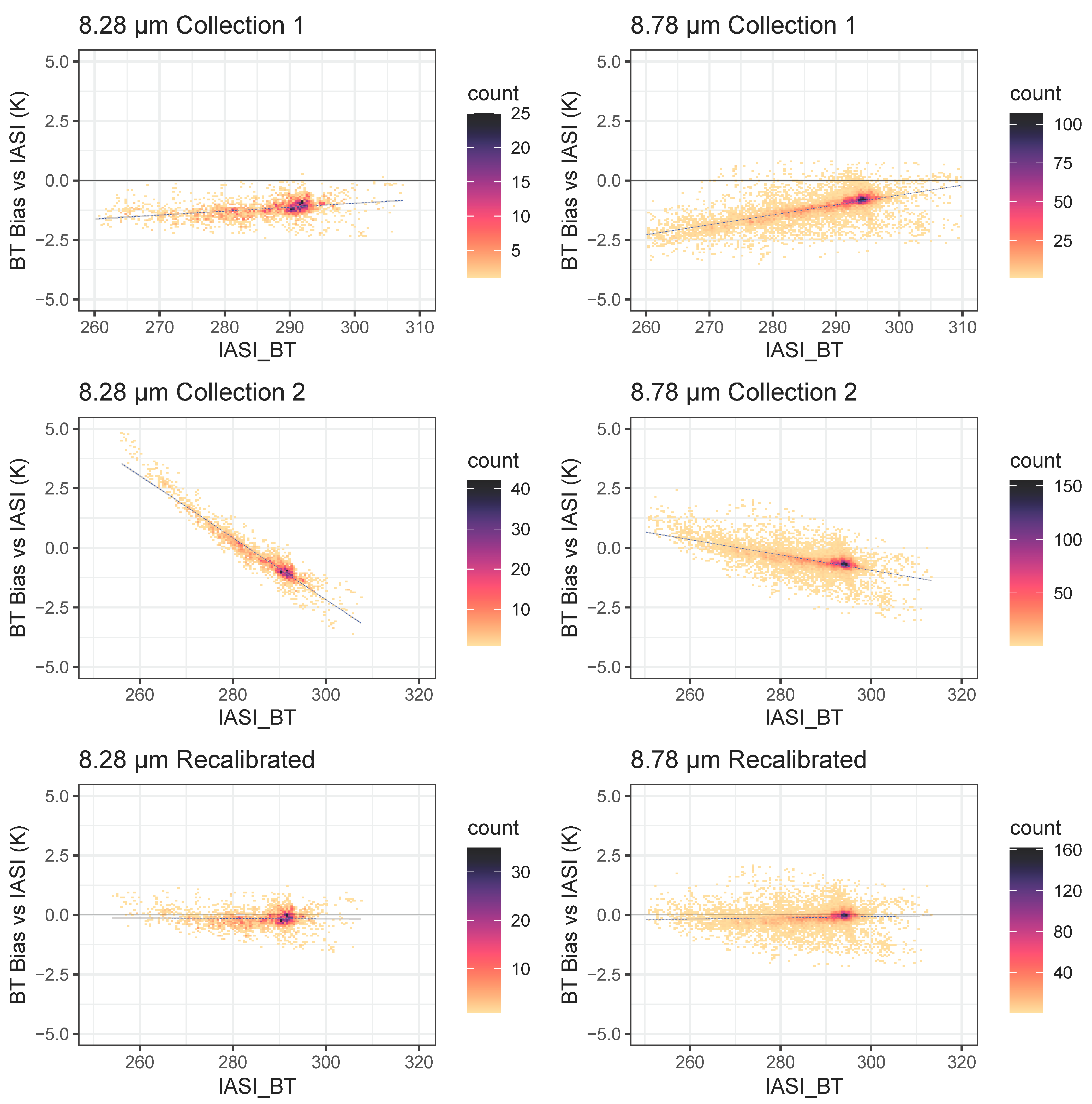
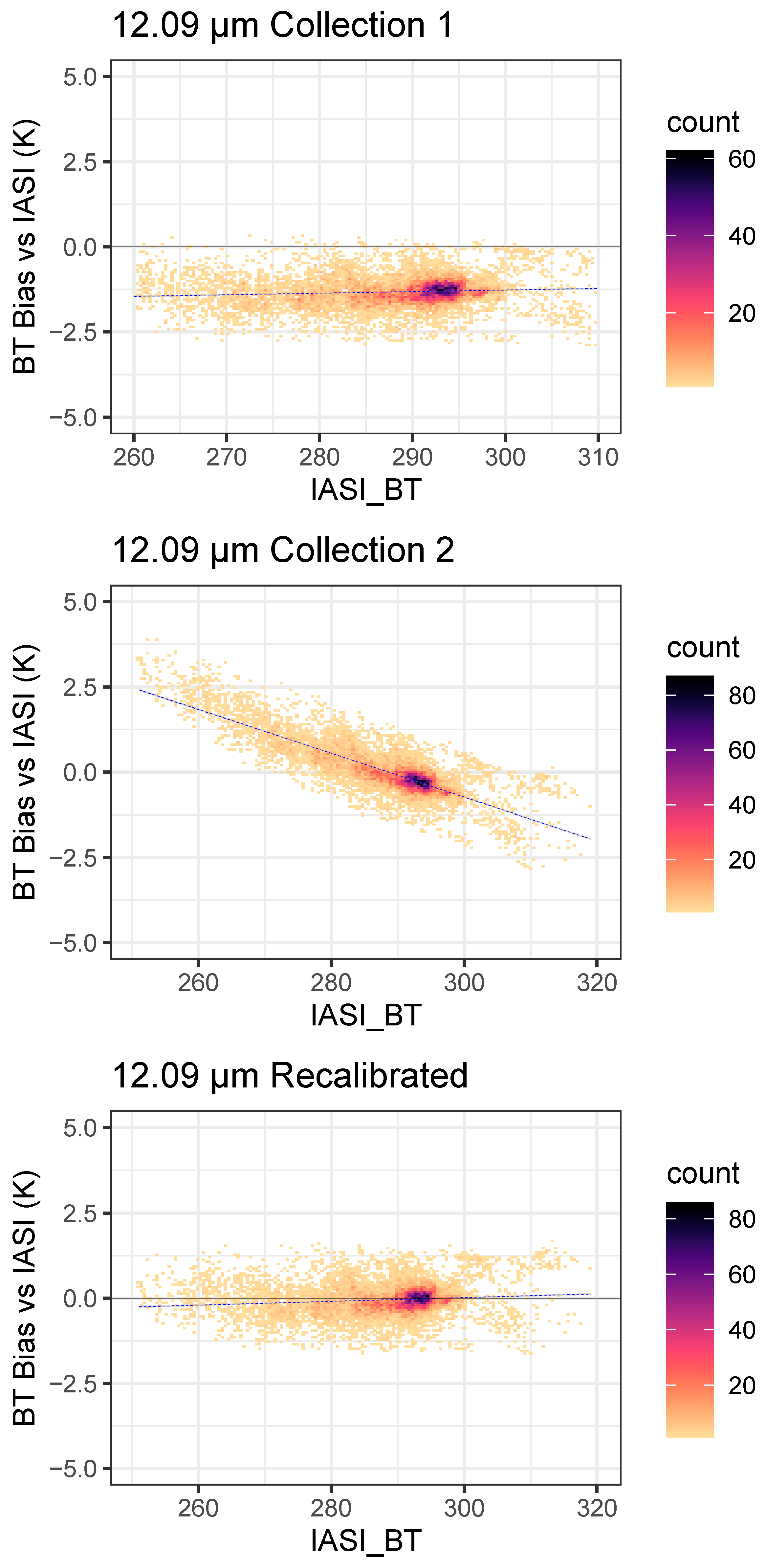
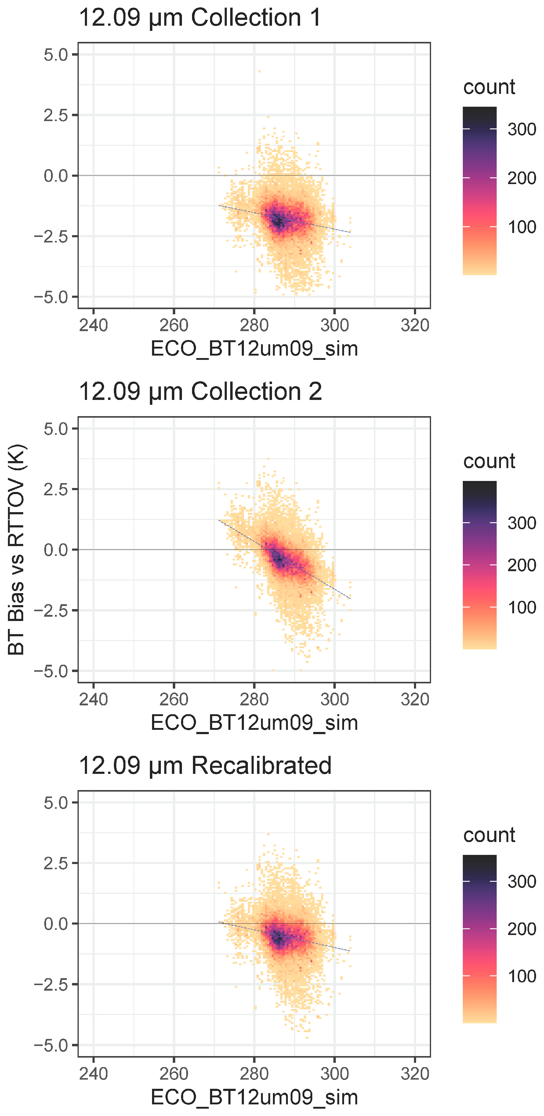
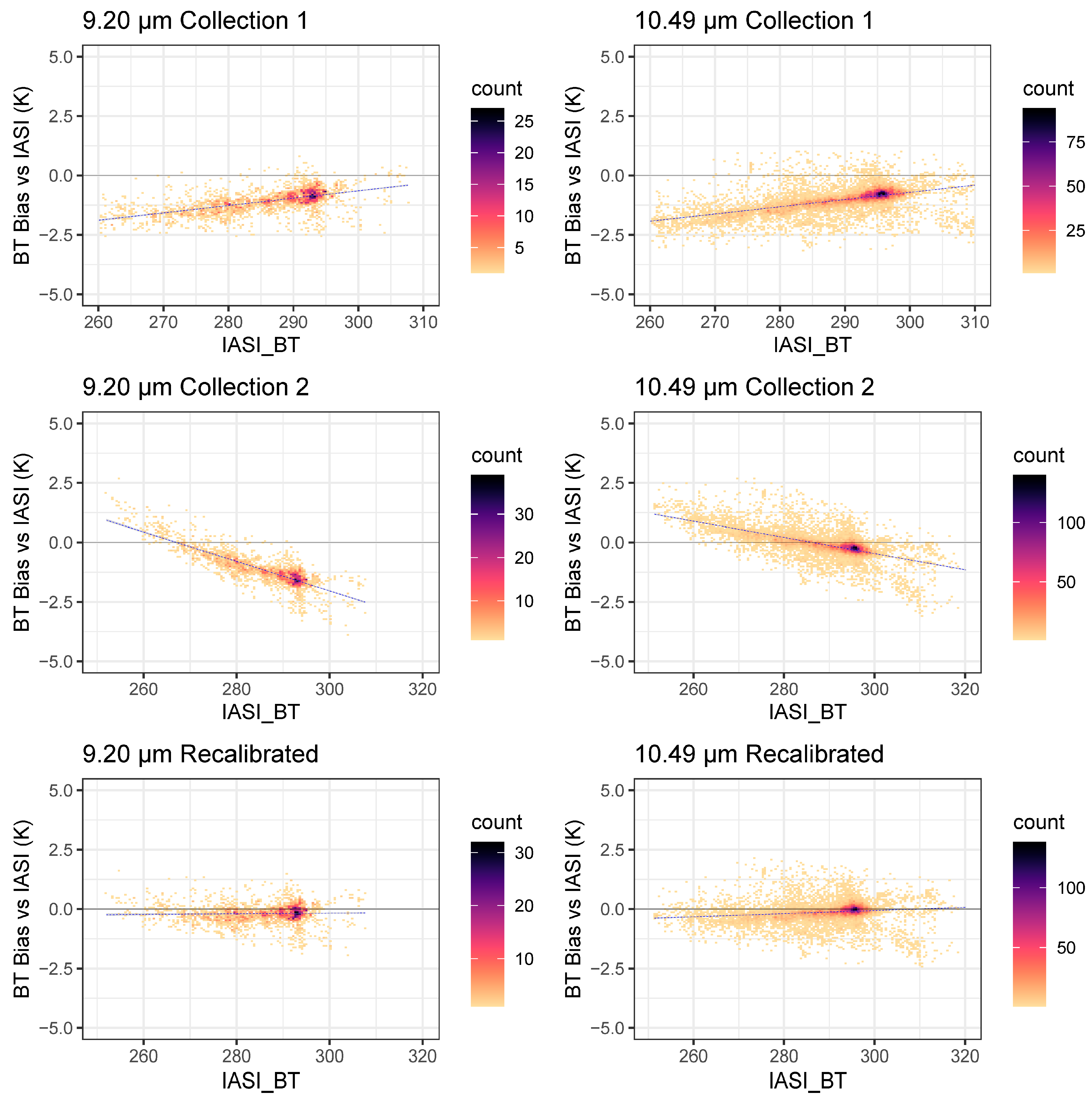
The analysis of the IASI-derived corrections was carried out with a fully independent set of matchups between ECOSTRESS and IASI. There were no ECOSTRESS scenes in common between those used to derive the correction coefficients and those used in the following analysis. ECOSTRESS Collection 1 brightness temperatures were biased cold relative to IASI over most of the temperature range from 240 K to 310 K, and there was a weak positive temperature dependence of the bias (Figure 2, Figure 3 and Figure 4). In contrast, ECOSTRESS − IASI BT biases in ECOSTRESS Collection 2 were nearly zero when averaged across the temperature range, but there were warm biases at low temperatures and cold biases at high temperatures. The changeover point from warm bias to cold bias in Collection 2 differed among the wavelength bands and is probably more related to the slope of the temperature dependence and the median bias of the wavelength band than to a physical mechanism. Collection 2 biases at 250 K were as high as +3.75 K in the 8.28 µm band and +2.5 K in the 9.2 µm band (Figure 2 and Figure 3), and at 310 K, they were as low as −3.75 K in the 8.28, 8.78 and 10.49 µm bands (Figure 2 and Figure 3). The strong negative temperature dependence of the bias in Collection 2 was a major change from the weaker positive temperature dependence in Collection 1 (Figure 2, Figure 3 and Figure 4). The temperature dependence of the bias is probably caused by nonlinearities in the HgCdTe detectors [55].

The IASI-derived corrections reduced the biases to near zero and reduced the temperature dependence of the biases to near zero (Figure 2, Figure 3 and Figure 4).

The radiance bias correction coefficients derived from the IASI matchups (

Table 3. Radiance bias correction coefficients for ECOSTRESS Collection 1, derived from IASI matchups.

Band	8.28 µm	8.78 µm	9.20 µm	10.49 µm	12.09 µm
Gain	1.0009	0.9797	0.9849	0.9879	1.0114
Offset	0.1455	0.3036	0.2391	0.2187	0.0539
σa	0.0049	0.0031	0.0057	0.0033	0.0029
σb	0.0007	0.0004	0.0007	0.0004	0.0004
σab	−3.2824 × 10−6	−1.2237 × 10−6	−4.1121 × 10−6	−1.3270 × 10−6	−1.1370 × 10−6
R2	0.998	0.998	0.998	0.998	0.998
RMSE	0.048	0.058	0.056	0.059	0.051
N	3406	12,988	3445	13012	12,748

and

Table 4. Radiance bias correction coefficients for ECOSTRESS Collection 2, derived from IASI matchups.

Band	8.28 µm	8.78 µm	9.20 µm	10.49 µm	12.09 µm
Gain	1.1430	1.0390	1.0767	1.0391	1.0705
Offset	−0.9609	−0.2273	−0.4264	−0.3224	−0.5365
σa	0.0043	0.0029	0.0052	0.0032	0.0028
σb	0.0006	0.0004	0.0007	0.0004	0.0004
σab	−2.5171 × 10−6	−1.0879 × 10−6	−3.4412 × 10−6	−1.1994 × 10−6	−1.0149 × 10−6
R2	0.998	0.998	0.998	0.998	0.998
RMSE	0.045	0.056	0.053	0.058	0.0500
N	3406	12,988	3445	13,012	12,748

) were calculated using Equation (16). The variances associated with the regression (σ_a, σ_b, σ_ab) are used with Equation (17) to calculate uncertainties of the correction process. All correction regressions had R² > 0.99, which provides high confidence in the results.

At 300 K, uncertainties of the corrections were between 0.019 and 0.037 K for recalibration of both Collection 1 and Collection 2 (

Table 5. Uncertainty (K) of recalibration as a function of scene temperature in ECOSTRESS Collections 1 and 2.

Collection	Temperature (K)	8.28 µm	8.78 µm	9.20 µm	10.49 µm	12.09 µm
1	240	0.0410	0.0227	0.0438	0.0260	0.0410
1	300	0.0318	0.0188	0.0367	0.0233	0.0318
1	360	0.0282	0.0172	0.0341	0.0226	0.0282
2	240	0.0467	0.0246	0.0471	0.0276	0.0467
2	300	0.0313	0.0188	0.0363	0.0233	0.0313
2	360	0.0269	0.0169	0.0331	0.0223	0.0269

). The largest uncertainties were for calibration of the 8.28 and 9.20 µm bands—the two bands that were not available between 15 May 2019 and 17 May 2023 and thus had fewer observations (Table 3 and Table 4).

3.2. Validation of Scene-Level Corrections

3.2.1. Comparisons with Independent IASI Collocations over Land and Water

This comparison was carried out with a strictly independent set of matchups between IASI and ECOSTRESS. There were no ECOSTRESS scenes in common between those used to generate the correction coefficients and those used in this comparison. Corrections derived from the IASI matchups reduced the median radiance bias in the 8.28, 8.78 and 9.20 µm bands by approximately one order of magnitude to between 5 and 9 mW m⁻² sr⁻¹ µm⁻¹ (

Table 6. ECOSTRESS − IASI radiance biases (W m⁻² sr⁻¹ µm⁻¹) in ECOSTRESS Collections 1 and 2, and after correction. Radiance dependence of the radiance biases (rows 4–6 in table) is unitless.

Band	8.28 µm	8.78 µm	9.20 µm	10.49 µm	12.09 µm
Median Rad Bias Collection 1	−0.160	−0.141	−0.133	−0.113	−0.140
Median Rad Bias Collection 2 (JPL correction)	−0.0980	−0.074	−0.178	−0.004	−0.010
Median Rad Bias Corrected (IASI correction)	−0.008	0.005	−0.008	0.004	−0.002
Rad Dep Bias Collection 1	0.0011	0.0245	0.0176	0.0174	−0.0041
Rad Dep Bias Collection 2 (JPL correction)	−0.1407	−0.0348	−0.0740	−0.0336	−0.0628
Rad Dep Bias Corrected (IASI correction)	0.0019	0.0040	0.0025	0.0053	0.0072
N	3364	12,693	3386	12,764	12,528

). In the 10.49 and 12.09 µm bands, the correction reduced the Collection 1 bias by one order of magnitude and had a much smaller effect on the ECOSTRESS Collection 2 bias (Table 6). The radiance dependence of the Collection 1 bias was changed very little in the 8.28 and 12.09 µm bands, but was reduced by a factor of three to eight in the other bands (Table 6). Collection 2 bias was reduced by one to two orders of magnitude. Overall, the IASI correction provides a big improvement over Collections 1 and 2.

IASI corrections reduced the median BT bias to between −0.181 and −0.053 K, which is an order of magnitude improvement in most cases (

Table 7. ECOSTRESS − IASI brightness temperature biases (K) in ECOSTRESS Collections 1 and 2, and after correction. Temperature dependence of the brightness temperature biases (rows 4–6 in table) is unitless.

Band	8.28 µm	8.78 µm	9.20 µm	10.49 µm	12.09 µm
Median BT Bias Collection 1	−1.183	−1.019	−1.023	−0.947	−1.325
Median BT Bias Collection 2 (JPL correction)	−0.732	−0.590	−1.298	−0.158	−0.134
Median BT Bias Corrected (IASI correction)	−0.161	−0.083	−0.181	−0.106	−0.053
Temp Dep Bias Collection 1	0.0161	0.0413	0.0307	0.0308	0.0067
Temp Dep Bias Collection 2 (JPL correction)	−0.1478	−0.0315	−0.0641	−0.0333	−0.0665
Temp Dep Bias Corrected (IASI correction)	−0.0019	0.0004	0.0001	0.0034	0.0006
N	3364	12,693	3386	12,764	12,528

). The temperature dependence of the BT bias was reduced by the correction to between one and two orders of magnitude to between −0.0019 and +0.0034 (Table 7). The IASI corrections represent a substantial improvement over the corrections performed by JPL in the production of ECOSTRESS Collection 2.

3.2.2. Comparisons with Independent CrIS Collocations over the Ocean

Here, we perform additional validation of the IASI-derived correction using strictly independent CrIS data. There were no ECOSTRESS scenes in common between those used to generate the correction coefficients and those used in this comparison, or those used in the IASI comparison. CrIS provides radiance data for a fully independent test of the quality of the corrections because the data come from a completely different kind of hyperspectral instrument and from strictly disjoint collocations in space and time, but have the potential issue that CrIS radiances are 0.1 to 0.2 K cold-biased relative to IASI radiances [56].

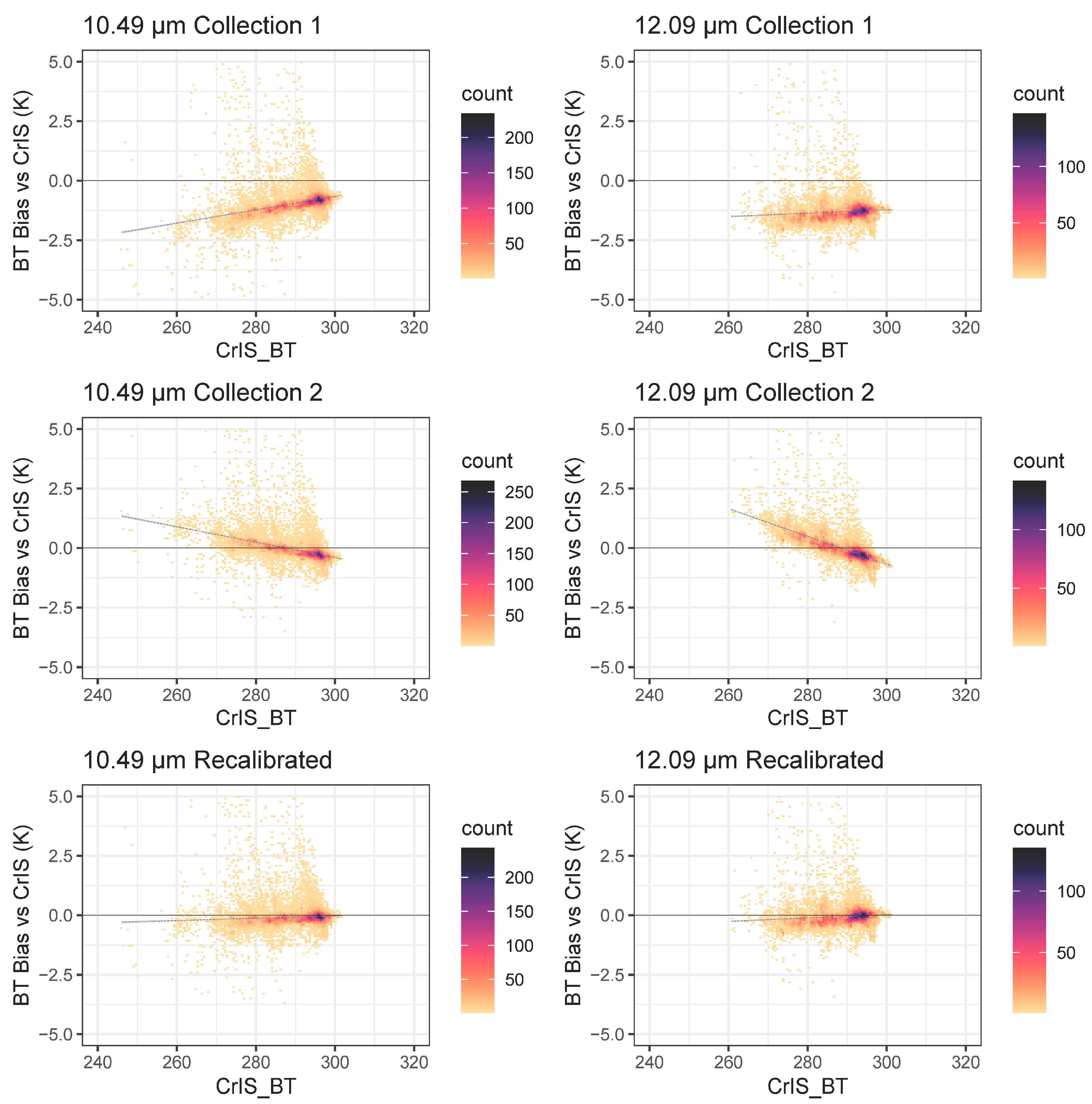
ECOSTRESS Collection 1 median radiances were biased low relative to CrIS by between 0.167 and 0.195 W m⁻² sr⁻¹ µm⁻¹ in the 10.49 and 12.09 µm bands (

Table 8. ECOSTRESS − CrIS radiance biases (W m⁻² sr⁻¹ µm⁻¹) in ECOSTRESS Collections 1 and 2, and after the IASI-derived correction. Radiance dependence of the radiance biases (rows 4–6 in table) is unitless.

Band	10.49 µm	12.09 µm
Median Radiance Bias Collection 1	−0.195	−0.167
Median Radiance Bias Collection 2 (JPL correction)	−0.095	−0.043
Median Radiance Bias Corrected (IASI correction)	−0.086	−0.028
Rad Dependence Bias Collection 1	0.0069	0.0303
Rad Dependence Bias Collection 2 (JPL correction)	−0.1183	−0.0285
Rad Dependence Bias Corrected (IASI correction)	−0.0224	−0.0189
N	7725	7188

), and brightness temperatures were biased cold by between 0.932 and 1.328 K in the 10.49 and 12.09 µm bands respectively (Figure 5,

Table 9. ECOSTRESS − CrIS brightness temperature biases (K) in ECOSTRESS Collections 1 and 2 and after the IASI-derived correction. Temperature dependence of the BT biases (rows 4–6 in table) is unitless.

Band	10.49 µm	12.09 µm
Median BT Bias Collection 1	−0.968	−1.348
Median BT Bias Collection 2 (JPL correction)	−0.142	−0.1128
Median BT Bias Corrected (IASI correction)	−0.120	−0.088
Temp Dependence Bias Collection 1	0.0280	0.0070
Temp Dependence Bias Collection 2 (JPL correction)	−0.0345	−0.0604
Temp Dependence Bias Corrected (IASI correction)	0.0035	0.0055
N	7726	7188

).

Median ECOSTRESS − CrIS biases in Collection 1 were reduced by the corrections JPL used to produce Collection 2 (Table 8 and Table 9), but the temperature dependence of the biases was increased in Collection 2 (Figure 5, Table 8 and Table 9). The corrections derived from the IASI matchups reduced the median ECOSTRESS − CrIS biases and also reduced the temperature dependence of the biases relative to Collection 1 and relative to the JPL corrections in Collection 2 (Figure 5, Table 8 and Table 9). These results are consistent with the comparisons of corrections with independent IASI collocations (Figure 2, Figure 3 and Figure 4, Table 6 and Table 7).

3.2.3. Comparisons with Independent RTTOV Simulations at Triple Matchups Among ECOSTRESS, In Situ Ocean Observations and Cloud-Free Geostationary Observations

Here, we perform a third validation, with fully independent triple collocations [14] among ECOSTRESS, in situ ocean observations from the NOAA in situ SST Quality Monitor [28,57], cloud-free geostationary satellite observations from NOAA, EUMETSAT and JAXA instruments (ABI, SEVIRI, AHI), and radiative transfer simulations with RTTOV [27]. In the RTTOV simulations, the in situ data were used to constrain skin temperature, and ERA-5 reanalysis data [50] were used for the atmospheric variables. Median ECOSTRESS radiances (observed, simulated) in 3 × 3 pixel regions centered on the in situ and cloud-free geostationary observations were converted to brightness temperatures using the lookup tables provided by the LPDAAC [45]. These analyses were performed on matchups between 10 January 2019 and 30 October 2022. During most of this time ECOSTRESS was only acquiring data from the 8.78, 10.49 and 12.09 µm bands so we restricted the RTTOV analysis to those three bands.

ECOSTRESS radiances were biased low relative to RTTOV radiative transfer simulations in all collections and all three bands (

Table 10. ECOSTRESS − RTTOV Radiance biases (W m⁻² sr⁻¹ µm⁻¹) relative to RTTOV in ECOSTRESS Collections 1 and 2, and after correction. Radiance dependence of the radiance biases is unitless (rows 4–6 in table).

Band	8.78 µm	10.49 µm	12.09 µm
Median Radiance Bias Collection 1	−0.248	−0.188	−0.194
Median Radiance Bias Collection 2 (JPL correction)	−0.153	−0.057	−0.046
Median Radiance Bias Corrected (IASI correction)	−0.094	−0.066	−0.057
Rad Dependence Bias Collection 1	−0.00127	−0.01426	−0.04676
Rad Dependence Bias Collection 2 (JPL correction)	−0.05829	−0.06286	−0.09938
Rad Dependence Bias Corrected (IASI correction)	−0.02261	−0.02783	−0.03827
N	80,072	80,089	80,051

). The biases were smallest after the IASI-derived correction, which also reduced the radiance dependence of the bias relative to Collection 2.

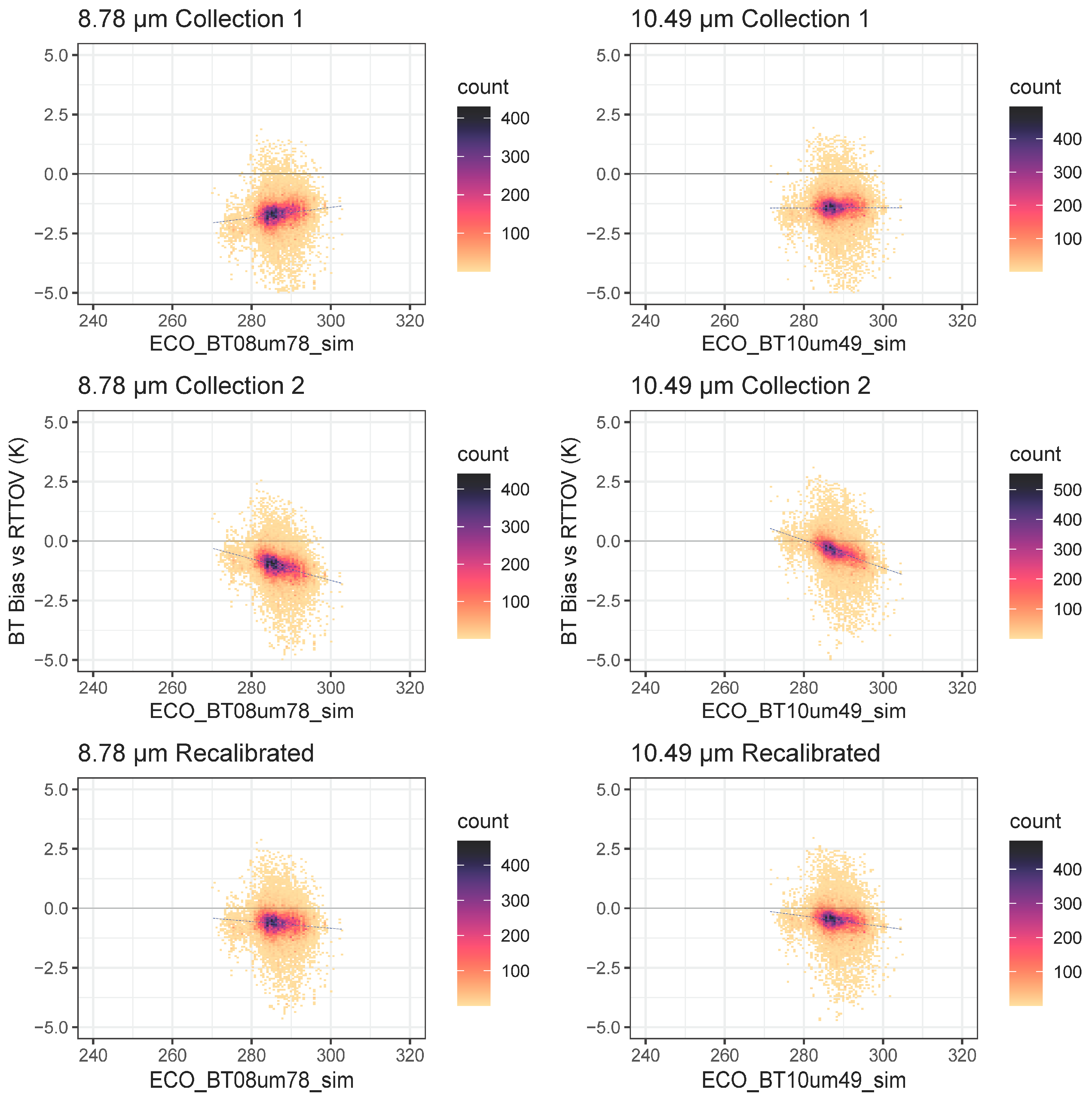
ECOSTRESS Collection 1 brightness temperatures were biased cold by at least 1.4 K relative to RTTOV radiative transfer simulations in all three bands (Figure 6 and Figure 7,

Table 11. ECOSTRESS − RTTOV brightness temperature biases (K) relative to RTTOV in Collection 1, Collection 2, and after correction. Temperature dependence of the brightness temperature biases is unitless (rows 4–6 in table).

Band	8.78 µm	10.49 µm	12.09 µm
Median BT Bias Collection 1	−1.671	−1.406	−1.784
Median BT Bias Collection 2 (JPL correction)	−1.031	−0.426	−0.418
Median BT Bias Corrected (IASI correction)	−0.631	−0.490	−0.524
Temp Dependence Bias Collection 1	0.0218	0.0004	−0.0339
Temp Dependence Bias Collection 2 (JPL correction)	−0.0448	−0.0583	−0.0974
Temp Dependence Bias Corrected (IASI correction)	−0.0138	−0.0224	−0.0351
N	80,072	80,089	80,051

). The corrections applied by JPL in ECOSTRESS Collection 2 reduced the ECOSTRESS − RTTOV biases, but increased the temperature dependence of the biases. The IASI-derived corrections reduced the biases relative to both Collections 1 and 2 and introduced less temperature dependence of the biases than the JPL corrections introduced in Collection 2 (Figure 6 and Figure 7, Table 10 and Table 11).

These results are consistent with the comparisons of corrections within IASI collocations and the comparisons between the corrections and the CrIS collocations (Figure 2, Figure 3, Figure 4 and Figure 5, Table 7 and Table 9). These results confirm that the IASI-derived corrections are an improvement over previous processing of ECOSTRESS radiances in Collections 1 and 2.

3.3. Uncertainties Associated with the Corrections

ECOSTRESS geolocation errors, measured from 100 coastal scenes in NW Spain, ranged from 0.070 km (1 pixel) to 7.360 km (105 pixels), with a median of 0.2 km and an RSD of 1.0 km. The sensitivities of ECOSTRESS radiance and BT uncertainty to spatial mismatch due to ECOSTRESS geolocation errors were on the order of 10⁻³ per km in both the along-track and cross-track directions (

Table 12. Sensitivity of ECOSTRESS radiance and BT uncertainty to spatial mismatch between ECOSTRESS and IASI (W m⁻² sr⁻¹ µm⁻¹ km⁻¹ and K km⁻¹). Values in bold type are significantly different from zero.

Band	Collection	8.28 µm	8.78 µm	9.02 µm	10.49 µm	12.09 µm
Cross track ∂R/∂x	1	1.497 × 10−3	1.571 × 10−3	1.446 × 10−3	1.367 × 10−3	1.247 × 10−3
Along track ∂R/∂x	1	1.264 × 10−3	1.250 × 10−3	1.212 × 10−3	1.122 × 10−3	1.103 × 10−3
Cross track ∂T/∂x	1	1.060 × 10−2	1.069 × 10−2	1.032 × 10−2	1.027 × 10−2	1.156 × 10−2
Along track ∂T/∂x	1	8.773 × 10−3	8.557 × 10−3	8.630 × 10−3	8.393 × 10−3	1.028 × 10−2
Cross track ∂R/∂x	2	1.311 × 10−3	1.482 × 10−3	1.323 × 10−3	1.300 × 10−3	1.179 × 10−3
Along track ∂R/∂x	2	1.107 × 10−3	1.179 × 10−3	1.108 × 10−3	1.067 × 10−3	1.042 × 10−3
Cross track ∂T/∂x	2	9.109 × 10−3	9.967 × 10−3	9.440 × 10−3	7.886 × 10−3	1.080 × 10−2
Along track ∂T/∂x	2	7.553 × 10−3	7.984 × 10−3	7.887 × 10−3	9.678 × 10−3	9.605 × 10−3

). The ECOSTRESS Collection 1 sensitivity to geolocation error is approximately 10% greater than Collection 2 sensitivity, which does not change the order of magnitude effect on uncertainty. Given a median ECOSTRESS geolocation error of 0.2 km, this translates into a systematic radiance uncertainty on the order of 0.2 × 10⁻³ W m⁻² sr⁻¹ µm⁻¹, and a BT uncertainty on the order of less than 1 mK.

Temporal mismatches between IASI and ECOSTRESS ranged from 0 to 30 min, with a median of 13 min and RSD of 8 min. Sensitivities of ECOSTRESS radiance uncertainty to systematic errors in temporal mismatch range from to −1.4 × 10⁻⁵ to +4.3 × 10⁻⁵ W m⁻² sr⁻¹ µm⁻¹ min⁻¹ and sensitivities of brightness temperature uncertainty to systematic errors in temporal mismatch range from −1.4 × 10⁻⁴ to +1.6 × 10⁻⁴ K min⁻¹ (

Table 13. Sensitivity of ECOSTRESS radiance and BT uncertainty to temporal mismatch between ECOSTRESS and IASI (W m⁻² sr⁻¹ µm⁻¹ min⁻¹ and K min⁻¹). Values in bold type are significantly different from zero.

	Collection	8.28 µm	8.78 µm	9.02 µm	10.49 µm	12.09 µm
∂R/∂t	1	−4.702 × 10−6	−1.394 × 10−5	−1.054 × 10−5	−1.143 × 10−5	−7.605 × 10−6
∂T/∂t	1	−7.276 × 10−5	−1.426 × 10−4	−1.163 × 10−4	−1.220 × 10−4	−9.968 × 10−5
∂R/∂t	2	4.325 × 10−5	1.083 × 10−5	2.434 × 10−5	9.614 × 10−6	1.045 × 10−5
∂T/∂t	2	3.218 × 10−4	6.985 × 10−5	1.554 × 10−4	7.561 × 10−5	1.056 × 10−4

).

The systematic radiance bias due to temporal mismatch ranges therefore between 1.8 × 10⁻⁴ and +5.6 × 10⁻⁴ W m⁻² sr⁻¹ µm⁻¹ (13 × −1.4 × 10⁻⁵ to 13 × 4.3 × 10⁻⁵, respectively). The systematic BT bias due temporal mismatch ranges from -1.8 mK to +2.1 mK (13 × −1.4 × 10⁻⁴ to 13 × 1.6 × 10⁻⁴, respectively) depending on the band. The uncertainty due to the variation in temporal mismatch is 0.61 times the above values, or a BT uncertainty ranging from −1.1 mK to +1.3 mK.

There is variation in radiance and BT within the IASI matchup FOVs, which also contributes to uncertainty (

Table 14. Median RSD of ECOSTRESS radiance and BT within IASI matchup FOVs.

	8.28 µm	8.78 µm	9.02 µm	10.49 µm	12.09 µm
RSD(FOV radiance)	0.053	0.033	0.031	0.026	0.043
RSD(FOV BT)	0.357	0.230	0.214	0.198	0.403

). This variation is due to the combined effects of spatial and temporal detector noise, and non-uniformity of the FOVs. These values are constrained by our filtering constraint that FOVs were included in the analysis only if the RSD of BT in the 10.49 µm band was less than 0.5 K.

BT variation within IASI matchup FOVs was on the order of 200 mK in the 8.78, 9.02 and 10.49 µm bands (Table 14). The 12.09 µm band was approximately twice as variable. Radiance variation among bands showed a similar pattern. The uncertainty of the median radiance or BT is the standard error (RSD × 1/√N), where N is the number of FOV pixels.

Total uncertainty of the matchup procedure was roughly estimated using Equation (23). The matchup uncertainty includes effects of spatial and temporal mismatch, along with non-uniformity in the matchup FOVs, which includes spatial and temporal detector noise and non-uniformity of the Earth FOVs themselves (patchy clouds, land–water boundaries, surface temperature gradients) (Equation (25)). The typical number of pixels per FOV (N) = 3 × 10⁴.

$${\left({\mathit{u}}_{\mathit{m}\mathit{a}\mathit{t}\mathit{c}\mathit{h}\mathit{u}\mathit{p}}\right)}^2={\left({\displaystyle \frac{\partial \mathit{B}\mathit{T}}{\partial \mathit{t}}}\mathit{R}\mathit{S}\mathit{D}\left(\mathit{t}\right)\right)}^2+{\left({\displaystyle \frac{\partial \mathit{B}\mathit{T}}{\partial \mathit{x}}}\mathit{R}\mathit{S}\mathit{D}\left(\mathit{x}\right)\right)}^2+{\left({\displaystyle \frac{1}{\sqrt{\mathit{N}}}}\mathit{R}\mathit{S}\mathit{D}\left({\mathit{R}}_{\mathit{F}\mathit{O}\mathit{V}}\right)\right)}^2$$

(25)

The matchup uncertainty per band, based on data in Table 12, Table 13 and Table 14, is shown in

Table 15. Matchup uncertainty of ECOSTRESS BT in IASI or CrIS FOV.

Band	u2 (K2) Assuming No Correlation Between Spatial and Temporal Uncertainty	u (K)
8.28 µm	(−7.3 × 10−5 K/min × 13 min)2 + (8 × 10−3 K/km × 0.2 km)2 + (1/√(3 × 104) × 0.36 K)2	0.0028
8.78 µm	(−1.4 × 10−4 K/min × 13 min)2 + (8 × 10−3 K/km × 0.2 km)2 + (1/√(3 × 104) × 0.23 K)2	0.0028
9.02 µm	(−1.2 × 10−4 K/min × 13 min)2 + (8 × 10−3 K/km × 0.2 km)2 + (1/√(3 × 104) × 0.21 K)2	0.0025
10.49 µm	(−1.2 × 10−4 K/min × 13 min)2 + (8 × 10−3 K/km × 0.2 km)2 + (1/√(3 × 104) × 0.20 K)2	0.0025
12.09 µm	(−1 × 10−4 K/min × 13 min)2 + (1 × 10−2 K/km × 0.2 km)2 + (1/√(3 × 104) × 0.40 K)2	0.0031
	u2 (K2) Assuming Correlation = 1 Between Spatial and Temporal Uncertainty
8.28 µm	(0.0028)2 + 2 × ((−7.3 × 10−5 K/min × 13 min) × (8 × 10−3 K/km × 0.2 km)) × 1	0.0033
8.78 µm	(0.0028) 2 + 2 × ((−1.4 × 10−4 K/min × 13 min) × (8 × 10−3 K/km × 0.2 km)) × 1	0.0037
9.02 µm	(0.0025) 2 + 2 × ((−1.2 × 10−4 K/min × 13 min) × (8 × 10−3 K/km × 0.2 km)) × 1	0.0036
10.49 µm	(0.0025) 2 + 2 × ((−1.2 × 10−4 K/min × 13 min) × (8 × 10−3 K/km × 0.2 km)) × 1	0.0036
12.09 µm	(0.0031) 2 + 2 × ((−1 × 10−4 K/min × 13 min) × (1 × 10−2 K/km × 0.2 km)) × 1	0.0035

. The radiance uncertainties associated with the Collection 1 matchups to IASI or CrIS is between 2.5 and 3.1 mK if we assume no correlation between spatial and temporal uncertainties (Table 15). These uncertainties increase by approximately 0.4 mK if the correlation between the spatial and temporal uncertainties is 1.0.

If we combine the matchup uncertainties (Table 15) with the correction uncertainties (Table 5) to estimate to effect of matchup uncertainty on corrections, we need to include the sensitivity of the correction prediction to matchup uncertainty ∂T_correction/∂T_matchup (Equation (26)). The sensitivity was estimated from the change in corrected BT (ΔBT_corrected) resulting from a 1 mK change in uncorrected BT (ΔBT_uncorrected) at 240, 300 and 360 K, using Equation (15). The sensitivity ∂T_correction/∂T_matchup is approximated by ΔBT_corrected/ΔBT_uncorrected = ΔBT_corrected/0.001. These sensitivities are reported in

Table 16. Brightness temperature sensitivity of corrections (∂T_correction/∂T_matchup) as a function of scene temperature in Collections 1 and 2, estimated from ΔBT_corrected/ΔBT_uncorrected, where ΔBT_uncorrected = 1 mK.

Collection	Temperature (K)	8.28 µm	8.78 µm	9.20 µm	10.49 µm	12.09 µm
1	240	0.955	0.915	0.937	0.952	0.994
1	300	0.990	0.973	0.979	0.982	1.002
1	360	0.997	0.984	0.988	0.988	1.004
2	240	1.473	1.079	1.434	1.086	1.137
2	300	1.114	1.029	1.055	1.035	1.065
2	360	1.078	1.022	1.043	1.027	1.052

.

For Collection 1 the sensitivities varied between 0.915 and 1.004 and for Collection 2 the sensitivities varied between 1.022 and 1.473. The magnitude of the effect of the sensitivity depends on its difference from 1.0.

The combined uncertainty of recalibration is calculated as

$${\mathit{u}}^2={\left({\mathit{u}}_{\mathit{c}\mathit{o}\mathit{r}\mathit{r}\mathit{e}\mathit{c}\mathit{t}\mathit{i}\mathit{o}\mathit{n}}\right)}^2+{\left({\displaystyle \frac{\partial {\mathit{T}}_{\mathit{c}\mathit{o}\mathit{r}\mathit{r}\mathit{e}\mathit{c}\mathit{t}\mathit{i}\mathit{o}\mathit{n}}}{\partial {\mathit{T}}_{\mathit{m}\mathit{a}\mathit{t}\mathit{c}\mathit{h}\mathit{u}\mathit{p}}}}{\mathit{u}}_{\mathit{m}\mathit{a}\mathit{t}\mathit{c}\mathit{h}\mathit{u}\mathit{p}}\right)}^2$$

(26)

The total uncertainty of corrections (

Table 17. Total uncertainty (K) of corrections as a function of scene temperature including the effect of uncertainty in the matchups used to generate the correction coefficients.

Collection	Temperature (K)	8.28 µm	8.78 µm	9.20 µm	10.49 µm	12.09 µm
1	240	0.041	0.023	0.044	0.026	0.041
1	300	0.032	0.019	0.037	0.023	0.032
1	360	0.028	0.017	0.034	0.023	0.028
2	240	0.047	0.025	0.047	0.028	0.047
2	300	0.032	0.019	0.036	0.024	0.031
2	360	0.027	0.017	0.033	0.023	0.027

) is between 15 and 30 mK in the 8.78 and 10.49 µm bands and between 25 and 50 mK in the 8.28, 9.2 and 12.09 µm bands. The largest uncertainties in each case are at the lowest temperatures.

3.4. Temporal Stability of the Corrections

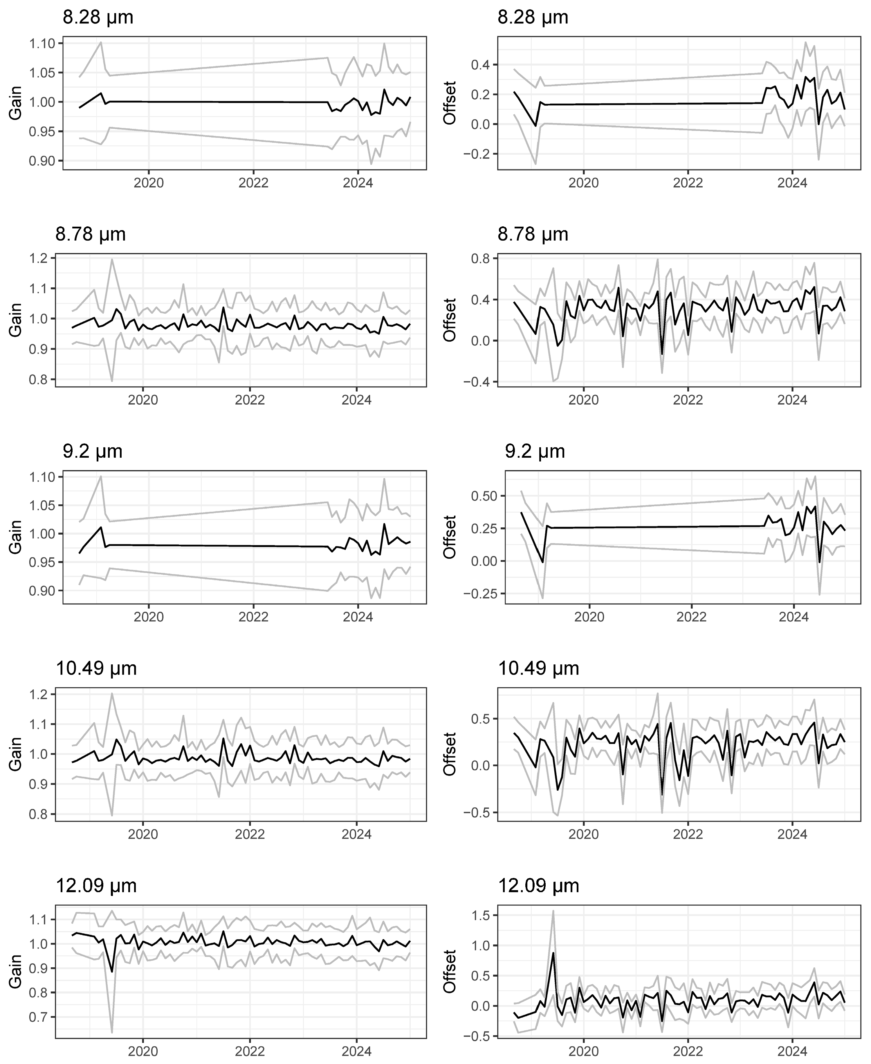
Temporal stability of monthly correction coefficients over the period of 2018–2024 is shown in Figure 8. Correction coefficients varied among months but the rates of change were not significantly different from zero except in the 12.09 µm band. The 12.09 µm band gain showed a significant decrease of 0.3% per year (uncertainty 0.1%) and a significant offset increase of 23 mK per year (uncertainty 8 mK). There is no indication of seasonality in any wavelength band. The origin of the month-to-month variability in the coefficients is not known.

4. Discussion

We used ECOSTRESS as the testbed for a proof-of-concept on-orbit cross-calibration and harmonization method for ultra-high-spatial-resolution TIR instruments, based on GSICS (Global Space-based Inter-Calibration System) [1]. The Infrared Atmospheric Sounding Interferometer (IASI) was used as the reference instrument [31]. Although the traceability chain to an SI radiance standard was broken by the launch of IASI [31], its high stability and accuracy have been used to justify its use as an on-orbit calibration standard [20,25,58].

The GSICS method and its variants have been used in a variety of calibration and harmonization activities. IASI and the similar CrIS instrument have been used as standards for harmonization of data from geostationary satellites [1] and performance evaluation of operational Sensor Data Records for polar satellites [59,60,61]. Other reference sensors like the Advanced Along-Track Scanning Radiometer (AATSR) and the Sea and Land Surface Temperature Radiometer (SLSTR) were used in the production of a Sea Surface Temperature Climate Data Record for the Satellite Era (1981–2025) [8,10]. These harmonization and calibration activities have largely been carried out on data from sensors with 0.75–4 km spatial resolution and detector noise levels less than 0.3 K. The new ultra-high-resolution sensors have much finer spatial resolution and higher noise levels.

Ultra-high-resolution TIR data come with a radiometric noise penalty because detector integration times are extremely short, especially in push-whisk instruments like ECOSTRESS. Spatial and temporal radiometric noise in ECOSTRESS is an order of magnitude larger than MODIS [62,63] and VIIRS [64,65,66] and nearly two orders of magnitude larger than SLSTR [67], all of which have an approximately 1 km spatial resolution. The future TRISHNA [68], LSTM [69] and SBG [70] missions are all expected to have radiometric noise levels similar to ECOSTRESS [14,71]. TRISHNA, LSTM, and SBG are planned as a virtual constellation, supplemented by ECOSTRESS, which will provide global daily coverage at a 50–60 m resolution on land and coastal waters. The three new missions will extend the ECOSTRESS 70 m resolution data record by a decade. The utility of such a constellation depends upon harmonized radiance acquisitions, based on a unified definition of “truth.” Therefore, it is important to determine whether the correction and harmonization approach was feasible for ECOSTRESS, which has noise levels much higher than many current operational sensors.

Recalibration of ECOSTRESS radiances was necessary. ECOSTRESS Collection 1 had a well-documented cold bias in all bands [11,12,13,14,15], so users who have an archive of Collection 1 data would benefit from a way to recalibrate their data without downloading a complete set of new files. Collection 2 is the currently available version of ECOSTRESS and has a smaller mean bias, but there is a temperature dependence of the bias, with a warm bias in cold scenes and a cold bias in warm scenes (Figure 2, Figure 3 and Figure 4) [17]. ECOSTRESS Collection 3 is in the testing stage as of February 2026, and the initial plan is to use the Collection 2 calibration, which will retain the negative temperature dependence of the bias. Therefore, it is likely that ECOSTRESS Collection 3 will have temperature-dependent biases, which will need correction. The ECOSTRESS L1B radiance biases propagate to all higher-level products, including L2 surface temperature and emissivity, L3 evapotranspiration, and others, so radiance bias correction is important to the entire community that uses ECOSTRESS data. Examples of the need for radiance bias correction include the cold bias in L2 surface temperature retrievals over water in both Collections 1 and 2 [12,14,72,73], and overestimation of L3 evapotranspiration (which scales inversely with temperature) in Collection 1 [74,75].

This paper provides correction coefficients to reduce both the median bias in each channel and the temperature dependence of that bias (Figure 2, Figure 3 and Figure 4; Table 3 and Table 4). These corrections greatly reduce the biases that are present in the operational ECOSTRESS radiance products that have been released to the public by JPL (Table 6 and Table 7, Figure 2, Figure 3 and Figure 4). The corrections also dramatically reduce the temperature dependence of the biases in ECOSTRESS products. This is especially important for ECOSTRESS Collection 2, which has much larger temperature dependencies of the biases than were present in Collection 1.

Our corrections led to calibration improvement similar to others reported in the literature. Mittaz and Harris [76] performed an IASI-based recalibration of AVHRR that reduced the mean AVHRR−IASI bias to less than 12 mK and the temperature dependence of the bias to between 0.0002 and 0.0004. Before correction, biases at 290 to 300 K were 500 mK in the 11 µm channel and 300 mK in the 12 µm band, and the temperature dependence was between 0.009 and 0.01. The uncorrected AVHRR biases were much smaller than what we have observed with ECOSTRESS Collection 1, and the uncorrected temperature dependence was approximately 10% of the ECOSTRESS Collection 1 value. Our biases after correction are on the order of 0.1 K, larger than Mittaz and Harris but within the range of operational VIIRS biases [77,78]. After correction, our ECOSTRESS temperature dependences are within the same range as Mittaz and Harris.

We suspect that detector nonlinearities in ECOSTRESS contribute to the temperature dependence of the biases, because some nonlinearities are evident in pre-launch vacuum chamber tests of ECOSTRESS [79]. ECOSTRESS uses HgCdTe detectors that have well-known nonlinearities [55,80], but radiance calibration is linear, based on the measurement of onboard black bodies at 293 K and 319 K during each mirror scan. In contrast, other instruments with HgCdTe detectors, including ASTER [81], AVHRR [4], MODIS [82], SLSTR [83] and VIIRS [78], all use quadratic terms in the calibration equations based either on preflight testing or on-orbit measurements. Overcorrection or undercorrection can lead to positive or negative temperature dependence of the bias [84], which might explain the difference between the signs of the temperature dependence in ECOSTRESS Collections 1 and 2.

The uncertainties of our corrections are higher than others reported in the literature, most likely due to the high levels of detector noise in ECOSTRESS and to instability of the ISS platform on which it is mounted. Hewison and collaborators [1,25] carried out an IASI correction of radiances for the geostationary SEVIRI imager. The combined uncertainties of their correction were between 12 and 13 mK. ECOSTRESS correction uncertainties (Table 17) are on the order of 20 to 50 mK, between two and four times larger than the SEVIRI correction uncertainties. There are several reasons for the larger ECOSTRESS uncertainties. The typical matchups between IASI and SEVIRI had time differences of less than 5 min. This is possible because SEVIRI is geostationary, so the temporal mismatch is limited only by the 5 min sampling interval of high-rate SEVIRI acquisitions. The median temporal mismatch in our IASI matchups was 13 min, nearly three times larger than the maximum mismatch in the SEVIRI matchups. ECOSTRESS Geolocation errors are large compared to SEVIRI because the ISS has an unstable orbit, and the ISS is not rigid so movements of the solar panels, and movement of personnel within the station, cause ECOSTRESS pointing errors. ECOSTRESS also has spatial noise levels of 300 to 600 mK and temporal noise levels of 60 to 500 mK depending on the wavelength and temperature [14]. SEVIRI spatial and temporal noise is on the order of 0.5 to 5 mK, and spatial and temporal mismatch uncertainty is on the order of 10 to 50 mK, all lower than the equivalent ECOSTRESS uncertainties (Table 13, Table 14, Table 15, Table 16 and Table 17).

Our validation with three different strictly independent datasets confirmed that the corrections reduced the median biases to 0.1 K, a big improvement compared biases in ECOSTRESS Collections 1 and 2 (Table 6, Table 7, Table 8, Table 9, Table 10 and Table 11). It also confirmed that the corrections reduced the temperature dependence of the biases to 0.005 or less (Table 5, Table 6, Table 7, Table 8, Table 9 and Table 10). The comparisons with IASI and CrIS are more robust than the comparison with RTTOV simulations for several reasons. The number of ECOSTRESS pixels in each IASI or CrIS comparison ranged from N = 10⁴ to 3 × 10⁴, so the standard error of the estimate of the ECOSTRESS radiance is on the order of RSD(radiance)/√(10⁴). In contrast, in the RTTOV comparisons, ECOSTRESS radiance was measured from nine pixels centered on the matchup location, so the standard error is RSD(radiance)/3. This means that the uncertainties of the ECOSTRESS radiances and their biases are much larger than in the IASI and CrIS comparisons. In addition, the RTTOV simulations use hourly meteorological reanalysis data that are gridded at a 25 km spatial scale, so the uncertainties due to spatial and temporal mismatch are larger than in the IASI and CrIS comparisons. However, despite the larger uncertainties in the RTTOV comparisons, they mirror the results of the IASI and CrIS comparisons.

ECOSTRESS calibration appears to have been relatively stable, with rates of calibration change that are not significantly different from zero in four of five bands (Figure 8). The offset drift in the 12.09 µm band was 23 mK per year. There are no clear signs of seasonality, but we are limited by the number of matchups available per month. This stability is good, especially considering that the thermal variability of ISS is high and ECOSTRESS depends on coolant from the ISS to maintain the temperature of the cold onboard black body. Among operational sensors, MODIS and VIIRS have been very stable. Aqua MODIS 11.03 and 12.04 µm bands have drifted at a rate of 10.5 and 10.7 mK per year over the period of 2003 to 2017 [85]. VIIRS on S-NPP gain varied by less than 1% over 9 years, and VIIRS on N-20 was more stable, with gain changes of less than 0.2% over 3 years. The exception was the 11.5 µm band, which degraded by 2.5% over 9 years (S-NPP) and by 1% over 3 years (N-20) [78]. In contrast, an analysis of multiple geostationary imagers during 2008 to 2012 [1] documented seasonal bias cycles ranging in amplitude from 0.01 K to 4 K.

The uncertainties associated with the correction are less than 0.05 K (Table 17), which is approximately the same order of magnitude as the uncertainty of the IASI data themselves [24,56]. The results of the validation confirm that our calibration correction is a major improvement over the corrections produced by JPL. They also confirm that our proof of concept is a potential method for the harmonization of radiance acquisitions from the future constellation of 50–70 m spatial resolution TIR imagers planned for the second half of the decade of the 2020s.

5. Conclusions

The aim of this work was to provide validated L1B radiance correction coefficients for ECOSTRESS Collections 1 and 2 that could be used on land or water. We used IASI as an on-orbit radiance standard for comparison with ECOSTRESS during quasi simultaneous overpasses. Estimates of uncertainties are provided. Results were validated by strictly independent matchups to IASI, CrIS and RTTOV radiative transfer simulations.

The work serves as a proof of concept for GSICS-based calibration and harmonization of radiances from ECOSTRESS and the future planned virtual constellation of 50 to 60 m spatial scale wide-swath TIR satellite instruments (TRISHNA, LSTM, SBG). Harmonization of calibration is essential for the constellation goal to provide daily global TIR data at an ultra-high spatial resolution.

References

1. Hewison, T.J.; Wu, X.; Yu, F.; Tahara, Y.; Hu, X.; Kim, D.; Koenig, M. GSICS Inter-Calibration of Infrared Channels of Geostationary Imagers Using Metop/IASI. IEEE Trans. Geosci. Remote Sens. 2013, 51, 1160–1170. [Google Scholar] [CrossRef] [Scilit]
2. Xu, N.; Chen, L.; Hu, X.; Zhang, L.; Zhang, P. Assessment and Correction of On-Orbit Radiometric Calibration of FY-3 VIRR Thermal Infrared Channels. Remote Sens. 2014, 6, 2884–2897. [Google Scholar] [CrossRef] [Scilit]
3. Liu, M.; Guan, L.; Liu, J.; Song, Q.; Ma, C.; Li, N. First Assessment of HY-1 COCTS Thermal Infrared Calibration Using MetOP-B IASI. Remote Sens. 2021, 13, 635. [Google Scholar] [CrossRef] [Scilit]
4. Chang, T.; Wu, X.; Weng, F. Modeling Thermal Emissive Bands Radiometric Calibration Impact with Reference to AVHRR. J. Geophys. Res. Atmos. 2017, 122, 2831–2843. [Google Scholar] [CrossRef] [Scilit]
5. Turpie, K.R.; Casey, K.A.; Crawford, C.J.; Guild, L.S.; Kieffer, H.; Lin, G.; Kokaly, R.; Shrestha, A.K.; Anderson, C.; Chandra, S.N.R.; et al. Calibration and Validation for the Surface Biology and Geology (SBG) Mission Concept: Recommendations for a Multi-Sensor System for Imaging Spectroscopy and Thermal Imagery. J. Geophys. Res. Biogeosciences 2023, 128, e2023JG007452. [Google Scholar] [CrossRef] [Scilit]
6. Thompson, J.O.; Williams, D.B.; Ramsey, M.S. The Expectations and Prospects for Quantitative Volcanology in the Upcoming Surface Biology and Geology (SBG) Era. Earth Space Sci. 2023, 10, e2022EA002817. [Google Scholar] [CrossRef] [Scilit]
7. Stavros, E.N.; Chrone, J.; Cawse-Nicholson, K.; Freeman, A.; Glenn, N.F.; Guild, L.S.; Kokaly, R.; Lee, C.; Luvall, J.; Pavlick, R.; et al. Designing an Observing System to Study the Surface Biology and Geology (SBG) of the Earth in the 2020s. J. Geophys. Res. Biogeosciences 2022, 128, e2021JG006471. [Google Scholar] [CrossRef] [Scilit]
8. Merchant, C.J.; Embury, O.; Bulgin, C.E.; Block, T.; Corlett, G.K.; Fiedler, E.; Good, S.A.; Mittaz, J.; Rayner, N.A.; Berry, D.; et al. Satellite-Based Time-Series of Sea-Surface Temperature since 1981 for Climate Applications. Sci Data 2019, 6, 223. [Google Scholar] [CrossRef] [Scilit]
9. Giering, R.; Quast, R.; Mittaz, J.P.D.; Hunt, S.E.; Harris, P.M.; Woolliams, E.R.; Merchant, C.J. A Novel Framework to Harmonise Satellite Data Series for Climate Applications. Remote Sens. 2019, 11, 1002. [Google Scholar] [CrossRef] [Scilit]
10. Merchant, C.J.; Block, T.; Corlett, G.K.; Embury, O.; Mittaz, J.P.D.; Mollard, J.D.P. Harmonization of Space-Borne Infra-Red Sensors Measuring Sea Surface Temperature. Remote Sens. 2020, 12, 1048. [Google Scholar] [CrossRef] [Scilit]
11. Hook, S.J.; Cawse-Nicholson, K.; Barsi, J.; Radocinski, R.; Hulley, G.C.; Johnson, W.R.; Rivera, G.; Markham, B. In-Flight Validation of the ECOSTRESS, Landsats 7 and 8 Thermal Infrared Spectral Channels Using the Lake Tahoe CA/NV and Salton Sea CA Automated Validation Sites. IEEE Trans. Geosci. Remote Sens. 2020, 58, 1294–1302. [Google Scholar] [CrossRef]
12. Shi, J.; Hu, C. Evaluation of ECOSTRESS Thermal Data over South Florida Estuaries. Sensors 2021, 21, 4341. [Google Scholar] [CrossRef] [Scilit]
13. Weidberg, N.; Wethey, D.S.; Woodin, S.A. Global Intercomparison of Hyper-Resolution ECOSTRESS Coastal Sea Surface Temperature Measurements from the Space Station with VIIRS-N20. Remote Sens. 2021, 13, 5021. [Google Scholar] [CrossRef] [Scilit]
14. Wethey, D.S.; Weidberg, N.; Woodin, S.A.; Vazquez-Cuervo, J. Characterization and Validation of ECOSTRESS Sea Surface Temperature Measurements at 70 m Spatial Scale. Remote Sens. 2024, 16, 1876. [Google Scholar] [CrossRef] [Scilit]
15. Hulley, G.C.; Gottsche, F.M.; Rivera, G.; Hook, S.J.; Freepartner, R.J.; Martin, M.A.; Cawse-Nicholson, K.; Johnson, W.R. Validation and Quality Assessment of the ECOSTRESS Level-2 Land Surface Temperature and Emissivity Product. IEEE Trans. Geosci. Remote Sens. 2022, 60, 1–23. [Google Scholar] [CrossRef] [Scilit]
16. Smyth, M.M.; Logan, T.L. ECOSTRESS Level 1 Product User Guide Version 3; Jet Propulsion Laboratory: La Cañada Flintridge, CA, USA, 2022. Available online: https://ecostress.jpl.nasa.gov/downloads/userguides/1_ECOSTRESS_L1_UserGuide_20190619.pdf (accessed on 10 February 2026).
17. Zhang, H.; Mahmood, A.N.; Hu, T.; Mallick, K.; Didry, Y.; Hitzelberger, P.; Szantoi, Z.; Pérez-Planells, L.; Göttsche, F.M.; Hulley, G.C.; et al. Global Evaluation of High-Resolution ECOSTRESS Land Surface Temperature and Emissivity Products: Collection 1 versus Collection 2. Remote Sens. Environ. 2025, 326, 114779. [Google Scholar] [CrossRef] [Scilit]
18. WMO. Global Space-based Inter-Calibration System (GSICS). Available online: https://gsics.wmo.int (accessed on 10 February 2026).
19. JPL ECOSTRESS. Algorithm Theoretic Basis Documents, Product Specification Documents & User Guides. Available online: https://ecostress.jpl.nasa.gov/data/atbds-summary-table (accessed on 10 February 2026).
20. Hewison, T. ATBD for EUMETSAT Operational GSICS Inter-Calibration of Meteosat-IASI; EUMETSAT: Darmstadt, Germany, 2015. [Google Scholar] [CrossRef] [Scilit]
21. Logan, T.L.; Johnson, W.R. ECOSTRESS Level-1 Focal Plane Array and Radiometric Calibration Algorithm Theoretical Basis Document; Jet Propulsion Laboratory: La Cañada Flintridge, CA, USA, 2018. Available online: https://lpdaac.usgs.gov/documents/222/ECO1B_Calibration_ATBD_V1.pdf (accessed on 10 February 2026).
22. Cha, J.; Carroll, B.; Rodriguez, J.; Maynard, K.; Romero, M. Thermal Design and On-Orbit Performance of the ECOSTRESS Instrument. In Proceedings of the Advances in Cryogenic Engineering, Hartford, CT, USA, 21–25 July 2019; IOP Publishing: Bristol, UK, 2020; Volume 755, p. 012005. [Google Scholar] [CrossRef] [Scilit]
23. Blumstein, D.; Chalon, G.; Carlier, T.; Buil, C.; Hébert, P.; Maciaszek, T.; Ponce, G.; Phulpin, T.; Tournier, G.; Siméoni, D.; et al. IASI Instrument: Technical Overviw and Measured Performance. In Proceedings of the SPIE, Denver, CO, USA, 4 November 2004; SPIE: Bellingham, WA, USA, 2004; Volume 5543, pp. 196–207. [Google Scholar] [CrossRef] [Scilit]
24. Kilymis, D.; Kangah, Y.; Le Barbier, L.; Jacquette, E.; Lenot, X.; Ansart, J.; Faillot, M.; Calvel, J.-C.; Codou, G.; Vandermarcq, O. IASI Global Radiometric Uncertainty Budget. Atmos. Meas. Tech. 2025, 18, 6513–6525. [Google Scholar] [CrossRef] [Scilit]
25. Hewison, T.J. An Evaluation of the Uncertainty of the GSICS SEVIRI-IASI Intercalibration Products. IEEE Trans. Geosci. Remote Sens. 2013, 51, 1171–1181. [Google Scholar] [CrossRef] [Scilit]
26. Tobin, D.; Revercomb, H.E.; Knuteson, R.; Taylor, J.; Best, F.; Borg, L.; DeSlover, D.; Martin, G.; Buijs, H.; Esplin, M.; et al. Suomi-NPP CrIS Radiometric Calibration Uncertainty. J. Geophys. Res. Atmos. 2013, 118, 10589–10600. [Google Scholar] [CrossRef] [Scilit]
27. Hocking, J.; Rayer, P.; Rundle, D.; Saunders, R.; Matricardi, M.; Geer, A.; Brunel, P.; Vidot, J. RTTOV V12 Users Guide; EUMETSAT NWP SAF: Exeter, UK, 2019; Available online: https://nwp-saf.eumetsat.int/site/download/documentation/rtm/docs_rttov12/users_guide_rttov12_v1.3.pdf (accessed on 10 February 2026).
28. Xu, F.; Ignatov, A. iQuam in Situ SST Quality Monitor v2.10. Available online: https://www.star.nesdis.noaa.gov/socd/sst/iquam/data.html (accessed on 10 February 2026).
29. European Centre for Medium-Range Weather Forecasts ERA5 Reanalysis (0.25 Degree Latitude-Longitude Grid); NSF National Center for Atmospheric Research: Boulder, CO, USA, 2015. [CrossRef]
30. Saunders, R.; Hocking, J.; Rundle, D.; Rayer, P.; Havemann, S.; Matricardi, M.; Geer, A.; Lupu, C.; Brunel, P.; Vidot, J. RTTOV-12 Science and Validation Report; EUMETSAT NWP SAF: Exeter, UK, 2017; Available online: https://nwp-saf.eumetsat.int/site/download/documentation/rtm/docs_rttov12/rttov12_svr.pdf (accessed on 10 February 2026).
31. EUMETSAT. GSICS Traceability Statement for IASI and AIRS; EUMETSAT: Darmstadt, Germany, 2014; Available online: https://user.eumetsat.int/s3/eup-strapi-media/pdf_trace_stat_iasi_airs_b3b3232020.pdf (accessed on 10 February 2026).
32. EUMETSAT. EUMETSAT Data Store. Available online: https://data.eumetsat.int/ (accessed on 10 February 2026).
33. EUMETSAT. EUMETSAT Data Access Client. Available online: https://user.eumetsat.int/resources/user-guides/eumetsat-data-access-client-eumdac-guide (accessed on 10 February 2026).
34. EUMETSAT. Data Tailor. Available online: https://user.eumetsat.int/resources/user-guides/data-tailor-standalone-guide (accessed on 10 February 2026).
35. EUMETSAT. IASI Level 1: Product Guide; EUMETSAT: Darmstadt, Germany, 2019; Available online: https://user.eumetsat.int/s3/eup-strapi-media/pdf_iasi_pg_487c765315.pdf (accessed on 4 February 2026).
36. UW-SSEC. Snotimes-Times and Locations of Near-Simultaneous Intersection of 2 Satellites. Available online: https://sips.ssec.wisc.edu/orbnav#/tools/snotimes (accessed on 10 February 2026).
37. EUMETSAT. EUMETSAT API. Available online: https://api.eumetsat.int/data/search-products/1.0.0/os?format=json&pi=EO:EUM:DAT:METOP:IASIL1C-ALL (accessed on 10 February 2026).
38. EUMETSAT. IASI Level 2: Product Generation Specification; EUMETSAT: Darmstadt, Germany, 2017; Available online: https://user.eumetsat.int/s3/eup-strapi-media/IASI_Level_2_Product_Generation_Specification_4676b85e0f.pdf (accessed on 10 February 2026).
39. Pebesma, E.; Bivand, R. Spatial Data Science: With Applications in R; Chapman & Hall: London, UK, 2023. [Google Scholar]
40. Cao, C.; Heidinger, A.K. Inter-Comparison of the Longwave Infrared Channels of MODIS and AVHRR/NOAA-16 Using Simultaneous Nadir Observations at Orbit Intersections. Proceedings of SPIE, Seattle, WA, USA, 24 September 2002; SPIE: Bellingham, WA, USA, 2002; Volume 4814, pp. 306–316. [Google Scholar] [CrossRef] [Scilit]
41. Gunshor, M.M. Converting Advanced Himawari Imager (AHI) Radiance Units; Cooperative Institute for Meteorological Satellite Studies (CIMSS): Madison, WI, USA, 2015; Available online: https://cimss.ssec.wisc.edu/goes/calibration/Converting_AHI_RadianceUnits_24Feb2015.pdf (accessed on 10 February 2026).
42. Padula, F.; Cao, C. CWG Analysis: ABI Max/Min Radiance Characterization and Validation; Cooperative Institute for Meteorological Satellite Studies (CIMSS): Madison, WI, USA, 2011; Available online: https://cimss.ssec.wisc.edu/goes/calibration/ABI_maxMin_Radiance_MEMO_V2_04March2011_update.pdf (accessed on 10 February 2026).
43. Hulley, G. ECOSTRESS Spectral Response Functions V3; Jet Propulsion Laboratory: La Cañada Flintridge, CA, USA, 2018. Available online: https://ecostress.jpl.nasa.gov/downloads/srf/20180318-ECOSTRESS_SRF_v3.xlsx (accessed on 10 February 2026).
44. Di, D.; Min, M.; Li, J.; Gunshor, M.M. The Radiance Differences between Wavelength and Wavenumber Spaces in Convolving Hyperspectral Infrared Sounder Spectrum to Broadband for Intercomparison. Remote Sens. 2019, 11, 1177. [Google Scholar] [CrossRef] [Scilit]
45. LPDAAC. ECOSTRESS Brightness Temperature Lookup Tables. Available online: https://git.earthdata.nasa.gov/projects/LPDUR/repos/ecostress_swath2grid/commits/dce71069dd6c03f2e245d2456bca7044caf897ae#EcostressBrightnessTemperatureV01.h5 (accessed on 10 February 2026).
46. Weinreb, M.P.; Fleming, H.E.; McMillin, L.M.; Neuendorffer, A.C. Transmittances for the TIROS Operational Vertical Sounder; U.S. Department of Commerce National Oceanic and Atmospheric Administration: Washington, DC, USA, 1981. Available online: https://repository.library.noaa.gov/view/noaa/13429/noaa_13429_DS1.pdf (accessed on 10 February 2026).
47. Hocking, J. A Visible/Infrared Multiple-Scattering Model for RTTOV; EUMETSAT NWP SAF: Exeter, UK, 2016; Available online: https://nwp-saf.eumetsat.int/publications/tech_reports/nwpsaf-mo-tr-031.pdf (accessed on 10 February 2026).
48. EUMETSAT-NWPSAF RTTOV Multispectral UV/VIS/IR Coefficients and Optical Properties: 54L V13 Predictor Variable O3+CO2 Files for All Supported Visible/IR Sensors; EUMETSAT NWP SAF: Exeter, UK, 2025; Available online: https://nwp-saf.eumetsat.int/downloads/rtcoef_rttov14/rttov13pred54L/rtcoef_visir_rttov13pred54L_o3co2.tar.bz2 (accessed on 10 February 2026).
49. Mittaz, J.P.D.; Harris, A.R.; Sullivan, J.T. A Physical Method for the Calibration of the AVHRR/3 Thermal IR Channels 1: The Prelaunch Calibration Data. J. Atmos. Ocean. Technol. 2009, 26, 996–1019. [Google Scholar] [CrossRef] [Scilit]
50. Tobin, D.C.; Revercomb, H.E.; Moeller, C.C.; Pagano, T.S. Use of Atmospheric Infrared Sounder High–Spectral Resolution Spectra to Assess the Calibration of Moderate Resolution Imaging Spectroradiometer on EOS Aqua. J. Geophys. Res. 2006, 111, D09S05. [Google Scholar] [CrossRef] [Scilit]
51. Veglio, P.; Tobin, D.C.; Dutcher, S.; Quinn, G.; Moeller, C.C. Long-Term Assessment of Aqua MODIS Radiance Observation Using Comparisons with AIRS and IASI. J. Geophys. Res. Atmos. 2016, 121, 8460–8471. [Google Scholar] [CrossRef] [Scilit]
52. QGIS. QGIS Version 3.14.16, 2024. Available online: https://qgis.org/ (accessed on 10 February 2026).
53. Wu, W.; Liu, X.; Li, Y.; Yang, Q.; Wu, A.; Kizer, S.; Cao, C. An Accurate Method for Correcting Spectral Convolution Errors in Intercalibration of Broadband and Hyperspectral Sensors. J. Geophys. Res. Atmos. 2018, 123, 9238–9255. [Google Scholar] [CrossRef] [Scilit]
54. Johnson, W.R.; Hook, S.J.; Schmitigal, W.; Goullioud, R. ECOSTRESS End-to-End Radiometric Pre-Flight Calibration and Validation. In Proceedings of the 2018 SPIE Conference on Optical Engineering + Applications Conference, San Diego, CA, USA, 18 September 2018; SPIE: Bellingham, WA, USA, 2018. [Google Scholar] [CrossRef] [Scilit]
55. Walton, C.C.; Sullivan, J.T.; Rao, C.R.N.; Weinreb, M.P. Corrections for Detector Nonlinearities and Calibration Inconsistencies of the Infrared Channels of the Advanced Very High Resolution Radiometer. J. Geophys. Res. 1998, 103, 3323–3337. [Google Scholar] [CrossRef] [Scilit]
56. Loveless, M.; Knuteson, R.; Revercomb, H.E.; Borg, L.; DeSlover, D.; Martin, G.; Taylor, J.; Iturbide-Sanchz, F.; Tobin, D.C. Comparison of the AIRS, IASI, and CrIS Infrared Sounders Using Simultaneous Nadir Overpasses: Novel Methods Applied to Data From 1 October 2019 to 1 October 2020. Earth Space Sci. 2023, 10, e2023EA002878. [Google Scholar] [CrossRef] [Scilit]
57. Xu, F.; Ignatov, A. In Situ SST Quality Monitor (iQuam). J. Atmos. Ocean. Technol. 2014, 31, 164–180. [Google Scholar] [CrossRef] [Scilit]
58. Chander, G.; Hewison, T.J.; Fox, N.; Wu, X.; Xiong, X.; Blackwell, W.J. Overview of Intercalibration of Satellite Instruments. IEEE Trans. Geosci. Remote Sens. 2013, 51, 1056–1080. [Google Scholar] [CrossRef] [Scilit]
59. Cao, C.; Zhang, B.; Shao, X.; Wang, W.; Uprety, S.; Choi, T.; Blonski, S.; Gu, Y.; Bai, Y.; Lin, L.; et al. Mission-Long Recalibrated Science Quality Suomi NPP VIIRS Radiometric Dataset Using Advanced Algorithms for Time Series Studies. Remote Sens. 2021, 13, 1075. [Google Scholar] [CrossRef] [Scilit]
60. Wang, W.; Cao, C.; Blonski, S.; Gu, Y.; Zhang, B.; Uprety, S.; Choi, T.; Shao, X. NOAA-20/S-NPP VIIRS Sensor Data Record on-Orbit Performance Updates and Recent Improvements. In Proceedings of the IGARSS 2020—2020 IEEE International Geoscience and Remote Sensing Symposium, Waikoloa, HI, USA, 26 September–2 October 2020; IEEE: New York City, NY, USA; pp. 6389–6392. [Google Scholar] [CrossRef] [Scilit]
61. Chang, T.; Xiong, X.; Shrestha, A.; Diaz, C.P. Normalization Method and Application for MODIS TEB Assessments Using Earth Scene Measurements. Earth Space Sci. 2021, 8, e2020EA001539. [Google Scholar] [CrossRef] [Scilit]
62. Madhavan, S.; Xiong, X.; Wu, A.; Wenny, B.N.; Chiang, K.; Chen, N.; Wang, Z.; Li, Y. Noise Characterization and Performance of MODIS Thermal Emissive Bands. IEEE Trans. Geosci. Remote Sens. 2016, 54, 3221–3234. [Google Scholar] [CrossRef] [Scilit]
63. Bouali, M.; Ignatov, A. Estimation of Detector Biases in MODIS Thermal Emissive Bands. IEEE Trans. Geosci. Remote Sens. 2013, 51, 4339–4348. [Google Scholar] [CrossRef]
64. Wang, Z.; Cao, C. Assessing the Effects of Suomi NPP VIIRS M15/M16 Detector Radiometric Stability and Relative Spectral Response Variation on Striping. Remote Sens. 2016, 8, 145. [Google Scholar] [CrossRef] [Scilit]
65. Oudrari, H.; McIntire, J.; Xiong, X.; Butler, J.; Ji, Q.; Schwarting, T.; Lee, S.; Efremova, B. JPSS-1 VIIRS Radiometric Characterization and Calibration Based on Pre-Launch Testing. Remote Sens. 2016, 8, 41. [Google Scholar] [CrossRef] [Scilit]
66. Pérez Díaz, C.L.; Xiong, X.; Li, Y.; Chiang, K. S-NPP VIIRS Thermal Emissive Bands 10-Year On-Orbit Calibration and Performance. Remote Sens. 2021, 13, 3917. [Google Scholar] [CrossRef] [Scilit]
67. Smith, D.; Hunt, S.E.; Etxaluze, M.; Peters, D.; Nightingale, T.; Mittaz, J.; Woolliams, E.R.; Polehampton, E. Traceability of the Sentinel-3 SLSTR Level-1 Infrared Radiometric Processing. Remote Sens. 2021, 13, 374. [Google Scholar] [CrossRef] [Scilit]
68. Charvet, D.; Gnata, X.; Toulemont, A.; Rizzolo, S.; Clénet, A.; Libouban, C.; Gossant, A.; Chassat, F.; Buffet, L.; Salcedo, C.; et al. TRISHNA TIR Instrument Development and Performance Status. In Proceedings of the the International Conference on Space Optics—ICSO 2022, Dubrovnik, Croatia, 12 July 2023; Minoglou, K., Karafolas, N., Cugny, B., Eds.; SPIE: Bellingham, WA, USA, 2022; Volume 12777, p. 1277742. [Google Scholar] [CrossRef] [Scilit]
69. Bernard, F.; Bourgeois, G.; Manolis, I.; Barat, I.; Bolea Alamanac, A.; Such Taboada, M.; Mingorance, P.; Ciapponi, A.; Cardone, T.; Dutruel, E.; et al. The LSTM Instrument: Design, Technology and Performance. In Proceedings of the International Conference on Space Optics—ICSO 2022, Dubrovnik, Croatia, 12 July 2023; Minoglou, K., Karafolas, N., Cugny, B., Eds.; SPIE: Bellingham, WA, USA, 2023; Volume 12777, p. 1277740. [Google Scholar] [CrossRef] [Scilit]
70. Basilio, R.R.; Hook, S.J.; Zoffoli, S.; Buongiorno, M.F. Surface Biology and Geology (SBG) Thermal Infrared (TIR) Free -Flyer Concept. In Proceedings of the 2022 IEEE Aerospace Conference (AERO), Big Sky, MT, USA, 5 March 2022; IEEE: New York City, NY, USA, 2022; pp. 1–9. [Google Scholar] [CrossRef] [Scilit]
71. Liberti, G.L.; Sabatini, M.; Wethey, D.S.; Ciani, D. A Multi-Pixel Split-Window Approach to Sea Surface Temperature Retrieval from Thermal Imagers with Relatively High Radiometric Noise: Preliminary Studies. Remote Sens. 2023, 15, 2453. [Google Scholar] [CrossRef] [Scilit]
72. Gustine, R.N.; Lee, C.M.; Halverson, G.H.; Acuna, S.C.; Cawse-Nicholson, K.A.; Hulley, G.C.; Hestir, E.L. Using ECOSTRESS to Observe and Model Diurnal Variability in Water Temperature Conditions in the San Francisco Estuary. IEEE Trans. Geosci. Remote Sens. 2022, 60, 4205710. [Google Scholar] [CrossRef] [Scilit]
73. Longenecker, J.; Benzoni, F.; Dunn, N.; Fox, H.E.; Gleason, A.; Otis, D.; Chirayath, V.; Oury, N.; Purkis, S.J. Coral Reef Thermal Microclimates Mapped from the International Space Station. Coral Reefs 2025, 44, 381–398. [Google Scholar] [CrossRef] [Scilit]
74. Hu, T.; Mallick, K.; Hitzelberger, P.; Didry, Y.; Boulet, G.; Szantoi, Z.; Koetz, B.; Alonso, I.; Pascolini-Campbell, M.; Halverson, G.; et al. Evaluating European ECOSTRESS Hub Evapotranspiration Products Across a Range of Soil-Atmospheric Aridity and Biomes Over Europe. Water Resour. Res. 2023, 59, e2022WR034132. [Google Scholar] [CrossRef] [Scilit]
75. Liang, L.; Feng, Y.; Wu, J.; He, X.; Liang, S.; Jiang, X.; De Oliveira, G.; Qiu, J.; Zeng, Z. Evaluation of ECOSTRESS Evapotranspiration Estimates over Heterogeneous Landscapes in the Continental US. J. Hydrol. 2022, 613, 128470. [Google Scholar] [CrossRef] [Scilit]
76. Mittaz, J.; Harris, A. A Physical Method for the Calibration of the AVHRR/3 Thermal IR Channels. Part II: An In-Orbit Comparison of the AVHRR Longwave Thermal IR Channels on Board MetOp-A with IASI. J. Atmos. Ocean. Technol. 2011, 28, 1072–1087. [Google Scholar] [CrossRef] [Scilit]
77. Wang, W.; Cao, C.; Blonski, S. NOAA-21 VIIRS Thermal Emissive Bands Early On-Orbit Calibration Performance and Improvements. IEEE Trans. Geosci. Remote Sens. 2024, 62, 5006313. [Google Scholar] [CrossRef] [Scilit]
78. Wang, W.; Cao, C. NOAA-20 and S-NPP VIIRS Thermal Emissive Bands On-Orbit Calibration Algorithm Update and Long-Term Performance Inter-Comparison. Remote Sens. 2021, 13, 448. [Google Scholar] [CrossRef] [Scilit]
79. Johnson, W.R.; Hook, S.J.; Schmitigal, W.P.; Gullioud, R.; Logan, T.L.; T.Lum, K. ECOSTRESS End-to-End Radiometric Validation. In Proceedings of the 2019 IEEE Aerospace Conference, Big Sky, MT, USA, 2–9 March 2019; IEEE: New York City, NY, USA, 2019; pp. 1–8. [Google Scholar] [CrossRef] [Scilit]
80. Theocharous, E.; Ishii, J.; Fox, N.P. Absolute Linearity Measurements on HgCdTe Detectors in the Infrared Region. Appl. Opt. 2004, 43, 4182. [Google Scholar] [CrossRef] [Scilit] [PubMed]
81. Arai, K.; Tonooka, H. Radiometric Performance Evaluation of ASTER VNIR, SWIR, and TIR. IEEE Trans. Geosci. Remote Sens. 2005, 43, 2725–2732. [Google Scholar] [CrossRef]
82. Xiong, X.; Angal, A.; Chang, T.; Chiang, K.; Lei, N.; Li, Y.; Sun, J.; Twedt, K.; Wu, A. MODIS and VIIRS Calibration and Characterization in Support of Producing Long-Term High-Quality Data Products. Remote Sens. 2020, 12, 3167. [Google Scholar] [CrossRef] [Scilit]
83. Smith, D.; Barillot, M.; Bianchi, S.; Brandani, F.; Coppo, P.; Etxaluze, M.; Frerick, J.; Kirschstein, S.; Lee, A.; Maddison, B.; et al. Sentinel-3A/B SLSTR Pre-Launch Calibration of the Thermal InfraRed Channels. Remote Sens. 2020, 12, 2510. [Google Scholar] [CrossRef] [Scilit]
84. Wu, X.; Yu, F. Correction for GOES Imager Spectral Response Function Using GSICS. Part I Theory IEEE Trans. Geosci. Remote Sens. 2013, 51, 1215–1223. [Google Scholar] [CrossRef]
85. Liu, T.-C.; Xiong, X.; Shao, X.; Chen, Y.; Wu, A.; Chang, T.; Shrestha, A. Evaluation of Aqua MODIS Thermal Emissive Bands Stability through Radiative Transfer Modeling. J. Appl. Rem. Sens. 2021, 15, 024502. [Google Scholar] [CrossRef] [Scilit]
Figure 1. Chart of workflow. Numbers in grey boxes refer to section numbers of the paper. Figure modified from [20].
Remotesensing 18 00622 g001
Figure 2. ECOSTRESS − IASI BT biases. Horizontal axis is IASI BT, vertical axis is ECOSTRESS − IASI BT bias relative to IASI. Blocks of 3 graphs are results for ECOSTRESS 8.28 and 8.78 µm bands. Colors indicate number of observations at each point on the graphs. Horizontal line indicates zero bias, dotted blue lines are regressions of bias versus temperature. Top graph in each block is the bias in ECOSTRESS Collection 1, second graph is the bias in ECOSTRESS Collection 2, third graph is the bias after independent IASI-derived correction.
Remotesensing 18 00622 g002
Figure 3. ECOSTRESS − IASI BT biases. Blocks of 3 graphs are results for ECOSTRESS 9.20 and 10.49 µm bands. Top graph in each block is the bias in ECOSTRESS Collection 1, second graph is the bias in ECOSTRESS Collection 2, third graph is the bias after independent IASI-derived correction. Axes, lines and colors as in Figure 2.
Remotesensing 18 00622 g003
Figure 4. ECOSTRESS − IASI BT biases. Block of 3 graphs are results for ECOSTRESS 12.09 µm band. Top graph is the bias in ECOSTRESS Collection 1, second graph is the bias in ECOSTRESS Collection 2, third graph is the bias after independent IASI-derived correction. Axes, lines and colors as in Figure 2.
Remotesensing 18 00622 g004
Figure 5. Validation of IASI results with independent comparison to CrIS hyperspectral observations. Horizontal axis is CrIS BT, vertical axis is ECOSTRESS − CrIS BT bias. Left column: 10.49 µm band, right column 12.09 µm band. First row: ECOSTRESS − CrIS brightness temperature biases in Collection 1, second row: ECOSTRESS − CrIS brightness temperature biases in Collection 2, third row: ECOSTRESS − CrIS brightness temperature biases after IASI-derived correction. Lines and colors as in Figure 2.
Remotesensing 18 00622 g005
Figure 6. Validation of IASI corrections with RTTOV radiative transfer simulations at independent triple matchups among ECOSTRESS, best-quality in situ observations from the NOAA iQuam database, and clear-sky geostationary observations. These matchups are described in [14]. Horizontal axis is RTTOV-simulated ECOSTRESS BT, vertical axis is ECOSTRESS − RTTOV BT bias. Lines and colors as in Figure 2. Vertical blocks of 3 graphs are for wavelengths 8.78 and 10.49 µm. Top row is the ECOSTRESS − RTTOV BT bias of Collection 1, second row is the ECOSTRESS − RTTOV BT bias of Collection 2, row three is the ECOSTRESS − RTTOV BT bias after IASI-derived correction.
Remotesensing 18 00622 g006
Figure 7. Validation of IASI corrections with RTTOV radiative transfer simulations at independent triple matchups among ECOSTRESS, best-quality in situ observations from the NOAA iQuam database, and cloud-free geostationary observations. These matchups are described in [14]. Vertical blocks of 3 graphs are for wavelength 12.09 µm. Top row is the ECOSTRESS − RTTOV BT bias of Collection 1, second row is the ECOSTRESS − RTTOV BT bias of Collection 2, row three is the ECOSTRESS − RTTOV BT bias after the IASI-derived correction. Axes, lines and colors as in Figure 6.
Remotesensing 18 00622 g007
Figure 8. Monthly time series of correction gain. Grey lines are ±1 SE.
Remotesensing 18 00622 g008