DDS-DeeplabV3+: A Lightweight Deformable Convolutional Network for Cloud Detection in Remote Sensing Imagery

Highlights

What are the main findings?

• Proposes a novel lightweight cloud detection model, DDS-DeeplabV3+. It enhances modeling capability for irregular cloud formations and complex boundaries by introducing deformable convolutions (DCN) and integrates a dual-branch collaborative mechanism (DCM) and a parameter-free attention module (SimAM).
• Experimental validation on Landsat-8 and GF-1 datasets demonstrates superior performance, achieving Mean Intersection over Union (MIoU) values of 92.61% and 94.04%, respectively, outperforming various mainstream comparison methods.

What is the implication of the main finding?

• Provides an effective solution for accurate cloud detection in complex scenarios. The model exhibits stronger robustness for thin clouds, broken clouds, and blurred cloud-ground boundaries, improving the usability of remote sensing data and the accuracy of downstream tasks.
• Achieves a favorable balance between accuracy and efficiency. The lightweight design of the backbone network maintains high performance while controlling computational complexity, making it more suitable for practical applications with limited resources.

Abstract

Cloud detection in remote sensing imagery is a research hotspot in the field of image processing, and accurately detecting and segmenting cloud regions is crucial for improving the utilization efficiency of remote sensing data. However, standard convolutional neural networks face limitations in modeling the complex spatial structures of clouds. To address these challenges, this paper proposes a cloud detection method based on DDS-DeeplabV3+. First, a lightweight design of the Xception network is adopted to control model complexity, and part of its standard convolutional layers are replaced with Deformable Convolutional Networks (DCN), which enhances the capability of the model to capture geometric features of irregular cloud formations. Second, a Dual-Branch Collaborative Mechanism (DCM) that integrates global context modeling with local detail perception is designed to reconstruct the Atrous Spatial Pyramid Pooling (ASPP) module, thereby improving performance in handling complex scenes and fine boundary delineation. Finally, the SimAM (Simple, Parameter-Free Attention Module) is incorporated into the decoder module, enhancing thin cloud detection capability. Experimental results on the Landsat-8 and GF-1 datasets show that the proposed model achieves Mean Intersection over Union (MIoU) values of 92.61% and 94.04%, respectively, outperforming other comparative methods and demonstrating its superior performance in cloud detection tasks.

1. Introduction

Satellite remote sensing technology is an essential method for observing the Earth’s surface from a distance, utilizing sensors mounted on satellite platforms. Remote sensing satellites employ multispectral and hyperspectral imagers, as well as radar sensors, to receive electromagnetic waves reflected or scattered by ground objects, acquiring image data across various bands including visible light, infrared, and microwave [1,2]. This technology offers advantages such as broad coverage, high spatial resolution, and the capability for time-series observations, making it widely applicable in meteorological forecasting, disaster assessment, agricultural resource surveys, urban planning, environmental protection, and other fields [3]. With continuous improvements in sensor accuracy and data processing capabilities, remote sensing has seen significant advancements in spatial, temporal, and spectral resolution, providing crucial support for the precise identification of surface targets and dynamic monitoring. However, observations from the International Satellite Cloud Climatology Project (ISCCP) indicate that the global annual average cloud coverage exceeds 67% [4], which frequently causes optical remote sensing images to be affected by cloud layers. On one hand, clouds themselves are important atmospheric parameters that reflect the state of atmospheric motion and reveal patterns of atmospheric environmental change, playing an irreplaceable role in weather forecasting and climate prediction [5,6]. On the other hand, cloud layers act as an invisible barrier, attenuating the radiative transfer of surface signals to varying degrees. This attenuation negatively impacts image quality and information completeness, increases the data transmission burden, and also affects application areas such as photovoltaic power generation and navigation safety. Therefore, accurate cloud detection is crucial for assessing image quality, alleviating the data transmission burden on satellite payloads [7,8], improving data utilization efficiency, and supporting downstream tasks [9,10].

Cloud detection is a critical step in remote sensing data processing, aiming to identify and segment cloud areas in images to enhance data integrity and usability. Due to the reflection and scattering characteristics of clouds, cloud regions often severely interfere with the extraction of surface information. Thus, accurately removing cloud-affected areas is essential for improving image utilization. Nonetheless, cloud detection faces numerous challenges, including diverse cloud morphologies (e.g., cirrus, cumulus, stratus), significant variations in thickness and transparency, and the easy confusion of cloud boundaries with certain surface features (e.g., snow, bright buildings) [11]. Current cloud detection technologies are primarily divided into two categories: traditional image processing-based methods, which utilize spectral and statistical features of cloud images, such as thresholding methods, multispectral fusion methods, and edge detection methods; and learning algorithm-based methods, such as convolutional neural networks (CNNs) and Transformers.

Early traditional methods primarily relied on spectral and statistical features, using techniques like threshold segmentation, multispectral fusion, and edge detection to distinguish clouds from surface targets. For instance, Zhu et al. improved the CFMask algorithm [12]. Foga et al. proposed a decision tree-based method to label pixels and generate cloud shadow masks by projecting estimated cloud heights onto the ground [13]. Zhang et al. proposed the Haze Optimized Transformation (HOT) for detecting and characterizing cloud spatial distribution [14], and Chen et al. developed a transformation method for detecting cloud and haze distribution in Landsat images by amplifying haze changes through spectral sensitivity [15]. However, these methods are largely based on fixed rules and are highly sensitive to cloud type, illumination, and atmospheric conditions, resulting in poor adaptability in complex scenarios.

With advances in deep learning, CNN-based cloud segmentation methods have gained attention due to their ability to automatically extract high-level features, improving accuracy in cloud morphology, texture, and edge detection. Classical semantic segmentation algorithms such as U-Net [16] and DeeplabV3 [17] have been applied to cloud detection tasks. Following the introduction of models like Transformers into the field, numerous Transformer-based cloud detection algorithms have emerged. Examples include MSCFF, which combines multi-scale convolutional features to facilitate cloud detection [18]. DBNet, which employs a hybrid model integrating Transformer and CNN to capture semantic and spatial details, thereby reducing false positives and negatives in cloud segmentation [19]. HRCloudNet, which uses a hierarchical integration approach to preserve cloud texture in high-resolution image segmentation [20], and MCDNet, which achieves effective cloud segmentation through multi-scale feature fusion [21]. Li et al. proposed the RDE-SegNeXt architecture, integrating RDEMSCA into the SegNeXt model based on gated linear units, combining parallel reparameterized convolution and detail enhancement convolution to enhance feature expression and edge detail capture for targets like clouds, shadows, and snow, enabling efficient cloud detection [22]. Li et al. also proposed RD-UNet, designing two U-shaped networks enhanced with residual connections to strengthen information flow, thereby optimizing the capture of detail and edge information, effectively promoting the utilization of multi-scale features, improving thin cloud detection capability, and distinguishing other interfering ground objects [23]. However, existing deep learning algorithms typically rely on standard convolutional neural networks. The spatial information and receptive fields learned by standard CNNs are confined to a fixed rectangular structure, lacking an inherent mechanism for handling geometric transformations, which presents limitations in modeling the complex spatial structures of clouds. To address the aforementioned challenges, this paper proposes a cloud detection method for satellite imagery based on DDS-DeeplabV3+. The main contributions of this work are summarized as follows:

1.

The Xception network, serving as the encoder backbone, is first lightweighted to control the overall model complexity, thereby reserving computational capacity for more sophisticated modules. Subsequently, part of its standard convolutional layers are replaced with DCN. This enhancement allows the model to adaptively adjust the shape and size of the receptive field, enabling more flexible and precise alignment with the highly irregular geometries of cloud formations. Consequently, the feature extraction capability for complex cloud spatial structures is significantly improved.

2.

A Dual-Branch Collaborative Mechanism is designed, integrating global context modeling and local detail perception, to reconstruct the original Atrous Spatial Pyramid Pooling module. The outputs of the dual branches interact through a feature fusion strategy, empowering the model to simultaneously leverage macro-level semantic information and micro-level boundary details. This design yields more accurate judgments in challenging scenarios characterized by dramatic variations in cloud thickness, transparency, or blurred boundaries.

3.

The SimAM is incorporated into the decoder module. SimAM can automatically focus on contrast edges between clouds and backgrounds such as land or sea, effectively enhancing the sensitivity of the model to low-contrast regions. It strengthens the focus of the decoder on critical information during detail restoration, ensuring effective responses to clouds at various scales.

2. Methodology

2.1. Overall Architecture of DDS-DeeplabV3+

This study selects Deeplabv3+ as the baseline model and proposes a novel satellite remote sensing image cloud detection algorithm named DDS-DeeplabV3+, aiming to address the limitations of standard convolutional neural networks in modeling complex cloud spatial structures due to their lack of an inherent mechanism for handling geometric transformations. The overall framework of the model is shown in Figure 1.

First, part of the convolutional layers in the Xception network are replaced with DCNs to enhance the model’s ability to extract features from irregular cloud formations. To further control computational complexity, the backbone feature extraction network is lightweighted before introducing the DCNs, preventing a significant increase in parameters. Second, a dual-branch interactive mechanism integrating global context modeling and local detail perception is designed to reconstruct the atrous spatial pyramid pooling module. This design enhances the model’s discriminative capability for cloud boundaries in complex scenarios, particularly strengthening the perception of thin clouds and fine cloud structures. Finally, the SimAM is incorporated into the decoder module. SimAM can automatically focus on boundary regions between clouds and the background, improving thin cloud detection capability. It effectively responds to clouds of various sizes, making it suitable for multi-scale cloud detection, and enhances the contrast features between clouds and the underlying surface, such as land and ocean.

2.2. Light-DCN-Xception

To address the limitations of standard convolutional neural networks in modeling the complex spatial structures of cloud clusters, this study replaces part of the convolutional layers in the Xception network with DCNs to enhance feature extraction capability. However, the introduction of deformable convolutions may increase computational costs. To balance model accuracy and inference efficiency in resource-constrained environments, a lightweight improvement is applied to the Xception backbone network. The specific approach is as follows:

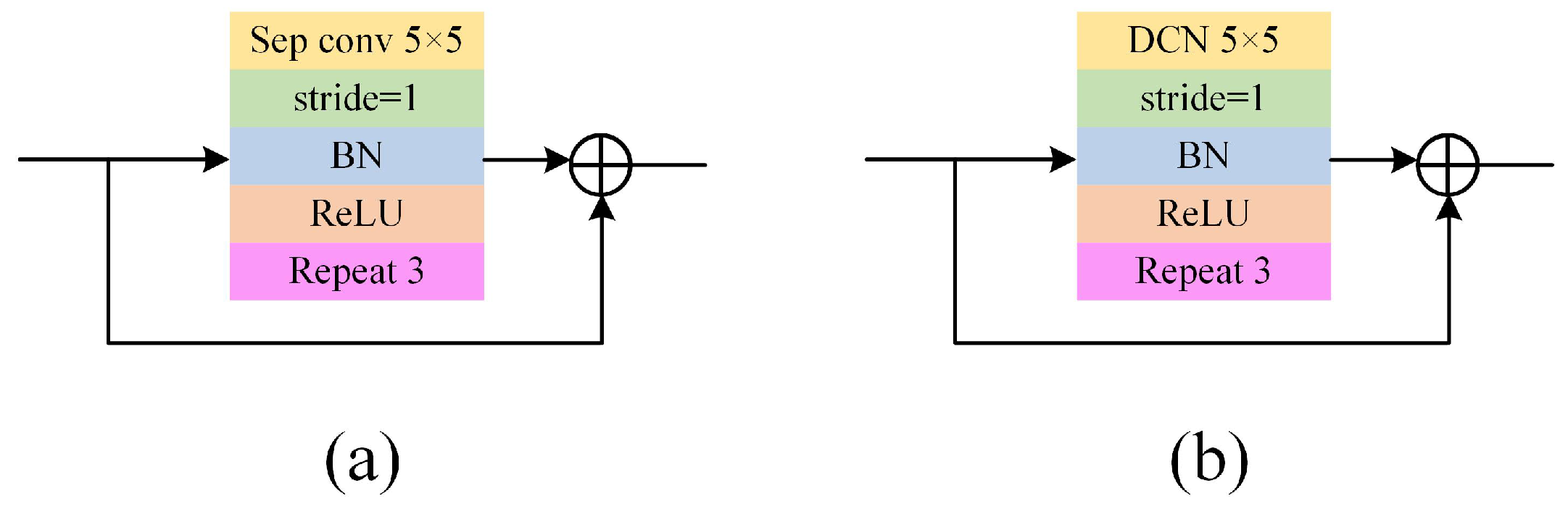
First, the Middle Flow section is structurally reduced by decreasing the number of repeated Block modules from 16 to 8, thereby lowering network depth and computational complexity. Second, in the Exit Flow, the kernel size of the depthwise separable convolution is adjusted from 3 × 3 to 5 × 5, aiming to expand the receptive field and enhance the model’s ability to capture global features. On this basis, the channel count across all convolutional layers in the network is systematically reduced to further control parameter size and improve inference speed. The choice of the channel reduction ratio follows the design principles of lightweight networks. Existing empirical studies have demonstrated that reducing the number of channels to 50–75% of the original can enhance efficiency while minimizing accuracy loss [24,25]. This range is widely recognized as a sweet spot because an over-aggressive reduction (e.g., 50%) may lead to underfitting due to insufficient model capacity, while a conservative reduction fails to achieve significant efficiency gains. Our choice of 75% is positioned at the more accurate end of this validated spectrum, aiming to preserve performance while ensuring lightweight design.

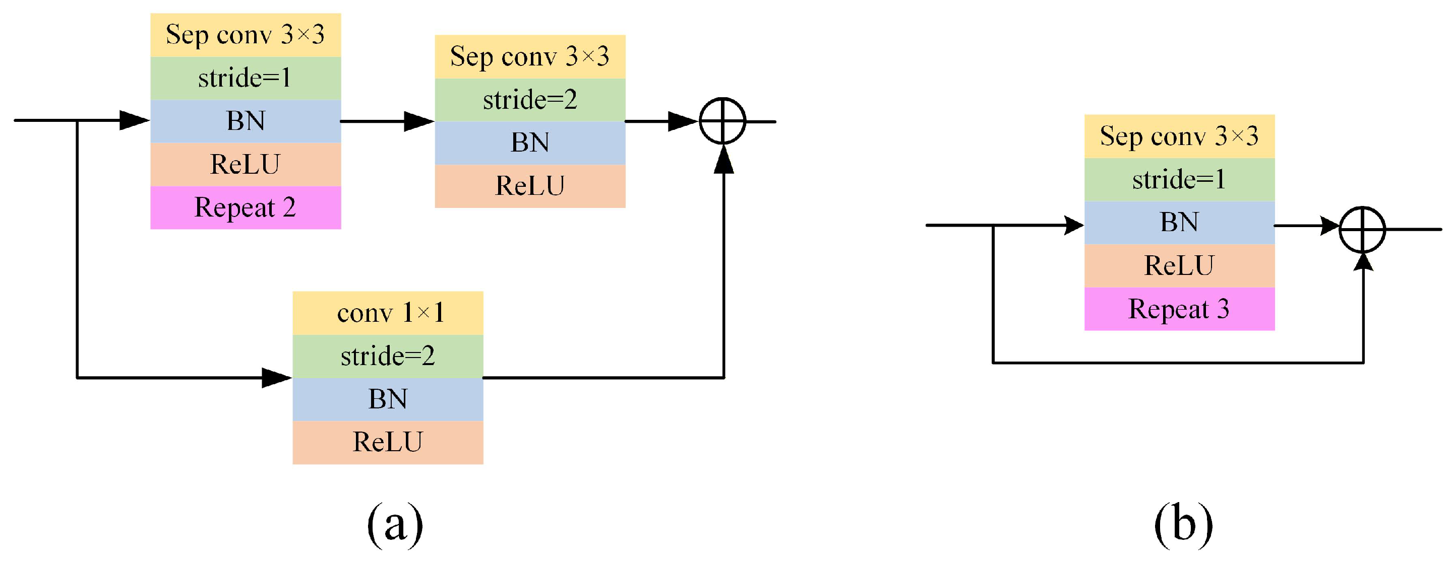
The structures of the Light-Xception backbone network before and after improvement are shown in

Table 1. Architecture of the Baseline Xception Network.

Stage	Operator	Stride	Channels	Layers
Entry Flow	Conv 3 × 3	2	32	1
Entry Flow	Conv 3 × 3	1	64	1
Entry Flow	Block 1	1/2	128	1
Entry Flow	Block 2	1/2	256	1
Entry Flow	Block 3	1/2	728	1
Middle Flow	Block 4–19	1	728	16
Exit Flow	Block 20	1/2	1024	1
Exit Flow	SepConv 3 × 3	1	1536	1
Exit Flow	SepConv 3 × 3	1	1536	1
Exit Flow	SepConv 3 × 3	1	2048	1

and

Table 2. Architecture of the Proposed Light-Xception Network.

Stage	Operator	Stride	Channels	Layers
Entry Flow	Conv 3 × 3	2	24	1
Entry Flow	Conv 3 × 3	1	48	1
Entry Flow	Block 1	1/2	96	1
Entry Flow	Block 2	1/2	192	1
Entry Flow	Block 3	1/2	546	1
Middle Flow	Block 4–11	1	546	8
Exit Flow	Block 12	1/2	768	1
Exit Flow	SepConv 5 × 5	1	1152	1
Exit Flow	SepConv 5 × 5	1	1152	1
Exit Flow	SepConv 5 × 5	1	1536	1

, respectively, with the structure of the core Block module illustrated in Figure 2.

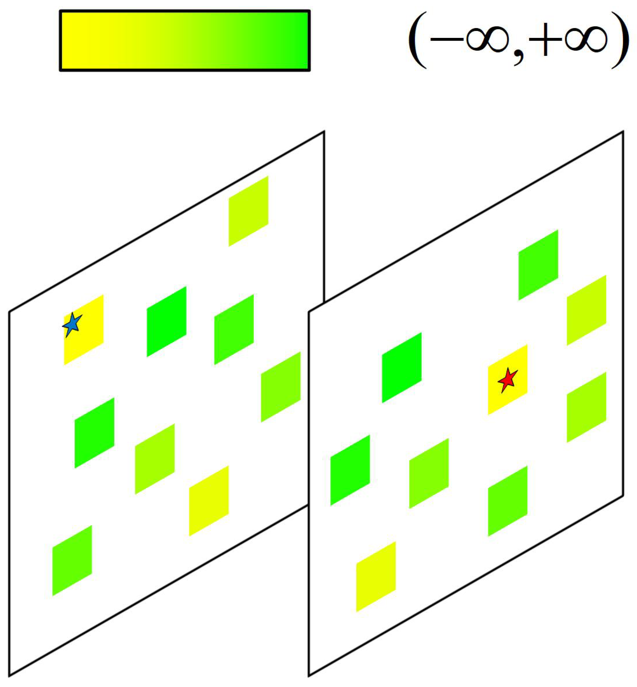
Then, this paper replaces part of the standard convolutional networks with DCNs. The DCN was proposed by Dai et al. [26], and its core idea is to allow the sampling points of the convolution kernel to no longer be confined to fixed grid positions but to dynamically adjust the sampling locations based on the content of the input image. This dynamic characteristic enables it to better adapt to various deformations, scales, and poses of target objects, making it particularly suitable for handling irregular shapes and complex scenes. The DCN used in this paper is DCNv4, which is specifically designed for a wide range of visual applications. Its structure is shown in Figure 3.

DCNv4 removes the softmax normalization operation present in DCNv3, transforming the spatial aggregation weights from a bounded range of [0, 1] to unbounded dynamic weights. This grants it a weight range analogous to conventional convolutions, resulting in more flexible regulatory capability. This modification significantly enhances the operator’s dynamic characteristics and expressive power, thereby achieving faster convergence speed and stronger feature learning ability. The blue and red star symbols in the diagram symbolize the core dynamic mechanisms of the Deformable Convolution (DCN): the blue star represents the dynamically offset sampling locations based on the input content, and the red star represents the dynamically generated attention weights. Together, they enable the model to adaptively focus on key feature regions.Furthermore, DCNv4 allows a single thread to handle multiple consecutive channels within the same group and employs vectorized load instructions to read data from multiple channels at once, greatly reducing redundant memory access and bilinear interpolation calculations. For a DCNv4 operator with G groups and K sampling points, the output y(p) at a position p can be represented by Equation (1):

$$y\left(p\right)={\displaystyle \sum _{g=1}^G}{\displaystyle \sum _{k=1}^K}{w}_g·m_{gk}·x_g\left(p+pk+\Delta p_{gk}\right)$$

(1)

where G represents the total number of aggregation groups, which divides the channel dimension into groups, with each group independently learning offsets, K denotes the total number of sampling points in the convolution kernel, w_g is the static convolution weight for the g-th group, m_gk indicates the unbounded dynamic aggregation weight for the k-th sampling point in the g-th group, x_g is the channel slice of the input feature map corresponding to the g-th group, p represents the spatial position on the current output feature map, p_k is the predefined fixed offset of the k-th sampling point relative to the center point; p_gk denotes the learnable offset for the k-th sampling point in the g-th group.

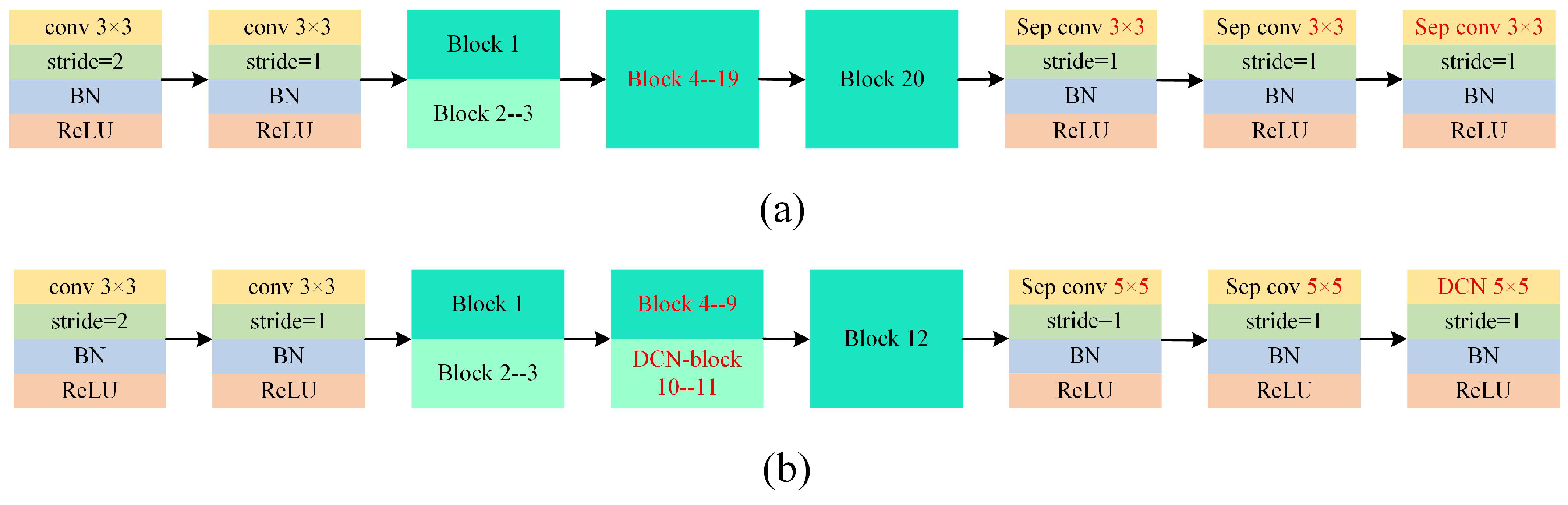
The architecture of Xception network can be divided into three sequential data flows: the Entry Flow, the Middle Flow, and the Exit Flow. The Entry Flow is primarily responsible for extracting general and low-level features from the input image. At this stage, the feature maps have a limited receptive field and relatively simple spatial structures. Therefore, introducing complex deformable convolutions prematurely offers limited benefits for geometric adaptation capability. The Middle Flow captures higher-level semantic information and abstract features, while the Exit Flow represents the final stage of feature extraction, producing the most abstract features that are directly crucial for the classification and boundary determination of cloud clusters. In these two later stages, the complexity of cloud formations—including their varying shapes, scales, and boundaries—places higher demands on the model’s ability to handle geometric transformations. Deformable convolutions address this by introducing learnable offsets, allowing the convolution kernels to adaptively adjust their sampling locations based on the input content, thereby transforming the fixed receptive field into a flexible and variable structure. Consequently, this study adopts a systematic replacement strategy: DCNs are introduced starting from the final layers of each flow and moving toward earlier layers. Specifically, in the Middle Flow, replacements begin from the last block (block 11) and proceed to the previous block (block 10, then block 9, etc.); in the Exit Flow, replacements start from the last SepConv 5 × 5 layer and move to the preceding SepConv 5 × 5 layer. This strategy ensures the model is enhanced with geometric deformation perception precisely at the most critical stages, while avoiding unnecessary computational overhead in the shallower layers, thus achieving an effective balance between performance and efficiency.

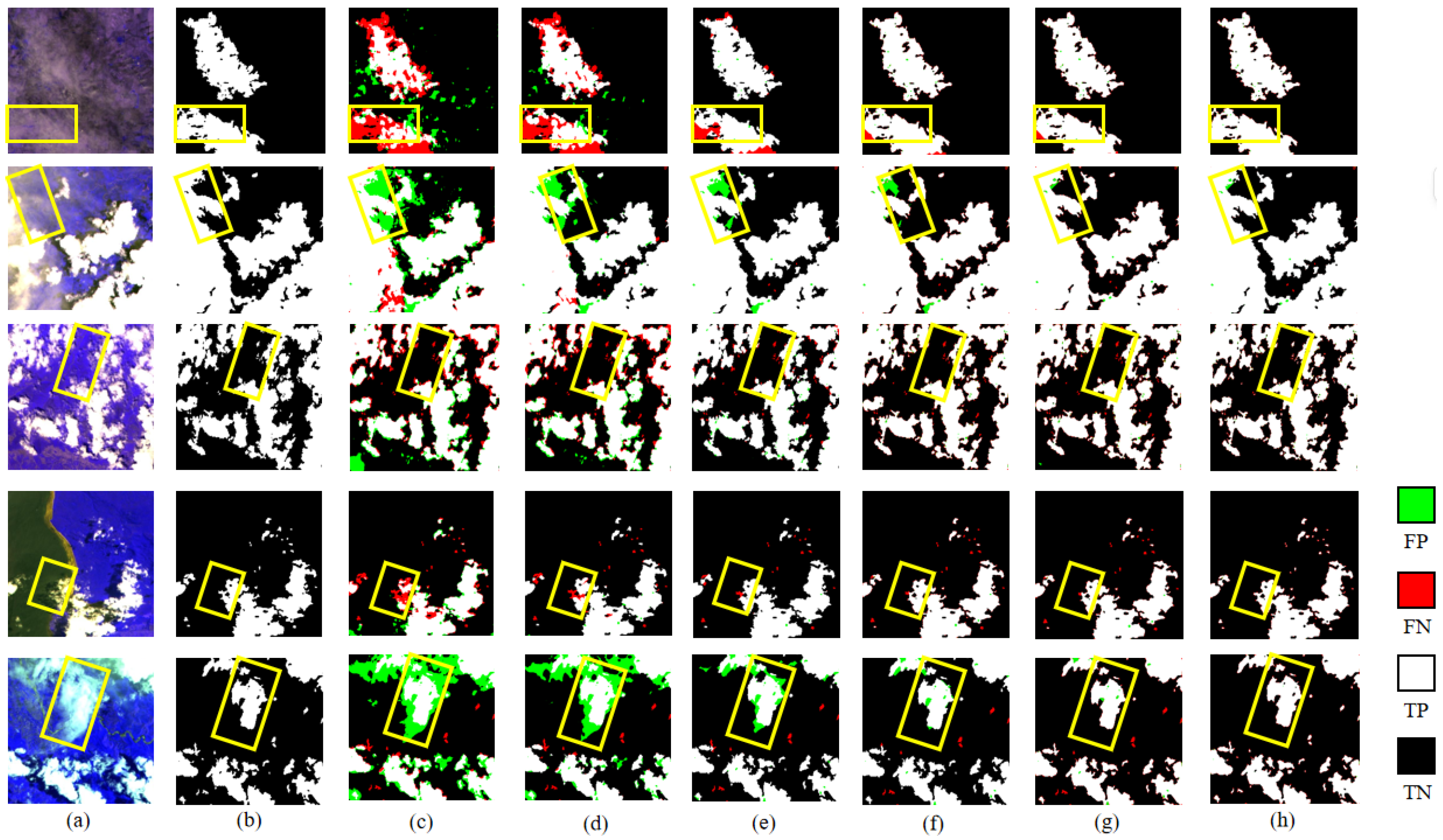
To validate the effectiveness of the proposed scheme, a systematic comparative experiment was designed to investigate the impact of incorporating different numbers of DCNs on the segmentation performance of the model. The experimental results are summarized in

Table 3. Performance comparison of the model after introducing different numbers of DCNs.

Lightweight	Number of DCNs in Middle Flow	Number of DCNs in Exit Flow	MIoU (%)	Training Time (h)
×	0	0	86.57	7.55
✓	0	0	86.46	5.01
	1	0	86.94	6.34
	0	1	87.17	5.71
	1	1	87.88	6.98
	2	1	88.49	8.48
	3	1	88.62	9.86
	3	2	88.70	10.61
	4	2	88.74	13.11
	4	3	88.82	15.66

, where the MIoU serves as the core evaluation metric, measuring the spatial overlap accuracy between the predicted cloud masks and the actual cloud regions. The specific calculation formula for this metric and the detailed experimental settings are provided in Section 4.1.

As shown in Table 3, the lightweight modification reduces the training time by 33.6% without significantly compromising model performance. The introduction of DCNs into both the Middle Flow and the Exit Flow enhances model performance but also increases the training time. Since further additions beyond 2 DCNs in the Middle Flow and 1 DCN in the Exit Flow yield only marginal improvements in performance while still increasing the training duration, this paper adopts the configuration of 2 DCNs in the Middle Flow and 1 DCN in the Exit Flow to balance model performance and training efficiency.

Consequently, the structure of the final backbone feature extraction network, named Light-DCN-Xception, is compared with the original architecture in Figure 4. A comparison of the Block module before and after integrating the DCNs is presented in Figure 5.

2.3. DCM-ASPP

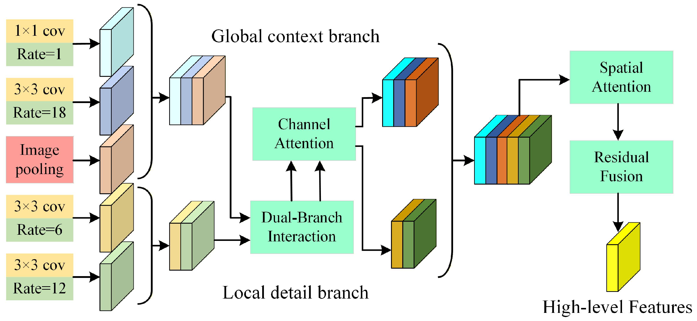
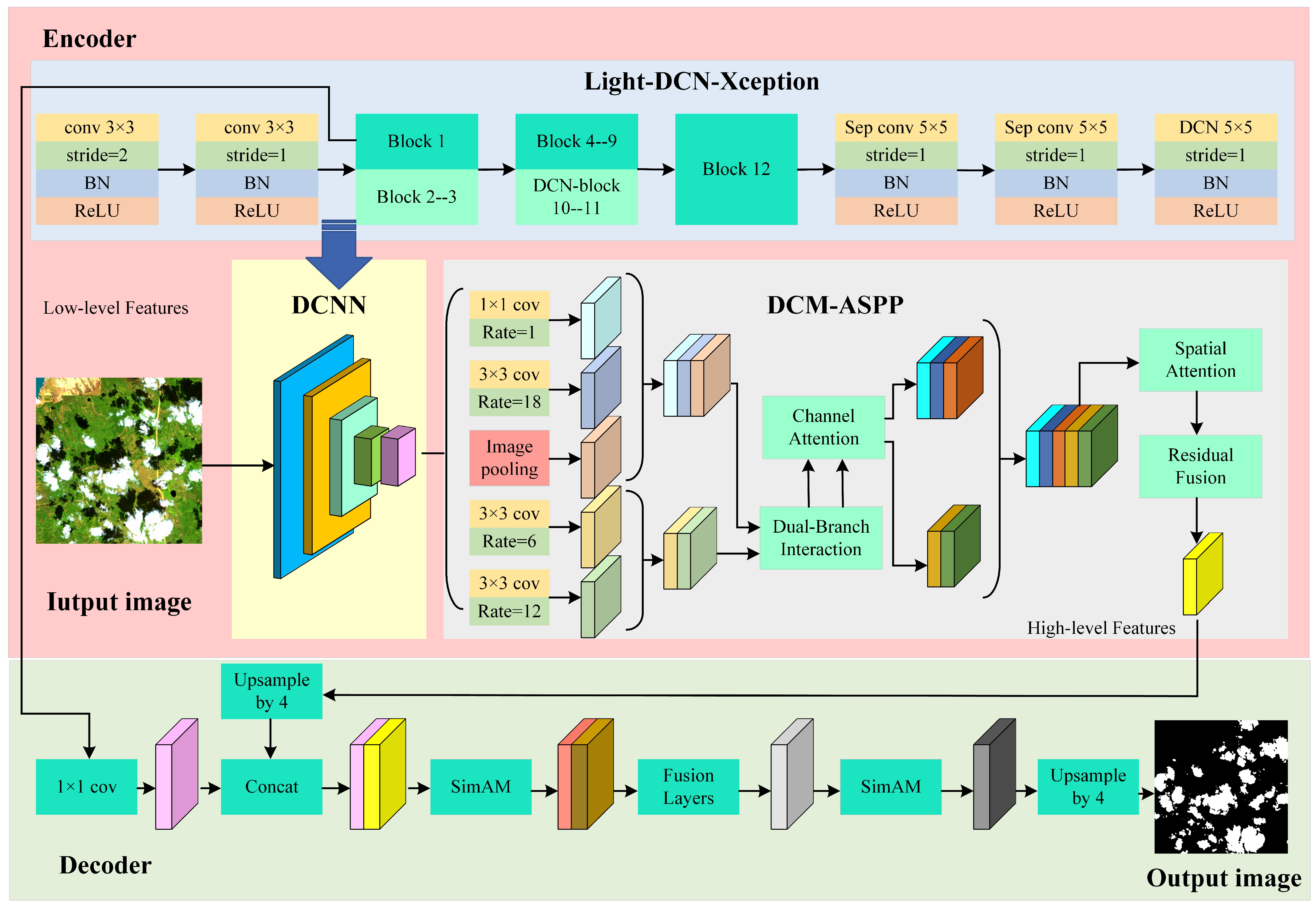
To address the limitations of the DeepLabV3+ model in fully leveraging global contextual information and preserving local details (such as thin cloud edges) when processing clouds with highly variable morphology, this study reconstructs the original Atrous Spatial Pyramid Pooling module by introducing a dual-branch interaction mechanism. The structure of this mechanism is illustrated in Figure 6.

In the proposed ASPP module, the global context branch integrates a 1 × 1 convolution, an atrous convolution with the maximum atrous rate, and image pooling. Their functions are to provide basic contextual information, capture extremely large-scale contextual information, and supply image-level global features, respectively. The local detail branch consists of two atrous convolutions with medium atrous rates. These convolutions possess smaller receptive fields, making them more sensitive to high-frequency details. The two branches first achieve information complementarity through a collaborative mechanism, and then each incorporates a channel attention mechanism to enhance their respective feature representation capabilities. Subsequently, the features output by the two branches are concatenated, and a spatial attention module is introduced to further focus on key spatial regions, thereby improving spatial discrimination of the features. Finally, a residual fusion module is adopted to replace the original simple concatenation followed by 1 × 1 convolution fusion method in the ASPP. The residual connections in this module effectively alleviate the vanishing gradient problem in deep networks, leading to more stable training and more thorough feature fusion, while simultaneously enhancing the characterization of cloud texture features.

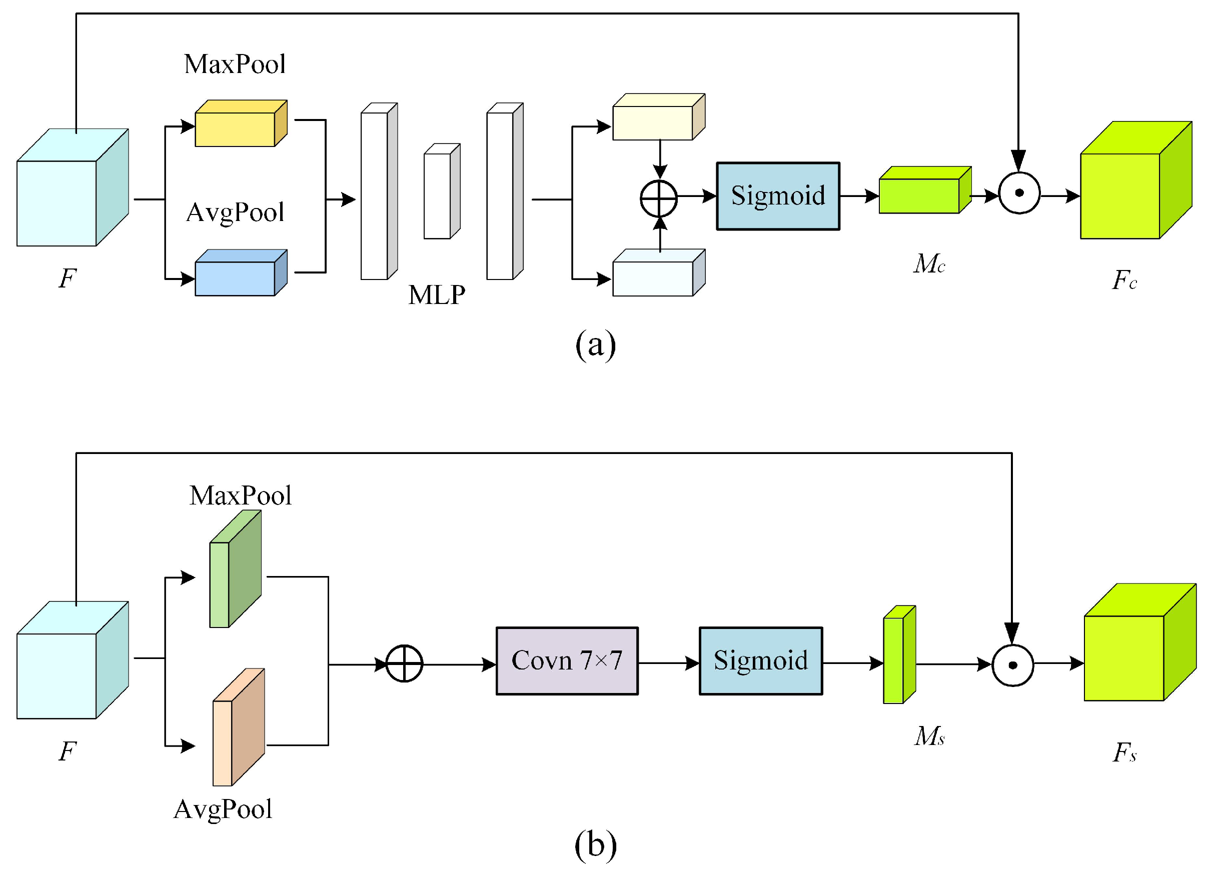
A channel attention module and a spatial attention module are added to the network to improve its ability to capture critical features. The structural diagrams of these modules are presented in Figure 7.

Figure 7a illustrates the structure of the channel attention module. This module utilizes two pooling operations—Global Average Pooling (GAP) and Global Max Pooling (GMP)—to compress the two-dimensional features (H × W) of each channel into a single scalar value. The GAP operation captures the overall contextual information of the feature map, while the GMP operation highlights the most salient features. Their complementary nature provides a more comprehensive channel descriptor. The corresponding formula is as follows:

$$F_{avg}={\displaystyle \frac{1}{H\times W}}{\displaystyle \sum _{i=1}^H}{\displaystyle \sum _{j=1}^W}F\left(i,j\right)$$

(2)

$$F_{max}=\underset{i=1:H,j=1:W}{\max }F(i,j)$$

(3)

where F represents the input feature matrix, F_avg is the result of the Global Average Pooling operation, H and W are the height and width of the feature matrix, F_max is the result of the Global Max Pooling operation.

Subsequently, the results of these two pooling operations are passed through a shared two-layer neural network. The first layer is a bottleneck layer, which reduces the number of channels to C/r, where r is the reduction ratio, serving to decrease computational complexity and introduce non-linearity. The r is set to 16. This value, consistent with practices in SENet and CBAM, offers a balanced trade-off between model capacity (risking overfitting with small datasets at lower r) and parameter efficiency (risking underfitting with higher r). The second layer restores the number of channels to C. The outputs from the two Multilayer Perceptrons(MLPs) are summed and then passed through a Sigmoid function to obtain the channel attention weight vector M_c. Finally, these weights are multiplied channel-wise with the original input feature map. The expression is as follows:

$$M_c=\sigma \{\mathrm{MLP}\left(F_{avg}\right)+\mathrm{MLP}\left(F_{max}\right))$$

(4)

$$F_c=M_c\odot F$$

(5)

where $\sigma$ denotes the Sigmoid function, where $\sigma$(x) = 1/(1 + e^−x), represents element-wise multiplication, F_c denotes the output feature matrix of the channel attention module.

Figure 7b illustrates the structure of the spatial attention module. The process begins by applying both average pooling and max pooling along the channel dimension of the input feature map, generating two feature maps of size H × W × 1. The average pooling operation retains overall background information, while max pooling highlights the most salient features. These two resulting feature maps are then concatenated along the channel dimension, forming a combined feature map with two channels. This two-channel feature map is subsequently processed by a convolutional operation, which fuses the two channels into a single channel, thereby capturing the relationships between different spatial locations. The output of this convolution is passed through a Sigmoid function to produce the spatial attention weight map, denoted as Ms. Finally, this weight map is multiplied with the input feature map element-wise. The corresponding expression is as follows:

$$F_{avg}={\displaystyle \frac{1}{C}}{\displaystyle \sum _{k=1}^C}{F}_k$$

(6)

$$F_{max}=\underset{k=1:C}{\max }{F}_k$$

(7)

$$M_s=\sigma \left(f^{7\times 7}\left(\left[F_{avg}·F_{max}\right]\right)\right)$$

(8)

$$F_s=M_s\odot F$$

(9)

where C denotes the number of channels, F_s represents the output feature matrix of the channel attention module, f ^7×7 denotes a convolutional operation with a 7 × 7 kernel.

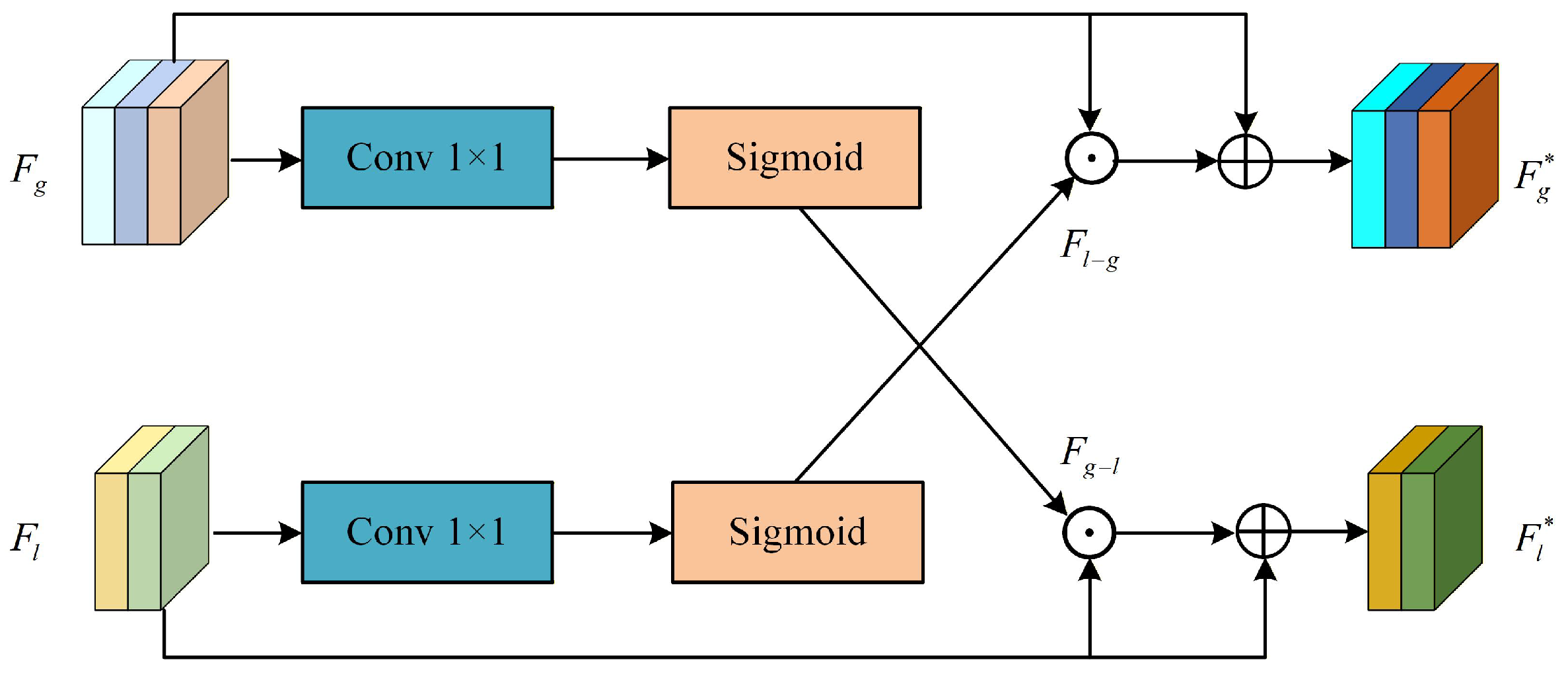
The Dual-Branch Collaborative Module is the core of this mechanism. Its structure is illustrated in Figure 8. The global context branch serves as an attention blueprint, guiding the detail branch on which edges and textures of specific regions to focus on. This effectively suppresses interference from background noise, making detail extraction more purposeful. The local detail branch can, in turn, supplement or correct the global context. It provides a bottom-up signal that enhances the model’s sensitivity to small targets and anomalous areas. The expression is as follows:

$$f_{l-g}=\sigma \left(f^{1\times 1}\left(F_g\right)\right)\odot F_l$$

(10)

$${\displaystyle F_g^{\ast }}=F_g+F_{l-g}$$

(11)

$$f_{g-l}=\sigma \left(f^{1\times 1}\left(F_l\right)\right)\odot F_g$$

(12)

$${\displaystyle F_l^{\ast }}=F_l+F_{g-l}$$

(13)

where F_g represents the feature matrix of the global context branch, F_l−g representsthe guidance from the local detail branch to the global context branch, F_g^* represents the feature matrix of the global context branch after interaction, F_l represents the feature matrix of the local detail branch, F_g−l represents the guidance from the global context branch to the local detail branch, F_l^* represents the feature matrix of the local detail branch after interaction, f^1×1 denotes a convolutional operation with a 1 × 1 kernel.

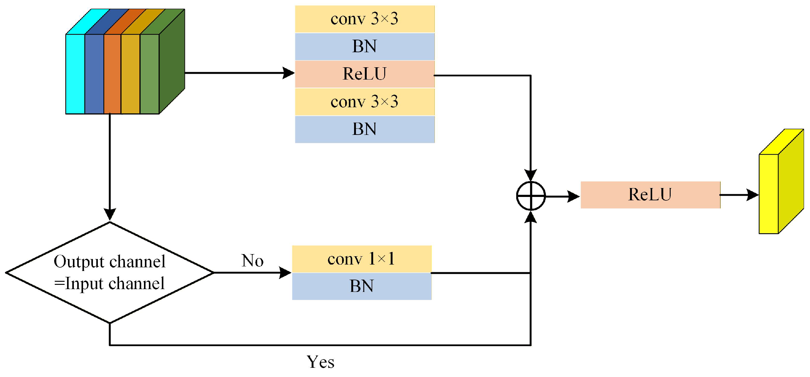
Finally, the two branches are fused using a residual fusion module, the structure of which is illustrated in Figure 9. This module primarily consists of three components. The main fusion path serves as the core computational part of the module, comprising two 3 × 3 convolutional layers, each followed by Batch Normalization. The purpose of this path is to learn complex, non-linear feature transformations from the input to the output. The shortcut connection path is the essence of residual learning. If the input and output have the same number of channels, an identity mapping is used directly. If the number of channels differs, a 1 × 1 convolution is employed to align the channel dimensions. This path ensures that the input features can be propagated forward without loss. The output of the main path and the output of the shortcut connection are combined using element-wise addition. Finally, the result is passed through a ReLU activation function. The expression is as follows:

$$\mathrm{BN}\left(x\right)=\gamma {\displaystyle \frac{x-\mu }{{\sqrt{\sigma }}^2+\epsilon }}+\beta$$

(14)

$$F_{\mathrm{main}}=\mathrm{BN}\left(f^{3\times 3}\left(\mathrm{ReLU}\left(\mathrm{BN}\left(f^{3\times 3}\left(x\right)\right)\right)\right)\right)$$

(15)

$$F_{\mathrm{shortcut}}=\left\{\begin{array}{cc}x& \mathrm{Output}\mathrm{Channel}=\mathrm{Input}\mathrm{Channel}\hfill \\ BN\left(f^{1\times 1}\left(x\right)\right)& \mathrm{Output}\mathrm{Channel}\ne \mathrm{Input}\mathrm{Channel}\hfill \end{array}\right.$$

(16)

$$F_{\mathrm{output}}=\mathrm{ReLU}\left(F_{\mathrm{main}}+F_{\mathrm{shortcut}}\right)$$

(17)

where BN denotes the Batch Normalization layer of the convolutional neural network, x is the input feature, $\mu$ is the mean of the batch, $\sigma$² is the variance of the batch, $\epsilon$ is a small constant to prevent division by zero, $\gamma$ is the learnable scaling parameter, $\beta$ is the learnable shift parameter, F_main represents the output feature matrix of the main fusion path, F_shortcut represents the output feature matrix of the shortcut connection path, and F_output is the final output feature matrix, ReLU stands for Rectified Linear Unit, expressed as ReLU(x) = max(0, x), and f ^3×3 denotes a convolutional operation with a 3 × 3 kernel.

2.4. SimAM-Decoder

Although the DeepLabV3+ model has achieved remarkable results in semantic segmentation tasks through its encoder–decoder architecture, its decoder treats all feature channels and spatial locations equally when integrating high-level and low-level features. This approach may fail to adequately emphasize texture and boundary details critical for cloud detection, leading to insufficient precision in segmenting edges of irregular targets such as thin clouds and fragmented clouds. To enhance the model’s ability to focus on key features while avoiding a significant increase in computational complexity and training time, this paper integrates a parameter-free attention module named SimAM into the decoder.

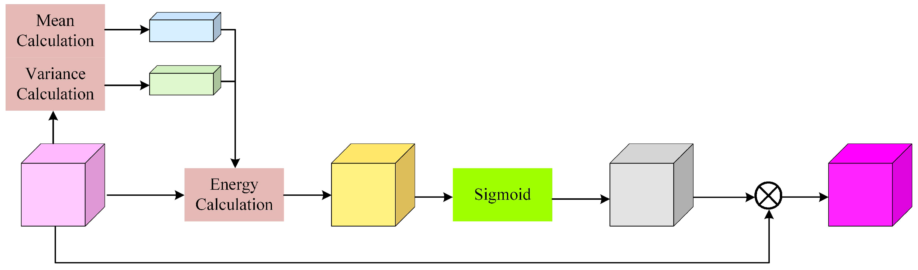
SimAM is an attention mechanism based on the spatial suppression theory in neuroscience [27]. This mechanism employs an energy function to evaluate the importance of each neuron in the feature map: neurons with lower energy exhibit more distinct responses compared to their neighbors and are thus considered more critical in visual tasks. In remote sensing cloud detection, the edges of thin clouds, fragmented cloud areas, and their boundaries with the underlying surface represent such key regions with discriminative features, where pixels possess subtle yet crucial differences in spectral and texture characteristics from the surrounding background. SimAM can automatically identify and enhance these feature responses through the energy function, thereby effectively improving the model’s ability to capture fine details. Furthermore, the module requires no learnable parameters and computes 3D attention weights across both channel and spatial dimensions, achieving efficient feature enhancement and suppression of redundant information. Its structure is illustrated in Figure 10.

The core of SimAM is a carefully designed energy function that evaluates the importance of each neuron. The attention weight for a neuron is then normalized using a Sigmoid function. Finally, the enhanced features are obtained through element-wise multiplication. The expression is as follows:

$$\mu ={\displaystyle \frac{1}{H\times W}}{\displaystyle \sum _{i=1}^H}{\displaystyle \sum _{j=1}^W}{X}_{i,j}$$

(18)

$${\sigma }^2={\displaystyle \frac{1}{H\times W-1}}{\displaystyle \sum _{i=1}^H}{\displaystyle \sum _{j=1}^W}{\left(X_{i,j}-\mu \right)}^2$$

(19)

$$E_{i,j}={\displaystyle \frac{{\left(X_{i,j}-\mu \right)}^2}{4\left({\sigma }^2+\epsilon \right)}}+0.5$$

(20)

$$X^{\ast }=X\times \mathrm{Sigmoid}\left(E\right)$$

(21)

where E represents the computed energy value, X is the input feature, and $\epsilon$ is a small constant to prevent division by zero.

This paper designs an improved decoder integrated with SimAM, whose structure is shown in Figure 11. First, the low-level feature maps obtained from the backbone extraction network of the encoder undergo a 1 × 1 convolution for channel dimensionality reduction. This step aims to decrease computational load and balance the contribution from high-level features. The high-level features are then upsampled and concatenated with the low-level features. The SimAM attention mechanism is applied to both feature sets separately. This process enhances the decoder’s sensitivity to crucial spatial details and semantic information, particularly in edge regions where the contrast between clouds and the background is low. The reinforced features are subsequently smoothed and fused through two 3 × 3 convolutional layers. Following this, the SimAM module is applied again to the fused features for final refinement, further strengthening the feature expression in target regions and thereby improving the boundary clarity of the segmentation mask.

2.5. Loss Function

In binary semantic segmentation, integrating the advantages of Binary Cross-Entropy (BCE) Loss and Dice Loss into a composite function is a widely adopted strategy. The L_BCE quantifies the pixel-wise dissimilarity between predictions and ground truth labels. In contrast, the L_Dice, derived from the Dice coefficient, evaluates the spatial overlap between predicted and actual regions, making it particularly effective for segmentation tasks by emphasizing boundary alignment. The definitions of these two loss components are given below:

$$L_{\mathrm{BCE}}=-{\displaystyle \frac{1}{N}}{\displaystyle \sum _{i=1}^N}\left[y_{i}log\left({\lambda }_i\right)+(1-y_i)log(1-{\lambda }_i)\right]$$

(22)

$$L_{\mathrm{Dice}}=1-{\displaystyle \frac{2{\displaystyle {\sum }_{i=1}^N}{\lambda }_i{y}_i}{{\displaystyle {\sum }_{i=1}^N}{\displaystyle {\lambda }_i^2}+{\displaystyle {\sum }_{i=1}^N}{\displaystyle y_i^2}}}$$

(23)

where N represents the total number of samples, y_i denotes the ground truth label for the i-th sample, $\lambda$_i indicates the predicted probability of the i-th sample belonging to the positive class. The composite loss function is formulated as a weighted sum of the two components:

$$L_{\mathrm{loss}}=L_{\mathrm{BCE}}+\rho L_{\mathrm{Dice}}$$

(24)

where the hyperparameter $\rho$ is introduced to balance the contribution of the L_BCE relative to the L_Dice. The value of $\rho$ = 1.2 was selected to place a stronger emphasis on the Dice loss. This is a common strategy in semantic segmentation tasks characterized by class imbalance, such as cloud detection, where the foreground (clouds) often occupies a smaller area than the background. The Dice loss directly optimizes for spatial overlap, which is critical for precise boundary delineation. A value greater than 1 (like 1.2) helps mitigate the tendency of the cross-entropy loss to be dominated by the majority background class, thereby improving the segmentation accuracy of cloud pixels [28,29].

3. Dataset Set

To comprehensively evaluate the performance of the proposed method, this study employs two datasets for experimentation.

The Landsat-8 Cloud Cover Assessment Validation Data (L8Biome dataset) [13] provides a systematically collected benchmark spanning eight representative natural biomes. This diversity ensures evaluation under various land cover conditions that present distinct cloud detection challenges. The dataset comprises 96 high-resolution multispectral images (approximately 7500 × 7800 pixels each) acquired by the Operational Land Imager (OLI) and Thermal Infrared Sensor (TIRS). Each image contains eight spectral bands covering visible, near-infrared (NIR), short-wave infrared (SWIR), and thermal infrared ranges. Following the USGS standard cloud detection synthesis scheme [30], the paper generates false-color images using a specific band combination: Blue, NIR, and SWIR. This combination is scientifically established to enhance contrast between cloud features and underlying surfaces, particularly for thin cloud detection against varied backgrounds. To accommodate computational constraints while preserving sufficient spatial context, original images are divided into 512 × 512 pixel patches using a sliding window approach with 20% overlap. This patch size represents an optimal balance between GPU memory limitations and contextual information requirements for accurate cloud boundary detection. The dataset is randomly partitioned into training, validation, and test sets at 70:15:15 ratio. For label consistency, thin cloud is redefined as cloud, and cloud shadow as clear sky.

The GF-1 Cloud and Cloud Shadow Cover Validation Data (referred to as the GF-1 dataset) [31] includes 108 wide-scene Level-2A original images acquired by the Gaofen-1 satellite. Each original image has a spatial resolution of approximately 15,700 × 16,200 pixels and consists of four spectral channels covering the visible and near-infrared bands. In accordance with the USGS standard cloud detection methodology, false-color images are synthesized using an optimized band combination adapted to GF-1’s sensor characteristics: the blue, green, and near-infrared bands. This adaptation maintains the core USGS principle of maximizing cloud-background contrast while respecting the specific spectral capabilities of the GF-1 sensor, which lacks the short-wave infrared (SWIR) bands available in Landsat-8. All original images are cropped into 512 × 512 pixel patches using a sliding window approach from left to right and top to bottom. These patches are then randomly divided into training, validation, and test sets in a 70:15:15 ratio. The cloud shadow category is redefined as clear sky to maintain labeling consistency across datasets.

The final experimental results are summarized in

Table 4. Dataset Summary.

Dataset Name	Pixel	Train	Val	Test
Landsat-8	512 × 512	4004	858	858
GF-1	512 × 512	3780	810	810

.

4. Experimental Results and Analysis

4.1. Experimental Setup and Evaluation Metrics

The experiments in this study were implemented using Python 3.8 as the programming language and PyTorch 1.8.1 as the deep learning framework. The hardware platform consisted of a Linux system with an Intel(R) Core(TM) i5-12400 CPU @ 2.50 GHz and an NVIDIA RTX 3080 GPU. The training hyperparameters were set as follows: batch size = 8, number of epochs = 150, and learning rate = 0.05, weight decay = 0.0005.

To quantitatively evaluate the accuracy of cloud detection, this paper employs Overall Accuracy (OA), Precision (P), Recall (R), F1-score (F1), Mean Intersection over Union (MIoU), and Kappa coefficient (Ka) as evaluation metrics. The values of these metrics generally range between 0 and 1, with higher values indicating better performance. Their definitions are provided below:

$$\mathrm{OA}={\displaystyle \frac{\mathit{TP}+TN}{\mathit{TP}+FP+TN+FN}}$$

(25)

$$\mathrm{P}={\displaystyle \frac{\mathit{TP}}{\mathit{TP}+FP}}$$

(26)

$$\mathrm{R}={\displaystyle \frac{\mathit{TP}}{\mathit{TP}+FN}}$$

(27)

$$\mathrm{F}1={\displaystyle \frac{2\times \mathrm{P}\times \mathrm{R}}{\mathrm{P}+\mathrm{R}}}$$

(28)

$$\mathrm{MIoU}={\displaystyle \frac{1}{2}}\left({\displaystyle \frac{\mathit{TP}}{\mathit{TP}+FN+\mathit{FP}}}+{\displaystyle \frac{\mathit{TN}}{\mathit{TN}+FN+\mathit{FP}}}\right)$$

(29)

$$p_e={\displaystyle \frac{P(\mathit{TP}+FP)+N(\mathit{TN}+FN)}{{(\mathit{P}+N)}^2}}$$

(30)

$$\mathrm{Ka}={\displaystyle \frac{p_0-p_e}{1-p_e}}$$

(31)

where TP, TN, FP, and FN are the total number of true positive, true negative, false positive, and false-negative pixels. P and N represent the total number of cloud and clear-sky pixels in the ground truth labels, respectively. The overall accuracy is denoted as p₀ = OA.

To evaluate the computational efficiency of the cloud detection method, this paper uses the number of model parameters (Params) and the floating-point operations per second (FLOPs) as efficiency metrics.

Aiming to address the instability issues caused by the second-order optimization mechanism of DCNs during the initial training phase [32], a progressive DCN intensity enhancement strategy is proposed. Inspired by the human cognitive process of learning from simple patterns to complex concepts, this strategy restricts the activation scope of DCNs in the early training stages, allowing the network to prioritize learning basic semantic features. As the number of training epochs increases, the activation scope of DCNs is gradually expanded to smoothly introduce deformable modeling capabilities. This mechanism not only enhances training stability but also enables the network to adapt to geometric transformations of varying complexity in stages, ultimately improving feature learning performance. The performance comparison of models using different progressive enhancement strategies is shown in

Table 5. Performance comparison of models trained with different progressive strategies.

Progressive Strategies	Epoch A	Epoch B	Epoch C	MIoU (%)	Training Time (h)
×	0	0	0	91.67	9.07
✓	21	41	31	91.95	8.36
	31	61	46	92.28	8.01
	41	81	61	92.61	7.66
	51	101	76	92.03	7.31
	61	121	91	91.21	6.95

, where Epoch A, B, and C represent the starting training epochs for enabling DCNs in Middle Flow block11, Middle Flow block10, and Exit Flow, respectively.

The enhancement timing is selected based on the experimental configuration in Table 5 that achieved the highest MIoU of 92.61%. The results indicate that introducing DCNs in phases—specifically at epochs 41, 81, and 61 during the mid-stage of model training—achieves an optimal balance between performance and efficiency. If activated too early, the model’s foundational feature learning is insufficient, leading to limited performance gains. Conversely, if activated too late, the model lacks sufficient training iterations to fully learn deformable representations, resulting in a performance of 91.21% that is even lower than the 91.67% baseline without this strategy. The peak performance achieved with our schedule (epochs 41, 81, 61) validates this curriculum learning approach, demonstrating that a phased introduction of complexity leads to more effective and stable learning than either premature or delayed introduction. Thus, the results in Table 5 are not merely empirical but provide empirical evidence for a principled training strategy. This progressive strategy not only identifies the performance peak but also significantly reduces the training time from 9.07 h to 7.66 h, thereby effectively improving training efficiency.

4.2. Ablation Study of Key Components

To systematically analyze the functional characteristics of each key component in DDS-DeeplabV3+ and quantify their contribution to the overall model performance, this paper conducts a comprehensive ablative study on the Landsat-8 and GF-1 dataset. The study employs a progressive framework design, starting from a baseline model and incrementally integrating our proposed modules to construct various experimental variants. To ensure a fair comparison, all experiments adopt the same hyperparameter settings, and all variants containing DCNs are trained using the progressive strategy. The results on the Landsat-8 and GF-1 datasets are summarized in

Table 6. Ablation for different modules on Landsat-8 dataset (in%).

Method	Light-DCN-Xception	DCM-ASPP	SimAM	OA	F1	MIoU
Deeplabv3+				93.10	91.25	86.57
Scheme 1	✓			94.63	93.26	89.44
Scheme 2		✓		93.78	91.87	88.56
Scheme 3			✓	93.54	91.64	88.06
Scheme 4	✓	✓		95.49	94.27	91.18
DDS-Deeplabv3+	✓	✓	✓	96.35	95.30	92.61

and

Table 7. Ablation for different modules on GF-1 dataset (in%).

Method	Light-DCN-Xception	DCM-ASPP	SimAM	OA	F1	MIoU
Deeplabv3+				94.40	93.10	88.39
Scheme 1	✓			95.78	95.03	91.25
Scheme 2		✓		95.07	93.68	90.37
Scheme 3			✓	94.92	91.64	89.87
Scheme 4	✓	✓		96.41	95.33	92.84
DDS-Deeplabv3+	✓	✓	✓	97.07	96.25	94.04

, respectively.

As shown in Table 6 and Table 7, after introducing the Light-DCN-Xception backbone, all evaluation metrics show significant improvement. Specifically, the MIoU increases by 2.87% on the Landsat-8 dataset and 2.86% on the GF-1 dataset. When the DCM-ASPP module is adopted, the model performance is further enhanced, with MIoU rising by 1.99% on Landsat-8 and 1.94% on GF-1. Integrating the SimAM attention module also brings a consistent gain, improving MIoU by 1.49% and 1.38% on the two datasets, respectively. These results confirm that each proposed improvement effectively strengthens the performance of the model. When all three modules are combined, the model achieves a substantial synergistic gain, ultimately boosting MIoU by 6.04% on Landsat-8 and 5.65% on GF-1.

4.3. Comparison Test

This study compares the cloud detection performance of the proposed method with current mainstream approaches on the Landsat-8 and GF-1 test sets. The compared methods include widely-used semantic segmentation models for natural scenes as well as cloud detection algorithms specifically designed for remote sensing imagery. The natural-scene semantic segmentation models comprise FCN [33], PSPNet [34], U-Net [16], SegNet [35], and DeepLabv3+ [36]. The remote-sensing cloud detection models include CloudU-Net [37], CDNet [38], HR-Cloud-Net [39], Cloud-Adapter [40], and MSCloudCAM [41].

To ensure a fair comparison, all experiments adopt the same set of hyperparameters. The experimental results of different models on the Landsat-8 and GF-1 test sets are presented in

Table 8. Comparison Test of the Landsat-8 Dataset (in%) (%).

Method	OA	P	R	F1	MIoU	Ka
FCN	93.20	90.55	92.71	91.62	86.86	85.90
PSPNet	91.08	87.57	90.60	89.06	83.14	81.53
U-Net	90.63	86.59	90.54	88.52	82.37	80.61
SegNet	92.72	89.87	92.93	91.03	86.00	84.91
Deeplabv3+	93.10	90.92	91.59	91.25	86.57	85.56
CloudU-Net	94.72	92.73	94.22	93.47	89.63	89.04
CDNet	95.34	94.31	93.79	94.05	90.69	90.22
HR-Cloud-Net	95.78	95.90	93.25	94.56	91.50	91.11
Cloud-Adapter	96.18	96.42	93.76	95.07	92.28	91.95
MSCloudCAM	96.25	95.47	94.95	95.21	92.44	92.12
DDS-Deeplabv3+	96.35	96.44	94.19	95.30	92.61	92.31

and

Table 9. Comparison Test of the GF-1 Dataset (in%).

Method	OA	P	R	F1	MIoU	Ka
FCN	94.60	93.75	92.71	93.23	89.36	88.74
PSPNet	91.78	89.08	90.60	89.83	84.32	82.93
U-Net	91.56	88.56	90.54	89.54	83.92	82.47
SegNet	93.65	91.00	93.39	92.18	87.68	86.84
Deeplabv3+	94.40	91.91	94.33	93.10	89.05	88.39
CloudU-Net	95.02	93.06	94.45	93.75	90.14	89.61
CDNet	95.44	94.07	94.58	94.32	90.95	90.51
HR-Cloud-Net	96.43	96.47	94.36	95.40	92.76	92.48
Cloud-Adapter	96.90	96.59	95.48	96.04	93.71	93.50
MSCloudCAM	97.03	96.58	95.83	96.20	93.96	93.76
DDS-Deeplabv3+	97.07	96.60	95.51	96.25	94.04	93.85

, respectively.

As shown in Table 8, the U-Net model yields the poorest performance among all compared methods. This observation indicates that cloud detection models specifically designed for remote sensing imagery generally outperform generic semantic segmentation models developed for natural scenes. The proposed DDS-DeeplabV3+ model achieves the highest scores on the Landsat-8 test set across five key metrics: Overall Accuracy (OA), Precision (P), F1-Score, Mean Intersection over Union (MIoU), and Kappa coefficient (Ka). Although its Recall (R) is slightly lower than that of MSCloudCAM, the superior performance in the other comprehensive metrics fully demonstrates the overall excellence of the proposed model. Specifically, an MIoU of 92.61% on Landsat-8 confirms the strong segmentation capability of our model on this dataset.

Results presented in Table 9 similarly show that U-Net performs the worst on the GF-1 dataset, further validating that specialized remote sensing cloud detection models have superior performance compared to general-purpose semantic segmentation models. On the GF-1 test set, the Recall (R) of DDS-DeeplabV3+ is marginally lower than that of MSCloudCAM. However, it outperforms MSCloudCAM in the other five metrics (OA, P, F1-Score, MIoU, and Ka). Furthermore, DDS-DeeplabV3+ surpasses all other models except MSCloudCAM across all six metrics, robustly affirming its comprehensive superiority. The MIoU of 94.04% achieved on GF-1 further attests to the powerful segmentation ability of the model on this dataset. Additionally, it is noteworthy that the performance metrics of almost all models on the GF-1 dataset are higher than those on the Landsat-8 dataset. This phenomenon is likely attributable to the higher spatial resolution of GF-1 satellite imagery, which provides clearer details and boundaries of ground objects, thereby facilitating more accurate detection.

The comparative experiments conducted on two distinct datasets and against multiple advanced models demonstrate the superiority of the proposed DDS-DeeplabV3+ model and its good generalization capability.

To compare the computational efficiency of different models, this study conducts a quantitative evaluation from three dimensions: the number of parameters (Params), floating-point operations per second (FLOPs), and inference time. All tests are performed on 600 test images based on a uniform input size of 512 × 512 pixels. The results are shown in

Table 10. Comparison of model complexity and efficiency (%).

Method	Params (M)	FLOPs (G)	Test Time (s)
FCN	134.1	76.8	89.30
PSPNet	26.4	10.1	43.07
U-Net	31.2	176.2	74.96
SegNet	14.7	40.5	38.38
Deeplabv3+	52.2	82.9	60.31
CloudU-Net	135.2	138.9	68.06
CDNet	12.3	55.4	77.73
HR-Cloud-Net	32.1	45.87	56.12
Cloud-Adapter	1.82	10.2	13.28
MSCloudCAM	38.98	47.44	25.01
DDS-Deeplabv3+	39.27	20.09	55.59

.

As shown by the computational results in Table 10, the Cloud-Adapter model achieves extreme computational efficiency while maintaining relatively high model performance, with its number of parameters, floating-point operations (FLOPs), and inference time significantly lower than those of other compared models. The DDS-DeeplabV3+ model proposed in this paper also demonstrates excellent computational efficiency while maintaining leading accuracy: both its parameter count and FLOPs are lower than those of most compared models, and its inference time is shorter than that of the majority of similar algorithms. This indicates that the model successfully balances accuracy with efficiency, thus performing excellently even in resource-constrained environments.

4.4. Visualization Analysis

To more intuitively demonstrate the superior performance of the DDS-DeeplabV3+ model, the detection results of six models (U-Net, Deeplabv3+, CloudU-Net, Cloud-Adapter, MSCloudCAM, and DDS-DeeplabV3+) on the Landsat-8 and GF-1 test sets were selected for visualization to compare their cloud detection capabilities. The results on the Landsat-8 test sets are shown in Figure 12. The yellow frames are used to highlight areas in the visualization results where the performance differences between models are more evident.

Figure 12 demonstrates that the proposed model exhibits high performance in detecting thin and broken clouds, significantly reducing the missed detection rate. Furthermore, while most models tend to misclassify bright ground surfaces as clouds, our model achieves accurate detection and segmentation, validating its strong capability in extracting complex spatial features of cloud formations. Additionally, the segmented edges are smooth and refined, closely aligning with the ground truth labels.

The results on the GF-1 test sets are shown in Figure 13. The yellow frames are used to highlight areas in the visualization results where the performance differences between models are more evident. As shown in Figure 13, in the first image, the unclear boundary between cloud and background leads to substantial false positives and false negatives in several models, whereas the proposed model accurately detects and segments the cloud with only minor errors at the edges. In the second image, affected by solar irradiation, most models produce false positives within the boxed area, while the proposed model correctly identifies the cloud-free region. This is a formal and common way to denote possession or attribution in academic writing. In the fourth image, the cloud within the box is faint, and some models fail to detect it; the accurate segmentation by the proposed model demonstrates its capability in detecting thin clouds. The fifth image shows that the proposed model can still precisely distinguish clouds from surface information even when cloud boundaries are mixed with ground features.

Based on the above visual comparison, the DDS-DeeplabV3+ model is more effective in cloud detection, demonstrating the validity of the proposed model.

5. Conclusions

Existing deep learning algorithms for cloud detection typically employ standard convolutional neural networks, which learn spatial information and receptive fields with fixed rectangular structures. These networks lack an inherent mechanism for handling geometric transformations, thus exhibiting limitations in modeling the complex spatial structures of clouds. To address these issues, this paper proposes a satellite cloud image detection algorithm based on DDS-DeeplabV3+. First, the Xception network undergoes a lightweight redesign to control model complexity, while part of its standard convolutional layers are replaced with DCNs. This enhances the ability of the model to capture geometric features of irregular cloud formations, and it serves as the backbone feature extraction network in the encoder. Second, a dual-branch interaction mechanism is designed to integrate global context modeling with local detail perception, which reconstructs the atrous spatial pyramid pooling module and leads to improved performance in handling complex scenes and fine boundaries. Finally, the SimAM is incorporated into the decoder, enabling the model to automatically focus on boundary regions between clouds and the background, thereby enhancing thin cloud detection capability. Experimental results on the Landsat-8 and GF-1 datasets show that the proposed model achieves mean intersection over union (MIoU) scores of 92.61% and 94.04%, respectively, outperforming other comparative methods and demonstrating its superior performance in cloud detection tasks. Future research will focus on further improving the efficiency of the model.