Underwater SLAM and Calibration with a 3D Profiling Sonar

Highlights

What are the main findings?

• The SLAM method, based on the registration of 3D profiling sonar scans using the 3DupIC method, avoids the construction of submaps and thereby overcomes the limitations of other state-of-the-art approaches.
• Simultaneous optimization of the trajectory and extrinsic parameters, using the proposed SLAM and calibration method, ensures high accuracy in trajectory and map estimation.

What is the implication of the main finding?

• Direct registration of raw scans supports two distinct applications. On the one hand, it enables pose estimation through odometry. On the other hand, it provides loop-closure constraints for the SLAM process.
• 3D profiling sonars are highly effective sensors for mapping, localization, and SLAM applications. This demonstration is particularly important as newer, smaller, and more affordable sonars in this category become available, contributing to their wider adoption.

Abstract

High resolution underwater mapping is fundamental to the sustainable development of the blue economy, supporting offshore energy expansion, marine habitat protection, and the monitoring of both living and non-living resources. This work presents a pose-graph SLAM and calibration framework specifically designed for 3D profiling sonars, such as the Coda Octopus Echoscope 3D. The system integrates a probabilistic scan matching method (3DupIC) for direct registration of 3D sonar scans, enabling accurate trajectory and map estimation even under degraded dead reckoning conditions. Unlike other bathymetric SLAM methods that rely on submaps and assume short-term localization accuracy, the proposed approach performs direct scan-to-scan registration, removing this dependency. The factor graph is extended to represent the sonar extrinsic parameters, allowing the sonar-to-body transformation to be refined jointly with trajectory optimization. Experimental validation on a challenging real world dataset demonstrates outstanding localization and mapping performance. The use of refined extrinsic parameters further improves both accuracy and map consistency, confirming the effectiveness of the proposed joint SLAM and calibration approach for robust and consistent underwater mapping.

1. Introduction

The growing relevance of the Blue Economy in Europe is driving an increasing demand for accurate and sustainable marine monitoring technologies. According to the European Commission’s Blue Economy Report (2025), maritime activities represent a strategic component of the EU’s sustainable growth agenda, currently generating a turnover of nearly EUR 890 billion and supporting almost 5 million jobs across Member States. Among these sectors, offshore renewable energy is expanding rapidly—with offshore wind capacity currently at 18.9 gigawatts and projected to exceed 100 gigawatts by 2030—while the responsible exploitation of marine non-living resources and the protection of sensitive habitats are gaining importance within the framework of the European Green Deal and the EU Biodiversity Strategy for 2030. These priorities align closely with the United Nations Sustainable Development Goals, particularly SDG 7 (Affordable and Clean Energy), SDG 9 (Industry, Innovation and Infrastructure), and SDG 14 (Life Below Water). As offshore infrastructures multiply and marine ecosystems face increasing pressure, there is a growing need for high resolution mapping, inspection, and environmental monitoring systems capable of supporting safe operations, efficient maintenance, and long-term sustainability. In this context, autonomous underwater vehicles (AUVs) equipped with advanced perception and localization systems have emerged as key tools for sustainable ocean exploration, resource management, and habitat protection [1].

Recent statistics [2] show continuous growth in underwater robotics research, particularly focused on fundamental topics, such as autonomous localization. Robotic exploration underwater is synonymous with building maps of the seafloor [3]. It is well understood that localization and mapping problems are self dependent. Knowledge about the robot trajectory is required to spatially organize all collected measurements and achieve a consistent map. Conversely, a map of the environment facilitates localization, allowing the extraction of global corrections to minimize the overall localization uncertainty. Given the symbiotic relationship between localization and mapping, both tasks are usually solved together, following the concept of Simultaneous Localization and Mapping (SLAM) [4].

The degradation of artificial perception underwater poses significant challenges to perception driven processes, including localization and mapping [5]. For localization purposes, global references can be retrieved at the surface, by accessing the Global Navigation Satellite System (GNSS) [6]; however, the attenuation of electromagnetic waves denies its usage underwater. Acoustic positioning systems provide an alternative [7,8,9], but the dependency on external equipment compromises the robot’s self-sufficiency. In this context, SLAM constitutes an effective technique for bounding dead reckoning drift, allowing for error reset when the robot revisits previously explored areas, without jeopardizing its autonomy [1].

On a different angle, building high resolution geometric models underwater, with enough precision to derive quality localization references, is not straightforward. Optical sensing is limited to close-range operations and rapidly degrades with turbidity. Nonetheless, visual SLAM constitutes a popular research line, since under the right environment conditions, rich information and high resolution can be provided by camera systems underwater. For a comprehensive review on visual SLAM this recent survey [10] is recommended, as well as [11,12] specifically targeting underwater applications.

Recent work in underwater SLAM has also explored learning-based and hybrid formulations [13], often aiming to improve place recognition and loop-closure detection under challenging sensing conditions. While promising, these approaches typically rely on prior training and environment-specific data, which can limit their immediate deployment and generalization across different operating conditions. In contrast, purely geometric and probabilistic methods enable direct deployment, allowing an autonomous system to explore and map unknown environments without prior knowledge or adaptation to specific environmental characteristics. This makes such approaches particularly attractive for underwater missions, where operating conditions are highly variable, visibility is often limited, and prior environmental information is rarely available.

From this point forward, we divert our attention to sonar sensors exclusively, which constitute a reliable option for collecting geometric data underwater, offering extended detection range and the possibility to operate under low visibility [14]. However, robustness comes at the expense of low resolution, slow data rate, considerable levels of noise and outliers.

Despite the poor sensor performance, we consider the major handicap of current sonar based underwater SLAM to be the extensive use of submap matching, when no sufficient measurement overlap is captured by the mapping sonar. Most state-of-the-art techniques involve a submap building stage, where sparse sonar measurements are aggregated to form locally dense patches. These submaps are then registered to indirectly determine the robot’s relative displacement. Two substantial weaknesses can be pointed out:

• Since the submap building stage relies on the dead reckoning localization solution to spatially organize consecutive range measurements, the technique fails if the dead reckoning consistency becomes compromised. Especially in critical situations, including Doppler velocity log (DVL) dropouts, poor initializations, or incorrect position fixes, submap deterioration prevents reliable results, precisely when the SLAM contribution is most needed.
• Additionally, in typical surveying missions—where the AUV follows a lawnmower trajectory pattern—consecutive submaps generally do not overlap. Consequently, submap registration is restricted to loop-closure events and cannot be exploited to perform sonar-based odometry.

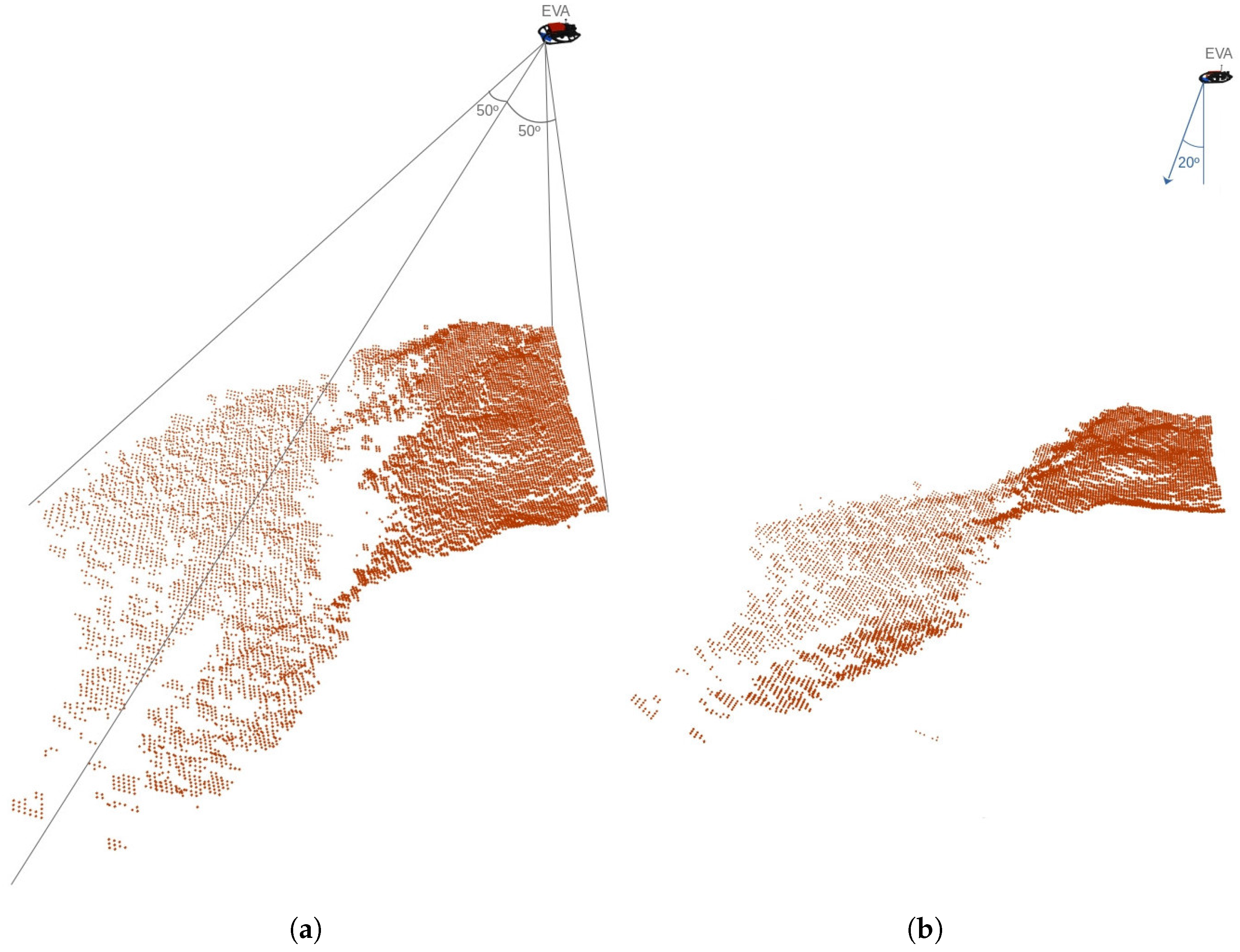
To address these issues, we investigate the possibility to integrate a 3D profiling sonar—the Echoscope 3D from Coda Octopus [15]—into a scan matching based SLAM framework. Due the heavy weight, large size and expensive price, the Echoscope 3D is not usually found onboard surveying AUVs. In fact, our EVA AUV [16], originally developed for collecting dense underwater geometric data, in the context of the ¡VAMOS! project, was specially designed to accommodate the Echoscope 3D. From a single acoustic ping, this profiling sonar insonifies a square patch of the sea floor, producing a 128 × 128 point cloud (Figure 1). With the guarantee of overlap between consecutive range scans secured, comes the opportunity to develop scan matching directly from the raw sonar measurements. This deviates from the traditional underwater SLAM trend of building submaps, whose consistency directly depends on the quality of dead reckoning. For this purpose, our 3DupIC algorithm [17] enables the registration of Echoscope 3D scans in six degrees of freedom, to obtain refined relative scan displacements as well as loop-closure constraints. All scan matching results are combined in a pose-graph to solve the SLAM problem and simultaneously calibrate the sonar extrinsic parameters. Significant improvements are obtained in terms of localization accuracy and mapping consistency.

The remainder of this paper is structured as follows. Section 2 reviews the related work on dense bathymetry SLAM, framing the contribution of this work within the context of existing research. Section 3 describes the proposed SLAM and calibration framework, detailing the factor graph formulation and the front-end algorithm that combines dead reckoning and scan matching to construct the graph. Section 4 presents the dead reckoning system, which employs an Extended Kalman Filter to fuse angular velocity measurements from gyroscopes with DVL velocity data. Section 5 explains the 3DupIC probabilistic scan matching algorithm used for 3D sonar scan registration. Section 6 describes the dataset used for experimental validation and presents a set of results characterizing the performance of the proposed method in terms of localization, mapping, and extrinsic calibration. Section 7 provides a general analysis and interpretation of the presented results. Finally, Section 8 concludes the paper and discusses directions for future research.

2. Related Work

Despite the considerable differences in the environment conditions and limitations in perception, early attempts at underwater SLAM relied on the same techniques used for terrestrial environments, such as sparse feature maps and the extended Kalman filter (EKF) data fusion framework [18]. It soon became evident the difficulty of extracting features from low-resolution sonar, so authors alleviate this challenge by populating the scene with artificial targets. The vast majority of subsequent work on feature-based sonar SLAM focus on structured man-made environments [19,20,21], where the presence of unique and distinguishable features is more likely. Feature-based approaches often use imaging sonars, whose working principle relies on vertically wide acoustic beams, which hinders the direct determination of three-dimensional information [5]. For this reason, the SLAM problem is frequently relaxed, with the estimation limited to only a few degrees of freedom [19,20,21]. When the sonar is slightly tilted down to map the seafloor at a shallow grazing angle, the flat seabed assumption is most times adopted [22,23]. For three-dimensional reconstruction, multiple frames gathered from different viewpoints can be combined using structure from motion techniques [24,25]. Alternatively, a pair of orthogonal imaging sonars allows 3D reconstruction in the overlapping area of their fields of view [26].

This work pursues a more general and environment agnostic philosophy. Instead of relying on feature extraction, we reduce measurement processing and environment modeling to a minimum and follow a dense SLAM approach. Our application is related to the so-called bathymetric SLAM problem, which involves the use of a profiling sonar to map the seabed. To accomplish this objective, the ranging sonar is pointed down, to collect successive swaths of the seafloor [27] while the vehicle performs a lawnmower trajectory pattern over the target area. Although effective for covering large areas, this configuration strongly penalizes SLAM due to the lack of measurement overlap.

To ensure continuous re-observation of the surrounding space, Fairfield et al. [28] resort to an unconventional array of pencil beam sonars, installed all around the spherical DEPTHX vehicle. In this work, a volumetric evidence grid map is used to map flooded sinkholes. The adoption of grid maps in the context of SLAM is tightly associated with Rao-Blackwellized particle filters (RBPF) [29,30]. A similar concept, but using a traditional bathymetric setup, with a multibeam echosounder (MBES), is presented by Barkby et al. [31]. With the goal of mapping the seafloor, assuming it is almost flat and devoid of vertical structures, authors employ an elevation grid map—a planar grid where each cell stores a depth estimate.

Several improvements to RBPF SLAM have been proposed for reducing computational complexity and improving performance in situations of low data overlap [14,32,33,34,35]. Additionally, maintaining a map for each particle constitutes a heavy computational overhead. In this regard, efficient data structures, to reduce the storage of redundant information and avoid expensive memory copies during resampling, are essential [28,31,36].

Another major drawback of combining grid maps with range sensors is the absence of a straightforward technique for matching new observations with the map [37]. This is essential to improve particle propagation, as suggested in FastSLAM 2.0 [38]. Earlier works studied the possibility to integrate scan matching with grid maps and RBPF SLAM [39,40]. However, scan matching operates mainly at point cloud level, so building point cloud maps facilitates the matching process. Point clouds result from the deterministic process of projecting geometric measurements in space according to their corresponding acquisition poses. Thus, the map is fully conditioned on the robot trajectory. This justifies the adoption of pose-based SLAM, a technique that removes the map from the estimation task and places full emphasis on trajectory estimation.

Earlier examples of underwater pose-based SLAM were implemented using Kalman filters [41,42,43,44]. The last decade witnessed a shift from filtering SLAM approaches, based on the Kalman filter and the RBPF, towards modern age smoothing implementations [45], formalized through factor graphs [46,47]. Smoothing methodologies address SLAM as a Maximum a Posteriori estimation problem, making use of the full measurement history to optimize the entire trajectory and enhance the map consistency. The pose-graph variant, where nodes exclusively represent robot poses, gained significant popularity in underwater applications [48,49,50,51], offering a suitable graph structure to easily integrate displacement constraints computed through scan matching.

Scan matching typically performs an iterative optimization process, seeking the transformation that best aligns overlapping sets of points. The Iterative Closest Point (ICP) [52] is one of the most popular and foundational methods for aligning point clouds. It has been previously applied for registration of Echoscope 3D scans [53]; however, nowadays, the original ICP algorithm is rarely used directly. Over the years, several variants have been introduced to increase speed, convergence and robustness to noise [54,55,56].

The pioneer work of Roman and Singh [43,44] proposed a bathymetric SLAM method relying on scan registration of MBES scan patches. The SLAM solution is developed using a delayed state EKF, whose state vector contains the current robot pose and the anchor points of each submap. Overlapping patches are subjected to pairwise registration to produce relative pose measurements.

As first demonstrated by Burguera et al. [57], following the pioneer work of Montesano et al. [58], probabilistic formulations of scan matching, that take noise into consideration during the data association and optimization stages, show superior robustness when registering noisy scans from ultrasonic sensors. These first experiments were performed in indoor environments, but soon after, probabilistic scan matching started to be applied underwater [20,59] for registration of MSIS scans, and subsequently incorporated in EKF SLAM solutions [60,61]. Previous approaches were applied in structured man-made environments, to solve SLAM in the plane. Extensions to 2.5D [41] and 3D [42,62] were proposed to solve the bathymetric SLAM problem in unstructured environments using multibeam sonars.

Following the same concept, we recently proposed the 3DupIC probabilistic scan matching algorithm [17] for the registration of scans acquired with the Echoscope 3D profiling sonar. Through a GPU parallelized implementation [63], 3DupIC achieves real-time performance, enabling onboard scan registration by the EVA AUV during its missions.

Building upon this previous work, the main contributions of the present study are as follows:

• Development of a pose-graph SLAM framework built upon the 3DupIC algorithm, which eliminates the need for submap construction, setting it apart from other scan matching based SLAM approaches. As discussed in [43], submap creation involves an inherent trade-off between size and consistency: larger submaps increase the probability of overlap but suffer from reduced internal coherence due to accumulated dead reckoning drift. By avoiding submap construction, the proposed system remains robust under degraded dead reckoning conditions and maintains high accuracy even during extended DVL outages.
• Experimental demonstration of the benefits of integrating a 3D profiling sonar within a SLAM framework, highlighting its ability to support direct scan matching odometry and reduce dependency on dead reckoning accuracy. This work provides a reference performance study, as new compact and more affordable 3D sonars, such as the Water Linked 3D-15, enter the market, making high resolution underwater SLAM increasingly feasible for a wider range of AUV platforms.
• Joint estimation of sonar extrinsic parameters within the factor graph, allowing the refinement of the sonar-to-body transformation as part of the SLAM optimization process. This unified formulation improves both localization accuracy and map consistency by ensuring that sensor alignment is refined directly within the SLAM estimation process.

3. Simultaneous Localization, Mapping and Calibration

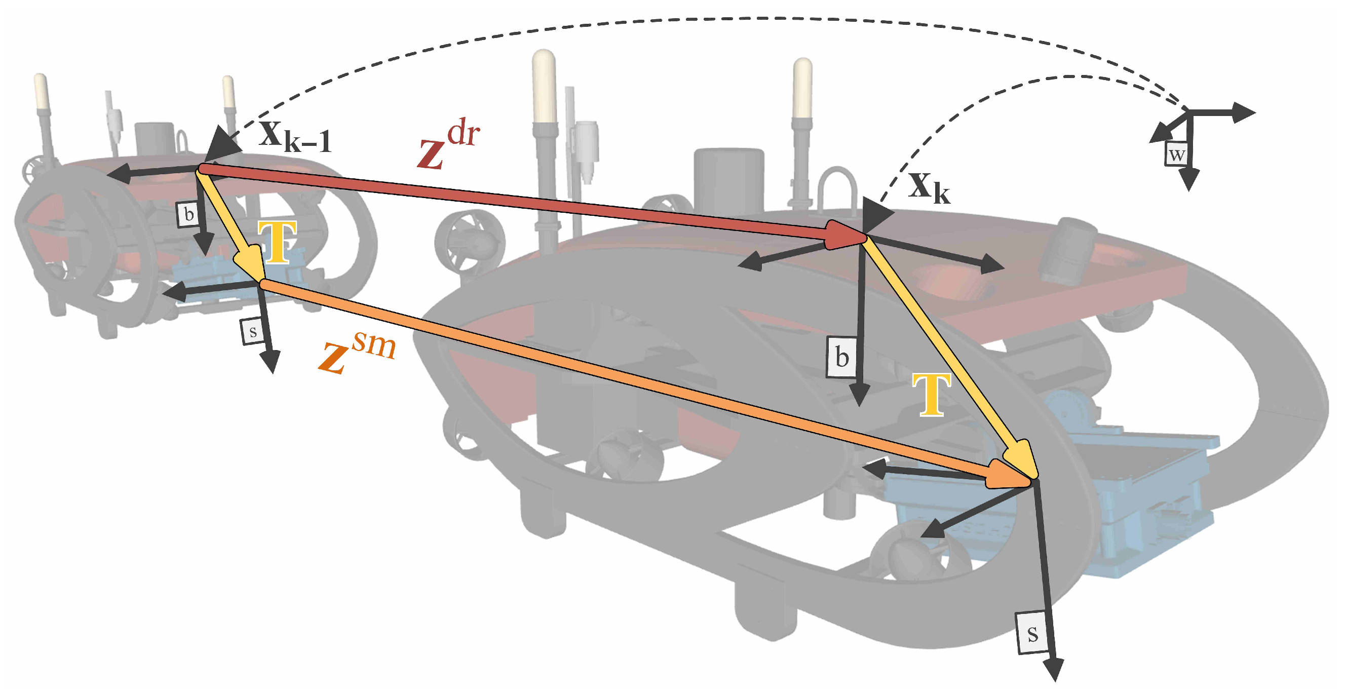
Our solution follows the pose-graph SLAM strategy, estimating the robot poses associated with scan acquisition instants. As depicted in Figure 2, the displacement between consecutive poses is measured in two different ways. On one hand, a dead reckoning estimate, ${\mathbf{z}}^{dr}$, is obtained by fusing gyroscope with DVL data using an EKF. This measurement is defined in the body reference frame (b), which is the primary reference frame used in the SLAM process to track the robot’s trajectory relative to the global world reference frame (w). On the other hand, a second displacement measurement ${\mathbf{z}}^{sm}$ is obtained through scan matching. The scan matching solution is defined in the sonar reference frame (s). The extrinsic parameters $\mathbf{T}$ establish the sonar reference frame with respect to the body reference frame. An initial estimate for $\mathbf{T}$, is available; however, evidence from previous experiments [17] reveals trajectory inconsistencies attributed to inaccurate extrinsic parameters. Accordingly, a self-calibration strategy is developed here within the SLAM framework to simultaneously optimize for $\mathbf{T}$.

A graph-based approach is employed to formulate the SLAM and calibration problems. Graph SLAM utilizes a smoothing framework where the entire measurement history is used to constrain variables during the graph optimization process. This enables the possibility to adjust linearization points and gives the opportunity to revise past data association [64]. Furthermore, it provides a suitable framework to accomplish indirect estimation of extrinsic parameters, which requires the contribution of multiple constraints to produce overdetermined problems, which can be easily expressed through factor graphs.

Graph building and graph optimization are the two major tasks within graph SLAM [46]. The block responsible for building the graph holds the robot perception capabilities, including measurement processing and data association, and is usually called front-end. The optimization block, known as back-end, acts on the graph, applying nonlinear least squares optimization techniques to refine variables according to the constraints imposed by factors. Several efficient tools are available for optimization of factor graphs including GTSAM [65], g2o [66], Ceres solver [67], between others. This work focuses on the front-end, detailing the perception techniques used to build the factor graph. For graph optimization we rely on the back-end provided by the GTSAM library.

3.1. Notation

Throughout the article, the following notation is adopted:

• $\mathbf{X}=\left\{{\mathbf{x}}_i\right\}$ represents the robot trajectory as a sequence of robot poses indexed by time $i\in \{0,\dots ,k\}$. Each pose ${\mathbf{x}}_i$ encodes the three-dimensional position and orientation of the robot’s body frame, defined with respect to the world reference frame.
• $\mathbf{Z}=\left\{{\mathbf{z}}_i^{\gamma }\right\}$ denotes the set of all measurements, where the superscript $\gamma$ is a label indicating the measuring technique, measurement type or sensor used to collect the measurement. The subscript i indicates time, with the exception of the scan matching measurements, denoted ${\mathbf{z}}_{r,t}^{\mathrm{sm}}$, where the subscripts r and t indicate the acquisition times for the reference and target scans, respectively.
• To improve readability, reference frames are usually omitted. However, when necessary for disambiguation, a preceding subscript indicates the reference frame in which a quantity is defined. For instance, _wx_i denotes a pose ${\mathbf{x}}_i$ is expressed in the world reference frame w.
• A preceding superscript can be used to indicate the destination frame. For example, extrinsic parameters can be expressed as ${}_b{}^s\mathbf{T}$, explicitly denoting a transformation from the body frame b to the sonar frame s.
• Poses, extrinsic parameters and displacements $\mathbf{q}$ are defined with six degrees of freedom, comprising three-dimensional translation and orientation components. The operator $\mathbf{R}\left\{\mathbf{q}\right\}$ returns the orientation part, in rotation matrix form, while $\mathbf{t}\left\{\mathbf{q}\right\}$ extracts a translation vector.
• ⊕ and ⊖ indicate the additive and subtractive frame composition operations, as defined in [68].

3.2. Factor Graph Formulation

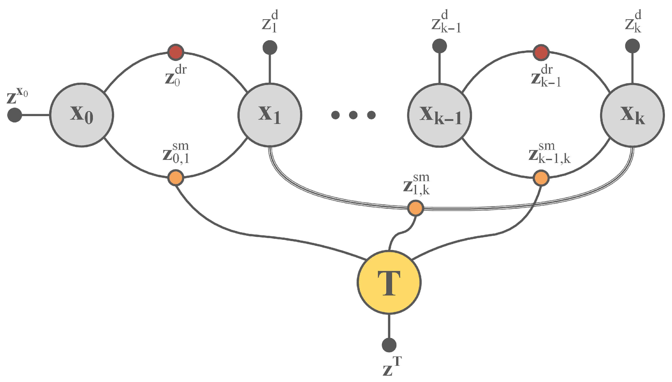
The simultaneous estimation of the robot trajectory $\mathbf{X}$ and the transformation $\mathbf{T}$ is accomplished using the factor graph illustrated in Figure 3. The robot trajectory is represented in the factor graph as a sequence of nodes, each corresponding to a vehicle pose at which a sonar scan was acquired. Edges in the factor graph define probabilistic constraints derived from sensor measurements $\mathbf{Z}$. In our particular implementation, and according to Figure 3, the following factors are established:

• An initialization measurement ${\mathbf{z}}^{{\mathbf{x}}_0}$ anchors the first pose with respect to the world reference frame, following expression: ${\mathbf{z}}^{{\mathbf{x}}_0}={\mathbf{x}}_0+{\omega }^{{\mathbf{x}}_0}$, where ${\omega }^{{\mathbf{x}}_0}$ is an additive zero mean noise vector with covariance ${\mathbf{\Sigma }}^{{\mathbf{x}}_0}$. Under Gaussian assumption, this prior factor follows a normal distribution: $P\left({\mathbf{x}}_0\right)\propto \mathcal{N}\left({\mathbf{z}}^{{\mathbf{x}}_0},{\mathbf{\Sigma }}^{{\mathbf{x}}_0}\right)$. To promote a fair evaluation of our method, the initial pose measurement is retrieved from the ground-truth trajectory. In a field application, full pose initialization, including position and attitude, can be obtained from the combination of accelerometers and a multiple antenna GNSS system [6]. It is worth noting that inaccuracies in the initial pose primarily affect the global georeferencing of the resulting trajectory and map, but do not compromise the relative accuracy or convergence properties of the proposed SLAM formulation, which is driven by relative constraints derived from scan matching and dead reckoning.
• The unary factor ${\mathbf{z}}^{\mathbf{T}}$ specifies the initial extrinsic parameter values. Under Gaussian assumption, this factor establishes the prior probability: $P\left(\mathbf{T}\right)\propto \mathcal{N}\left({\mathbf{z}}^{\mathbf{T}},{\mathbf{\Sigma }}^{\mathbf{T}}\right)$, being ${\mathbf{\Sigma }}^{\mathbf{T}}$ the covariance matrix describing the initial uncertainty.
• The vertical position of each pose node is constrained by a depth measurement $z_k^d$, obtained from a pressure sensor. The unary factor follows the relation $z_k^d=f\left({\mathbf{x}}_k\right)+{\omega }_k^d$, where function $f\left({\mathbf{x}}_k\right)$ extracts the robot depth from pose ${\mathbf{x}}_k$ and ${\omega }_k^d$ is the white Gaussian noise with variance ${\sigma }^2$. The resulting conditional probability is expressed as: $P\left(z_k^d|{\mathbf{x}}_k\right)\propto \exp \left(-{\displaystyle \frac{1}{2}}{∥{f\left({\mathbf{x}}_k\right)-z}_k^d∥}_{{\sigma }^2}^2\right)$
• The dead reckoning factor relates two consecutive poses ${\mathbf{x}}_{k-1}$ and ${\mathbf{x}}_k$ with a displacement measurement ${\mathbf{z}}_k^{dr}$ through the following expression: ${\mathbf{x}}_k={\mathbf{x}}_{k-1}\oplus {\mathbf{z}}_k^{dr}+{\omega }_k^{dr}$, being ${\omega }_k^{dr}$ an additive noise vector. Assuming the displacement measurement is affected by white Gaussian noise with covariance ${\mathbf{\Sigma }}_k^{dr}$, the probability of a new pose ${\mathbf{x}}_k$ given ${\mathbf{x}}_{k-1}$ and ${\mathbf{z}}_k^{dr}$ follows a Gaussian distribution: $P\left({\mathbf{x}}_k|{\mathbf{x}}_{k-1},{\mathbf{z}}_k^{dr}\right)\propto \exp \left(-{\displaystyle \frac{1}{2}}{∥{\mathbf{x}}_{k-1}\oplus {\mathbf{z}}_k^{dr}-{\mathbf{x}}_k∥}_{{\mathbf{\Sigma }}_k^{dr}}^2\right)$.
• In the scan matching process, the target scan acquired from robot pose ${\mathbf{x}}_t$ is registered with respect to the reference scan, obtained from pose ${\mathbf{x}}_r$, to compute a displacement measurement ${\mathbf{z}}_{r,t}^{sm}$. As illustrated in Figure 2, the scan matching result is defined in the sonar reference frame, therefore, in order to constrain ${\mathbf{x}}_r$ and ${\mathbf{x}}_t$ through ${\mathbf{z}}_{r,t}^{sm}$ the extrinsic parameters are applied: ${\mathbf{z}}_{r,t}^{sm}=\left(\left({\mathbf{x}}_t\ominus {\mathbf{x}}_r\right)\oplus \mathbf{T}\right)\ominus \mathbf{T}+{\omega }_{r,t}^{sm}$, where ${\omega }_{r,t}^{sm}$ is a noise vector characterizing the measurement’s uncertainty. Assuming a Gaussian measurement model, the conditional probability follows a normal distribution: $P\left({\mathbf{z}}_{r,t}^{sm}|{\mathbf{x}}_r,{\mathbf{x}}_t,\mathbf{T}\right)\propto \exp \left(-{\displaystyle \frac{1}{2}}{∥\left(\left({\mathbf{x}}_t\ominus {\mathbf{x}}_r\right)\oplus \mathbf{T}\right)\ominus \mathbf{T}-{\mathbf{z}}_{r,t}^{sm}∥}_{{\mathbf{\Sigma }}_{r,t}^{sm}}^2\right)$

The factor graph from Figure 3 represents the joint distribution over poses $\mathbf{X}$, measurements $\mathbf{Z}$ and extrinsic parameters $\mathbf{T}$:

$$P\left(\mathbf{X},\mathbf{T},\mathbf{Z}\right)=P\left({\mathbf{x}}_0\right)P\left(\mathbf{T}\right)\prod _{k}P\left(z_k^d|{\mathbf{x}}_k\right)\prod _{k}P\left({\mathbf{x}}_k|{\mathbf{x}}_{k-1},{\mathbf{z}}_k^{dr}\right)\prod _{r,t}P\left({\mathbf{z}}_{r,t}^{sm}|{\mathbf{x}}_r,{\mathbf{x}}_t,\mathbf{T}\right)$$

(1)

The optimization step, part of the back-end, seeks the configuration of robot poses ${\mathbf{X}}^{*}$ and extrinsic parameters ${\mathbf{T}}^{*}$ that maximizes the joint distribution:

$$\left\{{\mathbf{X}}^{*},{\mathbf{T}}^{*}\right\}=\arg \underset{\{\mathbf{X},\mathbf{T}\}}{\max }P\left(\mathbf{X},\mathbf{T},\mathbf{Z}\right)$$

(2)

Under Gaussian assumption, the maximum a posteriori (MAP) estimate $\left\{{\mathbf{X}}^{*},{\mathbf{T}}^{*}\right\}$ can be solved through a non-linear least squares problem [69]. In this work, the Square Root SAM algorithm [69], provided by the GTSAM library [65], is used to optimize the factor graph.

3.3. Front-End Algorithm

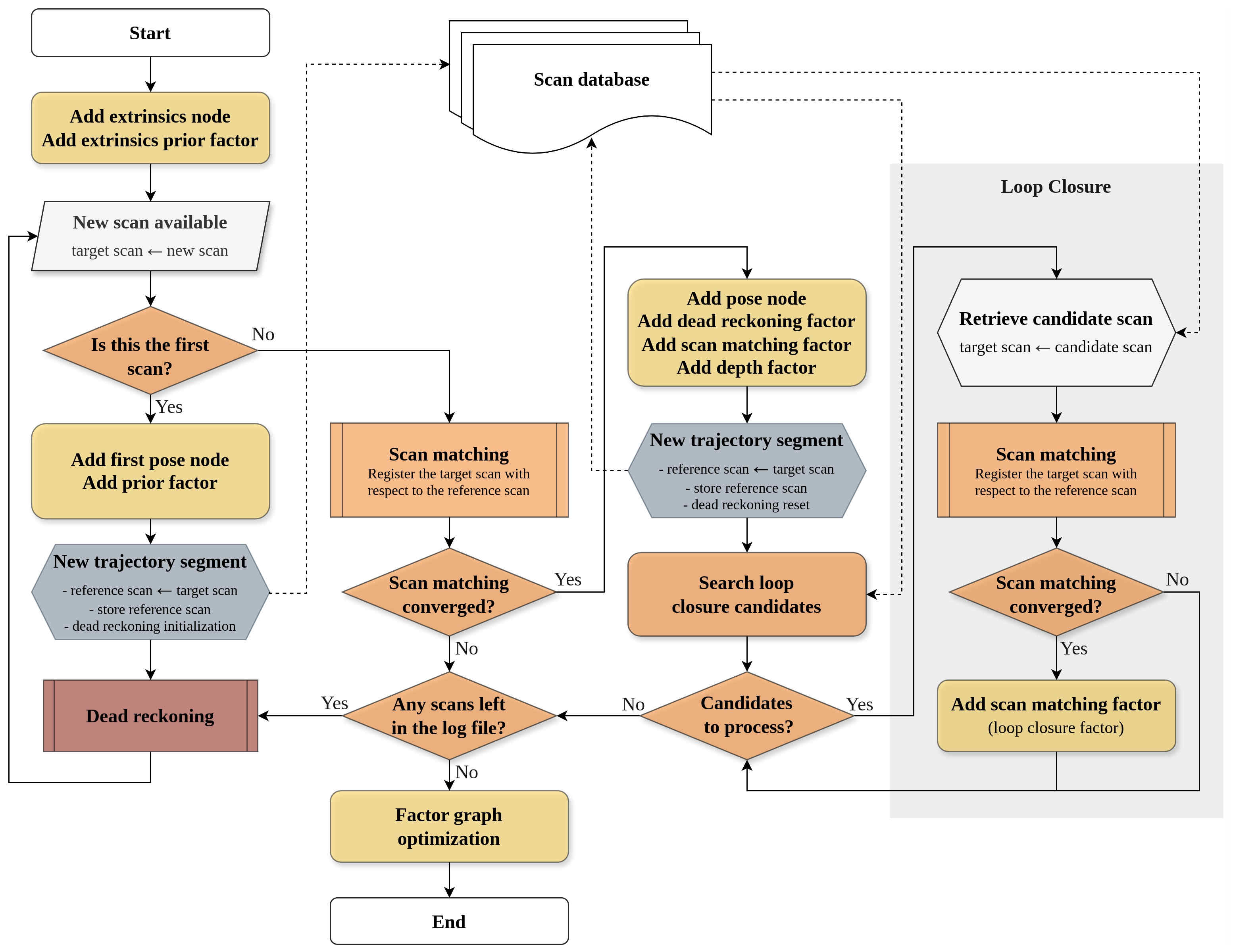
Initialization and depth measurements can be readily obtained from ground-truth, prior calibration or direct sensor readings. In contrast, displacement observations derived from dead reckoning and scan matching require more elaborate processing routines. Although these two methods generate independent factors within the graph, they are not entirely decoupled from a computational perspective. Instead, they operate synergistically, interacting and sharing intermediate results. All those relations are expressed in the flowchart from Figure 4, that provides a high-level overview of the front-end algorithm.

The process starts with the insertion of the extrinsic parameters node in the factor graph. A prior factor is also included to specify an initial estimate for this transformation.

Next, the first scan is loaded and assigned the label of target scan. Scans inside the registration process assume different roles: the reference scan remains static, while the registration method computes and applies a transformation to the target scan, maximizing its overlap with respect to the reference. Only scans with acquisition poses presented in the factor graph can serve as references, while new scans entering the SLAM process take the target role first. After loading the first scan, the initial pose node is added to the factor graph along with the corresponding prior factor. The insertion of a pose node concludes the estimation of one trajectory segment and marks the begging of a new one, where the robot trajectory is computed until a new scan arrives and becomes successfully registered. This involves a context switch operation, where the target scan is reassigned as reference and integrated into the sonar scan database. The dead reckoning estimate is reset, so that, in the next phase, the robot is localized with respect to the latest pose in the factor graph, until a new scan is acquired.

With the arrival of a new scan, and taking the dead reckoning estimate as initialization, the registration process is executed and the convergence is evaluated. If divergence occurs, the target scan is discarded and the trajectory segment continues, using dead reckoning to track the robot pose until a new scan enters the system. Contrarily, in case of convergence, a new pose node is inserted and a depth measurement is taken to produce a depth factor. Both poses become connected by a dead reckoning factor specifying the estimated displacement. Additionally, the scan matching solution is inserted through a ternary factor, relating both scan acquisition poses and the extrinsic parameter transformation.

The addition of a pose node marks the transition to a new trajectory segment. This implies the replacement of the reference scan and the reset of the dead reckoning estimate. During reset, the dead reckoning pose is set to the origin, except for velocity states, which are initialized with a velocity measurement obtained by differentiation of the displacement previously computed by scan matching.

The final stage executes the loop-closure routine, searching the scan database for candidate scans, based on their spatial proximity to the current reference scan. Each candidate is sequentially retrieved and registered against the reference scan. If convergence is achieved, a new loop-closure constraint is added to the factor graph. The algorithm then resumes, performing dead reckoning estimation until a new scan becomes available.

Once all scans in the log file have been processed, the back-end is called to optimize the factor graph, marking the completion of the simultaneous localization, mapping, and calibration process. Expected outcomes of this process include an improved trajectory estimation and a refined calibration of the extrinsic parameters. Subsequently, taking advantage of more accurate trajectory and extrinsics, the point cloud map can be reconstructed to improve its consistency.

4. Dead Reckoning

The dead reckoning measurement in the SLAM and calibration factor graph relates two consecutive scan acquisition poses. Therefore, the last pose in the factor graph establishes the reference frame for the new trajectory segment, relative to which robot position and orientation is defined. To compute the robot displacement, an extended Kalman filter (EKF) is used, fusing periodic angular velocity measurements from gyroscopes with asynchronous linear velocity observations from DVL.

At time step t, the displacement is expressed by a nine element state vector ${\mathbf{z}}_t^{dr}={[{\mathbf{p}}_t^{dr},{\mathit{\alpha }}_t^{dr},{\mathit{\nu }}_t^{dr}]}^{\top }$, where ${\mathbf{p}}_t^{dr}={[x_t^{dr},y_t^{dr},z_t^{dr}]}^{\top }$, ${\mathit{\alpha }}_t^{dr}={[{\varphi }_t^{dr},{\theta }_t^{dr},{\psi }_t^{dr}]}^{\top }$ and ${\mathit{\nu }}_t^{dr}={[u_t^{dr},v_t^{dr},w_t^{dr}]}^{\top }$ denote the three-dimensional position, Euler angle orientation and three-dimensional velocity, respectively. Unlike position and orientation, velocity states are defined in the robot’s body frame.

4.1. Initialization and State Reset

The beginning of a new trajectory segment involves a state and covariance reset, affecting position and orientation states. For the initial segment, velocity is initialized using the first DVL observation; in alternative, for subsequent segments, it can also be computed from the displacement obtained through scan matching. This last approach, illustrated in Figure 5, is particularly useful in situations where the DVL performance is compromised, offering a way to keep a consistent velocity estimate.

To compute the body-frame velocity ${\mathit{\nu }}_k$, at the end of trajectory segment k, the displacement computed from scan matching ${}_s\mathbf{z}_{k-1,k}^{\mathit{sm}}$ is first transformed from the sonar reference frame to the body reference frame, by compounding the displacement pose with the extrinsic parameters:

$${}_b\mathbf{z}_{k-1,k}^{\mathit{sm}}=\left(\mathit{T}\oplus {}_s\mathbf{z}_{k-1,k}^{\mathit{sm}}\right)\ominus \mathit{T}$$

(3)

To obtain the robot velocity in the body frame, a rotation is applied to the position displacement, followed by numerical differentiation:

$${\mathit{\nu }}_k={\displaystyle \frac{\mathbf{R}{\{}_b{\mathbf{z}}_{k-1,k}^{sm}\}·\mathbf{t}{\{}_b{\mathbf{z}}_{k-1,k}^{sm}\}}{\Delta t_{k-1,k}}}$$

(4)

where $\Delta t_{k-1,k}$ is the time interval between poses ${\mathbf{x}}_{k-1}$ and ${\mathbf{x}}_k$.

4.2. Prediction

A constant velocity model is used for propagation of velocity and position states. Orientation is predicted through integration of gyroscope angular velocity measurements $\omega$ using a simple inertial mechanization technique. The complete motion model is:

$${\mathbf{z}}_t^{dr}=\left[\begin{array}{c}{\mathbf{p}}_t^{dr}\\ {\mathit{\alpha }}_t^{dr}\\ {\mathit{\nu }}_t^{dr}\end{array}\right]=\left[\begin{array}{c}{\mathbf{p}}_{t-1}^{dr}+\mathbf{R}\left\{{\mathit{\alpha }}_{t-1}^{dr}\right\}·{\mathit{\nu }}_{t-1}^{dr}.\Delta t\\ {\mathit{\alpha }}_{t-1}^{dr}+\mathbf{E}\left\{{\mathit{\alpha }}_{t-1}^{dr}\right\}·{\omega }_t.\Delta t\\ {\mathit{\nu }}_{t-1}^{dr}\end{array}\right]$$

(5)

being $\Delta t$ the period of the prediction step, dictated by the gyroscope data rate. Matrix $\mathbf{E}\left\{{\mathit{\alpha }}_{t-1}^{dr}\right\}$ converts angular velocities into Euler angles rate of change:

$$\mathbf{E}\left\{{\mathit{\alpha }}_{t-1}^{dr}\right\}=\left[\begin{array}{ccc}1& \sin \left({\varphi }_{t-1}^{dr}\right)\tan \left({\theta }_{t-1}^{dr}\right)& \cos \left({\varphi }_{t-1}^{dr}\right)\tan \left({\theta }_{t-1}^{dr}\right)\\ 0& \cos \left({\varphi }_{t-1}^{dr}\right)& -\sin \left({\varphi }_{t-1}^{dr}\right)\\ 0& \sin \left({\varphi }_{t-1}^{dr}\right)\sec \left({\theta }_{t-1}^{dr}\right)& \cos \left({\varphi }_{t-1}^{dr}\right)\sec \left({\theta }_{t-1}^{dr}\right)\end{array}\right]$$

(6)

The error covariance matrix ${\mathbf{\Sigma }}^{dr}$ is projected using the standard EKF expression:

$${\mathbf{\Sigma }}_t^{dr}={\mathbf{F}}_t{\mathbf{\Sigma }}_{t-1}^{dr}{\mathbf{F}}_t^{\top }+{\mathbf{G}}_t{\mathbf{Q}}_t{\mathbf{G}}_t^{\top }$$

(7)

where ${\mathbf{Q}}_t$ a 6 by 6 diagonal matrix specifying the noises associated with the linear and angular velocities. Matrix ${\mathbf{F}}_t$ is the Jacobian matrix of the motion model with respect to the state vector (Equation (8)). Matrix ${\mathbf{G}}_t$ is the Jacobian of the motion model with respect to linear and angular velocities (Equation (9)). To produce a reliable estimation of pose uncertainty, particularly to ensure it increases monotonically, correlations must be avoided between velocity states and the others. Otherwise, velocity measurements incorporated during the update step may alter pose states and reduce their uncertainty, leading to an overconfident estimate. Correlation is prevented by setting to zero the 3 by 3 upper right and bottom left corners from matrices ${\mathbf{F}}_t$ and ${\mathbf{G}}_k$ as follows:

$${\mathbf{F}}_t={\left[\begin{array}{ccc}{\displaystyle \frac{\partial {\mathbf{p}}_t^{dr}}{\partial {\mathbf{p}}_t^{dr}}}& {\displaystyle \frac{\partial {\mathbf{p}}_t^{dr}}{\partial {\mathit{\alpha }}_t^{dr}}}& {\overline{){\displaystyle \frac{\partial {\mathbf{p}}_t^{dr}}{\partial {\mathit{\nu }}_t^{dr}}}}}^0\\ ine{\displaystyle \frac{\partial {\mathit{\alpha }}_t^{dr}}{\partial {\mathbf{p}}_t^{dr}}}& {\displaystyle \frac{\partial {\mathit{\alpha }}_t^{dr}}{\partial {\mathit{\alpha }}_t^{dr}}}& {\displaystyle \frac{\partial {\mathit{\alpha }}_t^{dr}}{\partial {\mathit{\nu }}_t^{dr}}}\\ ine{\overline{){\displaystyle \frac{\partial {\mathit{\nu }}_t^{dr}}{\partial {\mathbf{p}}_t^{dr}}}}}^0& {\displaystyle \frac{\partial {\mathit{\nu }}_t^{dr}}{\partial {\mathit{\alpha }}_t^{dr}}}& {\displaystyle \frac{\partial {\mathit{\nu }}_t^{dr}}{\partial {\mathit{\nu }}_t^{dr}}}\end{array}\right]}_{\left[9\times 9\right]}=\left[\begin{array}{ccc}{\mathbf{I}}_{\left[3\times 3\right]}& {{\displaystyle \frac{\partial {\mathbf{p}}_t^{dr}}{\partial {\mathit{\alpha }}_t^{dr}}}}_{\left[3\times 3\right]}& {\mathbf{0}}_{\left[3\times 3\right]}\\ ine{\mathbf{0}}_{\left[3\times 3\right]}& {{\displaystyle \frac{\partial {\mathit{\alpha }}_t^{dr}}{\partial {\mathit{\alpha }}_t^{dr}}}}_{\left[3\times 3\right]}& {\mathbf{0}}_{\left[3\times 3\right]}\\ ine{\mathbf{0}}_{\left[3\times 3\right]}& {\mathbf{0}}_{\left[3\times 3\right]}& {\mathbf{I}}_{\left[3\times 3\right]}\end{array}\right]$$

(8)

$${\mathbf{G}}_t={\left[\begin{array}{cc}{\displaystyle \frac{\partial {\mathbf{p}}_t^{dr}}{\partial {\mathit{\nu }}_t^{dr}}}& {\overline{){\displaystyle \frac{\partial {\mathbf{p}}_t^{dr}}{\partial {\omega }_t^{dr}}}}}^0\\ ine{\displaystyle \frac{\partial {\mathit{\alpha }}_t^{dr}}{\partial {\mathit{\nu }}_t^{dr}}}& {\displaystyle \frac{\partial {\mathit{\alpha }}_t^{dr}}{\partial {\omega }_t^{dr}}}\\ ine{\overline{){\displaystyle \frac{\partial {\mathit{\nu }}_t^{dr}}{\partial {\mathit{\nu }}_t^{dr}}}}}^0& {\displaystyle \frac{\partial {\mathit{\nu }}_t^{dr}}{\partial {\omega }_t^{dr}}}\end{array}\right]}_{\left[9\times 6\right]}=\left[\begin{array}{cc}{\mathbf{R}\left\{{\mathit{\alpha }}_{t-1}^{dr}\right\}·\Delta t}_{\left[3\times 3\right]}& {\mathbf{0}}_{\left[3\times 3\right]}\\ ine{\mathbf{0}}_{\left[3\times 3\right]}& {\mathbf{E}\left\{{\mathit{\alpha }}_{t-1}^{dr}\right\}·\Delta t}_{\left[3\times 3\right]}\\ ine{\mathbf{0}}_{\left[3\times 3\right]}& {\mathbf{0}}_{\left[3\times 3\right]}\end{array}\right]$$

(9)

4.3. Update

In the update step, velocity states are corrected based on asynchronous DVL observations in the body frame: ${\mathbf{z}}_t^{DVL}=\left[u_t^{DVL},v_t^{DVL},w_t^{DVL}\right]$. A direct state observation is performed using the standard EKF equations with the following observation matrix.

$$\mathbf{H}=\left[\begin{array}{cc}{\mathbf{0}}_{\left[3\times 6\right]}& {\mathbf{I}}_{\left[3\times 3\right]}\end{array}\right]$$

(10)

Since the prediction stage prevents correlations between velocity and other states, corrections applied at this stage affect only the velocity states, keeping position and attitude estimates unchanged.

5. Scan Matching

Scan matching is applied to estimate the robot’s displacement between scan acquisition poses. To this end, pairs of sonar scans acquired with an Echoscope 3D sonar are registered using the 3DupIC scan matching algorithm [17]. The method consists of four main stages: first, a probabilistic model is constructed for each scan; second, an initial displacement estimate is obtained from the dead reckoning solution; third, a matching step identifies compatible point correspondences between the scans; and finally, a refined displacement estimate is computed by minimizing the Mahalanobis distances between matched points. The last two steps are repeated iteratively until convergence or until a maximum number of iterations is reached.

5.1. Probabilistic Scan Modeling

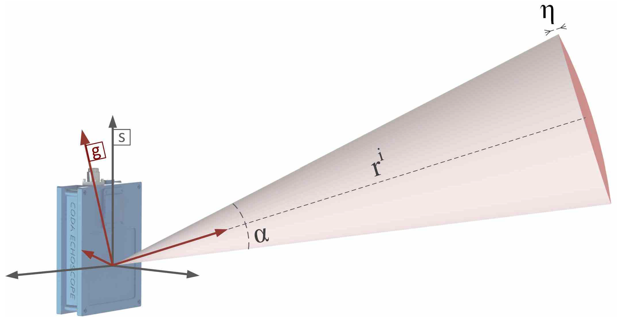
From a single ping, the Echoscope 3D sonar retrieves a $128\times 128$ matrix of range measurements, from which a 3D point cloud scan is generated (Figure 1). The uncertainty model is an adaptation of the formulation proposed in [57], originally defined for a two-dimensional sonar beam. We extend this model to three dimensions to accurately represent the conical beam geometry characteristic of profiling sonars, as illustrated in Figure 6. Considering the beam’s angular aperture $\mathit{\alpha }$, the area of beam incidence increases with the measured range r, causing ambiguity in the plane normal to the beam direction. Along the beam axis, uncertainty is primarily determined by the sensor’s range resolution $\eta$. The spatial uncertainty of each measurement is modeled probabilistically, with the lateral standard deviation encompassing approximately 99.7% of the expected beam footprint, and the axial standard deviation defined by the range resolution.

Accordingly, the ith beam of a given scan is modeled as a Gaussian random variable ${}_{g}b^i=\mathcal{N}({}_g\mathbf{b}^i,{}_g\mathbf{\Sigma }^i)$, where the mean ${}_g\mathbf{b}^i$ is directly defined by the measured range $r^i$, along the Z-axis: ${}_g\mathbf{b}^i={[0,0,r^i]}^{\top }$. In its local beam reference frame g, with the Z-axis passing through the center of the cone (Figure 6), the ith beam uncertainty is characterized by the following covariance matrix:

$${}_g\mathbf{\Sigma }^i=\left[\begin{array}{ccc}{\left(r^i·\tan \left(\alpha /2\right)\right)}^2& 0& 0\\ 0& {\left(r^i·\tan \left(\alpha /2\right)\right)}^2& 0\\ 0& 0& {\left(\eta /2\right)}^2\end{array}\right]$$

(11)

The probabilistic model for the entire scan $\mathcal{S}$ is defined as the collection of all beam distributions expressed in the sonar reference frame:

$$\mathcal{B}={\left\{{}_{s}b^i\sim \mathcal{N}\left({}_s\mathbf{b}^i,{}_s\mathbf{\Sigma }^i\right)\right\}}_{i=1}^{128\times 128}$$

(12)

Each measurement is transformed into the sonar frame by applying a beam-specific rotation matrix ${}_g{}^s\mathbf{R}^i$, which is defined according to the direction of the corresponding beam [17]:

$${}_s\mathbf{b}^i=\left({}_g{}^s\mathbf{R}^i\right)·\left({}_g\mathbf{b}^i\right),{}_s\mathbf{\Sigma }^i=\left({}_g{}^s\mathbf{R}^i\right)·\left({}_g\mathbf{\Sigma }^i\right)·\left({{}_g{}^s\mathbf{R}^i}^{\top }\right)$$

(13)

5.2. Displacement Initialization

To facilitate convergence, an initial estimate of the robot displacement is provided to the scan matching algorithm. This estimate is obtained by transforming the dead reckoning displacement from the body frame to the sonar reference frame using the extrinsic parameters:

$${}_s\mathbf{z}^{\mathit{dr}}=\left({}_b\mathbf{z}^{\mathit{dr}}\oplus \mathbf{T}\right)\ominus \mathbf{T}$$

(14)

Furthermore, the 3DupIC method incorporates the uncertainty of the displacement during the matching and optimization phases. Accordingly, the covariance matrix associated with the dead reckoning displacement is transformed into the sonar reference frame via the adjoint transformation of the inverse extrinsic parameters:

$${}_s\mathbf{\Sigma }^{\mathit{dr}}=\left({\mathbf{Ad}}_{T^{-1}}\right)·\left({}_b\mathbf{\Sigma }^{\mathit{dr}}\right)·\left({\mathbf{Ad}}_{T^{-1}}^{\top }\right)$$

(15)

where ${\mathbf{Ad}}_{T^{-1}}$ denotes the adjoint matrix evaluated at the inverse of the extrinsic transformation, as detailed in [70].

5.3. Point Matching

Consider the reference scan

$$\mathcal{R}={\left\{r^j\sim \mathcal{N}\left({\mathbf{r}}^j,{\mathbf{\Sigma }}^j\right)\right\}}_{j=1}^N$$

(16)

modeled according to the probabilistic sensor model and acquired at time r from robot pose ${\mathbf{x}}_r$, where N is the number of individual beams forming one scan ($128\times 128$ for the Echoscope 3D). At time t, a target scan

$$\mathcal{T}={\left\{t^i\sim \mathcal{N}\left({\mathbf{t}}^i,{\mathbf{\Sigma }}^i\right)\right\}}_{i=1}^N$$

(17)

is collected at pose ${\mathbf{x}}_t$.

The statistical compatibility between each measurement ${\mathbf{t}}^i$ and elements in $\mathcal{R}$ is analyzed using the squared Mahalanobis distance:

$${\left(d^{ij}\right)}^2={\left({\mathit{\varrho }}^{ij}\right)}^{\top }{\left({\mathbf{\Sigma }}^{ij}\right)}^{-1}{\mathit{\varrho }}^{ij}$$

(18)

where:

$${\mathit{\varrho }}^{ij}=f\left({\mathbf{z}}_{r,t}^{sm},{\mathbf{t}}^i\right)-{\mathbf{r}}^j$$

(19)

represents the error between the jth reference point and the ith target point, evaluated in the reference scan frame. The function $f\left({\mathbf{z}}_{r,t}^{sm},{\mathbf{t}}^i\right)=\mathbf{R}\left\{{\mathbf{z}}_{r,t}^{sm}\right\}·{\mathbf{t}}^i+\mathbf{t}\left\{{\mathbf{z}}_{r,t}^{sm}\right\}$ transforms the target point, from the sonar reference frame at time t to that at time r, using the current displacement estimate ${\mathbf{z}}_{r,t}^{sm}$. In the first iteration, ${\mathbf{z}}_{r,t}^{sm}$ is initialized from the dead reckoning solution (Equation (14)), and in subsequent iterations it is updated with the last estimate computed by scan matching.

The uncertainty characterizing the matching between point i and j is represented by the covariance matrix ${\mathbf{\Sigma }}^{ij}$, which depends on the uncertainty of the individual beams (${}_s\mathbf{\Sigma }_t^i$ and ${}_s\mathbf{\Sigma }_r^j$) and on the uncertainty of the displacement ${\mathbf{\Sigma }}_{r,t}^{sm}$, according to Equation (20).

$${\mathbf{\Sigma }}^{ij}={}_s\mathbf{\Sigma }_r^j+{\mathbf{J}}_{{\mathbf{z}}_{r,t}^{sm}}\left({\mathbf{\Sigma }}_{r,t}^{sm}\right){\mathbf{J}}_{{\mathbf{z}}_{r,t}^{sm}}^{\top }.+{\mathbf{J}}_{{\mathbf{t}}^i}\left({}_s\mathbf{\Sigma }_t^i\right){\mathbf{J}}_{{\mathbf{t}}^i}^{\top }$$

(20)

Jacobian matrices ${\mathbf{J}}_{{\mathbf{z}}_{r,t}^{sm}}$ and ${\mathbf{J}}_{{\mathbf{t}}^i}$ are obtained by taking the partial derivatives of Equation (19) with respect to ${\mathbf{z}}_{r,t}^{sm}$ and ${\mathbf{t}}^i$, respectively, and evaluated at ${\mathbf{z}}_{r,t}^{sm}$ and ${\mathbf{t}}^i$:

$${\mathbf{J}}_{{\mathbf{z}}_{r,t}^{sm}}={\left.{\displaystyle \frac{\delta {\mathit{\varrho }}^{ij}}{\delta {\mathbf{z}}_{r,t}^{sm}}}\right|}_{\begin{array}{c}{\mathbf{t}}^i\\ {\mathbf{z}}_{r,t}^{sm}\end{array}}$$

(21)

$${\mathbf{J}}_{{\mathbf{t}}^i}={\left.{\displaystyle \frac{\delta {\mathit{\varrho }}^{ij}}{\delta {\mathbf{t}}^i}}\right|}_{\begin{array}{c}{\mathbf{t}}^i\\ {\mathbf{z}}_{r,t}^{sm}\end{array}}$$

(22)

The squared Mahalanobis distance follows a chi-squared distribution ${\chi }_q^2$, where q is the dimensionality of the residual vector ${\varrho }_{ij}$—in this case, $q=3$. A reference point ${\mathbf{r}}^j$ is statistically compatible with a target point ${\mathbf{t}}^i$ if the chi-squared test is satisfied, i.e., if the squared Mahalanobis distance is less than the inverse chi-squared cumulative function evaluated at confidence level $\alpha$, that is

$${\left(d^{ij}\right)}^2<{\chi }_{q,\alpha }^2$$

(23)

Among all compatible reference points, only the one with the smallest Mahalanobis distance is selected to form a match with ${\mathbf{t}}^i$. Each point correspondence is then defined as

$$\langle {\mathbf{r}}^j,{\mathbf{t}}^i\rangle |{\mathbf{r}}^j=\underset{j}{\arg \min }{\left(d^{ij}\right)}^2,{\left(d^{ij}\right)}^2<{\chi }_{q,\alpha }^2$$

(24)

By repeating this search for all points in the target scan, and assuming sufficient scan overlap, a set of correspondences is obtained:

$$\mathbf{M}=\{<{\mathbf{r}}^{\kappa 1},{\mathbf{t}}^{\kappa 1}>,\dots ,<{\mathbf{r}}^{\kappa n},{\mathbf{t}}^{\kappa n}>\}$$

(25)

where, for simplicity, $\kappa i$ represents the index pairing for the ith correspondence.

Optimization

The optimization step aims to refine the robot displacement by minimizing the squared Mahalanobis distances between corresponding points:

$${\mathbf{z}}_{r,t}^{sm}=\min \sum _{i=1}^n{\left({\mathit{\varrho }}^{\kappa i}\right)}^{\top }{\left({\mathbf{\Sigma }}^{\kappa i}\right)}^{-1}{\mathit{\varrho }}^{\kappa i}.$$

(26)

Equation (26) has a closed from solution given by

$${\mathbf{z}}_{r,t}^{sm}={\left({\mathbf{J}}^{\top }\mathbf{Q}\mathbf{J}\right)}^{-1}{\mathbf{J}}^{\top }\mathbf{Q}\mathbf{A}$$

(27)

where

$$\mathbf{J}=\left[\begin{array}{c}{\left.{\displaystyle \frac{\delta {\mathit{\varrho }}^{\kappa 1}}{\delta {\mathbf{z}}_{r,t}^{sm}}}\right|}_{\begin{array}{c}{\mathbf{t}}^{\kappa 1}\\ {\mathbf{z}}_{r,t}^{sm}\end{array}}\\ {\left.{\displaystyle \frac{\delta {\mathit{\varrho }}^{\kappa 2}}{\delta {\mathbf{z}}_{r,t}^{sm}}}\right|}_{\begin{array}{c}{\mathbf{t}}^{\kappa 2}\\ {\mathbf{z}}_{r,t}^{sm}\end{array}}\\ ⋮\\ {\left.{\displaystyle \frac{\delta {\mathit{\varrho }}^{\kappa n}}{\delta {\mathbf{z}}_{r,t}^{sm}}}\right|}_{\begin{array}{c}{\mathbf{t}}^{\kappa n}\\ {\mathbf{z}}_{r,t}^{sm}\end{array}}\end{array}\right],\mathbf{A}=\left[\begin{array}{c}\left({\left.{\displaystyle \frac{\delta {\mathit{\varrho }}^{\kappa 1}}{\delta {\mathbf{z}}_{r,t}^{sm}}}\right|}_{\begin{array}{c}{\mathbf{t}}^{\kappa 1}\\ {\mathbf{z}}_{r,t}^{sm}\end{array}}\right)·{\mathbf{z}}_{r,t}^{sm}-{\mathit{\varrho }}^{\kappa 1}\\ \left({\left.{\displaystyle \frac{\delta {\mathit{\varrho }}^{\kappa 2}}{\delta {\mathbf{z}}_{r,t}^{sm}}}\right|}_{\begin{array}{c}{\mathbf{t}}^{\kappa 2}\\ {\mathbf{z}}_{r,t}^{sm}\end{array}}\right)·{\mathbf{z}}_{r,t}^{sm}-{\mathit{\varrho }}^{\kappa 2}\\ ⋮\\ \left({\left.{\displaystyle \frac{\delta {\mathit{\varrho }}^{\kappa n}}{\delta {\mathbf{z}}_{r,t}^{sm}}}\right|}_{\begin{array}{c}{\mathbf{t}}^{\kappa n}\\ {\mathbf{z}}_{r,t}^{sm}\end{array}}\right)·{\mathbf{z}}_{r,t}^{sm}-{\mathit{\varrho }}^{\kappa n}\end{array}\right]$$

(28)

and the matrix $\mathbf{Q}$ is a block diagonal matrix, containing the inverse of the covariance matrices (Equation (20)) for each pair:

$$\mathbf{Q}=\left[\begin{array}{cccc}{\left({\mathbf{\Sigma }}^{\kappa 1}\right)}^{-1}& & & \\ & {\left({\mathbf{\Sigma }}^{\kappa 2}\right)}^{-1}& & \\ & & \ddots & \\ & & & {\left({\mathbf{\Sigma }}^{\kappa n}\right)}^{-1}\end{array}\right]$$

(29)

The uncertainty associated with the relative displacement obtained from scan matching is computed using the method described in [57].

6. Results

Experimental validation of the proposed SLAM and calibration framework is conducted using a real-world dataset. Performance is analyzed in terms of localization, mapping, and calibration.

6.1. Dataset Description

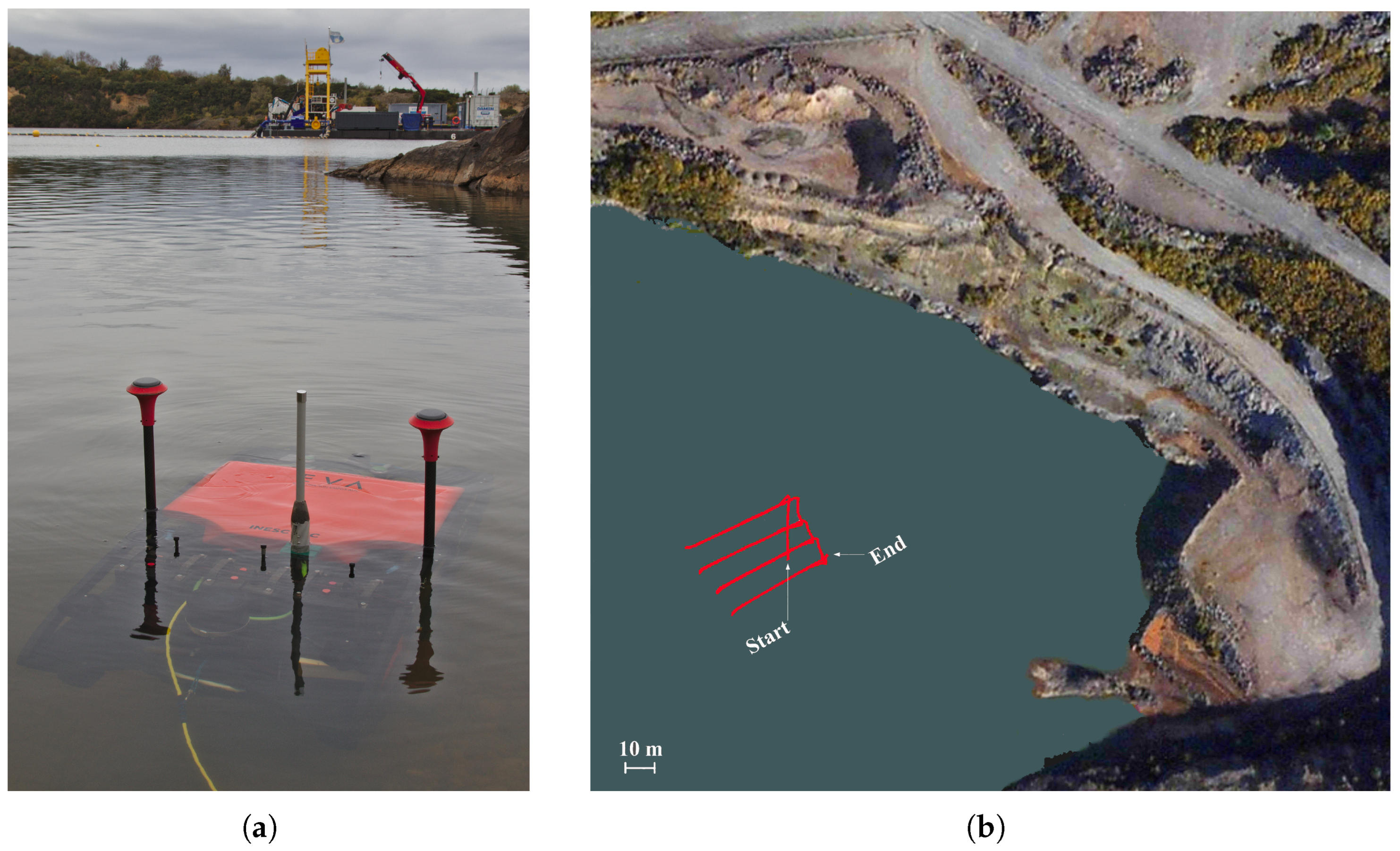
To validate the proposed method, we resort to a real dataset collected by the EVA AUV during the ¡VAMOS! project field tests, conducted at the Magcobar flooded quarry in the Silvermines district, Republic of Ireland (Figure 7a).

To ensure an accurate ground-truth, a trajectory segment where the AUV navigates on the surface, with continuous GNSS reception, was selected for testing. Through a dual-antenna GNSS receiver, and applying the real time kinematic (RTK) technique, precise position, linear velocity and heading measurements were obtained [6]. The reference trajectory was computed in real time onboard through a loosely coupled sensor fusion method, based on an Extended Kalman Filter (EKF). This fusion scheme integrates all GNSS observations with inertial data from a FOG IMU, bottom-referenced velocity measurements from a DVL, and depth estimates from a pressure sensor.

The trajectory segment was recorded over a 21 min survey, during which the AUV traversed approximately 276 m and mapped an area of about 2435 square m. The surveyed terrain comprises multiple stepped levels, known as benches, separated by steep vertical walls, referred to as bench faces. Since the Echoscope 3D sonar is slightly angled ahead, overlapping passes were executed in both directions to minimize occlusions in the vertical bench face regions. The resulting trajectory is depicted in Figure 7b.

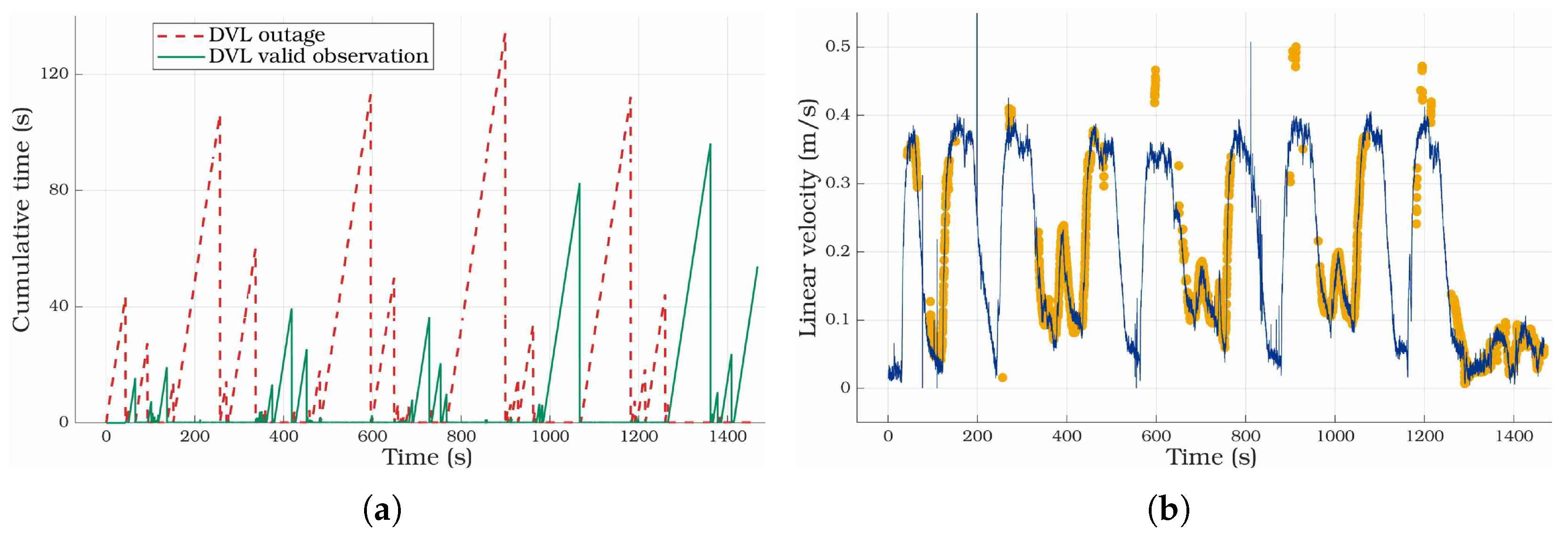
The dataset poses a significant challenge due to a DVL malfunction that limited valid velocity measurements to only about 30% of the total mission time. As shown in Figure 8a, the longest DVL outage persisted for 131 s, while the longest uninterrupted sequence of valid readings lasted 96 s. These prolonged interruptions prevented the DVL from accurately capturing major velocity variations, as illustrated in Figure 8b, where DVL derived linear velocity is compared against the GNSS reference. Under such conditions, state-of-the-art bathymetric SLAM methods that depend on submap construction are likely to fail, since submap consistency deteriorates rapidly when dead reckoning accuracy is compromised. This scenario provides an ideal test case for our approach, which, by avoiding submap creation, aims to still perform in situations of degraded dead reckoning.

Registering all incoming scans would introduce significant computational overhead due to repeated scan matching operations and the increased complexity of the SLAM factor graph. This overhead can be effectively mitigated, while ensuring reliable convergence without compromising registration accuracy, by restricting scan matching to a subset of key scans. In the original 3DupIC work [17], convergence experiments demonstrate high registration accuracy for relative displacements of up to approximately 3 m. Although convergence can still be achieved for scan overlaps of about 40%—corresponding to relative displacements of roughly 5 m when operating at an altitude of 10 m above the seafloor—the registration accuracy degrades beyond this regime. Furthermore, a temporal performance analysis presented in [63] confirms real-time scan matching capability when registering key scans separated by approximately 2 m, assuming linear vehicle motion at a speed of 2 m/s.

Based on these results, scan matching in this work is performed exclusively between key scans, which are selected either according to a minimum relative displacement of 2 m or a maximum elapsed time of 20 s since the last registration. The displacement criterion ensures distinct perspectives are captured while maintaining consistent registration, whereas the temporal criterion prevents excessive gaps during slow motion or changes in vehicle direction. Although these thresholds provide a favorable trade-off between registration accuracy, computational load, and SLAM graph scalability, they remain dependent on the operational environment, and may require adjustment to account for variations in terrain morphology, vehicle dynamics, sensor altitude, and available computational resources.

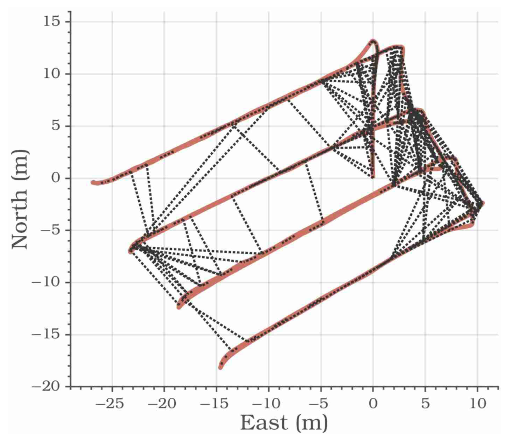
In this experiment, a total of 600 key scans were successfully registered using the 3DupIC algorithm, resulting in 599 factors relating consecutive poses and 268 loop-closure factors. Across this dataset, sonar ranges span from 16.85 m to 43.21 m. Loop-closures were performed between robot poses separated by distances ranging from 1.18 m to 36.15 m (Figure 9), demonstrating the algorithm’s ability to reconcile both short and long displacements.

6.2. Localization Results

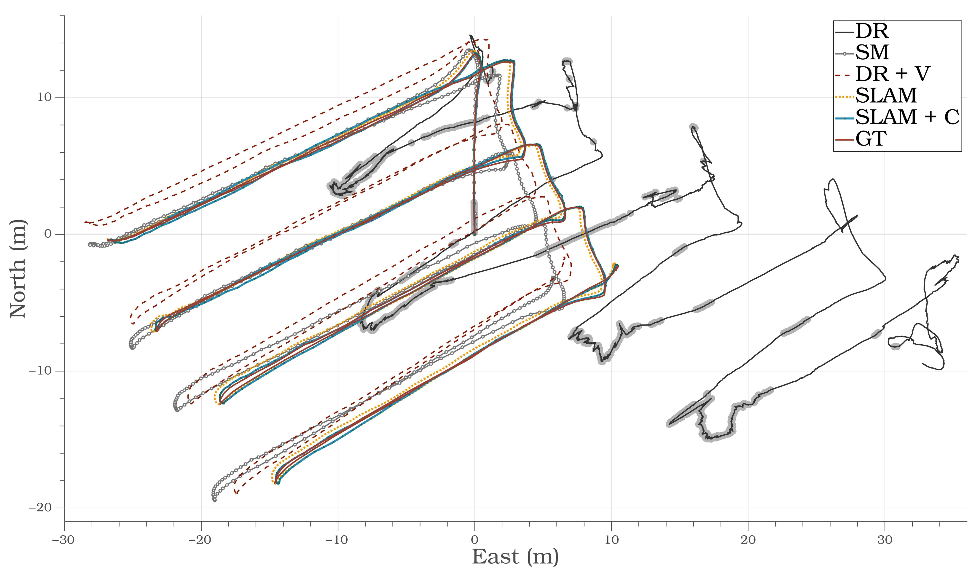
A direct comparison with the ground-truth trajectory (GT) is performed to evaluate localization performance. In addition to the proposed SLAM with calibration method (SLAM + C), Figure 10 and Figure 11 present the results obtained from intermediate methods such as dead reckoning (DR), scan matching (SM), dead reckoning with velocity initialization (DR + V) and SLAM without extrinsic calibration (SLAM). 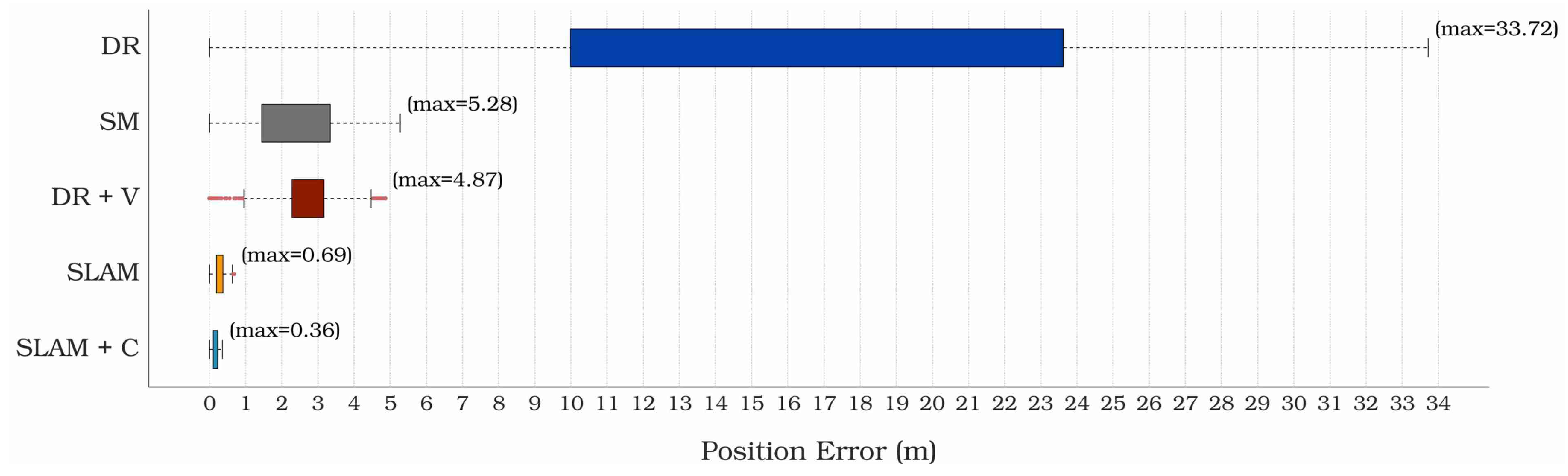Figure 10 depicts the trajectories produced by each method, while Figure 11 summarizes the corresponding position errors.

For the current test case, the dead reckoning based on DVL and gyroscopes yields the poorest performance. The rapid deviation from the ground-truth trajectory observed in Figure 10 is explained by the DVL’s inability to provide periodic velocity measurements. Without this information, the constant velocity model adopted in the EKF prediction step cannot reliably observe the AUV motion, reaching a maximum deviation of 33.72 m with respect to the ground-truth (Figure 11). It should be noted that this dead reckoning solution is not directly incorporated into the SLAM and calibration factor graph; it is only presented here to demonstrate the standalone performance of the method on the current dataset.

By transforming all displacement increments computed by the 3DupIC to the body frame and placing them together, trajectory labeled SM in Figure 10 is produced. When compared with the dead reckoning trajectory, the scan matching demonstrates a clear improvement in localization accuracy. With respect to the ground-truth, a noticeable drift, particularly affecting the orientation states, can be observed in Figure 10. This is justified by the fact that, appart from the initialization provided by dead reckoning, no information from the FOG gyroscopes is considered in this solution, as position and attitude are exclusivelly computed through sonar scan registration. Additionally, no loop-closures where established at this point and uncalibrated extrinsic parameters where used to transform displacements between the sonar and the body reference frames.

To mitigate the lack of reliable velocity measurements supplied to the dead reckoning system, velocity references obtained from scan matching are provided at the beginning of each trajectory segment, as detailed in Section 4.1. Displacements computed by this modified dead reckoning system are used to produce the dead reckoning factors in the SLAM and calibration factor graph. The performance of the modified dead reckoning is identified by the label DR + V in Figure 10 and Figure 11. When compared to the original dead reckoning approach, a significant improvement is achieved, with a reduction in position error by nearly an order of magnitude. When compared with the scan matching (SM), the DR + V trajectory exhibits a more consistent estimation of the vehicle’s orientation states, with the trajectory path showing better alignment with the ground-truth (GT), thanks to the inclusion of FOG gyroscopes. However, inaccuracies in velocity estimation still lead to large positioning errors, particularly noticeable during the first half of the mission, where DVL outages are more frequent (Figure 8).

The performance of the proposed graph-based SLAM approach is evaluated in two configurations: one with the extrinsic calibration component disabled (SLAM), and another with joint optimization of the trajectory and the extrinsic parameters (SLAM + C). Both configurations share the same factor graph structure, differing only in the uncertainty assigned to the extrinsic parameters. In the SLAM configuration, these parameters are tightly constrained with low prior uncertainty to prevent their modification during optimization, whereas in SLAM + C, a more relaxed constraint allows their refinement within the graph optimization process.

Both SLAM trajectories (Figure 10) show a substantial improvement over the previously presented methods, achieving approximately an order of magnitude gain in localization accuracy with respect to the SM and DR + V solutions (Figure 11). The SLAM + C configuration yields the most consistent and accurate results, with a maximum position error of 0.36 m relative to the ground-truth trajectory, while the SLAM solutions achieves a maximum error of 0.69 m. From a localization perspective, these results demonstrate the effectiveness of the proposed graph-SLAM formulation and highlight the added value of incorporating the ternary scan matching factor, which enables refinement of the transformation between reference frames. Ultimately, these figures clearly illustrate a progressive improvement in localization accuracy as the level of integration increases, reaching the best performance with the proposed SLAM and calibration method.

6.3. Mapping Results

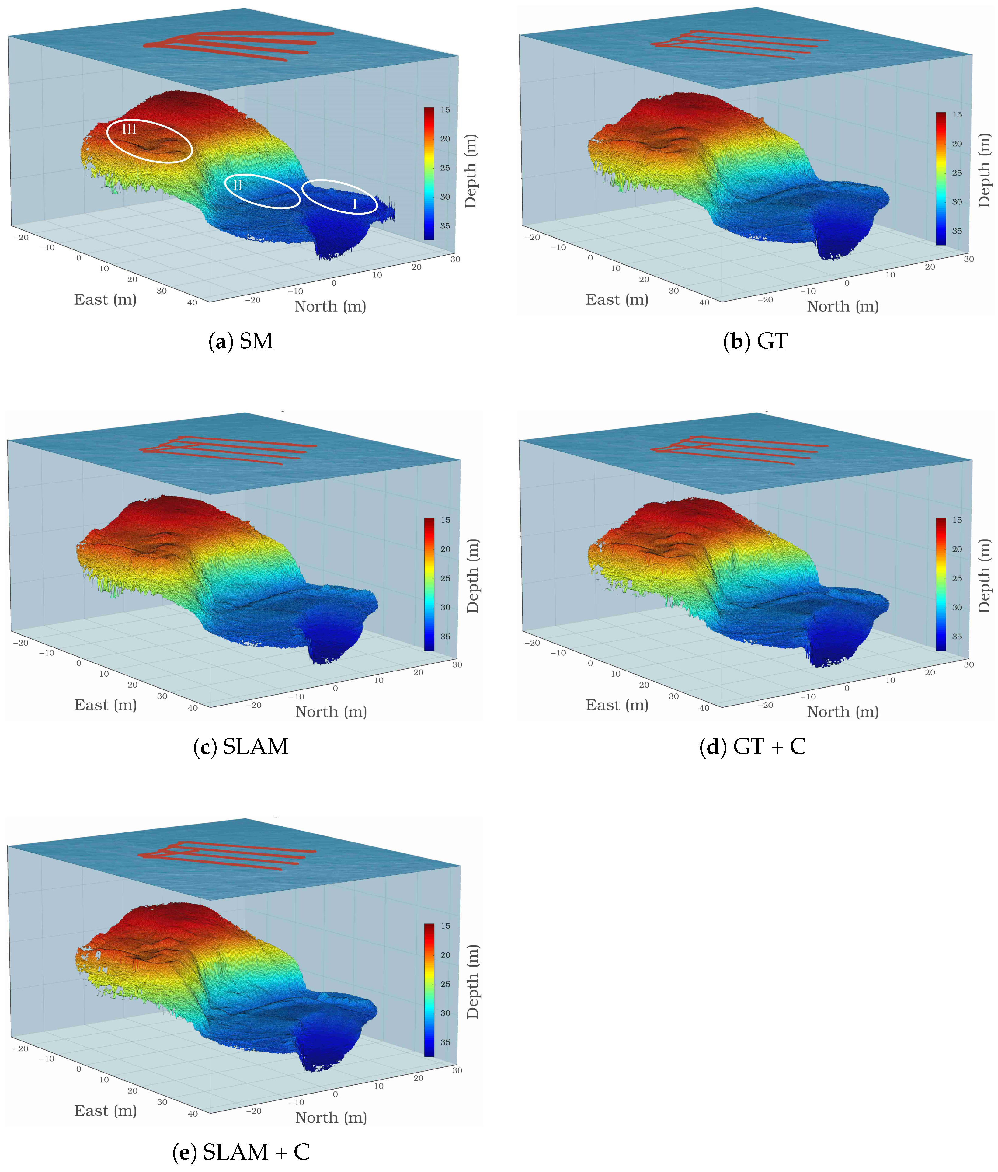
Based on the previously presented trajectories, the corresponding bathymetric models were constructed (Figure 12), allowing a visual assessment of the impact of each localization method on the consistency of the reconstructed surfaces. To generate these representations, point clouds were created by transforming the key scans into a common reference frame according to the poses estimated by each method. Subsequently, 2.5D elevation maps were computed, by discretizing the point clouds into a 20 × 20 cm grid cell and averaging the depth of the points contained within each cell.

Bathymetric maps were generated for the scan matching (SM), ground-truth (GT), SLAM, and SLAM + C trajectories (Figure 12). In the first three cases, the original extrinsic parameters were used to produce the point clouds whereas in the SLAM + C case, the refined parameters were applied. Additionally, an extra map, labeled GT + C, was constructed using the ground-truth trajectory combined with the refined extrinsic parameters estimated by the SLAM and calibration method. This configuration allows the effect of the extrinsic calibration to be analyzed independently from trajectory estimation errors. 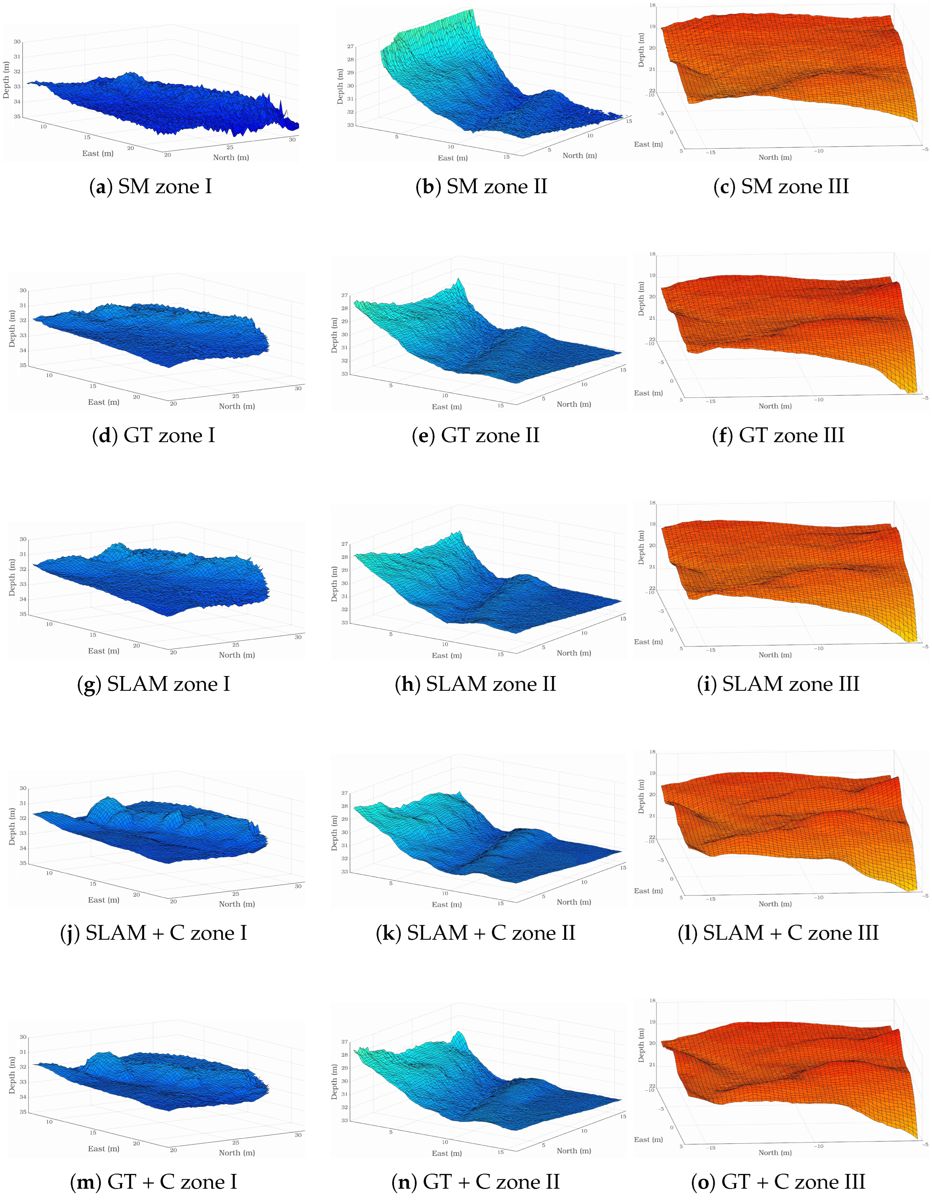From the models presented in Figure 12, close-up shots were extracted in three specific areas. This enlarged segments, depicted in Figure 13, facilitate the visual comparison between the different models.

All reconstructed models shown in Figure 12 successfully capture the general morphology of the surveyed underwater terrain, preserving the main topographic features. However, closer inspection reveals subtle geometric distortions and differences in surface definition between reconstructions. Maps reconstructed from less consistent trajectories—such as scan matching—tend to produce smoother surfaces. This apparent smoothness, however, does not indicate higher accuracy; rather, it results from the loss of fine geometric detail caused by local misalignments between overlapping scans. When scan alignment is poor, small scale features are effectively blurred out during the grid based averaging process, leading to an overly smoothed surface representation.

In contrast, the models generated using the SLAM and SLAM + C trajectories exhibit sharper and more coherent structures, reflecting improved spatial alignment between scans. The introduction of loop-closure constraints within the SLAM formulation mitigates long term drift, ensuring a globally consistent reconstruction. Furthermore, in the SLAM + C configuration, the joint optimization of extrinsic calibration refines the sonar to body transformation, enhancing local consistency and allowing finer structural details to emerge.

Surprisingly, the models reconstructed from the ground-truth trajectory do not offer the highest amount of detail. Nevertheless, when original extrinsic parameters are replaced by the refined ones, the reconstruction quality increases significantly and becomes close to the SLAM + C model. This outcome reveals the effectiveness of extrinsic parameter refinement within the SLAM factor graph. Nevertheless, since the calibration was performed jointly with the SLAM + C trajectory, the refined parameters are inherently adapted to the characteristics of that trajectory, which still contains residual errors relative to the ground-truth. Therefore, the fact that these parameters yield a slightly inferior reconstruction when applied to the ground-truth trajectory suggests that, while they provide a good fit to the SLAM + C trajectory, they still retain a certain degree of global uncertainty.

Close-up views presented in Figure 13 provide magnified visualizations of three selected regions for each reconstruction. Beyond the previously noted lack of detail in the scan matching solution, a low amplitude and high frequency noise superimposed on all surfaces becomes apparent. These local variations indicate inconsistencies between the depth stored in neighboring cells, once again suggesting poor scan alignment. The SLAM reconstruction demonstrates clear improvements in both surface clarity and structural definition, with most of the roughness observed in the scan matching model effectively corrected. The SLAM + C map stands out as the most consistent, revealing finer topographic details while maintaining smoothness in flat regions. The effectiveness of the SLAM and calibration factor graph in refining the sonar-to-body transformation is further confirmed by the significant improvement observed between the GT and the GT + C models.

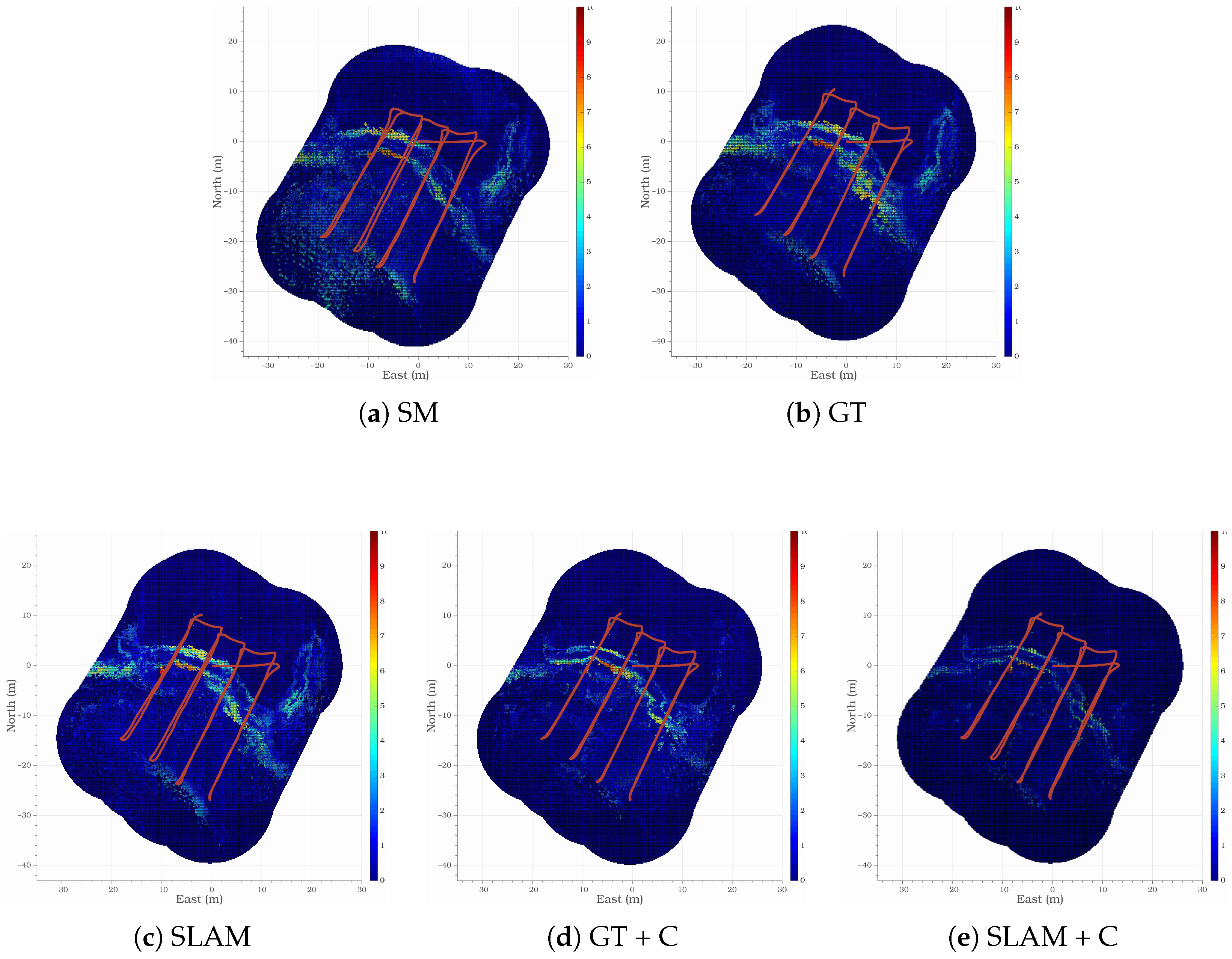
Finally, the self-consistency of each model was evaluated using the method described in [71], which quantifies, for each cell, the disparity among the contributing scans. A preliminary examination of the results shown in Figure 14 indicates that the largest errors occur in areas with steep slopes, where the terrain geometry naturally amplifies minor misalignment between scans. Also, in transition zones between different elevation levels, the metric may overestimate error, as a single cell can contain points originating from distinct height layers. In this context, the metric is not suitable for assessing a global error. Although it could be extended to a 3D voxel representation, a 2D grid discretization was adopted, as it still allows meaningful comparisons between methods while preserving visual clarity.

The error figures corroborate the empirical observations derived from Figure 12 and Figure 13. The scan matching map exhibits the worst performance, while the ground-truth based map performs slightly worse than the SLAM solution without calibration. The SLAM + C configuration demonstrates the highest consistency, showing reduced errors in flat regions and a sharper, more localized error response along terrain slopes. However, it should be noted that in these steep transition zones, the concentration of high error values may not necessarily reflect true reconstruction inaccuracies but rather the aggregation of depth measurements from different terrain levels within the same grid cell. This effect can artificially inflate the local error estimate while still indicating good overall alignment quality. Nevertheless, compared to the other reconstructions, the SLAM + C solution confines high error regions to narrower terrain bands, demonstrating superior internal consistency. The GT + C model also shows improved consistency compared to the non calibrated counterpart, further reinforcing the benefit of refined extrinsic calibration in achieving a coherent 3D reconstruction.

6.4. Calibration Results

This section evaluates the performance of the proposed extrinsic calibration approach, with particular emphasis on its convergence properties, robustness to poor initialization, and repeatability. The subsequent analyses investigate the response of the calibration method to initialization errors by introducing controlled perturbations in the prior factor ${\mathbf{z}}^{\mathbf{T}}$ associated with the extrinsic parameters. Perturbations are applied individually to each translational component $(x^{\mathbf{T}},y^{\mathbf{T}},z^{\mathbf{T}})$ and to each rotational component $({\varphi }^{\mathbf{T}},{\theta }^{\mathbf{T}},{\psi }^{\mathbf{T}})$, expressed as Euler angles.

All experiments are conducted using the same real-world dataset and the SLAM and calibration factor graph employed previously. The extrinsic parameters obtained from the batch optimization of the SLAM and calibration factor graph are used as reference values in all subsequent experiments.

6.4.1. Observability Analysis

This experiment aims to assess the observability of the individual extrinsic parameters within the proposed calibration framework by analyzing the convergence behavior under controlled perturbations applied independently to each degree of freedom. To this end, each parameter is perturbed in isolation while the remaining components are kept at their nominal values, allowing the evaluation of whether the constraints provided by the factor graph are sufficient to drive convergence towards the reference solution.

This test represents a worst case scenario, in which the imposed perturbations significantly exceed the uncertainty typically associated with preliminary extrinsic calibration obtained through manual measurements on the vehicle. This deliberate exaggeration is intended to evaluate the robustness of the method under adverse initialization conditions. Translational components were perturbed within a range of $\pm 0.5$ m around the reference values, sampled at regular intervals of 2 cm. Rotational components were perturbed within a range of $\pm 5°$, using increments of $0.2°$. These bounds and step sizes result in 100 tested samples for each individual parameter.

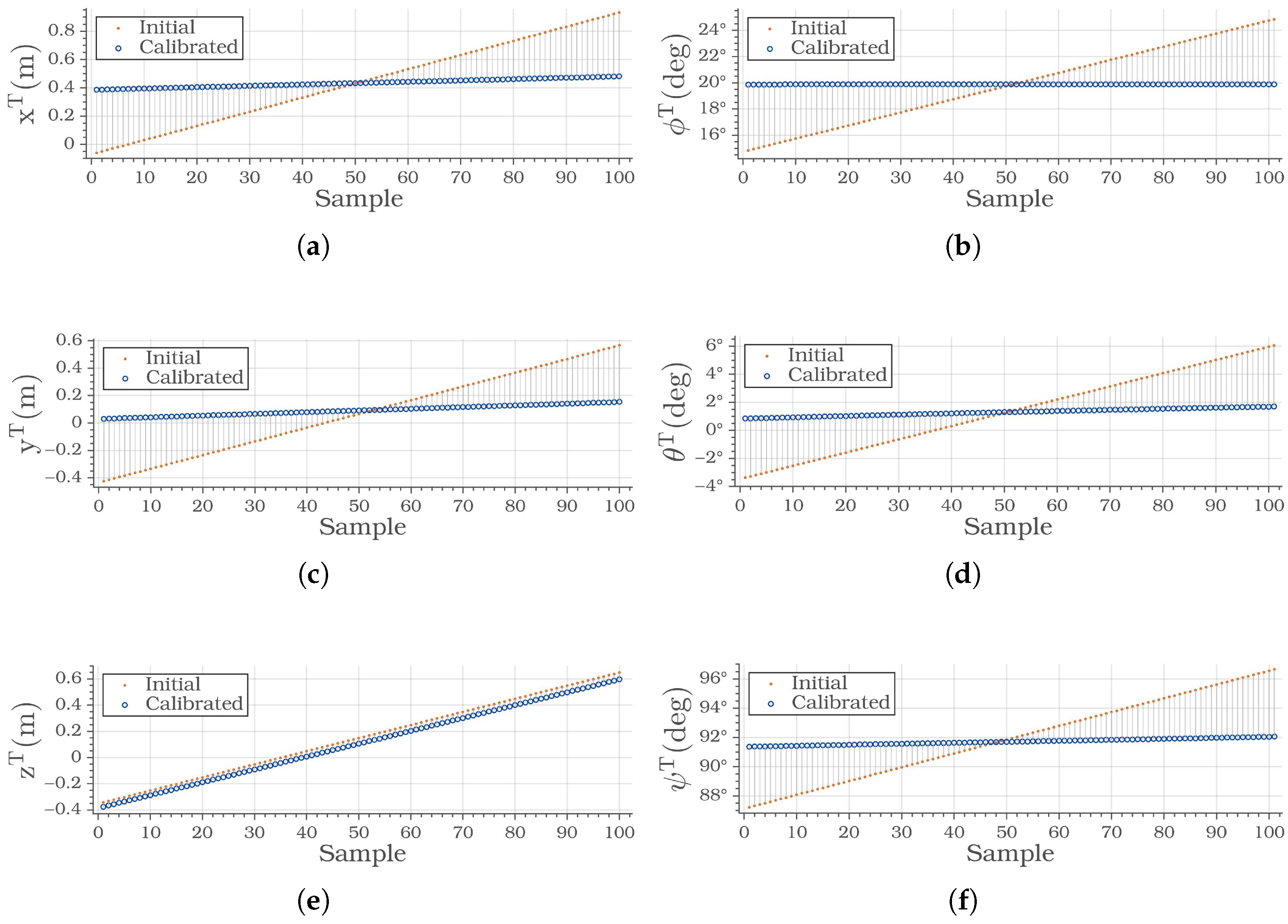
The resulting plots, shown in Figure 15, illustrate the response of the calibration method (blue circles) to variations in the initial extrinsic parameter values (orange markers). Each plot displays 100 samples, where the central sample (sample 50) represents an initial value close to the reference extrinsic parameter, while samples farther from the center correspond to progressively larger deviations from this reference.

Despite the large initialization errors, the proposed method exhibits consistent convergence, with the calibrated parameters approaching the reference values across most degrees of freedom. This trend is observed for all components except for the vertical translation component $z^{\mathbf{T}}$ (Figure 15e), whose calibrated values tend to follow the imposed perturbation.

The limited convergence observed for the vertical translation component $z^{\mathbf{T}}$ is attributed to reduced observability in the considered dataset. The environment is dominated by horizontal structures, and the vehicle exhibits very limited roll and pitch motion, which diminishes the sensitivity of scan matching constraints to vertical sensor offsets. As a result, this degree of freedom becomes weakly constrained in the factor graph and can be partially compensated by adjustments in the estimated trajectory.

6.4.2. Convergence and Geometric Consistency Analysis

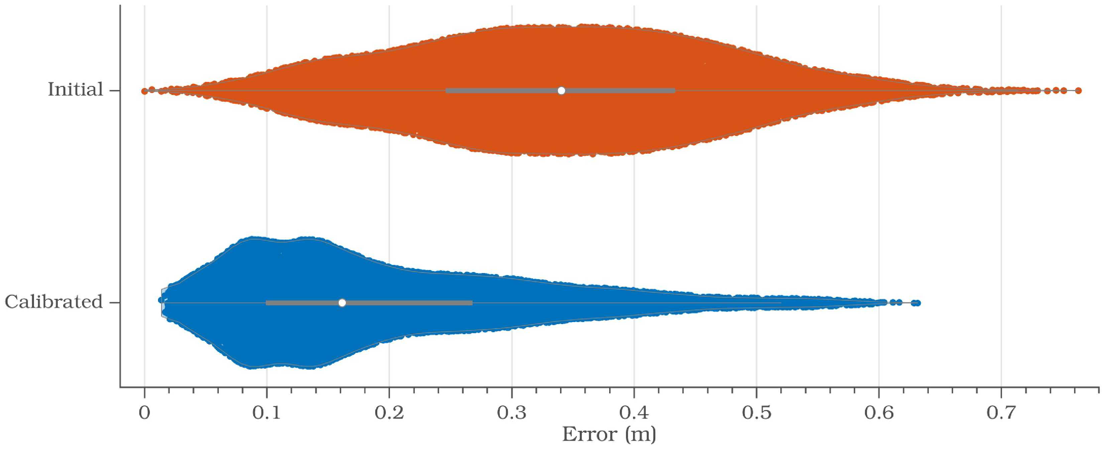
After evaluating the effect of poor initialization on each extrinsic parameter independently, a more realistic scenario is considered in which all components are perturbed simultaneously. In this experiment, smaller perturbations are introduced, consistent with the levels of uncertainty typically encountered in real-world deployments. Such uncertainties may arise from slight sensor mounting offsets, installation tolerances, minor structural deformations of the vehicle body, and imprecise initial measurements of the extrinsic parameters. Translational components are perturbed within $\pm 10$ cm using increments of 5 cm, while rotational components are perturbed within $\pm 1°$ using increments of $0.5°$. This results in a total of $5^6$ combinations, corresponding to 15,625 samples.

This experiment also serves to quantify the geometric impact of the extrinsic parameters on the transformation of sonar measurements between reference frames. For each sample, a point is randomly selected from a 3D scan acquired by the Echoscope 3D sonar and transformed from the sonar reference frame to the vehicle body frame. Three transformations are preformed: one using the perturbed initial extrinsic parameters, one using the calibrated parameters obtained after optimization, and one using the reference extrinsic parameters. For both the perturbed and calibrated cases, the projection error is computed as the Euclidean distance to the reference projection obtained with the reference extrinsic parameters. This metric provides a direct geometric measure of the misalignment induced by initialization errors and of the extent to which the calibration process corrects them.

The resulting distance distributions are summarized in the violin plots shown in Figure 16. A clear separation is observed between the distributions obtained with the perturbed initial parameters and those obtained after calibration. In particular, the median projection error associated with the calibrated parameters (0.158 cm) is less than half of that obtained with the perturbed parameters (0.34 cm), highlighting the effectiveness of the calibration process in reducing geometric misalignment.

Moreover, the calibrated parameters lead to a clear shift of the error distribution towards the origin, indicating that most scan points are projected with small residual errors after calibration. This marked reduction in both dispersion and bias demonstrates the convergence of the calibration process, but also its repeatability and stability across a large set of perturbation scenarios.

7. Discussion

Overall, the presented results demonstrate a clear and consistent improvement in both trajectory estimation and map reconstruction as the level of integration among localization methods increases. The progression from standalone approaches—such as dead reckoning and scan matching—to a fully integrated SLAM formulation leads to substantial gains in global consistency and positional accuracy. These results confirm that jointly exploiting complementary sources of relative and global constraints is essential for robust underwater localization.

The inclusion of extrinsic calibration within the SLAM optimization proves particularly beneficial. Beyond refining the transformation between the sonar and body frames, joint trajectory and calibration optimization improves scan alignment and enhances the geometric coherence of the reconstructed maps. Notably, the SLAM + C solution yields more consistent reconstructions than those obtained using the ground-truth trajectory. This outcome stems from the inherent coupling between trajectory estimation and extrinsic calibration: when optimized jointly, correlations between states can lead to cross-compensation effects and ambiguous error attribution, effectively binding both solutions together.

Nonetheless, applying the refined extrinsic parameters to the ground-truth trajectory also results in a noticeable improvement in reconstruction quality. This indicates that, although the calibrated parameters may not correspond to a globally exact solution, they approach the true values and provide tangible benefits when transferred across trajectories. The calibration convergence experiments further support this interpretation. In particular, the second experiment shown in Figure 16 reveals that no sample achieves zero projection error, even when re-initialized from previously calibrated parameters. This behavior suggests that the calibration problem is only partially observable, allowing the optimization to converge to slightly different local optima depending on initialization. This effect is consistent with the individual parameter analysis presented in Figure 15, and is especially evident in the vertical translational component, which exhibits the weakest observability.

Improved observability of the extrinsic parameters may require either a larger number of loop-closure constraints or more expressive vehicle motion. In particular, stronger excitation of the pitch and roll degrees of freedom could contribute to better constrain the extrinsic parameters. Despite this, the vertical translation component does not diverge during optimization. Instead, the calibrated value remains close to its initial estimate, indicating that while refinement is limited, the calibration process does not introduce instability or degradation.

The limited refinement of the vertical component primarily manifests as a small vertical offset in the reconstructed 3D model. However, when comparing the reconstructions in Figure 13, this offset is imperceptible due to the small magnitude of the adjustment (approximately 2.5 cm). As a result, the overall impact on mapping quality is negligible for the dataset considered.

To further improve calibration accuracy, especially along the vertical axis, the incorporation of additional absolute measurements into the factor graph can be considered. In particular, global position updates from a GNSS system expressed in the body frame could help constrain the vehicle pose, while depth measurements from a pressure sensor could be directly associated with the sonar frame. Such constraints would strengthen vertical observability and improve the conditioning of this degree of freedom, leading to more accurate and fully observable extrinsic calibration.

8. Conclusions

This work proposes a pose-graph SLAM and calibration framework built upon the 3DupIC probabilistic scan matching algorithm. The proposed system demonstrates strong robustness to degraded dead reckoning conditions, as it does not depend on submap construction. Instead, by registering consecutive key scans together, the 3DupIC provides an alternative odometry estimate, which is used to aid the dead reckoning system. Experimental results demonstrate remarkable performance in both localization and mapping accuracy.

Another key contribution lies in the inclusion of an additional node within the factor graph to represent the sonar-to-body transformation. These extrinsic parameters are connected through scan matching factors, enabling their accurate estimation within the global SLAM optimization process. The experimental analysis demonstrates consistent convergence and repeatability of the calibration process, even under significant initialization errors, while also revealing the influence of observability and vehicle motion on specific parameters. Future developments will focus on improving parameter observability, particularly along the vertical component, through enhanced sensor fusion. Finally, a deeper analysis of the relationship between the number of loop-closure factors and the accuracy of extrinsic parameter estimation remains to be conducted.

Additionally, future validation should consider larger-scale datasets involving longer trajectories and, consequently, higher levels of accumulated drift. Such scenarios will require an improved loop-closure detection strategy, as the current approach—based solely on spatial proximity between scans—may become less effective as temporal separation and drift increase. Under these conditions, strategies that exploit the intrinsic content of the scans, such as feature extraction, scan descriptor construction, or other place recognition techniques, may contribute to more reliable loop-closure detection.

Scan-matching systems, which seek to establish correspondences between scans based on the underlying morphology, inherently benefit from environments that are structurally rich and diverse. The proposed method has demonstrated its effectiveness in such a setting; however, its ability to generalize to smoother and less structured environments, which often characterize the seabed, will need to be assessed in future work.

The calibration process benefits from considering all available information simultaneously. For this reason, the current implementation operates offline, building the entire factor graph first and then performing graph optimization to obtain both trajectory and calibrated extrinsic. However, extrinsic calibration is only required occasionally, whenever the sonar mounting changes. From an operational standpoint, the proposed framework could be further developed into an incremental SLAM system, capable of performing online optimization as the vehicle explores the environment and progressively establishes loop-closures. The current GPU based implementation of the 3DupIC algorithm already ensures real time scan matching performance, providing the necessary foundation for such an online SLAM deployment.

This study highlights how 3D profiling sonars can contribute to improve accuracy and consistency of underwater localization and mapping systems. The growing availability of compact and cost-effective 3D sonars makes this approach particularly pertinent. As these sensors become more accessible, their integration is expected to play a key role in enabling more accurate, autonomous, and efficient underwater robotic systems.

References

- Petillot, Y.R.; Antonelli, G.; Casalino, G.; Ferreira, F. Underwater Robots: From Remotely Operated Vehicles to Intervention-Autonomous Underwater Vehicles. IEEE Robot. Autom. Mag. 2019, 26, 94–101. [Google Scholar] [CrossRef]
- Zhang, B.; Ji, D.; Liu, S.; Zhu, X.; Xu, W. Autonomous Underwater Vehicle navigation: A review. Ocean Eng. 2023, 273, 113861. [Google Scholar] [CrossRef]
- Vallicrosa, G.; Himri, K.; Ridao, P.; Gracias, N. Semantic Mapping for Autonomous Subsea Intervention. Sensors 2021, 21, 6740. [Google Scholar] [CrossRef]
- Aulinas, J.; Petillot, Y.; Salvi, J.; Lladó, X. The SLAM Problem: A Survey. In Conference on Artificial Intelligence Research and Development: Proceedings of the 11th International Conference of the Catalan Association for Artificial Intelligence; IOS Press: Amsterdam, The Netherlands, 2008; pp. 363–371. [Google Scholar]
- McConnell, J.; Collado-Gonzalez, I.; Englot, B. Perception for Underwater Robots. Curr. Robot. Rep. 2022, 3, 177–186. [Google Scholar] [CrossRef]
- Ferreira, A.; Matias, B.; Almeida, J.; Silva, E. Real-time GNSS precise positioning: RTKLIB for ROS. Int. J. Adv. Robot. Syst. 2020, 17, 1729881420904526. [Google Scholar] [CrossRef]
- Almeida, J.; Ferreira, A.; Matias, B.; Lomba, C.; Martins, A.; Silva, E. ¡VAMOS! Underwater Mining Machine Navigation System. In Proceedings of the 2018 IEEE/RSJ International Conference on Intelligent Robots and Systems (IROS), Madrid, Spain, 1–5 October 2018; IEEE: Piscataway, NJ, USA, 2018; pp. 1520–1526. [Google Scholar] [CrossRef]
- Rypkema, N.R.; Singh, K. Hybrid Long/Inverted Ultra-Short Baseline (LBL-iUSBL) Acoustic Pose Estimation for Underwater Sonar Mapping. IEEE J. Ocean. Eng. 2025, 50, 1616–1625. [Google Scholar] [CrossRef]
- Almeida, J.; Matias, B.; Ferreira, A.; Almeida, C.; Martins, A.; Silva, E. Underwater Localization System Combining iUSBL with Dynamic SBL in ¡VAMOS! Trials. Sensors 2020, 20, 4710. [Google Scholar] [CrossRef] [PubMed]
- Macario Barros, A.; Michel, M.; Moline, Y.; Corre, G.; Carrel, F. A Comprehensive Survey of Visual SLAM Algorithms. Robotics 2022, 11, 24. [Google Scholar] [CrossRef]
- Wang, X.; Fan, X.; Shi, P.; Ni, J.; Zhou, Z. An Overview of Key SLAM Technologies for Underwater Scenes. Remote Sens. 2023, 15, 2496. [Google Scholar] [CrossRef]
- Zhang, S.; Zhao, S.; An, D.; Liu, J.; Wang, H.; Feng, Y.; Li, D.; Zhao, R. Visual SLAM for underwater vehicles: A survey. Comput. Sci. Rev. 2022, 46, 100510. [Google Scholar] [CrossRef]
- Heshmat, M.; Saad Saoud, L.; Abujabal, M.; Sultan, A.; Elmezain, M.; Seneviratne, L.; Hussain, I. Underwater SLAM Meets Deep Learning: Challenges, Multi-Sensor Integration, and Future Directions. Sensors 2025, 25, 3258. [Google Scholar] [CrossRef]
- Vallicrosa, G.; Ridao, P. H-SLAM: Rao-Blackwellized Particle Filter SLAM Using Hilbert Maps. Sensors 2018, 18, 1386. [Google Scholar] [CrossRef]
- Hansen, R.K.; Andersen, P.A. A 3D Underwater Acoustic Camera—Properties and Applications. In Acoustical Imaging; Springer: Boston, MA, USA, 1996; pp. 607–611. [Google Scholar] [CrossRef]
- Martins, A.; Almeida, J.; Almeida, C.; Matias, B.; Kapusniak, S.; Silva, E. EVA a Hybrid ROV/AUV for Underwater Mining Operations Support. In Proceedings of the 2018 OCEANS—MTS/IEEE Kobe Techno-Oceans (OTO), Kobe, Japan, 28–31 May 2018; IEEE: Piscataway, NJ, USA, 2018; pp. 1–7. [Google Scholar] [CrossRef]
- Ferreira, A.; Almeida, J.; Martins, A.; Matos, A.; Silva, E. 3DupIC: An Underwater Scan Matching Method for Three-Dimensional Sonar Registration. Sensors 2022, 22, 3631. [Google Scholar] [CrossRef] [PubMed]
- Williams, S.; Newman, P.; Dissanayake, G.; Durrant-Whyte, H. Autonomous underwater simultaneous localisation and map building. In Proceedings of the 2000 ICRA, Millennium Conference, IEEE International Conference on Robotics and Automation, Symposia Proceedings (Cat. No.00CH37065), San Francisco, CA, USA, 24–28 April 2000; IEEE: Piscataway, NJ, USA, 2000; Volume 2, pp. 1793–1798. [Google Scholar] [CrossRef]
- Ribas, D.; Ridao, P.; Tardós, J.D.; Neira, J. Underwater SLAM in man-made structured environments. J. Field Robot. 2008, 25, 898–921. [Google Scholar] [CrossRef]
- González, Y.; Oliver, G.; Burguera, A. Underwater Scan Matching using a Mechanical Scanned Imaging Sonar. IFAC Proc. Vol. 2010, 43, 377–382. [Google Scholar] [CrossRef]
- Chen, L.; Wang, S.; Hu, H.; Gu, D.; Liao, L. Improving Localization Accuracy for an Underwater Robot with a Slow-Sampling Sonar Through Graph Optimization. IEEE Sens. J. 2015, 15, 5024–5035. [Google Scholar] [CrossRef]
- Johannsson, H.; Kaess, M.; Englot, B.; Hover, F.; Leonard, J. Imaging sonar-aided navigation for autonomous underwater harbor surveillance. In Proceedings of the 2010 IEEE/RSJ International Conference on Intelligent Robots and Systems, Taipei, Taiwan, 18–22 October 2010; IEEE: Piscataway, NJ, USA, 2010; pp. 4396–4403. [Google Scholar] [CrossRef]
- Negahdaripour, S. On 3-D Motion Estimation From Feature Tracks in 2-D FS Sonar Video. IEEE Trans. Robot. 2013, 29, 1016–1030. [Google Scholar] [CrossRef]
- Huang, T.A.; Kaess, M. Towards acoustic structure from motion for imaging sonar. In Proceedings of the 2015 IEEE/RSJ International Conference on Intelligent Robots and Systems (IROS), Hamburg, Germany, 28 September–3 October 2015; IEEE: Piscataway, NJ, USA, 2015; pp. 758–765. [Google Scholar] [CrossRef]
- Li, J.; Kaess, M.; Eustice, R.M.; Johnson-Roberson, M. Pose-Graph SLAM Using Forward-Looking Sonar. IEEE Robot. Autom. Lett. 2018, 3, 2330–2337. [Google Scholar] [CrossRef]
- McConnell, J.; Collado-Gonzalez, I.; Szenher, P.; Englot, B. Large-Scale Dense 3-D Mapping Using Submaps Derived From Orthogonal Imaging Sonars. IEEE J. Ocean. Eng. 2025, 50, 354–369. [Google Scholar] [CrossRef]
- Melo, J.; Matos, A. Survey on advances on terrain based navigation for autonomous underwater vehicles. Ocean Eng. 2017, 139, 250–264. [Google Scholar] [CrossRef]
- Fairfield, N.; Kantor, G.; Wettergreen, D. Real-Time SLAM with Octree Evidence Grids for Exploration in Underwater Tunnels. J. Field Robot. 2007, 24, 3–21. [Google Scholar] [CrossRef]
- Montemerlo, M.; Thrun, S.; Koller, D.; Wegbreit, B. FastSLAM: A factored solution to the simultaneous localization and mapping problem. In Proceedings of the Eighteenth National Conference on Artificial Intelligence, Edmonton, AB, Canada, 28 July–1 August 2002; American Association for Artificial Intelligence: Menlo Park, CA, USA, 2002; pp. 593–598. [Google Scholar]
- Durrant-Whyte, H.; Bailey, T. Simultaneous localization and mapping: Part I. IEEE Robot. Autom. Mag. 2006, 13, 99–110. [Google Scholar] [CrossRef]
- Barkby, S.; Williams, S.B.; Pizarro, O.; Jakuba, M.V. A featureless approach to efficient bathymetric SLAM using distributed particle mapping. J. Field Robot. 2011, 28, 19–39. [Google Scholar] [CrossRef]
- Barkby, S.; Williams, S.B.; Pizarro, O.; Jakuba, M.V. Bathymetric particle filter SLAM using trajectory maps. Int. J. Robot. Res. 2012, 31, 1409–1430. [Google Scholar] [CrossRef]
- Zhang, Q.; Li, Y.; Ma, T.; Cong, Z.; Zhang, W. Bathymetric Particle Filter SLAM with Graph-Based Trajectory Update Method. IEEE Access 2021, 9, 85464–85475. [Google Scholar] [CrossRef]
- Norgren, P.; Skjetne, R. A Multibeam-Based SLAM Algorithm for Iceberg Mapping Using AUVs. IEEE Access 2018, 6, 26318–26337. [Google Scholar] [CrossRef]
- Torroba, I.; Cella, M.; Terán, A.; Rolleberg, N.; Folkesson, J. Online Stochastic Variational Gaussian Process Mapping for Large-Scale Bathymetric SLAM in Real Time. IEEE Robot. Autom. Lett. 2023, 8, 3150–3157. [Google Scholar] [CrossRef]
- Eliazar, A.; Parr, R. DP-SLAM: Fast, Robust Simultaneous Localization and Mapping Without Predetermined Landmarks. In Proceedings of the 18th International Joint Conference on Artificial Intelligence, Acapulco, Mexico, 9–15 August 2003; Morgan Kaufmann Publishers Inc.: San Francisco, CA, USA, 2003; pp. 1135–1142. [Google Scholar]
- Fairfield, N.; Wettergreen, D. Evidence grid-based methods for 3D map matching. In Proceedings of the 2009 IEEE International Conference on Robotics and Automation, Kobe, Japan, 12–17 May 2009; IEEE: Piscataway, NJ, USA, 2009; pp. 1637–1642. [Google Scholar] [CrossRef]
- Montemerlo, M.; Thrun, S.; Roller, D.; Wegbreit, B. FastSLAM 2.0: An improved particle filtering algorithm for simultaneous localization and mapping that provably converges. In Proceedings of the 18th International Joint Conference on Artificial Intelligence, IJCAI’03, San Francisco, CA, USA, 9–15 August 2003; Morgan Kaufmann Publishers Inc.: San Francisco, CA, USA, 2003; pp. 1151–1156. [Google Scholar]
- Grisetti, G.; Stachniss, C.; Burgard, W. Improving Grid-based SLAM with Rao-Blackwellized Particle Filters By Adaptive Proposals and Selective Resampling. In Proceedings of the 2005 IEEE International Conference on Robotics and Automation, Barcelona, Spain, 18–22 April 2005; IEEE: Piscataway, NJ, USA, 2005; pp. 2432–2437. [Google Scholar] [CrossRef]
- Grisetti, G.; Stachniss, C.; Burgard, W. Improved Techniques for Grid Mapping with Rao-Blackwellized Particle Filters. IEEE Trans. Robot. 2007, 23, 34–46. [Google Scholar] [CrossRef]
- Zandara, S.; Ridao, P.; Ribas, D.; Mallios, A.; Palomer, A. Probabilistic surface matching for bathymetry based SLAM. In Proceedings of the 2013 IEEE International Conference on Robotics and Automation, Karlsruhe, Germany, 6–10 May 2013; IEEE: Piscataway, NJ, USA, 2013; pp. 40–45. [Google Scholar] [CrossRef]
- Palomer, A.; Ridao, P.; Ribas, D. Multibeam 3D Underwater SLAM with Probabilistic Registration. Sensors 2016, 16, 560. [Google Scholar] [CrossRef] [PubMed]
- Roman, C.; Singh, H. Improved vehicle based multibeam bathymetry using sub-maps and SLAM. In Proceedings of the 2005 IEEE/RSJ International Conference on Intelligent Robots and Systems, Edmonton, AB, Canada, 2–6 August 2005; IEEE: Piscataway, NJ, USA, 2005; pp. 3662–3669. [Google Scholar]
- Roman, C.; Singh, H. A Self-Consistent Bathymetric Mapping Algorithm. J. Field Robot. 2007, 24, 23–50. [Google Scholar] [CrossRef]
- Cadena, C.; Carlone, L.; Carrillo, H.; Latif, Y.; Scaramuzza, D.; Neira, J.; Reid, I.; Leonard, J.J. Past, Present, and Future of Simultaneous Localization and Mapping: Toward the Robust-Perception Age. IEEE Trans. Robot. 2016, 32, 1309–1332. [Google Scholar] [CrossRef]
- Grisetti, G.; Kümmerle, R.; Stachniss, C.; Burgard, W. A Tutorial on Graph-Based SLAM. IEEE Intell. Transp. Syst. Mag. 2010, 2, 31–43. [Google Scholar] [CrossRef]
- Dellaert, F. Factor Graphs: Exploiting Structure in Robotics. Annu. Rev. Control. Robot. Auton. Syst. 2021, 4, 141–166. [Google Scholar] [CrossRef]
- Torroba, I.; Bore, N.; Folkesson, J. Towards Autonomous Industrial-Scale Bathymetric Surveying. In Proceedings of the 2019 IEEE/RSJ International Conference on Intelligent Robots and Systems (IROS), Macau, China, 3–8 November 2019; IEEE: Piscataway, NJ, USA, 2019; pp. 6377–6382. [Google Scholar] [CrossRef]
- Bichucher, V.; Walls, J.M.; Ozog, P.; Skinner, K.A.; Eustice, R.M. Bathymetric factor graph SLAM with sparse point cloud alignment. In Proceedings of the OCEANS 2015—MTS/IEEE Washington, Washington, DC, USA, 19–22 October 2015; IEEE: Piscataway, NJ, USA, 2015; pp. 1–7. [Google Scholar] [CrossRef]
- Bore, N.; Torroba, I.; Folkesson, J. Sparse Gaussian Process SLAM, Storage and Filtering for AUV Multibeam Bathymetry. In Proceedings of the 2018 IEEE/OES Autonomous Underwater Vehicle Workshop (AUV), Porto, Portugal, 6–9 November 2018; IEEE: Piscataway, NJ, USA, 2018; pp. 1–6. [Google Scholar] [CrossRef]
- Vial, P.; Palomeras, N.; Solà, J.; Carreras, M. Underwater Pose SLAM using GMM scan matching for a mechanical profiling sonar. J. Field Robot. 2024, 41, 511–538. [Google Scholar] [CrossRef]
- Besl, P.; McKay, N.D. A method for registration of 3-D shapes. IEEE Trans. Pattern Anal. Mach. Intell. 1992, 14, 239–256. [Google Scholar] [CrossRef]
- Castellani, U.; Fusiello, A.; Murino, V.; Papaleo, L.; Puppo, E.; Pittore, M. A complete system for on-line 3D modelling from acoustic images. Signal Process. Image Commun. 2005, 20, 832–852. [Google Scholar] [CrossRef]
- Zhang, J.; Yao, Y.; Deng, B. Fast and Robust Iterative Closest Point. IEEE Trans. Pattern Anal. Mach. Intell. 2021, 44, 3450–3466. [Google Scholar] [CrossRef]
- Torroba, I.; Bore, N.; Folkesson, J. A Comparison of Submap Registration Methods for Multibeam Bathymetric Mapping. In Proceedings of the 2018 IEEE/OES Autonomous Underwater Vehicle Workshop (AUV), Porto, Portugal, 6–9 November 2018; IEEE: Piscataway, NJ, USA, 2018; pp. 1–6. [Google Scholar] [CrossRef]
- Ma, T.; Ding, S.; Li, Y.; Fan, J. A review of terrain aided navigation for underwater vehicles. Ocean Eng. 2023, 281, 114779. [Google Scholar] [CrossRef]
- Burguera, A.; Gonzalez, Y.; Oliver, G. Probabilistic Sonar Scan Matching for Robust Localization. In Proceedings of the 2007 IEEE International Conference on Robotics and Automation, Rome, Italy, 10–14 April 2007; IEEE: Piscataway, NJ, USA, 2007; pp. 3154–3160. [Google Scholar] [CrossRef]
- Montesano, L.; Minguez, J.; Montano, L. Probabilistic scan matching for motion estimation in unstructured environments. In Proceedings of the 2005 IEEE/RSJ International Conference on Intelligent Robots and Systems, Edmonton, AB, Canada, 2–6 August 2005; IEEE: Piscataway, NJ, USA, 2005; pp. 3499–3504. [Google Scholar] [CrossRef]
- Hernández, E.; Ridao, P.; Romagós, D.; Joan, B. MSISpIC: A Probabilistic Scan Matching Algorithm Using a Mechanical Scanned Imaging Sonar. J. Phys. Agents 2009, 3, 3–11. [Google Scholar] [CrossRef]
- Mallios, A.; Ridao, P.; Hernandez, E.; Ribas, D.; Maurelli, F.; Petillot, Y. Pose-based SLAM with probabilistic scan matching algorithm using a mechanical scanned imaging sonar. In Proceedings of the OCEANS 2009-EUROPE, Bremen, Germany, 11–14 May 2009; IEEE: Piscataway, NJ, USA, 2009; pp. 1–6. [Google Scholar] [CrossRef]
- Burguera, A.; Oliver, G.; Gonzàlez, Y. Scan-based SLAM with trajectory correction in underwater environments. In Proceedings of the 2010 IEEE/RSJ International Conference on Intelligent Robots and Systems, Taipei, Taiwan, 18–22 October 2010; IEEE: Piscataway, NJ, USA, 2010; pp. 2546–2551. [Google Scholar] [CrossRef]
- Palomer, A.; Ridao, P.; Ribas, D.; Mallios, A.; Gracias, N.; Vallicrosa, G. Bathymetry-based SLAM with difference of normals point-cloud subsampling and probabilistic ICP registration. In Proceedings of the 2013 MTS/IEEE OCEANS, Bergen, Norway, 10–14 June 2013; IEEE: Piscataway, NJ, USA, 2013; pp. 1–8. [Google Scholar] [CrossRef]
- Ferreira, A.; Almeida, J.; Matos, A.; Silva, E. Real-Time Registration of 3D Underwater Sonar Scans. Robotics 2025, 14, 13. [Google Scholar] [CrossRef]
- Chaves, S.M.; Galceran, E.; Ozog, P.; Walls, J.M.; Eustice, R.M. Pose-Graph SLAM for Underwater Navigation. In Sensing and Control for Autonomous Vehicles: Applications to Land, Water and Air Vehicles; Springer International Publishing: Cham, Switzerland, 2017; pp. 143–160. [Google Scholar] [CrossRef]
- Dellaert, F. Factor Graphs and GTSAM: A Hands-on Introduction; Georgia Institute of Technology: Atlanta, GE, USA, 2012. [Google Scholar]
- Kümmerle, R.; Grisetti, G.; Strasdat, H.; Konolige, K.; Burgard, W. G2o: A general framework for graph optimization. In Proceedings of the 2011 IEEE International Conference on Robotics and Automation, Shanghai, China, 9–13 May 2011; IEEE: Piscataway, NJ, USA, 2011; pp. 3607–3613. [Google Scholar] [CrossRef]
- Agarwal, S.; Mierle, K.; Team, T.C.S. Ceres Solver. 2023. Available online: https://github.com/ceres-solver/ceres-solver (accessed on 1 February 2026).
- Solà, J. Course on SLAM; Technical Report IRI-TR-16-04; Institut de Robòtica i Informàtica Industrial, CSIC-UPC: Barcelona, Spain, 2017. [Google Scholar]
- Dellaert, F.; Kaess, M. Square Root SAM: Simultaneous Localization and Mapping via Square Root Information Smoothing. Int. J. Robot. Res. 2006, 25, 1181–1203. [Google Scholar] [CrossRef]
- Solà, J.; Deray, J.; Atchuthan, D. A micro Lie theory for state estimation in robotics. arXiv 2021, arXiv:1812.01537. [Google Scholar] [CrossRef]
- Roman, C.; Singh, H. Consistency based error evaluation for deep sea bathymetric mapping with robotic vehicles. In Proceedings of the 2006 IEEE International Conference on Robotics and Automation, ICRA, Orlando, FL, USA, 15–19 May 2006; IEEE: Piscataway, NJ, USA, 2006; pp. 3568–3574. [Google Scholar] [CrossRef]
Figure 1.
Illustration of one scan obtained by the Echoscope 3D sonar mounted onboard the EVA AUV. The image shows two perspectives of the same scan: (a) top-left and (b) left side views. In addition to the scan points (red dots), the 3D model of the EVA AUV is also depicted. The sonar field of view, with 50 degrees aperture in both along-track and across-track directions, is sketched on the left image. As depicted in the right image, the Echoscope was mounted with a 20-degree tilt to prioritize the inspection of the area in front of the robot.
Figure 2.
Relation between two consecutive poses of the EVA AUV. A dead reckoning displacement estimate tracks the body frame displacement. The 3DupIC scan matching method provides a displacement measurement defined in the sonar reference frame s. The transformation represents the transformation from the body to the sonar reference frame. The global pose of the AUV is defined in the global world reference frame w.
Figure 3.
Factor graph structure representing the formulation of the SLAM and extrinsic calibration problems.
Figure 4.
High level architecture of the proposed front-end algorithm for building the SLAM and calibration factor graph.
Figure 5.
Velocity initialization using the scan matching solution from the previous trajectory segment.
Figure 6.
Illustration of the conical beam model adopted to construct the probabilistic representation of each scan point. In the figure, the beam aperture is deliberately exaggerated to improve visualization and interpretation.
Figure 7.
Dataset acquisition in the Magcobar mine during the ¡VAMOS! project field trials. (a) Photograph of the EVA AUV (foreground) also showing the Launch and Recovery Vessel (background). (b) Map representation of the trajectory followed by EVA during dataset acquisition.
Figure 8.
Evaluation of DVL performance: (a) temporal distribution of DVL outages, expressed as cumulative DVL failure time (red line) and cumulative time of valid measurements (green line); (b) comparison between DVL measured linear velocity (yellow dots) and GNSS-derived velocity (blue line).
Figure 9.
Planar view of the ground-truth trajectory (light solid line), with dotted lines indicating pose pairs connected by loop-closure constraints.
Figure 10.
Top view of the estimated trajectories obtained using the different localization approaches. Light gray dots superimposed on the dead reckoning (DR) trajectory indicate time instants with valid DVL velocity measurements.
Figure 11.
Position errors for the different methods, computed as the L2 norm with respect to the ground-truth.
Figure 12.
Bathymetric reconstructions obtained from different localization solutions: (
a) Scan Matching, (
b) ground-truth, (
c) SLAM, (
d) ground-truth with extrinsic calibration, (
e) SLAM and calibration. The areas highlighted in white in (
a) are shown magnified for all methods in
Figure 13.
Close-up views of bathymetric reconstructions obtained using different trajectories. The zoomed areas, indicated in
Figure 12, correspond to three selected regions of interest. Each column represents one of these areas, while each row corresponds to a different reconstruction method, enabling a detailed visual comparison of reconstruction accuracy and surface consistency across methods.
Figure 14.
Self-consistency error map computed over a 20 cm grid, illustrating local disparities among overlapping sonar scans for each reconstruction: (a) scan matching, (b) ground-truth, (c) SLAM, (d) ground-truth with refined extrinsic parameters, (e) SLAM with calibration. The corresponding robot trajectories are superimposed in red, indicating the vehicle path associated with each reconstruction.
Figure 15.
Convergence analysis under individual extrinsic parameter perturbations. Each subplot corresponds to one component of the sonar-to-body transformation. Figures (a,c,e) represent the translational components , , and , respectively, while (b,d,f) correspond to the rotational components , , and . The horizontal axis represents the sample index, and the vertical axis shows the parameter value. For each sample, the initial perturbed values are represented by orange dots, while the calibrated values obtained after optimization are shown as blue circles.
Figure 16.
Projection errors for points transformed from the sonar reference frame to the body reference frame using perturbed (orange) and calibrated (blue) extrinsic parameters. The error is computed in the body reference frame as the Euclidean distance between the reference projection and the projections obtained with the perturbed and calibrated parameters.