Article

The “Greenness-Quality Paradox” in the Arid Region of Northwest China: Disentangling Non-Linear Drivers via Interpretable Machine Learning

1
College of Ecology and Environment, Xinjiang University, Urumqi 830017, China
2
Key Laboratory of Oasis Ecology of Education Ministry, Xinjiang University, Urumqi 830017, China
3
Xinjiang Jinghe Observation and Research Station of Temperate Desert Ecosystem, Ministry of Education, Jinghe 833300, China
4
Technology Innovation Center for Ecological Monitoring and Restoration of Desert-Oasis, Urumqi 830001, China
*
Author to whom correspondence should be addressed.
Remote Sens. 2026, 18(2), 363; https://doi.org/10.3390/rs18020363
Submission received: 14 December 2025 / Revised: 15 January 2026 / Accepted: 17 January 2026 / Published: 21 January 2026

Highlights

What are the main findings?
  • An interpretable machine learning framework (XGBoost-SHAP) reveals a “Greenness-Quality Paradox” in arid agro-ecosystems, where high vegetation cover masks secondary salinization and hydrological depletion.
  • Ecological dynamics exhibit asymmetric driving mechanisms: improvement is predominantly anthropogenic (58.3%), whereas degradation is a deterministic process constrained by topography and climatic aridification.
What are the implications of the main findings?
  • The identified paradox challenges the prevailing assumption that increased vegetation is inherently beneficial and instead advocates management strategies that prioritize water-salt equilibrium over vegetation expansion.
  • The quantitative thresholds established by the machine learning model inform the application of the Resist-Accept-Direct (RAD) framework, enabling a scientific balance between conservation objectives and hydrological sustainability.

Abstract

The Arid Region of Northwest China (ARNC) functions as a critical ecological barrier for the Eurasian hinterland. To clarify the non-linear drivers of eco-environmental dynamics, a long-term (2000–2024) Remote Sensing Ecological Index (RSEI) time series was constructed and analyzed using an interpretable machine learning framework (XGBoost-SHAP). The analysis reveals pronounced spatial asymmetry in ecological evolution: improvements are concentrated in localized, human-managed areas, while degradation occurs as a diffuse process driven by geomorphological inertia. The ARNC exhibits low-level stability (mean RSEI 0.25–0.30) and marked unbalanced dynamics, with significant degradation (19.9%) affecting more than twice the area of improvement (6.5%). Attribution analysis identifies divergent driving mechanisms: ecological improvement (R2 = 0.559) is primarily anthropogenic (58.3%), whereas degradation (R2 = 0.692) is mainly governed by natural constraints (58.4%), particularly structural topographic factors, where intrinsic landscape vulnerability is exacerbated by human activities. SHAP analysis corroborates a “Greenness-Quality Paradox” in stable agroecosystems, where high vegetation cover coincides with reduced evaporative cooling and secondary salinization from irrigation, resulting in declining Eco-Environmental Quality (EEQ). A zero-threshold effect for grazing intensity is also identified, indicating that any increase beyond the baseline immediately initiates ecological decline. In response, a Resist-Accept-Direct (RAD) framework is proposed: direct salt-water balance regulation in oases, resist hydrological cutoff in ecotones, and accept natural dynamics in the desert matrix. These findings provide a scientific basis for reconciling artificial greening initiatives with hydrological sustainability in water-limited regions.

1. Introduction

Global drylands, covering approximately 41% of Earth’s land surface, represent some of the most fragile terrestrial ecosystems and are highly sensitive to both climate change and anthropogenic disturbances [1,2]. Under the combined pressures of global warming and intensified human activities, these water-limited regions are undergoing significant structural changes, including increased aridity, vegetation degradation, and hydrological instability [3,4]. The Arid Region of Northwest China (ARNC), located in the Eurasian hinterland, exemplifies a prototypical dryland ecosystem. Its distinctive Mountain-Basin System (MBS) is characterized by vertical zonality, with alpine glaciers and snow cover serving as essential water sources that sustain downstream oasis agro-ecosystems and extensive desert areas [5,6]. This hydrological connectivity is increasingly threatened by a growing water deficit, as potential evapotranspiration surpasses precipitation by an order of magnitude in some locations [7,8,9]. In light of these challenges, accurate monitoring of the spatiotemporal evolution of eco-environmental quality (EEQ) and a comprehensive examination of the complex drivers influencing its dynamics are essential for promoting regional sustainability.
Remote sensing technology is now essential for regional ecological assessment [10]. Conventional approaches, however, frequently depend on single-indicator metrics such as the Normalized Difference Vegetation Index (NDVI) [11,12]. Although effective for monitoring biomass, vegetation-based indices are limited in their ability to comprehensively characterize arid ecosystems, where hydrological and thermal conditions are as significant as vegetation cover. In water-scarce regions, maintaining high vegetation cover through intensive irrigation can result in hydrological depletion and soil salinization. This trade-off between artificial greening and hydrological sustainability forms the basis of the “Greenness-Quality Paradox,” which indicates that visible greening does not necessarily reflect ecological improvement [13,14]. To address these complexities, the Remote Sensing Ecological Index (RSEI) provides an integrated evaluation framework by combining Greenness, Wetness, Dryness, and Heat using Principal Component Analysis (PCA) [15]. Although RSEI was initially developed for coastal humid regions, it has undergone extensive validation in arid and semi-arid ecosystems in recent years, demonstrating robustness in water-limited environments. Recent studies conducted in the Three-North Shelterbelt and representative arid oases [16,17,18] confirm that RSEI effectively identifies the primary ecological stressors in drylands, specifically thermal stress (Heat) and soil salinization (Dryness), which are frequently overlooked by single vegetation indices. By including indicators of surface moisture and land degradation, RSEI reduces the bias inherent in single-factor assessments and offers a more comprehensive perspective on the trade-offs between agricultural expansion and regional water limitations [13].
Although the spatial patterns of RSEI have been extensively documented, the mechanisms underlying its temporal evolution remain insufficiently understood. Most existing research has concentrated on static correlations or linear trend analyses [18,19,20]. In rapidly changing drylands, however, ecological responses to stressors often display non-linear characteristics or threshold effects, with the factors driving improvement differing from those causing degradation [16]. Traditional linear statistical methods may not adequately capture these complex interactions or the potential asymmetry in response mechanisms [2,21]. Therefore, robust analytical frameworks are required to identify non-linear dynamics. Such approaches are crucial for revealing how apparent stability, often maintained at a low quality level, can obscure underlying structural changes and substitution risks. A nuanced understanding of these processes is essential for reducing management uncertainty and supporting adaptive strategies.
To address these challenges, this study introduces an integrated analytical framework designed for trend-based attribution in arid ecosystems. Utilizing long-term MODIS-derived RSEI time series (2000–2024), the research first quantifies the spatiotemporal dynamics of EEQ. To further distinguish the relative impacts of natural and anthropogenic drivers, an interpretable machine learning approach is employed, combining Extreme Gradient Boosting (XGBoost) with Shapley Additive exPlanations (SHAP). XGBoost is selected for its effectiveness in identifying discontinuous ecological thresholds. The study’s objectives are: (1) to characterize the spatiotemporal patterns and stability of EEQ in the ARNC; (2) to investigate potential asymmetric mechanisms underlying improvement and degradation trends; and (3) to identify non-linear response thresholds for key stressors. By detecting these critical turning points, the research aims to provide scientific evidence to inform the “Resist-Accept-Direct” (RAD) adaptive management paradigm [22], thereby offering guidance for balancing conservation and development in global drylands.

2. Materials and Methods

2.1. Study Area

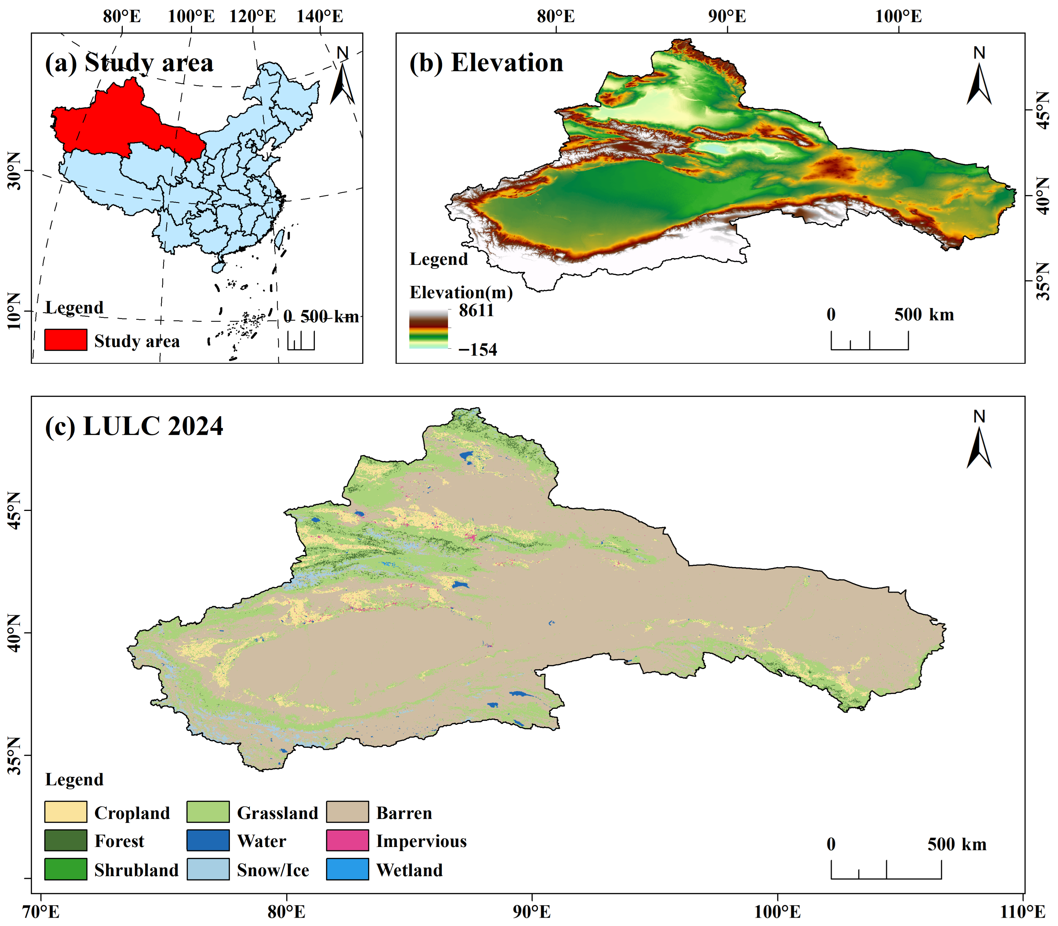
The ARNC (35°N–50°N, 73°E–106°E), located in the Eurasian hinterland, functions as a vital national ecological barrier and a central node within the Silk Road Economic Belt (Figure 1) [23]. Structurally, the region exemplifies the MBS, with alternating high-altitude mountain ranges such as the Altai, Tianshan, and Qilian, and interior basins and corridors including the Tarim, Junggar, and Hexi Corridor [24,25]. This distinctive topography produces marked vertical zonality and landscape gradients, ranging from “alpine water towers” to mid-elevation oases and desert matrices [26]. The climate is characterized by extreme aridity, with mean annual precipitation of approximately 160 mm and potential evapotranspiration between 800 and 3200 mm, resulting in a significant hydrological deficit [27,28]. Oases, which occupy less than 10% of the land area, support more than 90% of the population and account for about 95% of water resource consumption [29]. Consequently, the spatial concentration of anthropogenic pressures heightens the ARNC’s vulnerability to hydrological variability and intensified land use [30,31].

2.2. Data Acquisition and Preprocessing

The RSEI was developed on the Google Earth Engine (GEE) platform using annual median composites of MODIS products for the growing season (April to October) from 2000 to 2024. Permanent water bodies were masked with the JRC Global Surface Water dataset prior to principal component analysis to avoid moisture bias in the principal component loadings. The input datasets comprised NDVI from MOD13A1 v061, surface reflectance bands from MOD09A1 v061 for calculating Wetness and Dryness components, and Land Surface Temperature (LST) from MOD11A2 v061. To achieve spatial consistency, thermal data were resampled from 1 km to 500 m resolution using bilinear interpolation.
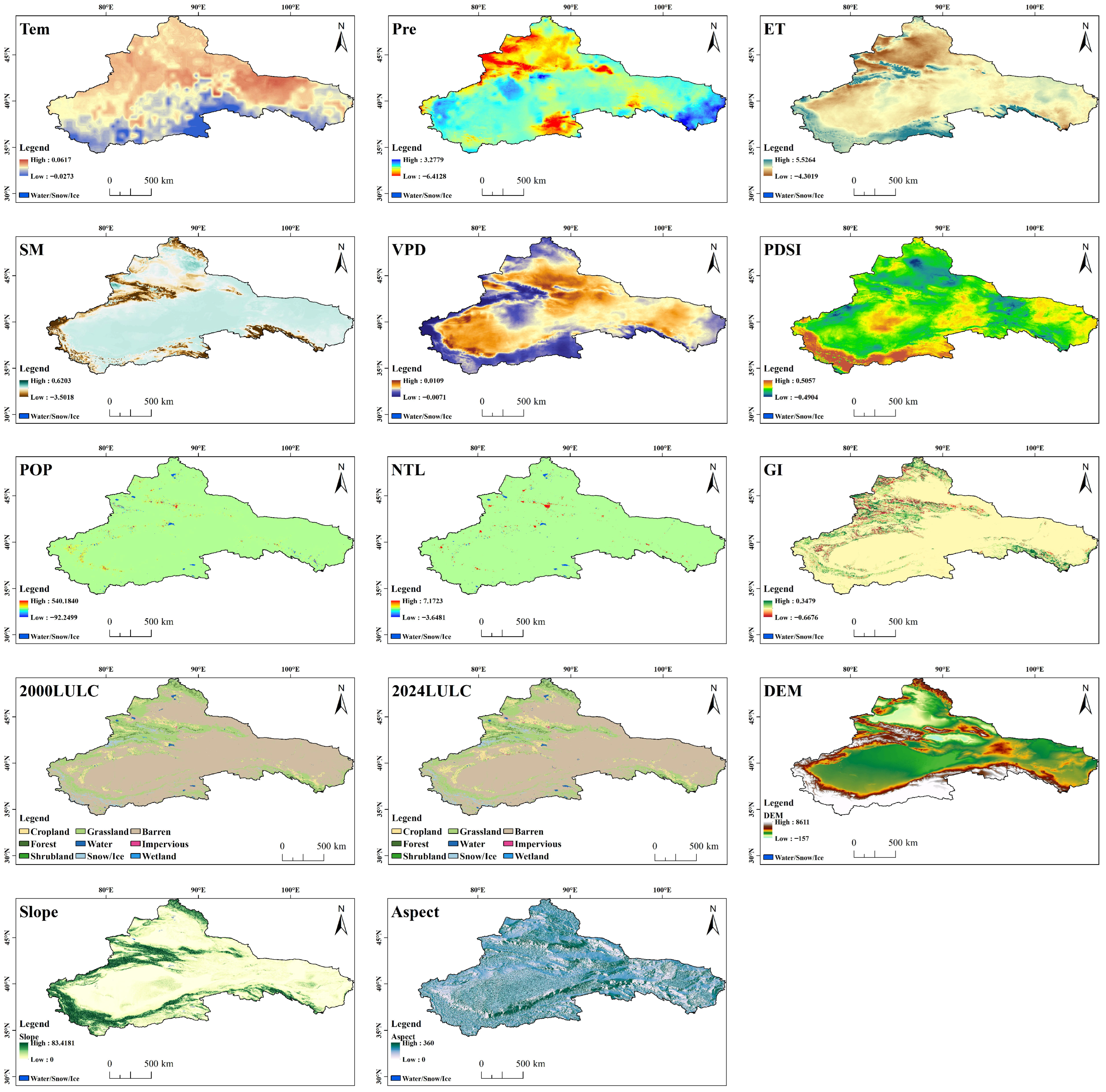
For attribution analysis, thirteen explanatory variables were compiled and categorized as either dynamic drivers or static controls (see Table 1 for details). Climatic variables, such as precipitation and temperature, were aggregated as annual means to represent long-term aridity trends influencing ecological evolution. All datasets were reprojected to the WGS 1984 coordinate system and standardized to a spatial resolution of 0.0045° (approximately 500 m). To maintain data fidelity, bilinear interpolation was applied to continuous variables to preserve spatial gradients, while the nearest neighbor method was used for categorical variables, such as land use and land cover (LULC), to maintain class integrity.

2.3. Methods

2.3.1. RSEI Construction

Based on the RSEI conceptual framework, EEQ was quantified by integrating four key dimensions: Greenness, Wetness, Heat, and Dryness.
(1) Greenness
Vegetation serves as a critical ecological barrier in arid regions. Greenness was represented by NDVI, which reflects vegetation growth status and coverage density [39].
(2) Heat
Heat was represented by LST derived from MOD11A2. LST characterizes the thermal stress and surface thermal emission intensity, acting as a critical limiting factor in arid ecosystems [40].
(3) Wetness
Wetness (WET), derived via the Tasseled Cap Transformation (TCT), captures moisture variations by modeling the spectral contrast between strong absorption in Shortwave Infrared (SWIR) bands and high reflectance in Visible-NIR bands [41]. The calculation based on MODIS surface reflectance is:
WET = 0.1147 ρ Red   +   0.2489 ρ N I R 1 + 0.2408 ρ Blue + 0.3132 ρ G r e e n 0.3122 ρ N I R 2 0.6416 ρ S W I R 1 0.5087 ρ S W I R 2
where ρRed through ρSWIR2 correspond to the surface reflectance values of MODIS Bands 1 through 7, respectively.
(4) Dryness
To capture surface aridity driven by both natural bare soil and anthropogenic impervious surfaces, the Normalized Difference Built-up and Soil Index (NDBSI) was employed, averaging the Soil Index (SI) and the Index-based Built-up Index (IBI) [42]. The calculation based on MODIS surface reflectance is:
SI   =   ( ρ S W I R 1 + ρ Red )     ( ρ Blue   ρ NIR ) ( ρ S W I R 1 + ρ Red ) + ( ρ Blue + ρ NIR )
IBI   = 2 ρ S W I R 1 ( ρ N I R 1 ρ N I R 1 + ρ Red + ρ Green ρ Green + ρ S W I R 1 ) 2 ρ S W I R 1 + ( ρ N I R 1 ρ N I R 1 + ρ Red + ρ Green ρ Green + ρ S W I R 1 )
NDBSI   = SI + IBI 2
where ρRed, ρNIR, ρBlue, ρGreen, and ρSWIR1 correspond to the surface reflectance values of MODIS Bands 1, 2, 3, 4, and 6, respectively.
To eliminate unit disparity, a Min-Max normalization standardized all indicators to a range of 0 to 1, calculated as follows:
N I i = I i I m i n I m a x I m i n
where NIi signifies the normalized value, while Ii corresponds to the original observation. Imax and Imin denote the upper and lower bounds of the indicator. This linear scaling procedure standardizes the dynamic range of all indicators, thereby removing potential biases caused by dimensional disparities. The four input indicators (NDVI, WET, LST, and NDBSI) inherently exhibit strong spectral and ecological correlations. For example, the cooling effect of vegetation results in a negative correlation between NDVI and LST. PCA leverages these correlations to transform redundant information into linearly uncorrelated orthogonal components. As a result, PC1 captures the coupled ecological signals by integrating the opposing effects of greenness and wetness versus heat and dryness, thereby enhancing the ecological interpretability of the final index.
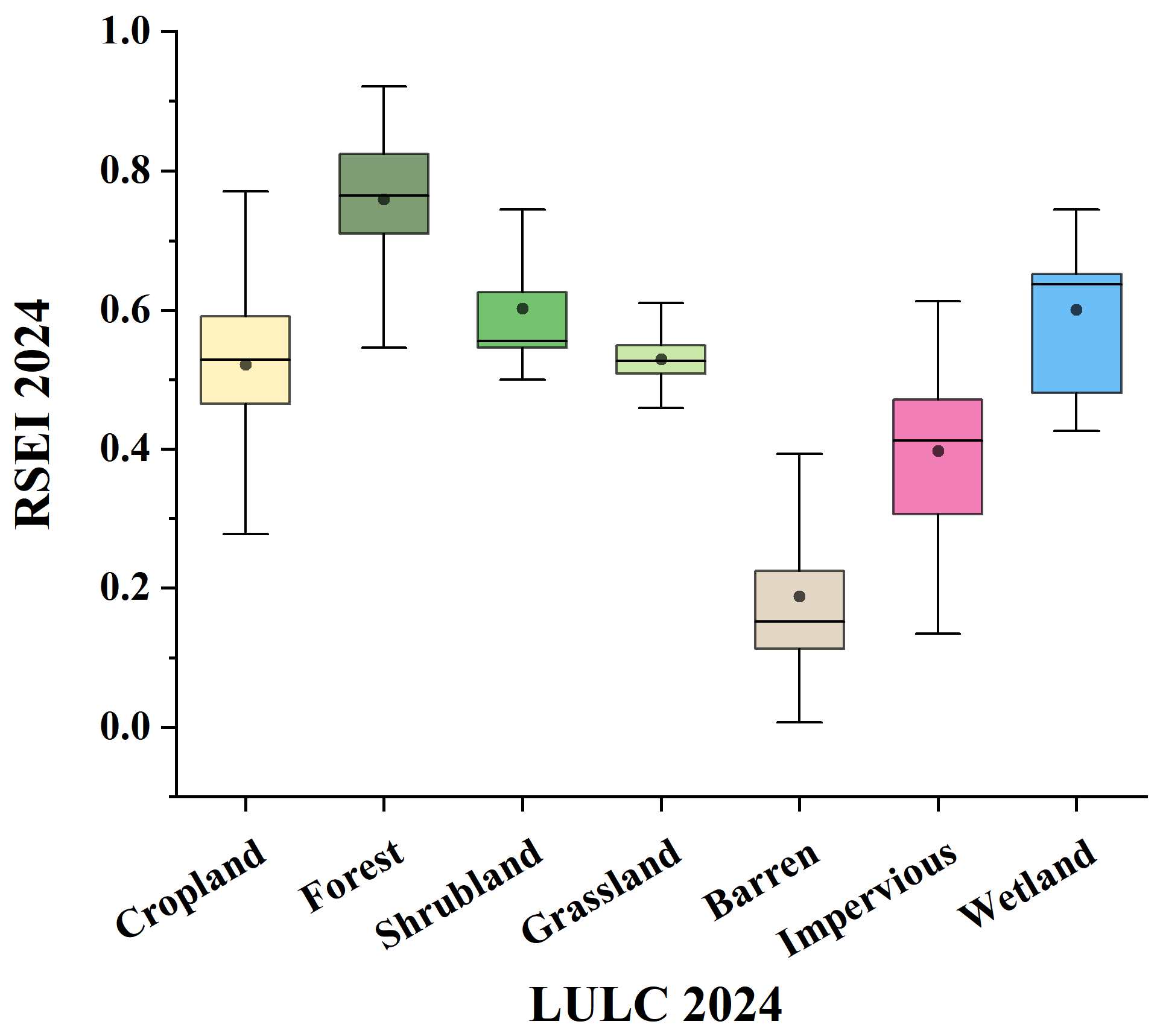
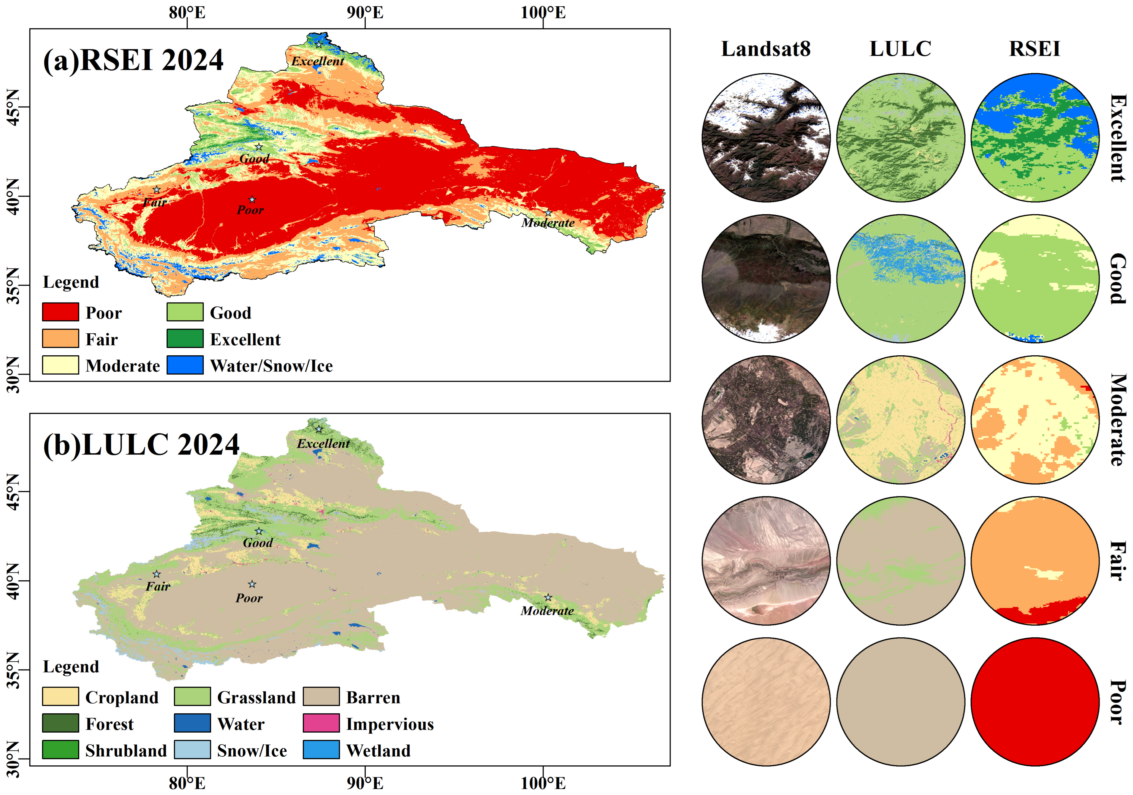
Statistical analysis of the component loadings (Table A2) supports the model’s validity and temporal robustness. During the study period (2000–2024), PC1 consistently explained the majority of the variance, with an average contribution of 71.33% ± 0.59%. LST displayed the most substantial negative loadings (−0.80 ± 0.03; range: −0.85 to −0.74), demonstrating that thermal stress is the principal driver of regional ecological differentiation. In contrast, NDBSI generally exhibited negative loadings (−0.02 ± 0.02) but contributed minimally to the variance, indicating a secondary role in this arid context. NDVI functioned as the primary positive regulator, with strong positive loadings (0.60 ± 0.04; range: 0.53–0.67), underscoring the importance of vegetation in mitigating thermal stress. Wet exhibited low magnitude and variable direction (mean: −0.01 ± 0.02). This pattern reflects a typical spectral response in hyper-arid environments, where the Tasseled Cap Wetness component is often influenced by the high reflectance of bright soil backgrounds and salt crusts, rather than by actual moisture content. Consequently, this weak negative loading should be interpreted as a region-specific signal feature, confirming that the regional RSEI is primarily governed by the heat-greenness regulatory mechanism. To further corroborate the index’s reliability in the absence of regional ground truth, an indirect validation was conducted. The RSEI demonstrated high logical consistency with LULC categories and exhibited strong spatial agreement with true-color reference imagery (Figure A1 and Figure A2), confirming its capacity to accurately reflect the regional ecological status.
Because PC1 is positively correlated with ecological benefits (Greenness) and negatively correlated with stressors (Heat and Dryness), the initial RSEI0 was defined directly as PC1. Thus, the inversion step, typically required when PC1 represents ecological degradation, was omitted:
R S E I 0 = P C 1
Subsequently, to facilitate spatiotemporal comparability, RSEI0 was normalized to a range of 0 to 1 to yield the final index:
R S E I = R S E I 0 R S E I 0   m i n R S E I 0   m a x R S E I 0   m i n
where RSEI0 denotes the initial ecological index derived from the first principal component; RSEI represents the final standardized index; and RSEI0 max and RSEI0 min correspond to the maximum and minimum values of the initial index, respectively.
Finally, drawing upon the classification framework of the Technical Criterion for Ecosystem Status Evaluation (HJ 192-2015) [18,40], the standardized RSEI was stratified into five distinct levels using the equal interval method: Poor (0–0.2), Fair (0.2–0.4), Moderate (0.4–0.6), Good (0.6–0.8), and Excellent (0.8–1.0). This grading system provides a standardized basis for quantifying regional ecological dynamics.

2.3.2. Spatiotemporal Trend Analysis

To quantify the long-term spatiotemporal trajectories of EEQ and its driving forces from 2000 to 2024, this study employed the Theil-Sen slope estimator for all continuous variables, coupled with the Mann–Kendall (MK) significance test specifically for the RSEI. This non-parametric approach is widely favored in ecological and hydrological time-series analysis due to its robustness against data outliers and insensitivity to distributional assumptions [43].
(1) Theil-Sen Slope Estimator
The Theil-Sen estimator calculates the median slope of all possible data pairs to represent the magnitude of the trends. Compared to traditional ordinary least squares regression, this method effectively mitigates the interference of noise inherent in long-term remote sensing datasets. The calculation is defined as:
β = median X j     X i j     i ,   2000 i < j 2024
where X denotes the specific time-series variable (including RSEI and continuous dynamic driving factors) and β represents the trend slope. A value of β > 0 denotes a numerically increasing trend (corresponding to ecological improvement specifically in the context of RSEI), while β < 0 signifies a decreasing trend.
(2) Mann–Kendall Significance Test
To determine the statistical validity of the ecological trajectories, the Mann–Kendall test was applied exclusively to the RSEI time series. This method assesses monotonic trends without requiring the data to follow a specific distribution. The test statistic S is calculated as:
S = i = 1 n 1 j = i + 1 n sgn ( R S E I j R S E I i )
sgn θ =     1    ,   ( θ > 0 )     0    ,   ( θ = 0 ) 1    ,   ( θ < 0 )
where RSEIi and RSEIj denote the RSEI values at years i and j (j > i), respectively; n is the length of the time series; sgn is the sign function; and Var(S) represents the variance of the statistic S. For n > 10, the statistic S approximates a standard normal distribution. Assuming no tied values in the time series, the standardized test statistic Z is computed as follows:
Z   = S 1 var ( S )    ,   ( S > 0 )         0           ,   ( S = 0 ) S + 1 var ( S )    ,   ( S < 0 )
var ( S ) = n ( n 1 ) ( 2 n 5 ) 18
In this study, a confidence level of 95% was adopted (|Z| > 1.96) to identify significant trends in EEQ.
Based on the computed slope (β) and significance (Z) derived from the entire 25-year time series (2000–2024), the spatiotemporal patterns of RSEI were categorized into three distinct classes to interpret long-term ecological evolution. The specific classification criteria are detailed in Table 2.

2.3.3. Stability Analysis

To assess the temporal stability of EEQ in the ARNC, the Coefficient of Variation (CV) was employed. As a standardized metric of dispersion, the CV effectively quantifies the magnitude of interannual fluctuations relative to the long-term mean. The calculation is formulated as:
CV = σ x ¯
where CV denotes the coefficient of variation; σ represents the standard deviation of the RSEI time series for each individual pixel; and x ¯ corresponds to the multi-year mean RSEI value. A higher CV value indicates greater volatility and lower stability of the ecosystem. ‘Stability’ in this context refers specifically to the low magnitude of interannual statistical fluctuation, or temporal invariance. This definition does not encompass ‘ecological resilience’ (the capacity to recover from disturbance) or ‘ecosystem health.’ High stability values may reflect either a sustained high-quality state, such as stable forests, or a persistent low-value state, such as natural deserts limited by aridity.
Drawing upon classification schemes from comparable studies [44], the stability of EEQ was stratified into five distinct levels: High Stability (CV ≤ 0.10), Medium-High Stability (0.10 < CV ≤ 0.15), Medium Stability (0.15 < CV ≤ 0.20), Low Stability (0.20 < CV ≤ 0.30), and Extremely Low Stability (CV > 0.30).

2.3.4. Spatial Autocorrelation Analysis

Following the spatiotemporal trend analysis, the Local Moran’s I index was employed to reveal the spatial agglomeration patterns of ecological dynamics, using the RSEI trend slope (β) as the target variable [45]. Unlike global statistics that summarize regional averages, Local Moran’s I effectively identifies localized spatial clusters and significant outliers at the pixel level. The calculation is defined as:
I i = x i x ¯ S 2 j = 1 ,   j i N w i j ( x j x ¯ )
where Ii denotes the Local Moran’s I for the i-th pixel; xi and xj represent the trend slope (β) at locations i and j; x ¯ corresponds to the mean slope of the study area; S2 is the variance; N is the total number of pixels; and wij signifies the spatial weight matrix defined by Queen contiguity.
The statistical significance of Ii was assessed using a standard Z-score test. Only pixels passing the significance threshold (p < 0.05) were classified. The spatial patterns were stratified into four distinct association modes: High-High (H-H): High values surrounded by high values (Clusters of Improvement); Low-Low (L-L): Low values surrounded by low values (Clusters of Degradation); High-Low (H-L) and Low-High (L-H): Outliers indicating spatial heterogeneity.

2.3.5. Driver Attribution Analysis via XGBoost-SHAP Framework

To disentangle the complex, non-linear driving mechanisms underlying ecological dynamics, this study constructed an interpretable machine learning framework that couples the XGBoost model [46] with SHAP [47].
First, the XGBoost regression model was employed to predict the RSEI trend slope (β) using the 13 explanatory variables (Table 1) as inputs. Within this framework, input variables fulfill specific mechanistic functions. Dynamic variables, including climatic trends and anthropogenic activities, act as direct drivers that induce temporal changes in EEQ. In contrast, static variables such as DEM, Slope, and Aspect serve as background constraints or spatial modulators. Although static factors remain unchanged over time, they define the biophysical context, such as hydrothermal niches, which influence both the sensitivity and direction of ecosystem responses to dynamic drivers. Incorporating these variables enables the model to represent spatially heterogeneous non-linear interactions, as demonstrated by the varying effects of warming across elevation gradients. Unlike conventional linear regression approaches (e.g., OLS), the tree-based ensemble architecture of XGBoost effectively captures high-dimensional interactions and threshold effects inherent in arid ecosystems. To ensure model robustness and prevent overfitting, key hyperparameters (including the number of estimators, learning rate, and maximum depth) were optimized via a 10-fold cross-validation grid search. Furthermore, the model’s predictive performance was rigorously assessed using the Coefficient of Determination (R2) and Root Mean Square Error (RMSE) to guarantee its reliability for subsequent attribution.
Subsequently, to resolve the “black-box” opacity of the machine learning model, the SHAP method based on cooperative game theory was integrated. This framework decomposes the model’s prediction into the marginal contributions of each driver, ensuring consistent, locally accurate attribution. The calculation is defined as:
ϕ i = S F \ i S ! F S 1 ! F !   f S i x S i f S x S
where ϕ i denotes the SHAP contribution value for feature i; F represents the complete set of all features; S denotes a subset of features excluding i; and f S   ( x S ) is the model prediction using the feature subset S. This coupled framework facilitates a dual-level assessment of driving forces: (1) Global Importance Ranking, quantified by the mean absolute SHAP values to distinguish the dominance of natural versus anthropogenic factors; and (2) Non-linear Response Analysis, visualized via SHAP Dependence Plots to identify critical ecological thresholds and inflection points (e.g., the carrying capacity limit for grazing intensity).

3. Results

3.1. Temporal Characteristics and Landscape Structure

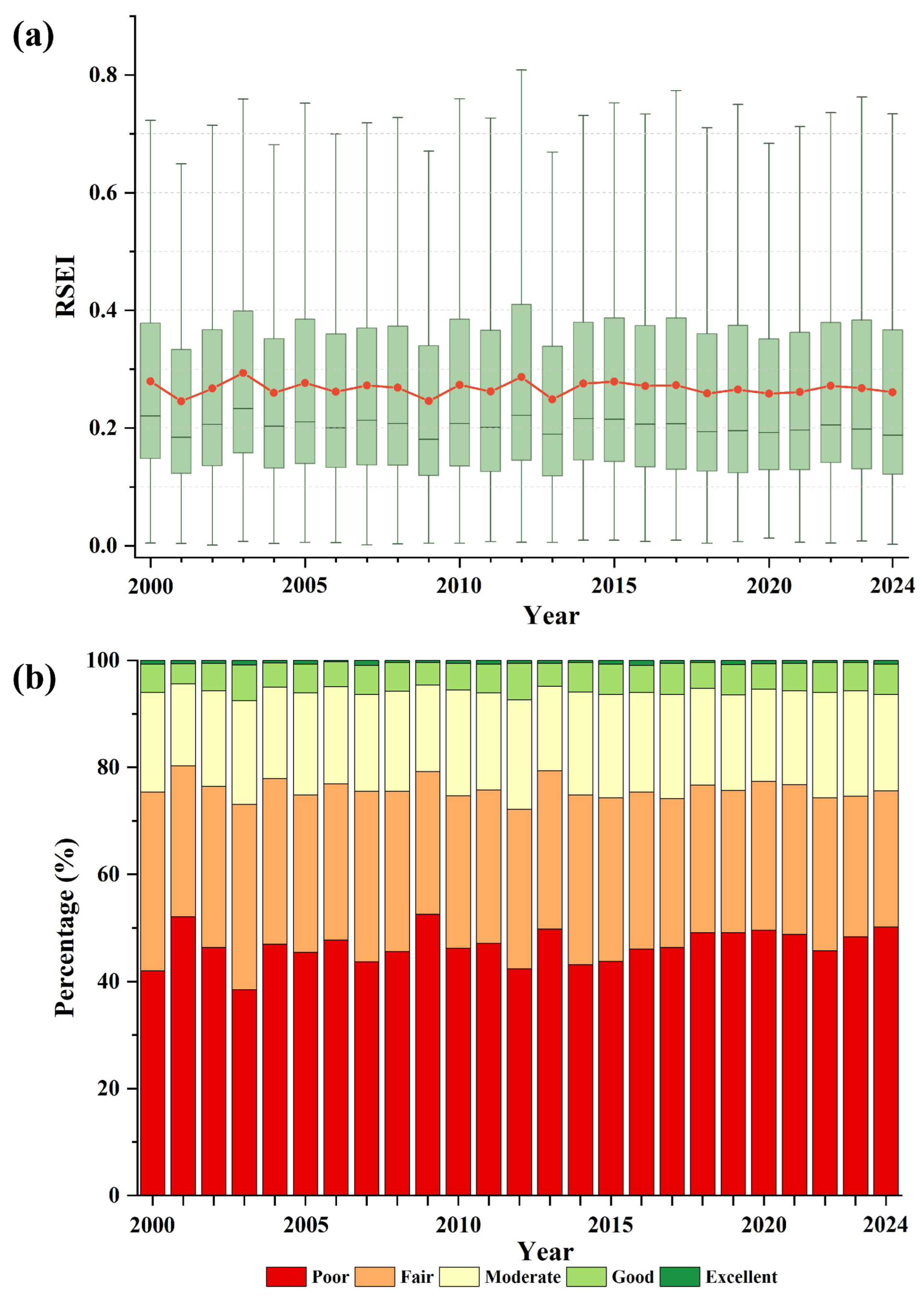
Between 2000 and 2024, the EEQ of the ARNC demonstrated stable, low-level fluctuations characteristic of water-limited ecosystems. Figure 2a shows that the annual mean RSEI remained within a narrow range of 0.25–0.30, with no statistically significant monotonic trend at the regional scale. The frequency distribution is strongly positively skewed, with a median near 0.20, indicating a predominance of low-value pixels in the regional matrix. Figure 2b supports this observation, showing that the ‘Poor’ and ‘Fair’ categories consistently accounted for over 70% of the total area. The persistence of this low-quality matrix suggests that the regional RSEI is fundamentally limited by the region’s inherent aridity.

3.2. Spatial Patterns and Ecosystem Stability

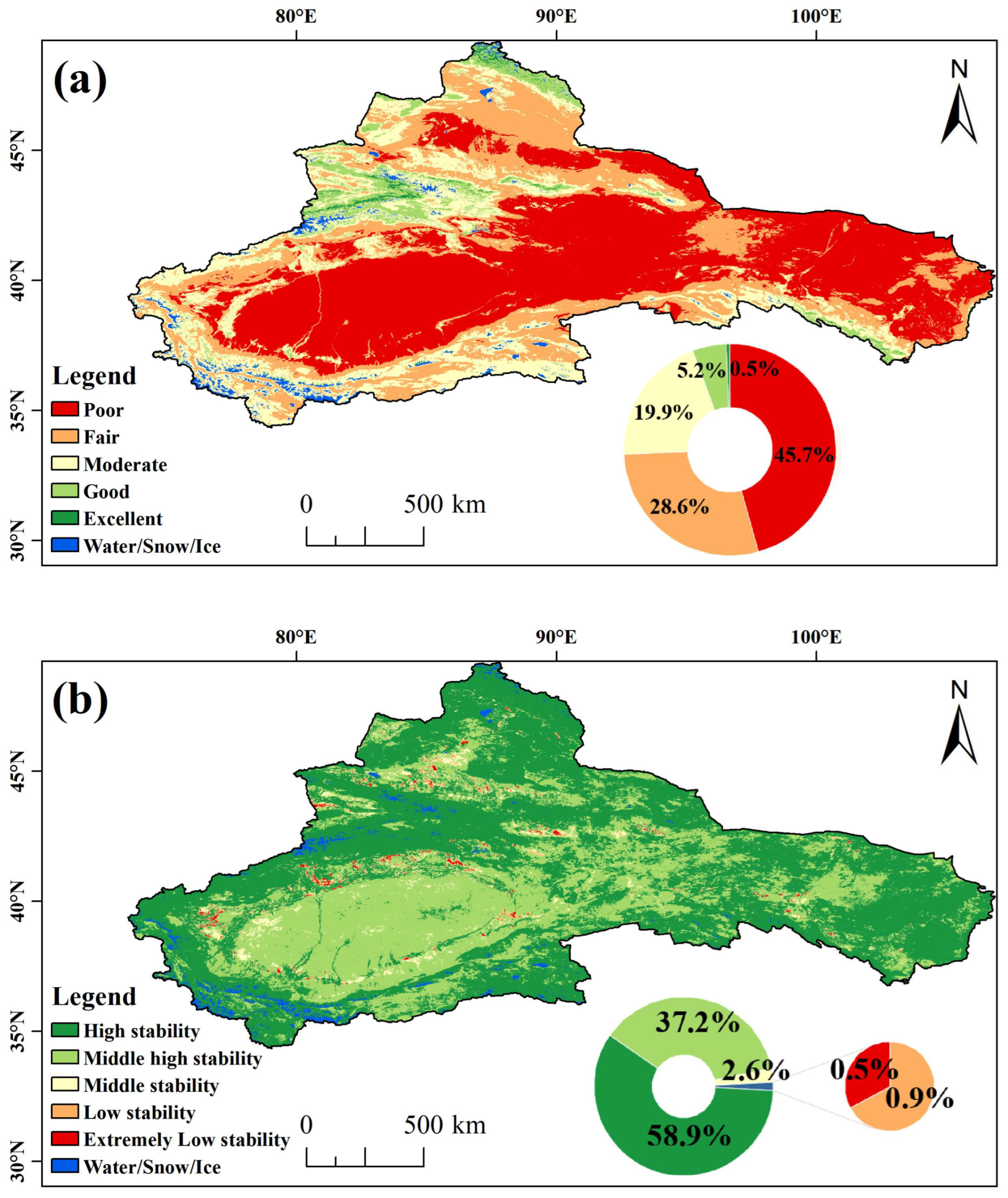
The multi-year mean RSEI displays pronounced spatial heterogeneity that closely follows geomorphological gradients, forming a distinct High-Mountain, Low-Basin pattern as depicted in Figure 3a. The ‘Good’ and ‘Excellent’ categories are restricted to high-altitude areas such as the Tianshan, Altai, and Qilian Mountains, while the ‘Poor’ category predominates in the interior basins and the Alxa Plateau. Ecosystem stability analysis (Figure 3b) indicates that 96.1% of the study area exhibits High or Medium-High stability. Spatial overlay analysis demonstrates that this stability is primarily associated with the extensive low-value ecological matrix. These stable zones predominantly correspond to the ‘Poor’ and ‘Fair’ RSEI categories, suggesting a form of static stability governed by biophysical constraints rather than by active ecological resilience. The expansive desert matrix thus remains structurally invariant due to resource limitations, in contrast to the dynamic stability observed in healthy vegetation systems. In contrast, areas with Low Stability are concentrated at oasis-desert ecotones, highlighting their function as dynamic hotspots influenced by hydrological variability and anthropogenic disturbance.

3.3. Spatiotemporal Trends and Spatial Clustering

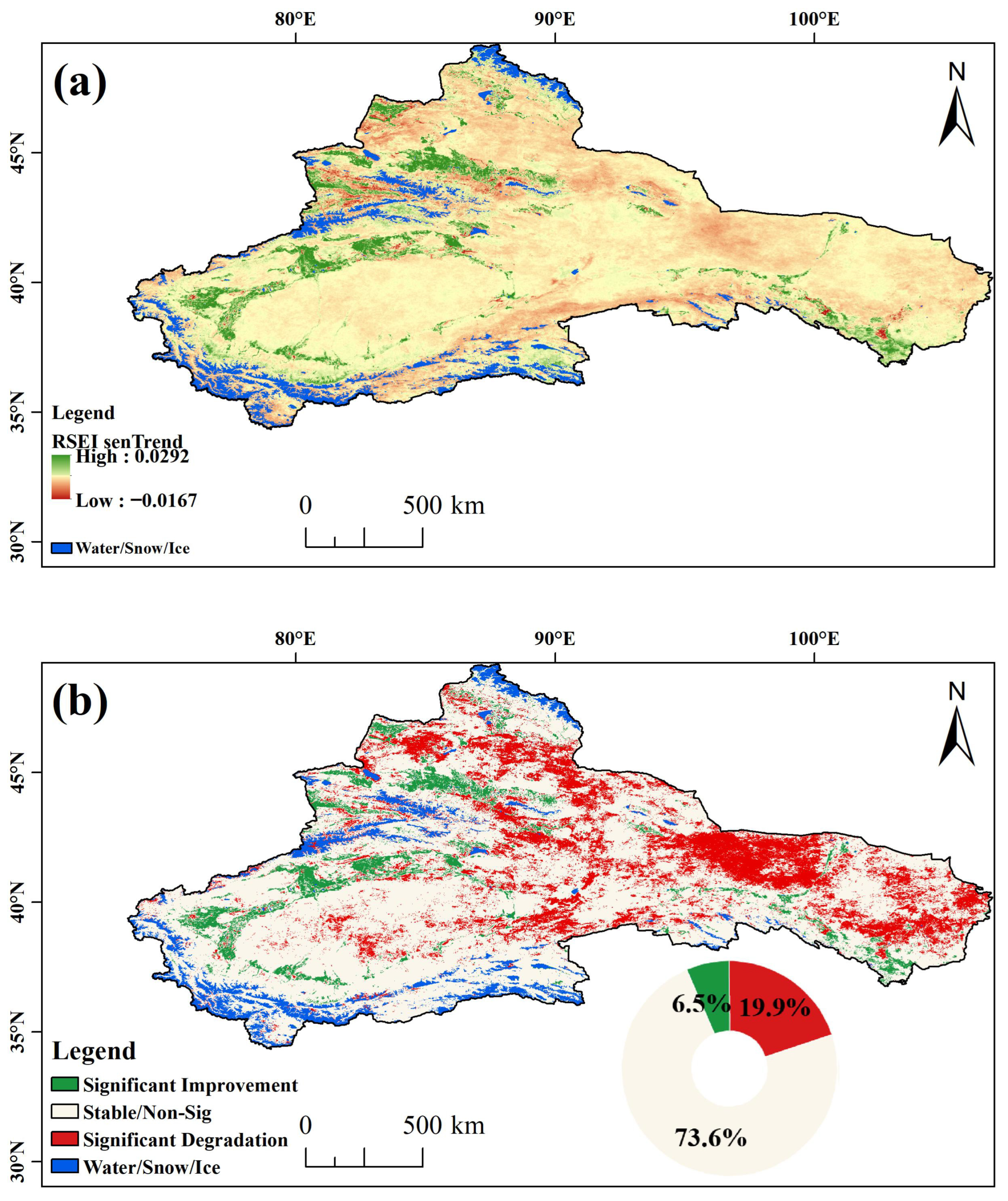
Pixel-wise Theil-Sen trend analysis, combined with the Mann–Kendall significance test (Figure 4) and Local Indicators of Spatial Association (Figure 5), was used to quantify spatiotemporal trajectories and spatial dependence of EEQ dynamics. Figure 4b shows that 73.6% of the region maintained a stable trajectory with non-significant trends, supporting the presence of ecological inertia driven by arid conditions. In areas with significant changes (p < 0.05), a pronounced asymmetry is observed: significant degradation (19.9%) affects more than twice the area of significant improvement (6.5%). Improvements are mainly concentrated in high-altitude mountain systems and the centers of artificial oases, while significant degradation is widespread across the eastern Alxa Plateau and the transitional zones surrounding the Tarim and Junggar Basins.
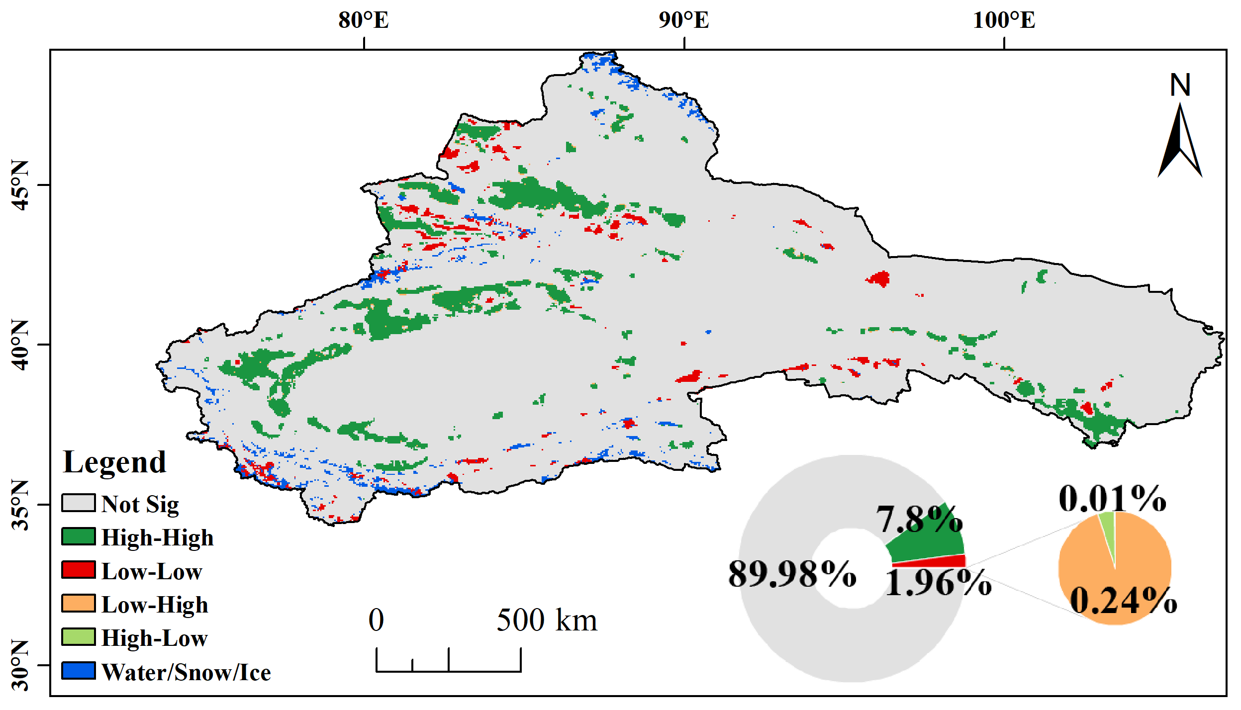
The LISA cluster map (Figure 5) provides additional insight into the spatial structure of these changes. Most of the study area (89.98%) exhibited non-significant spatial aggregation, suggesting that the extensive desert matrix does not display strong local dependence in its change patterns. Significant clustering was mainly observed as High-High clusters (7.8%), which align with improvement zones in mountainous and oasis areas, forming cohesive patches. In contrast, Low-Low clusters (1.96%) were scattered and fragmented. This comparison indicates that ecological improvement in the ARNC is a concentrated, localized phenomenon driven by targeted water availability, whereas degradation is a diffuse, widespread process likely resulting from large-scale climatic aridification.

3.4. Mechanisms of Ecological Improvement

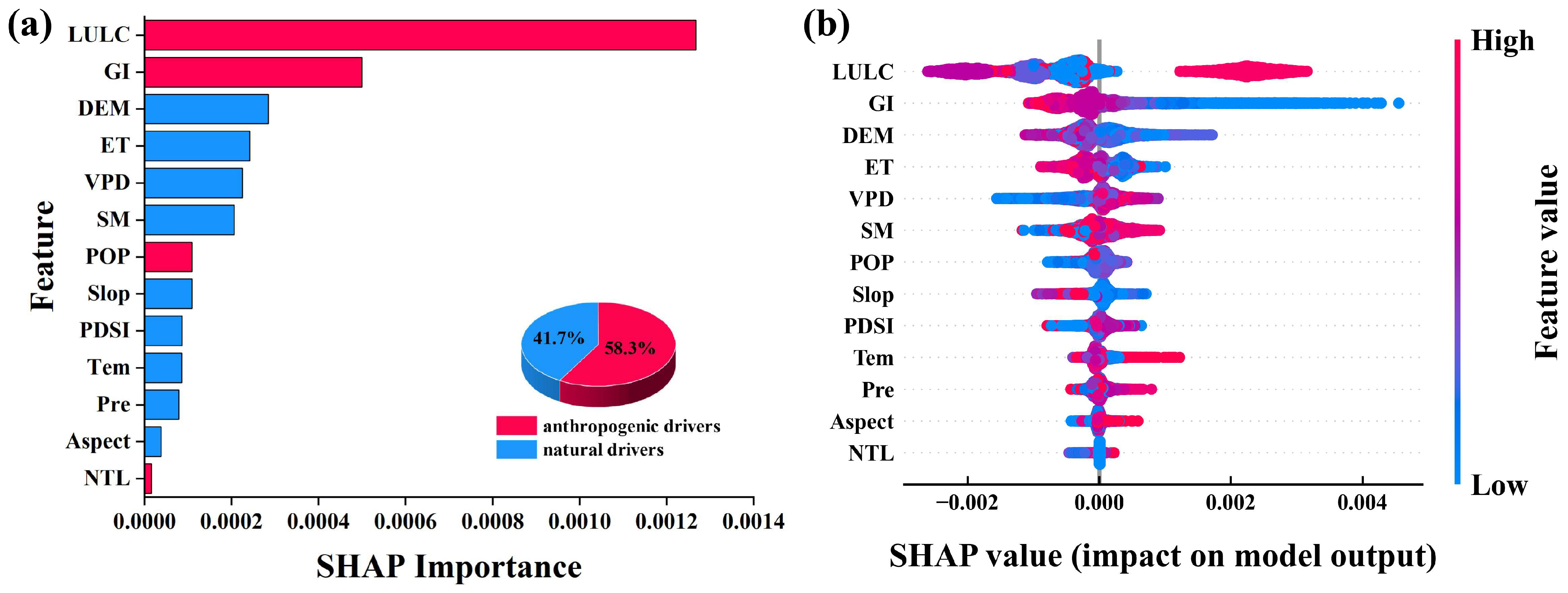
Analysis using the XGBoost-SHAP framework (R2 = 0.559) indicates that ecological improvement in the ARNC is primarily driven by anthropogenic factors, with natural regulation playing a supplementary role (Figure 6a). Anthropogenic drivers accounted for 58.3% of total feature importance, exceeding the 41.7% attributed to natural drivers. Among the predictors, LULC was the most influential, followed by GI and DEM. This hierarchy suggests that large-scale ecological recovery in the ARNC is predominantly the result of deliberate human intervention rather than passive natural processes.
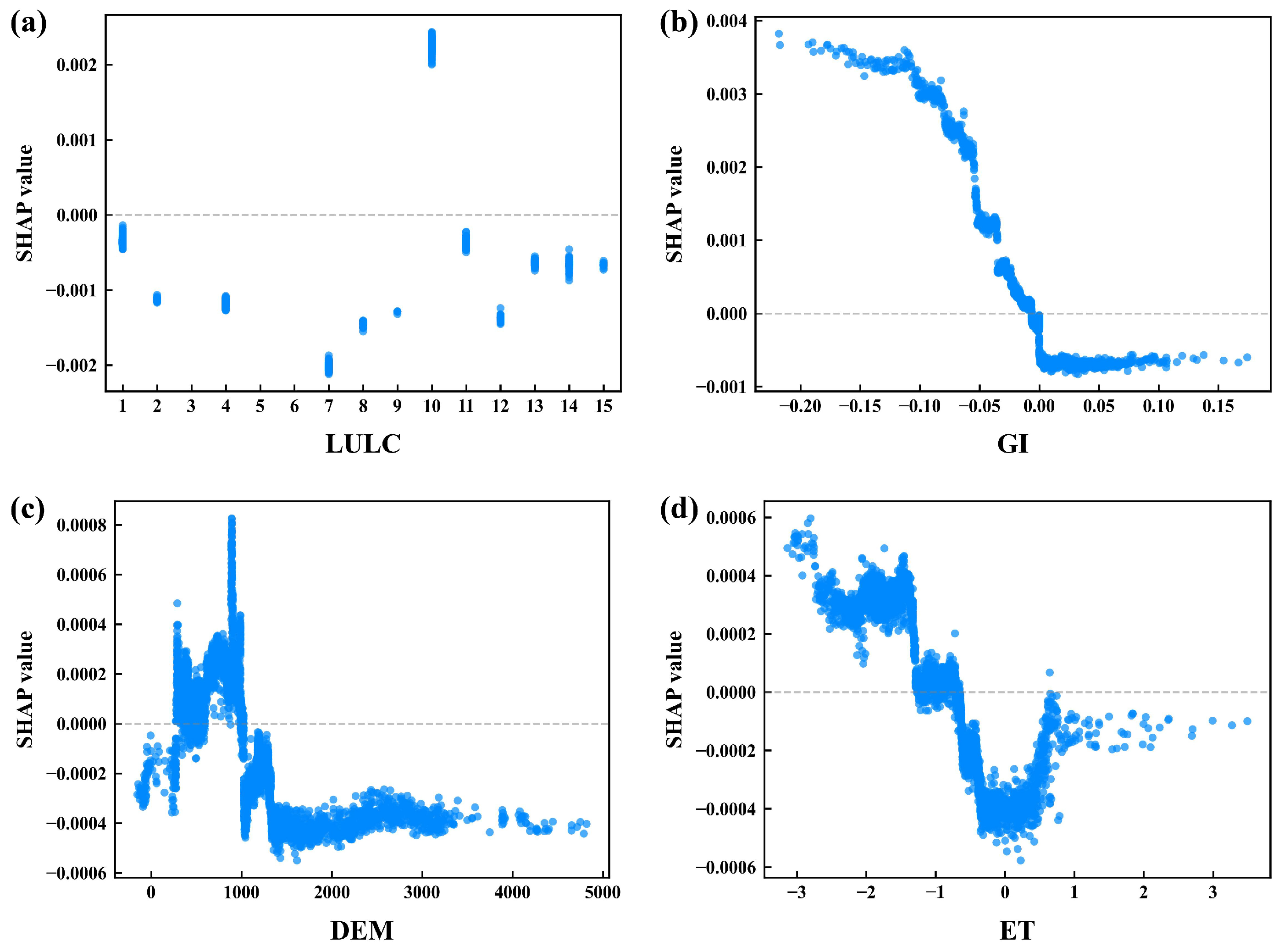
The SHAP dependence plots (Figure 7) illustrate the nonlinear marginal effects of key drivers. For LULC, the contributions are distinctly separated: Oasis Expansion (Code 10) produces the highest positive SHAP values (>0.002), whereas Stable Barren (Code 7) results in the most negative values (<−0.002). GI demonstrates a clear threshold effect, with positive SHAP values occurring only within negative GI ranges, corresponding to grazing alleviation. Conversely, positive GI values (>0) lead to an immediate decrease in SHAP values, which stabilize at a negative level of approximately −0.0008. The DEM reveals a unimodal pattern, with positive contributions restricted to the 300–1000 m elevation range and peaking near 900 m. ET exhibits a multi-stage response: SHAP values are positive when ET < −1, decline sharply to a minimum (SHAP ≈ −0.0005) within the –0.5 to 0.5 range, and, at higher ET values (>0.5), show a slight recovery but remain at a negative level (≈−0.0002), indicating a persistent negative contribution.

3.5. Mechanisms Driving Ecological Degradation

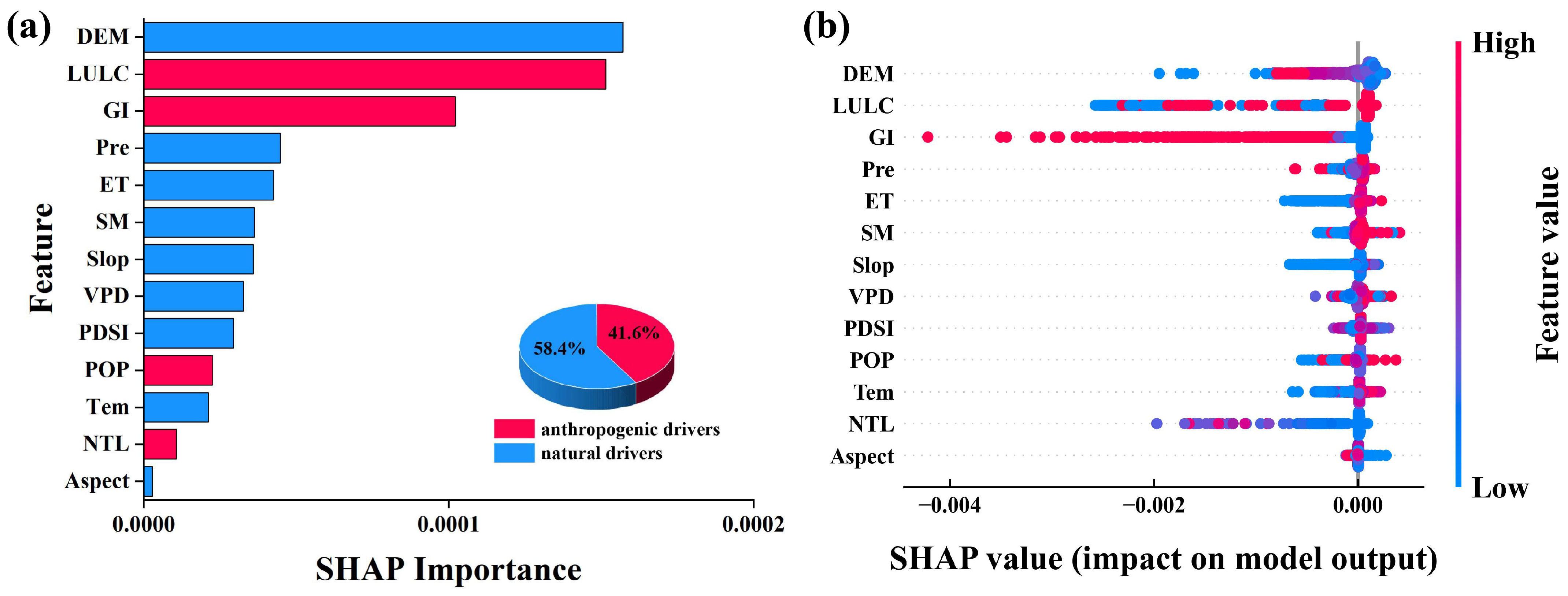
Unlike improvement zones, ecological degradation (R2 = 0.692) is primarily controlled by natural constraints, which are further intensified by anthropogenic stress (Figure 8a). Natural drivers account for 58.4% of the degradation mechanism, with DEM identified as the most influential factor. The higher predictive accuracy indicates that degradation processes in arid regions are more deterministic compared to improvement mechanisms.
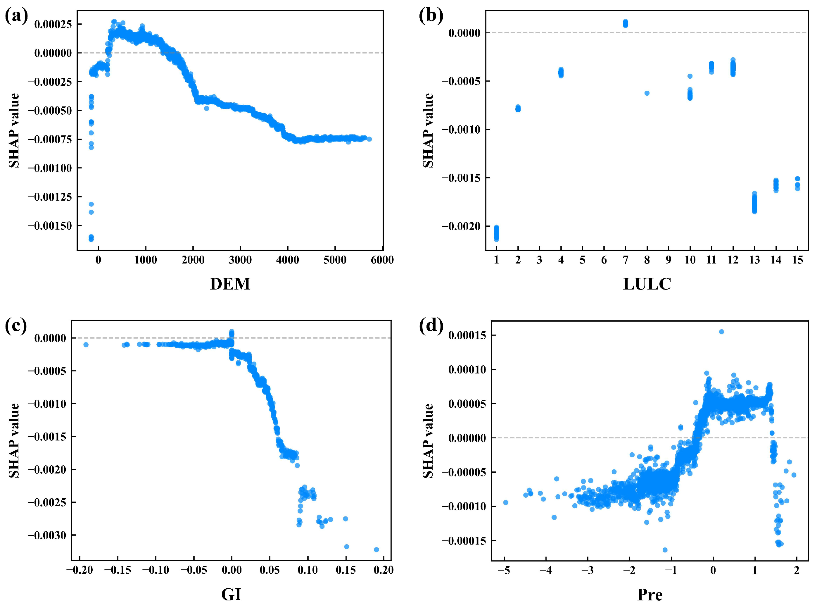
The SHAP dependence plots (Figure 9) reveal distinct nonlinear relationships among the analyzed variables. For DEM (Figure 9a), positive contributions are limited to the 200–1600 m elevation range, peaking near 350 m. Elevations above 1600 m show a monotonic decline, reaching a negative plateau of approximately −0.00075 above 4000 m. For LULC (Figure 9b), a clear hierarchy of negative impacts is evident among anthropogenic drivers: Stable Cropland (Code 1) imposes the greatest constraint (approximately −0.0021), followed by Cropland Abandonment (Code 13) at −0.0018, and Urbanization (Code 14) with a comparatively moderate negative effect (approximately −0.0016). This counterintuitive result, where long-term intensive cultivation negatively influences ecological quality, quantitatively supports the existence of a “Greenness-Quality Paradox” in the ARNC. GI (Figure 9c) demonstrates a critical asymmetric threshold. Ecological quality remains stable under grazing alleviation (GI < 0), but declines rapidly and in multiple stages with intensification (GI > 0). The response includes a sharp linear decline from GI 0.0 to 0.08, followed by an abrupt transition to a lower tier (approximately −0.0025 to −0.0032) at high intensity (GI > 0.10). This pattern suggests that pastoral overloading imposes the most severe, stepwise marginal pressure on ecosystem degradation. Pre (Figure 9d) exhibits a tri-phasic response: a stable negative baseline under drying conditions (Pre < −0.5, SHAP ≈ −0.00008), a rapid transition to a positive plateau under moderate wetting (0.0 < Pre < 1.4, SHAP ≈ +0.00005), and a sharp reversal at the extreme positive end (Pre > 1.5), where SHAP values decrease to approximately −0.00015.

4. Discussion

4.1. Spatial Asymmetry and Structural Constraints of Ecological Dynamics

Consistent with the regional MBS structure, the mean RSEI fluctuated narrowly between 0.25 and 0.30 (Section 3.1). This sustained low-level statistical stability aligns with broader assessments across Xinjiang and the Three-North Region, which consistently report that EEQ in these hyper-arid zones is statistically confined to low-value levels due to the dominance of the non-vegetated matrix [16,19,48]. Furthermore, this stability aligns with global dryland patterns, in which the upper limit of EEQ is tightly controlled by precipitation gradients, leading to a persistent low-cover state constrained by biophysical limits [49].
However, spatial clustering analysis (LISA) reveals a critical spatial asymmetry that complicates the notion of stability. Ecological improvements are concentrated in localized islands (High-High clusters, 7.8%), whereas degradation functions as a diffuse background process (19.9% trend compared to 1.96% clustering). This asymmetry reflects the distinct nature of these landscapes: the vast desert matrix maintains a structurally invariant state governed by aridity, whereas the improvement zones are fragile artificial systems that rely heavily on continuous human maintenance (e.g., irrigation) to prevent retrogression.
This apparent statistical stability may obscure the risk of a structural substitution. In the Junggar Basin, for example, improvements in RSEI are often driven by replacing natural desert ecosystems with artificial oases [13]. Although this conversion increases regional mean RSEI values due to higher greenness, it fragments the natural landscape and alters the surface energy balance [50]. Thus, the ‘Low-Level Stability’ of the ARNC likely represents a dynamic tension in which localized artificial greening attempts to counteract the structural inertia of the biophysically constrained natural matrix, rather than a static equilibrium of a healthy ecosystem.

4.2. Mechanistic Divergence and the “Greenness-Quality Paradox”

The analysis reveals a distinct mechanistic divergence: ecological improvement is predominantly driven by anthropogenic factors (58.3%), whereas degradation is structurally dominated by natural constraints (58.4%) but is also significantly exacerbated by anthropogenic influences (41.6%). These findings demonstrate that recovery in the ARNC is primarily influenced by anthropogenic inputs but remains strictly limited by biophysical constraints. The identification of DEM as the most significant factor for degradation (Figure 8a) highlights that elevation serves as a spatial determinant of ecological stability rather than a temporal driver. SHAP dependence plots (Figure 9a) reveal that topography delineates the landscape into two distinct ecological stability regimes. Fragile Highlands, situated above 1600 m, are characterized by negative SHAP values, reflecting inherent structural vulnerability where steep gradients amplify the impacts of pastoral overloading. Conversely, Stable Lowlands, spanning 200 to 1600 m, exhibit positive SHAP values, suggesting that flatter terrain provides a buffering effect that reduces degradation risks.
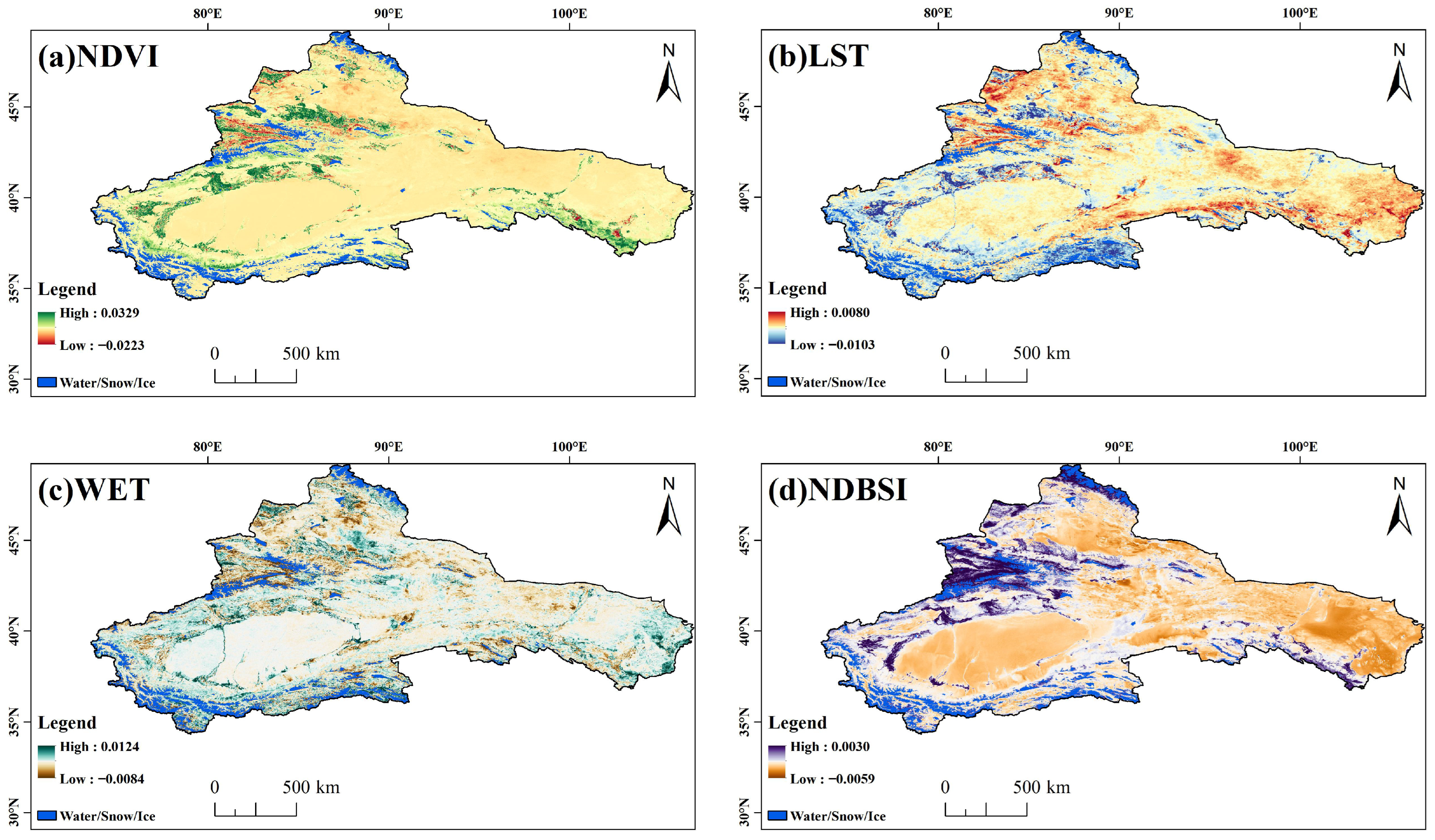
A comprehensive analysis of anthropogenic drivers reveals a “Greenness-Quality Paradox.” SHAP analysis quantifies this trade-off, demonstrating that long-term intensive cultivation (Stable Cropland, Code 1) imposes the most significant negative constraint on RSEI trends (SHAP ≈ −0.0021), exceeding the negative impact of Urbanization (SHAP ≈ −0.0016). This outcome challenges the prevailing assumption in arid basins that degradation is primarily due to impervious surface expansion [51,52], instead identifying high-water-consuming agriculture as the primary driver of ecological degradation. Divergent spatiotemporal patterns (Figure 10) corroborate this finding, as a substantial increase in Greenness (NDVI) coincides with stagnant Wetness (WET) and a notable rise in Dryness (NDBSI), rather than the anticipated improvement in moisture conditions.
The paradox arises from a “Water-for-Greenness” trade-off that disrupts the soil salt-water equilibrium. In stable oases, sustained irrigation elevates groundwater levels under high potential evapotranspiration, driving secondary salinization [14,53,54,55]. This physical deterioration—evidenced by the concurrent rise in NDBSI and NDVI—leads to diminished evaporative cooling, where the decline in soil health limits the reduction in LST despite increased vegetation cover. Since LST is a primary weighting factor in RSEI, this thermal inefficiency restricts overall ecological improvement. This mechanism supports the “masking effect” described by Zhao et al. [13] and aligns with the divergent trends observed in Northwest China, characterized by moderate increases in vegetation cover, contrasting with declines in overall EEQ [16,56], confirming that the region’s ecological quality is fundamentally constrained by substrate conditions (soil salinity and water-heat balance) rather than by vegetation cover alone. Ultimately, this soil degradation creates ecological liabilities, making Cropland Abandonment the second-most-severe anthropogenic driver of degradation (SHAP ≈ −0.0018).
In terms of spatial spillover, the high water demand of expanding oases functions as a siphon, intercepting groundwater recharge that previously sustained peripheral areas [57]. The implementation of high-efficiency water-saving technologies reduces lateral seepage, causing groundwater tables to fall below the survival threshold for native vegetation [58,59]. This hydrological mechanism explains the degradation pattern identified in Section 3.3, where deep-rooted shrubs in oasis-desert ecotones deteriorate due to anthropogenic hydrological cutoff [13,60]. Therefore, this hydrological siphon mechanism serves as a warning that artificial greening of oases may compromise the stability of surrounding natural transition zones.
The response to GI demonstrates a distinct zero-threshold effect (Figure 9c). The SHAP dependence plot indicates that ecological quality is preserved only when grazing alleviation occurs (GI < 0). In contrast, any increase in grazing intensity (GI > 0) triggers an immediate sharp linear decline, followed by a structural discontinuity at higher intensities (GI > 0.10). This deterministic pattern indicates that the ecosystem lacks resilience against pastoral overloading, with any intensification beyond the baseline exerting severe, stepwise marginal pressure on degradation.

4.3. Differentiated Management Strategies Under the RAD Framework

By integrating the identified spatial asymmetry and water-greenness trade-offs, a refined RAD strategy is proposed for distinct landscape zones [22]. For the “Direct” strategy in oasis cores, policy should shift from expansion to achieving salt-water balance regulation. In light of the negative impact of Stable Cropland, the assumption that increased vegetation necessarily equates to improved quality must be reassessed. Management should strictly limit agricultural water consumption to prevent the Jevons Paradox, in which efficiency gains inadvertently drive further expansion [61,62]. Priorities should focus on drainage improvements and salt management to decouple NDBSI increases from NDVI growth.
For grazing-sensitive zones such as ecotones and alpine pastures, a “Resist” strategy is essential. The identification of a critical sensitivity threshold near the equilibrium point (GI ≈ 0) underscores the vulnerability of these ecosystems. A minor transition from grazing alleviation to intensification may result in irreversible degradation of native vegetation, primarily due to the depletion of soil seed banks and changes in soil properties [63,64]. In this context, resistance requires protecting the existing natural interface. Strict enforcement of ecological water rights [65,66] is necessary to maintain groundwater levels above the critical survival depth for native shrubs [67,68], thereby preventing retreat of the oasis edge.
In the extensive desert matrix, an “Accept” strategy is the most scientifically viable approach. Since degradation in these areas is driven by broad-scale climatic factors such as precipitation and VPD thresholds [69,70], aggressive artificial revegetation, including high-density planting, contravenes the principle of water-based greenery and increases the risk of soil drying [71,72]. Therefore, the recommended strategy is to accept and monitor, minimizing human disturbance to preserve biological soil crusts [73,74]. This approach recognizes that a sparse, natural desert ecosystem is often more ecologically resilient than an artificial ecosystem subjected to high environmental stress.

4.4. Uncertainties and Future Perspectives

While RSEI effectively captures regional spatiotemporal patterns, specific limitations inherent to optical remote sensing in hyper-arid environments must be acknowledged. Primarily, there is an issue of optical insensitivity to sparse vegetation. In desert areas with less than 10% vegetation cover, the strong spectral reflectance of the bare soil background tends to suppress weak vegetation signals [75,76]. This “Mixed Pixel” effect may lead to the under-detection of early-stage degradation, potentially resulting in an overestimation of “stable” areas [77]. Furthermore, the index is constrained by subsurface invisibility and time lags [78]. As illustrated in Figure 10, RSEI captures surface Wetness but lacks the penetration depth to detect groundwater storage. The observed “Greenness-Quality Paradox” highlights a critical disconnection: surface greening often responds instantly to irrigation, while the depletion of deep groundwater is a cumulative, lagged process that optical indices cannot directly monitor [79].
To address these uncertainties, future research should prioritize multi-source data fusion, particularly by integrating downscaled gravity satellite data (e.g., GRACE/GRACE-FO) to explicitly account for groundwater storage anomalies. This integration bridges the scale gap between regional aquifer dynamics and local ecological indicators [78]. Additionally, advanced sensing technologies, such as hyperspectral and LiDAR sensors, should be used to distinguish specific soil salinity types and quantify the three-dimensional structure of sparse shrubs, thereby improving comprehensive monitoring of both vegetation structure and soil surface stability. Research should also expand into socio-hydrological modeling by incorporating Agent-Based Models, enabling simulation of farmer responses to proposed RAD strategies and explicit modeling of feedback loops between water rights enforcement and agricultural expansion.

5. Conclusions

This study elucidates the spatiotemporal dynamics and underlying mechanisms influencing EEQ in the ARNC. The principal conclusions are summarized as follows:
First, the ARNC demonstrates pronounced spatial asymmetry in ecological evolution, marked by low-level stability and significant dynamic imbalances. Ecological improvements are confined to localized, human-managed areas within oases, whereas degradation is widespread and diffuse, primarily driven by geomorphological inertia. These findings suggest that, while human intervention can establish isolated zones of high ecological quality, overcoming the broad biophysical constraints, especially topographic factors, in arid environments remains a significant challenge.
Second, the study quantitatively confirms the presence of a “Greenness-Quality Paradox” in arid agro-ecosystems. SHAP analysis reveals that long-term intensive cultivation decreases EEQ due to secondary salinization and diminished evaporative cooling, even when vegetation cover remains substantial. This result indicates that exclusive reliance on optical greenness indices may obscure significant risks associated with hydrological decoupling. Consequently, comprehensive evaluations of ecological restoration in drylands should integrate water-heat balance monitoring alongside surface vegetation metrics.
Third, effective management necessitates the identification of specific biophysical thresholds. The analysis indicates that ecological recovery is predominantly driven by human activities (58.3%), whereas degradation is mainly constrained by natural factors (58.4%). Importantly, a zero-threshold effect for grazing intensity was identified, whereby any increase above the baseline immediately diminishes ecological quality. In light of these findings, a Resist-Accept-Direct (RAD) framework is proposed: direct salt-water balance regulation in oases, resist hydrological cutoff in ecotones, and accept natural dynamics in the desert matrix. This differentiated approach offers a scientific foundation for reconciling human development with ecological resilience in water-limited regions.

Author Contributions

C.Y. Conceptualization, Methodology, Formal Analysis, Writing—original draft preparation. X.H.: Writing—Review and Editing, project administration, funding acquisition. Q.T.: Methodology, Visualization. J.L.: Methodology, Formal Analysis. Q.X.: Formal Analysis, Visualization. All authors have read and agreed to the published version of the manuscript.

Funding

This research was funded by the Xinjiang Uygur Autonomous Region Key Research and Development Project (No. 2024B03025-2), the Xinjiang Uygur Autonomous Region Key Research and Development Project (No. 2022B03030-2), and the Central Government Special Fund for Local Science and Technology Development (No. ZYYD2023A03).

Data Availability Statement

Publicly available datasets were analyzed in this study. The 1 km monthly temperature and precipitation datasets for China are available at the National Tibetan Plateau Data Center (Temperature: [https://doi.org/10.11888/Meteoro.tpdc.270961]; Precipitation: [https://doi.org/10.5281/zenodo.3114194]). The Extended NPP-VIIRS-like NTL data can be accessed via Harvard Dataverse [https://doi.org/10.7910/DVN/YGIVCD]. The China Land Cover Dataset (CLCD) is available on Zenodo [https://doi.org/10.5281/zenodo.15853565]. The 1980–2024 Grazing Intensity dataset (TED-LHGI) is accessible via the National Earth System Science Data Center and Figshare [https://doi.org/10.6084/m9.figshare.26195684.v3]. Other datasets were accessed via the Google Earth Engine (GEE) Data Catalog, including TerraClimate [https://developers.google.com/earth-engine/datasets/catalog/IDAHO_EPSCOR_TERRACLIMATE] (accessed on 9 November 2025), WorldPop [https://developers.google.com/earth-engine/datasets/catalog/WorldPop_GP_100m_pop] (accessed on 9 November 2025), and SRTM GL1 [https://developers.google.com/earth-engine/datasets/catalog/USGS_SRTMGL1_003] (accessed on 9 November 2025).

Conflicts of Interest

The authors declare no conflicts of interest.

Appendix A

Table A1. Classification system of LULC trajectories and their corresponding RSEI signal response mechanisms.
GroupCodeCategory NameEcological Definition and
Transition Logic
RSEI Signal Response Mechanism
Stable Stratum1Stable CroplandCropland → Cropland.
Represents the stable oasis matrix sustained by anthropogenic maintenance.
High Stable: Maintained by irrigation inputs (High WET, Low LST), though subject to salinization risks.
2Stable ForestForest → Forest.
Mountainous ecological barriers and riparian forests.
High Stable: High canopy density maintains high NDVI and regulates LST.
3Stable ShrublandShrubland → Shrubland.
Transition zone vegetation adapted to arid conditions.
Moderate Stable: Moderate NDVI; acts as a buffer against desertification.
4Stable GrasslandGrassland → Grassland.
Vast pastoral areas in alpine and basin fringe zones.
Moderate Stable: Seasonally variable NDVI; subject to grazing pressure.
5Stable WaterWater → Water.
Lakes, reservoirs, and permanent river channels.
Masked/High: Often masked in RSEI processing, but ecologically vital as a moisture source (Max WET).
6Stable Snow/IceSnow/Ice → Snow/Ice.
Alpine glaciers and permanent snow cover.
Masked/Low LST: Critical “Solid Reservoir” regulating regional hydrology.
7Stable BarrenBarren → Barren. The vast desert matrix (Gobi, sand dunes).Low Stable: Background state characterized by High LST, High NDBSI, and Low WET.
8Stable ImperviousImpervious → Impervious.
Established urban cores and industrial sites.
Low Stable: Dominated by the Urban Heat Island effect (High LST) and soil sealing (High NDBSI).
9Stable WetlandWetland → Wetland.
Natural swamps and marshes.
High Stable: High WET and biodiversity value.
Improvement10Oasis ExpansionNon-Cropland → Cropland (e.g., Barren → Cropland).
Anthropogenic land reclamation.
Strong Increase: Irrigation input leads to a sharp increase in WET/NDVI and a decrease in LST.
11Vegetation RecoveryBarren → Veg (Grassland/Shrubland/Forest). Ecological restoration or natural regrowth.Increase: Vegetation growth leads to NDVI increase and LST cooling effects.
Degradation12Vegetation DegradationVeg → Barren or Forest → Grassland. Loss of biomass due to stress or logging.Decrease: Loss of biomass leads to NDVI decrease and LST increase.
13Cropland AbandonmentCropland → Non-Cropland (Barren/Grassland). Cessation of farming and irrigation.Strong Decrease: Loss of artificial water inputs leads to sharp WET decline and LST rise (Retrogression).
14UrbanizationNatural/Cropland → Impervious. Urban sprawl and infrastructure construction.Decrease: Soil sealing leads to NDBSI increase and Heat Island intensification.
Others15OthersRare or illogical transitions (e.g., Impervio → Water).Mixed Signals: Irregular noise or classification errors.
Table A2. Annual statistics of PCA for RSEI construction (2000–2024), detailing the contribution rate, eigenvalues, and component loadings of the PC1.
YearNDVILSTWETNDBSIPC1 EigenvaluePC1 Contribution (%)
20000.5352−0.844−0.0337−0.00870.02373.18
20010.5897−0.8004−0.0187−0.1060.024371.56
20020.5964−0.8021−0.0292−0.00930.024771.29
20030.5339−0.8444−0.0353−0.02410.022272.37
20040.5733−0.81670.026−0.05990.022471.24
20050.5837−0.8108−0.0402−0.01410.025570.9
20060.5531−0.8325−0.0314−0.00030.023471.38
20070.593−0.8045−0.0325−0.00790.023371.14
20080.5347−0.8445−0.0292−0.00770.02370.6
20090.6042−0.796−0.037−0.00020.02471.14
20100.5788−0.81540.0113−0.00960.02570.98
20110.6034−0.79680.0237−0.02290.025971.56
20120.5307−0.8465−0.0405−0.00730.024370.44
20130.666−0.745−0.0391−0.02210.026371.89
20140.5435−0.83890.0199−0.02230.023171.39
20150.5792−0.8148−0.0233−0.00050.023971.77
20160.6476−0.76190.0055−0.00620.026371.45
20170.6157−0.7879−0.011−0.00350.027371.7
20180.6264−0.7794−0.0001−0.01010.024871.13
20190.664−0.7472−0.0211−0.01580.027871.67
20200.6482−0.761−0.0267−0.0010.025571.57
20210.6577−0.75270.0087−0.02980.026470.96
20220.5961−0.8028−0.0142−0.00260.024970.52
20230.5895−0.80740.0173−0.01880.02570.57
20240.6679−0.74430.00160.0020.02770.87
Mean ± SD0.5965 ± 0.0433−0.8000 ± 0.0324−0.0140 ± 0.0219−0.0163 ± 0.02240.0248 ± 0.001571.33 ± 0.59

Appendix B

Figure A1. Boxplots illustrating the distribution of RSEI 2024 values across distinct LULC 2024 categories. The gradient of RSEI values aligns with ecological logic, showing high values in ecological lands (Forest, Wetland) and significantly lower values in sparsely vegetated areas (Barren, Impervious), thereby confirming the ecological consistency of the index.
Remotesensing 18 00363 g0a1
Figure A2. Spatial validity check of the RSEI model. The comparison involves (a) the RSEI 2024 spatial distribution, (b) the LULC 2024 classification, and localized subsets comparing Landsat-8 OLI true-color composite imagery with LULC and RSEI classifications across five quality grades (Excellent to Poor).
Remotesensing 18 00363 g0a2
Figure A3. Spatiotemporal distribution patterns of potential driving factors for EEQ evolution in the ARNC (2000–2024).
Remotesensing 18 00363 g0a3
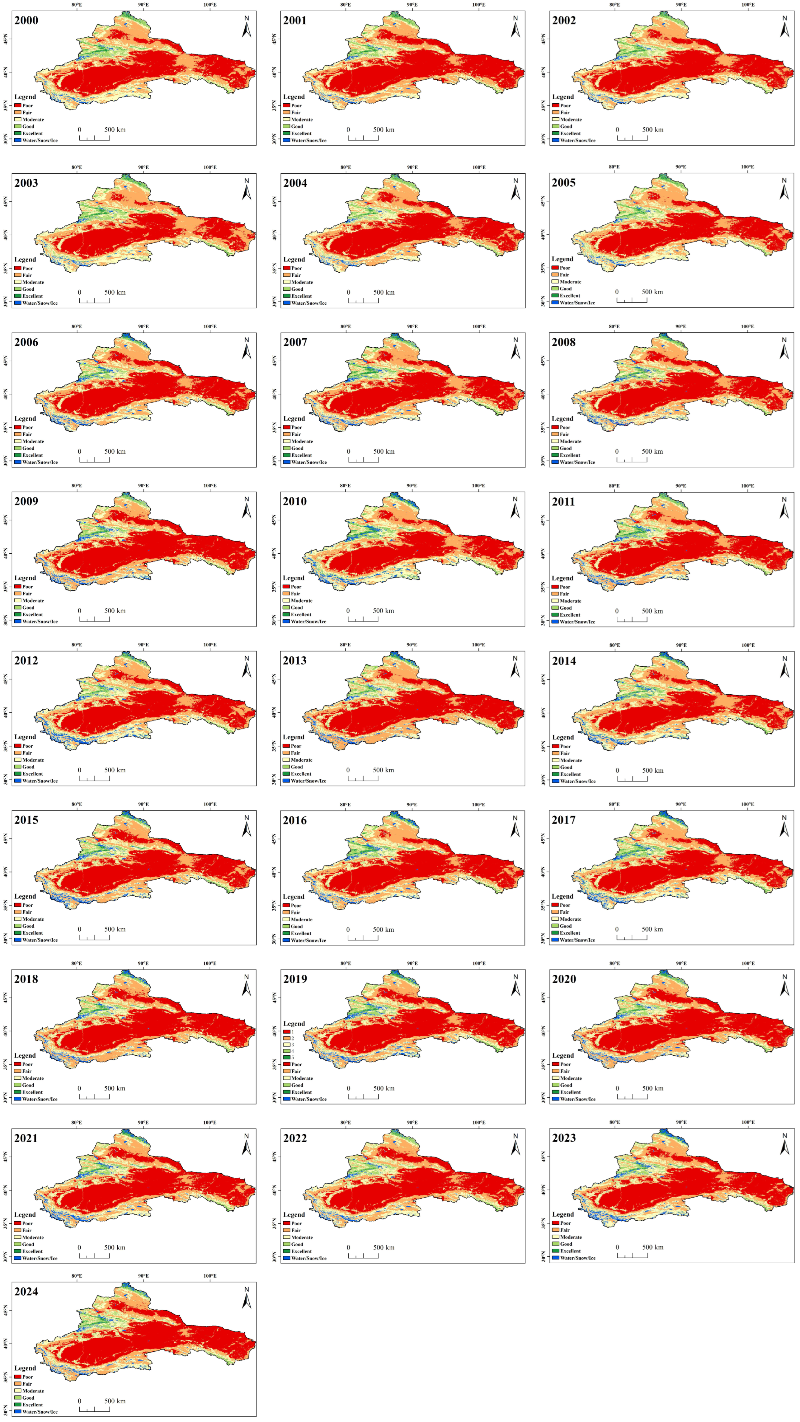
Figure A4. Spatiotemporal distribution patterns of EEQ in the ARNC (2000–2024).
Remotesensing 18 00363 g0a4

References

  1. Prăvălie, R. Drylands extent and environmental issues. A global approach. Earth-Sci. Rev. 2016, 161, 259–278. [Google Scholar] [CrossRef]
  2. Berdugo, M.; Delgado-Baquerizo, M.; Soliveres, S.; Hernández-Clemente, R.; Zhao, Y.; Gaitán, J.J.; Gross, N.; Saiz, H.; Maire, V.; Lehmann, A.; et al. Global ecosystem thresholds driven by aridity. Science 2020, 367, 787–790. [Google Scholar] [CrossRef]
  3. Huang, J.; Yu, H.; Guan, X.; Wang, G.; Guo, R. Accelerated dryland expansion under climate change. Nat. Clim. Change 2016, 6, 166–171. [Google Scholar] [CrossRef]
  4. Chen, Y.; Li, Z.; Fan, Y.; Wang, H.; Deng, H. Progress and prospects of climate change impacts on hydrology in the arid region of northwest China. Environ. Res. 2015, 139, 11–19. [Google Scholar] [CrossRef]
  5. Qi, Z.; Cui, C.; Jiang, Y.; Chen, Y.; Ju, J.; Guo, N. Changes in the spatial and temporal characteristics of China’s arid region in the background of ENSO. Sci. Rep. 2022, 12, 17826. [Google Scholar] [CrossRef] [PubMed]
  6. Chi, H.; Wu, Y.; Zheng, H.; Zhang, B.; Sun, Z.; Yan, J.; Ren, Y.; Guo, L. Spatial patterns of climate change and associated climate hazards in Northwest China. Sci. Rep. 2023, 13, 10418. [Google Scholar] [CrossRef] [PubMed]
  7. Lai, J.; Li, Y.; Chen, J.; Niu, G.-Y.; Lin, P.; Li, Q.; Wang, L.; Han, J.; Luo, Z.; Sun, Y. Massive crop expansion threatens agriculture and water sustainability in northwestern China. Environ. Res. Lett. 2022, 17, 034003. [Google Scholar] [CrossRef]
  8. Huang, Y.; Zhao, Y.; Gong, B.; Yang, J.; Li, Y. Effects of Potential Large-Scale Irrigation on Regional Precipitation in Northwest China. Remote Sens. 2024, 16, 58. [Google Scholar] [CrossRef]
  9. Sun, F.; Li, Y.; Chen, Y.; Fang, G.; Duan, W.; Li, B.; Li, Z.; Hao, X.; Yang, Y.; Zhang, X. The dominant warming season shifted from winter to spring in the arid region of Northwest China. npj Clim. Atmos. Sci. 2024, 7, 178. [Google Scholar] [CrossRef]
  10. Kerr, J.T.; Ostrovsky, M. From space to species: Ecological applications for remote sensing. Trends Ecol. Evol. 2003, 18, 299–305. [Google Scholar] [CrossRef]
  11. Leginio, M.D.; Agrillo, A.; Congedo, L.; Munafò, M.; Riitano, N.; Terribile, F.; Manna, P. Analysis of trends in productivity metrics in assessing land degradation: A case study in the Campania region of southern Italy. Ecol. Indic. 2024, 161, 111962. [Google Scholar] [CrossRef]
  12. Sui, X.; Xu, Q.; Tao, H.; Zhu, B.; Li, G.; Zhang, Z. Vegetation Dynamics and Recovery Potential in Arid and Semi-Arid Northwest China. Plants 2024, 13, 3412. [Google Scholar] [CrossRef]
  13. Zhao, N.; Du, L.; Tian, S.; Zhang, B.; Zheng, X.; Li, Y. Cropland Expansion Masks Ecological Degradation: The Unsustainable Greening of China’s Drylands. Agronomy 2025, 15, 1162. [Google Scholar] [CrossRef]
  14. Abliz, A.; Tiyip, T.; Ghulam, A.; Halik, Ü.; Ding, J.-l.; Sawut, M.; Zhang, F.; Nurmemet, I.; Abliz, A. Effects of shallow groundwater table and salinity on soil salt dynamics in the Keriya Oasis, Northwestern China. Environ. Earth Sci. 2016, 75, 260. [Google Scholar] [CrossRef]
  15. Xu, H. A remote sensing urban ecological index and its application. Acta Ecol. Sin. 2013, 33, 7853–7862. [Google Scholar]
  16. Zhang, L.; Li, X.; Liu, X.; Lian, Z.; Zhang, G.; Liu, Z.; An, S.; Ren, Y.; Li, Y.; Liu, S. Dynamic monitoring and drivers of ecological environmental quality in the Three-North region, China: Insights based on remote sensing ecological index. Ecol. Inform. 2025, 85, 102936. [Google Scholar] [CrossRef]
  17. Zhang, L.; Zhai, J.; He, F.; Li, X.; Wang, T. Dynamic monitoring of ecological security patterns in arid zone oases: A remote sensing-based ecological index evolution analysis. Sci. Rep. 2025, 16, 383. [Google Scholar] [CrossRef] [PubMed]
  18. Maimaitituersun, A.; Yang, H.; Aobuliaisan, N.; Maimaitiaili, K.; Chenyu, O. Assessing subtle changes in arid land river basin ecological quality: A study utilizing the PIE engine platform and RSEI. Ecol. Indic. 2025, 170, 113035. [Google Scholar] [CrossRef]
  19. Zhang, J.; Zhang, P.; Deng, X.; Ren, C.; Deng, M.; Wang, S.; Lai, X.; Long, A. Study on the Spatial and Temporal Trends of Ecological Environment Quality and Influencing Factors in Xinjiang Oasis. Remote Sens. 2024, 16, 1980. [Google Scholar] [CrossRef]
  20. Gong, C.; Lyu, F.; Wang, Y. Spatiotemporal change and drivers of ecosystem quality in the Loess Plateau based on RSEI: A case study of Shanxi, China. Ecol. Indic. 2023, 155, 111060. [Google Scholar] [CrossRef]
  21. Scheffer, M.; Carpenter, S.; Foley, J.A.; Folke, C.; Walker, B. Catastrophic shifts in ecosystems. Nature 2001, 413, 591–596. [Google Scholar] [CrossRef]
  22. Lynch, A.J.; Thompson, L.M.; Beever, E.A.; Cole, D.N.; Engman, A.C.; Hawkins Hoffman, C.; Jackson, S.T.; Krabbenhoft, T.J.; Lawrence, D.J.; Limpinsel, D.; et al. Managing for RADical ecosystem change: Applying the Resist-Accept-Direct (RAD) framework. Front. Ecol. Environ. 2021, 19, 461–469. [Google Scholar] [CrossRef]
  23. Zhang, J.; Yang, T.; Deng, M.; Huang, H.; Han, Y.; Xu, H. Spatiotemporal variations and its driving factors of NDVI in Northwest China during 2000–2021. Environ. Sci. Pollut. Res. 2023, 30, 118782–118800. [Google Scholar] [CrossRef]
  24. Yao, J.; Chen, Y.; Guan, X.; Zhao, Y.; Chen, J.; Mao, W. Recent climate and hydrological changes in a mountain–basin system in Xinjiang, China. Earth-Sci. Rev. 2022, 226, 103957. [Google Scholar] [CrossRef]
  25. Ma, R.; Zhang, Z.; Liu, L.; Zhang, M.; Ma, C.; Cao, Y.; Gao, Y.; Zhang, X.; Liu, X.; Zhang, J.; et al. Vegetation coverage patterns in the “mountain–basin” system of arid regions: Driving force contribution, non-stationarity, and threshold effects. Ecol. Inform. 2025, 87, 103084. [Google Scholar] [CrossRef]
  26. Chen, Y.; Li, B.; Fan, Y.; Sun, C.; Fang, G. Hydrological and water cycle processes of inland river basins in the arid region of Northwest China. J. Arid Land 2019, 11, 161–179. [Google Scholar] [CrossRef]
  27. Chang, S.; Gao, X.; Li, J.; Li, Q.; Song, X.; Yan, A.; Lo, K. Ecosystem stability assessment under hydroclimatic anomalies in the arid region of Northwest China. Ecol. Indic. 2024, 169, 112831. [Google Scholar] [CrossRef]
  28. Shen, Y.; Li, S.; Chen, Y.; Qi, Y.; Zhang, S. Estimation of regional irrigation water requirement and water supply risk in the arid region of Northwestern China 1989–2010. Agric. Water Manage. 2013, 128, 55–64. [Google Scholar] [CrossRef]
  29. Chen, Y.; Zhang, X.; Fang, G.; Li, Z.; Wang, F.; Qin, J.; Sun, F. Potential risks and challenges of climate change in the arid region of northwestern China. Reg. Sustain. 2020, 1, 20–30. [Google Scholar] [CrossRef]
  30. You, Y.; Jiang, P.; Wang, Y.; Wang, W.; Chen, D.; Hu, X. Growth in agricultural water demand aggravates water supply-demand risk in arid Northwest China: More a result of anthropogenic activities than climate change. Hydrol. Earth Syst. Sci. 2025, 29, 6373–6392. [Google Scholar] [CrossRef]
  31. Cui, B.; Xue, D.; Gui, D.; Liu, Q.; Abd-Elmabod, S.K.; Chen, X.; Goethals, P.; Maeyer, P.D. Downscaled GRACE data reveals anthropogenic dominance in groundwater storage decline across China’s oases. Ecol. Indic. 2025, 179, 114209. [Google Scholar] [CrossRef]
  32. Peng, S.; Ding, Y.; Liu, W.; Li, Z. 1 km monthly temperature and precipitation dataset for China from 1901 to 2017. Earth Syst. Sci. Data 2019, 11, 1931–1946. [Google Scholar] [CrossRef]
  33. Abatzoglou, J.T.; Dobrowski, S.Z.; Parks, S.A.; Hegewisch, K.C. TerraClimate, a high-resolution global dataset of monthly climate and climatic water balance from 1958–2015. Sci. Data 2018, 5, 170191. [Google Scholar] [CrossRef]
  34. Lloyd, C.T.; Sorichetta, A.; Tatem, A.J. High resolution global gridded data for use in population studies. Sci. Data 2017, 4, 170001. [Google Scholar] [CrossRef]
  35. Chen, Z.; Yu, B.; Yang, C.; Zhou, Y.; Yao, S.; Qian, X.; Wang, C.; Wu, B.; Wu, J. An extended time series (2000–2018) of global NPP-VIIRS-like nighttime light data from a cross-sensor calibration. Earth Syst. Sci. Data 2021, 13, 889–906. [Google Scholar] [CrossRef]
  36. Wang, D.; Peng, Q.; Li, X.; Zhang, W.; Xia, X.; Qin, Z.; Ren, P.; Liang, S.; Yuan, W. A long-term high-resolution dataset of grasslands grazing intensity in China. Sci. Data 2024, 11, 1194. [Google Scholar] [CrossRef] [PubMed]
  37. Yang, J.; Huang, X. The 30 m annual land cover dataset and its dynamics in China from 1990 to 2019. Earth Syst. Sci. Data 2021, 13, 3907–3925. [Google Scholar] [CrossRef]
  38. Farr, T.G.; Rosen, P.A.; Caro, E.; Crippen, R.; Duren, R.; Hensley, S.; Kobrick, M.; Paller, M.; Rodriguez, E.; Roth, L.; et al. The Shuttle Radar Topography Mission. Rev. Geophys. 2007, 45, RG2004. [Google Scholar] [CrossRef]
  39. Martinez, A.d.l.I.; Labib, S.M. Demystifying normalized difference vegetation index (NDVI) for greenness exposure assessments and policy interventions in urban greening. Environ. Res. 2023, 220, 115155. [Google Scholar] [CrossRef]
  40. Xiong, Y.; Xu, W.; Lu, N.; Huang, S.; Wu, C.; Wang, L.; Dai, F.; Kou, W. Assessment of spatial–temporal changes of ecological environment quality based on RSEI and GEE: A case study in Erhai Lake Basin, Yunnan province, China. Ecol. Indic. 2021, 125, 107518. [Google Scholar] [CrossRef]
  41. Lobser, S.E.; Cohen, W.B. MODIS tasselled cap: Land cover characteristics expressed through transformed MODIS data. Int. J. Remote Sens. 2007, 28, 5079–5101. [Google Scholar] [CrossRef]
  42. Hu, X.; Xu, H. A new remote sensing index for assessing the spatial heterogeneity in urban ecological quality: A case from Fuzhou City, China. Ecol. Indic. 2018, 89, 11–21. [Google Scholar] [CrossRef]
  43. Guo, M.; Li, J.; He, H.; Xu, J.; Jin, Y. Detecting Global Vegetation Changes Using Mann-Kendal (MK) Trend Test for 1982–2015 Time Period. Chin. Geogr. Sci. 2018, 28, 907–919. [Google Scholar] [CrossRef]
  44. Yang, S.; Meng, Z.; Meng, R. Spatiotemporal dynamics and driving factors of eco-environmental quality in the sandy areas of Western Inner Mongolia (2000–2024). Front. Environ. Sci. 2025, 13, 1658175. [Google Scholar] [CrossRef]
  45. Anselin, L. Local Indicators of Spatial Association—LISA. Geogr. Anal. 1995, 27, 93–115. [Google Scholar] [CrossRef]
  46. Chen, T.; Guestrin, C. XGBoost: A Scalable Tree Boosting System. In Proceedings of the 22nd ACM SIGKDD International Conference on Knowledge Discovery and Data Mining, San Francisco, CA, USA, 13–17 August 2016; pp. 785–794. [Google Scholar]
  47. Lundberg, S.; Lee, S.-I. A Unified Approach to Interpreting Model Predictions. arXiv 2017, arXiv:1705.07874. [Google Scholar] [CrossRef]
  48. Aizizi, Y.; Kasimu, A.; Liang, H.; Zhang, X.; Wei, B.; Zhao, Y.; Ainiwaer, M. Evaluation of Ecological Quality Status and Changing Trend in Arid Land Based on the Remote Sensing Ecological Index: A Case Study in Xinjiang, China. Forests 2023, 14, 1830. [Google Scholar] [CrossRef]
  49. Berdugo, M.; Gaitán, J.J.; Delgado-Baquerizo, M.; Crowther, T.W.; Dakos, V. Prevalence and drivers of abrupt vegetation shifts in global drylands. PNAS 2022, 119, e2123393119. [Google Scholar] [CrossRef]
  50. Yang, G.; Xue, L.; He, X.; Wang, C.; Long, A. Change in Land Use and Evapotranspiration in the Manas River Basin, China with Long-term Water-saving Measures. Sci. Rep. 2017, 7, 17874. [Google Scholar] [CrossRef]
  51. Cao, Y.; Zhang, M.; Zhang, Z.; Liu, L.; Gao, Y.; Zhang, X.; Chen, H.; Kang, Z.; Liu, X.; Zhang, Y. The impact of land-use change on the ecological environment quality from the perspective of production-living-ecological space: A case study of the northern slope of Tianshan Mountains. Ecol. Inform. 2024, 83, 102795. [Google Scholar] [CrossRef]
  52. Yang, H.; Xu, W.; Yu, J.; Xie, X.; Xie, Z.; Lei, X.; Wu, Z.; Ding, Z. Exploring the impact of changing landscape patterns on ecological quality in different cities: A comparative study among three megacities in eastern and western China. Ecol. Inform. 2023, 77, 102255. [Google Scholar] [CrossRef]
  53. Wang, Z.; Fan, B.; Guo, L. Soil salinization after long-term mulched drip irrigation poses a potential risk to agricultural sustainability. Eur. J. Soil Sci. 2019, 70, 20–24. [Google Scholar] [CrossRef]
  54. Zhao, Y.; Shi, H.; Miao, Q.; Yang, S.; Hu, Z.; Hou, C.; Yu, C.; Yan, Y. Analysis of Spatial and Temporal Variability and Coupling Relationship of Soil Water and Salt in Cultivated and Wasteland at Branch Canal Scale in the Hetao Irrigation District. Agronomy 2023, 13, 2367. [Google Scholar] [CrossRef]
  55. Wang, R.; Kang, Y.; Wan, S.; Hu, W.; Liu, S.; Liu, S. Salt distribution and the growth of cotton under different drip irrigation regimes in a saline area. Agric. Water Manag. 2011, 100, 58–69. [Google Scholar] [CrossRef]
  56. Li, M.; Qin, Y.; Zhang, T.; Zhou, X.; Yi, G.; Bie, X.; Li, J.; Gao, Y. Climate Change and Anthropogenic Activity Co-Driven Vegetation Coverage Increase in the Three-North Shelter Forest Region of China. Remote Sens. 2023, 15, 1509. [Google Scholar] [CrossRef]
  57. Zhang, Y.; Wang, L.; Zhao, W.; Zhao, X.; Wang, C.; Kang, W.; Halmy, M.W.A. Rapid global artificial oasis expansion and consequences in arid regions over the last 20 years. Sci. Bull. 2025, 70, 1949–1952. [Google Scholar] [CrossRef]
  58. Zhao, N.; Zheng, X.; Zhang, B.; Tian, S.; Du, L.; Li, Y. Does water-saving irrigation truly conserve water? Yes and No. Agric. Water Manag. 2025, 311, 109399. [Google Scholar] [CrossRef]
  59. Chen, P.; Wang, S.; Liu, Y.; Wang, Y.; Song, J.; Tang, Q.; Yao, Y.; Wang, Y.; Wu, X.; Wei, F.; et al. Spatio-Temporal Dynamics of Aboveground Biomass in China’s Oasis Grasslands Between 1989 and 2021. Earth’s Future 2024, 12, e2023EF003944. [Google Scholar] [CrossRef]
  60. Yin, X.; Feng, Q.; Li, Y.; Deo, R.C.; Liu, W.; Zhu, M.; Zheng, X.; Liu, R. An interplay of soil salinization and groundwater degradation threatening coexistence of oasis-desert ecosystems. Sci. Total Environ. 2022, 806, 150599. [Google Scholar] [CrossRef]
  61. Wang, Y.; Long, A.; Xiang, L.; Deng, X.; Zhang, P.; Hai, Y.; Wang, J.; Li, Y. The verification of Jevons’ paradox of agricultural Water conservation in Tianshan District of China based on Water footprint. Agric. Water Manag. 2020, 239, 106163. [Google Scholar] [CrossRef]
  62. Sears, L.; Caparelli, J.; Lee, C.; Pan, D.; Strandberg, G.; Vuu, L.; Lin Lawell, C.Y.C. Jevons’ Paradox and Efficient Irrigation Technology. Sustainability 2018, 10, 1590. [Google Scholar] [CrossRef]
  63. Tessema, Z.K.; de Boer, W.F.; Baars, R.M.T.; Prins, H.H.T. Influence of Grazing on Soil Seed Banks Determines the Restoration Potential of Aboveground Vegetation in a Semi-arid Savanna of Ethiopia. Biotropica 2012, 44, 211–219. [Google Scholar] [CrossRef]
  64. Lai, L.; Kumar, S. A global meta-analysis of livestock grazing impacts on soil properties. PLoS ONE 2020, 15, e0236638. [Google Scholar] [CrossRef]
  65. Ling, H.; Zhang, P.; Xu, H.; Zhang, G. Determining the ecological water allocation in a hyper-arid catchment with increasing competition for water resources. Glob. Planet. Change 2016, 145, 143–152. [Google Scholar] [CrossRef]
  66. Zhen, N.; Rutherfurd, I.; Webber, M. Ecological water, a new focus of China’s water management. Sci. Total Environ. 2023, 879, 163001. [Google Scholar] [CrossRef]
  67. Xue, W.; Yan, L.; Gui-Qing, X. Response of two dominant woody species to groundwater depth at the transition zone between desert and oasis. Ecol. Indic. 2024, 166, 112278. [Google Scholar] [CrossRef]
  68. Tiemuerbieke, B.; Ma, J.-Y.; Sun, W. Differential eco-physiological performance to declining groundwater depth in Central Asian C3 and C4 shrubs in the Gurbantunggut Desert. Front. Plant Sci. 2023, 14, 1244555. [Google Scholar] [CrossRef]
  69. Meng, X.; Li, S.; Akhmadi, K.; He, P.; Dong, G. Trends, turning points, and driving forces of desertification in global arid land based on the segmental trend method and SHAP model. GIScience Remote Sens. 2024, 61, 2367806. [Google Scholar] [CrossRef]
  70. Wang, M.; Wang, Y.; Liu, X.; Hou, W.; Wang, J.; Li, S.; Zhao, L.; Hu, Z. Vapor pressure deficit dominates vegetation productivity during compound drought and heatwave events in China’s arid and semi-arid regions: Evidence from multiple vegetation parameters. Ecol. Inform. 2025, 88, 103144. [Google Scholar] [CrossRef]
  71. Zhu, X.; Si, J.; He, X.; Jia, B.; Zhou, D.; Wang, C.; Qin, J.; Liu, Z. Effects of long-term afforestation on soil water and carbon in the Alxa Plateau. Front. Plant Sci. 2023, 14, 1273108. [Google Scholar] [CrossRef]
  72. Cao, S.; Chen, L.; Shankman, D.; Wang, C.; Wang, X.; Zhang, H. Excessive reliance on afforestation in China’s arid and semi-arid regions: Lessons in ecological restoration. Earth-Sci. Rev. 2011, 104, 240–245. [Google Scholar] [CrossRef]
  73. Li, X.; Hui, R.; Tan, H.; Zhao, Y.; Liu, R.; Song, N. Biocrust Research in China: Recent Progress and Application in Land Degradation Control. Front. Plant Sci. 2021, 12, 751521. [Google Scholar] [CrossRef] [PubMed]
  74. Li, Y.-G.; Huang, Y.-J.; Zhang, Q.; Rong, X.; Tao, Y.; Lu, Y.-X.; Yin, B.-F.; Zhou, X.-B.; Zhang, Y.-M. Surface soil physical properties and stability: Determined by biological soil crust type and driven by aridity in the desert regions of Northwest China. Soil Sci. Soc. Am. J. 2025, 89, e70092. [Google Scholar] [CrossRef]
  75. Reddig, F.; Hütt, C.; Jenal, A.; Wolf, J.; Bareth, G. The Invisible Plant: Estimating Fractional Vegetation Cover of Tillandsia landbeckii in the Atacama Desert using Hyperspectral EnMAP and High-Resolution Validation Data. PFG–J. Photogramm. Remote Sens. Geoinf. Sci. 2025, 93, 583–609. [Google Scholar] [CrossRef]
  76. Almalki, R.; Khaki, M.; Saco, P.M.; Rodriguez, J.F. Monitoring and Mapping Vegetation Cover Changes in Arid and Semi-Arid Areas Using Remote Sensing Technology: A Review. Remote Sens. 2022, 14, 5143. [Google Scholar] [CrossRef]
  77. Chen, Y.; Huang, X.; Huang, J.; Liu, S.; Lu, D.; Zhao, S. Fractional monitoring of desert vegetation degradation, recovery, and greening using optimized multi-endmembers spectral mixture analysis in a dryland basin of Northwest China. GIScience Remote Sens. 2021, 58, 300–321. [Google Scholar] [CrossRef]
  78. Adams, K.H.; Reager, J.T.; Rosen, P.; Wiese, D.N.; Farr, T.G.; Rao, S.; Haines, B.J.; Argus, D.F.; Liu, Z.; Smith, R.; et al. Remote Sensing of Groundwater: Current Capabilities and Future Directions. Water Resour. Res. 2022, 58, e2022WR032219. [Google Scholar] [CrossRef]
  79. Cao, C.; Zhu, X.; Liu, K.; Liang, Y.; Ma, X. Satellite-Observed Arid Vegetation Greening and Terrestrial Water Storage Decline in the Hexi Corridor, Northwest China. Remote Sens. 2025, 17, 1361. [Google Scholar] [CrossRef]
Figure 1. Geographical characteristics of the ARNC. Panels display (a) location within China, (b) elevation gradient, and (c) land use/land cover classification for 2024.
Remotesensing 18 00363 g001
Figure 2. Temporal dynamics and structural evolution of EEQ from 2000 to 2024. (a) Regional mean RSEI variations overlaid on pixel-level boxplots; (b) Interannual area proportions of EEQ grades.
Remotesensing 18 00363 g002
Figure 3. Spatial heterogeneity and stability of EEQ. (a) Multi-year mean RSEI distribution with quality grade proportions; (b) Ecosystem stability patterns derived from CV.
Remotesensing 18 00363 g003
Figure 4. Spatiotemporal trends of EEQ from 2000 to 2024 derived from the entire 25-year time series. (a) Trend magnitude (Theil-Sen slope β); (b) Significance classification based on the Mann–Kendall test (p < 0.05).
Remotesensing 18 00363 g004
Figure 5. Spatial agglomeration patterns of RSEI trends (LISA cluster map). Colors indicate significant local clusters: High-High (improvement hotspots) and Low-Low (degradation coldspots).
Remotesensing 18 00363 g005
Figure 6. XGBoost-SHAP attribution for ecological improvement. (a) Global feature importance ranking (inset: anthropogenic vs. natural contribution); (b) SHAP summary plot visualizing the magnitude and direction of feature impacts.
Remotesensing 18 00363 g006
Figure 7. Nonlinear responses of ecological improvement to key drivers (SHAP dependence plots). (a) LULC; (b) GI; (c) DEM; (d) ET.
Remotesensing 18 00363 g007
Figure 8. XGBoost-SHAP attribution for ecological degradation. (a) Global feature importance ranking highlighting natural dominance; (b) SHAP summary plot visualizing feature impacts triggering deterioration.
Remotesensing 18 00363 g008
Figure 9. Nonlinear response mechanisms in degradation zones (SHAP dependence plots). (a) DEM; (b) LULC; (c) GI; (d) Pre.
Remotesensing 18 00363 g009
Figure 10. Spatiotemporal evolutionary trends of RSEI component indicators (2000–2024). (a) Greenness (NDVI); (b) Heat (LST); (c) Wetness (WET); (d) Dryness (NDBSI).
Remotesensing 18 00363 g010
Table 1. Overview of driving factors for attributing EEQ trends in the ARNC.
CategoryVariableUnitSpatial ResolutionSources
Dynamic: ClimateTemperature Trend
(Tem)
°C yr−11 kmPeng et al. [32]
Precipitation Trend
(Pre)
mm yr−11 kmPeng et al. [32]
Evapotranspiration Trend
(ET)
mm yr−1~4 km
(1/24°)
TerraClimate [33]
Soil Moisture Trend
(SM)
mm yr−1~4 km
(1/24°)
TerraClimate [33]
Vapor Pressure Deficit Trend
(VPD)
kPa yr−1~4 km
(1/24°)
TerraClimate [33]
Palmer Drought Severity Index Trend
(PDSI)
Index yr−1~4 km
(1/24°)
TerraClimate [33]
Dynamic: AnthropogenicPopulation Density Trend
(POP)
Person km−2 yr−1100 mWorldPop [34]
Nighttime Light Trend
(NTL)
nW cm−2 sr−1 yr−1500 mExtended NPP-VIIRS-like NTL [35]
Grazing Intensity Trend
(GI)
SU ha−11 kmTED-LHGI [36]
Land Use/Land Cover Transition Mode
(LULC)
Categorical Code (1–15 see Table A1)30 mCLCD [37]
Static: TopographyDigital Elevation Model
(DEM)
m30 mSRTM GL1 [38]
Slopedegree30 mDerived from DEM
Aspectdegree30 mDerived from DEM
Note: For continuous variables, values represent the annual rate of change (Theil-Sen slope, β); LULC represents categorical land cover transition modes.
Table 2. Classification criteria for spatiotemporal trends in RSEI.
Trend CategorySlope Coefficient (β)Significance Test (|Z|)
Significant Degradationβ < 0|Z| > 1.96
Stable (Non-significant)|Z| ≤ 1.96
Significant Improvementβ > 0|Z| > 1.96
Disclaimer/Publisher’s Note: The statements, opinions and data contained in all publications are solely those of the individual author(s) and contributor(s) and not of MDPI and/or the editor(s). MDPI and/or the editor(s) disclaim responsibility for any injury to people or property resulting from any ideas, methods, instructions or products referred to in the content.