Article

Reconstruction of SMAP Soil Moisture Data Based on Residual Autoencoder Network with Convolutional Feature Extraction

1
School of Geographic Sciences, Nanjing University of Information Science and Technology, Nanjing 210044, China
2
School of Internet of Things, Nanjing University of Posts and Telecommunications, Nanjing 210023, China
3
Smart Health Big Data Analysis and Location Services Engineering Lab of Jiangsu Province, Nanjing 210023, China
*
Author to whom correspondence should be addressed.
Remote Sens. 2025, 17(22), 3729; https://doi.org/10.3390/rs17223729 (registering DOI)
Submission received: 11 October 2025 / Revised: 7 November 2025 / Accepted: 14 November 2025 / Published: 16 November 2025

Highlights

What are the main findings?
  • Developed TsSMNet, a residual autoencoder model that reconstructs gap-free 9 km SMAP soil moisture from 2016 to 2022 in China using multi-source remote sensing data and time-series statistical features.
What are the implications of the main findings?
  • Demonstrates that combining 1D convolutional encoding across multi-source feature vectors with temporal descriptors effectively addresses spatial gaps and heterogeneity in satellite SSM data.
  • Provides a continuous and reliable SSM dataset that can support large-scale hydrological, climatic, and ecological applications.

Abstract

Satellite-based surface soil moisture (SSM) products often contain spatial gaps and reduced reliability due to variations in vegetation cover and type, complex surface conditions such as heterogeneous topography and soil texture, or inherent limitations of satellite microwave sensors. This study presents a residual autoencoder model named TsSMNet, which combines multi-source remote sensing inputs with statistical features derived from SSM time series, including central tendency, dispersion and variability, extremes and distribution, temporal dynamics, magnitude and energy, and count-based features, to reconstruct gap-free SSM estimates. The model incorporates one-dimensional convolutional layers to efficiently capture local continuity patterns within the flattened SSM representations while reducing parameter complexity. TsSMNet was used to generate seamless 9 km SSM data over China from 2016 to 2022, based on the SMAP product, and was evaluated using in situ observations from six networks in the International Soil Moisture Network. The results show that TsSMNet outperforms AutoResNet, Transformer, Random Forest and XGBoost models, reducing the root mean square error (RMSE) by an average of 17.1 percent and achieving a mean RMSE of 0.09 cm3/cm3. Feature importance analysis highlights the strong contribution of temporal predictors to model accuracy. Compared to its variant without time-series features, TsSMNet provides better spatial representation, improved consistency with in situ temporal observations, and enhanced evaluation metrics. The reconstructed product offers improved spatial coverage and continuity relative to the original SMAP data, supporting broader applications in regional-scale hydrological analysis and large-scale climate, ecological, and agricultural studies.

1. Introduction

Surface soil moisture (SSM) is one of the important sources of water exchange between the land surface and the atmosphere, serving as a key variable in surface hydrological processes and the terrestrial energy balance [1]. Recent studies have emphasized that soil moisture plays a critical role in supporting sustainable development in ecologically fragile and poverty-prone regions, where water availability strongly affects both ecosystem resilience and socio-economic outcomes [2]. Accurate, long-term, and spatially continuous SSM data are thus vital for advancing our understanding of land-atmosphere interactions, enhancing climate prediction, supporting drought assessment, and improving agricultural management. Currently, SSM data are mainly obtained through three approaches, including in situ measurements from ground stations, remote sensing retrievals, and land surface model simulations. While ground stations offer high measurement accuracy, their measurements are location specific, resulting in limited spatial coverage that restricts their application in regional or global scale analyses. Model-based approaches estimate SSM using water balance equations combined with precipitation, evapotranspiration, vegetation, and topography data [3]. These methods are effective for long-term simulations but are highly dependent on the quality of forcing data, and they involve numerous parameters and complex model structures, which introduce considerable uncertainty, especially when applied at large spatial scales [4]. In contrast, remote sensing offers global coverage and consistent monitoring capabilities, making it a core source for SSM observation. Among various techniques, microwave remote sensing is particularly suitable due to its sensitivity to soil dielectric properties, low susceptibility to atmospheric disturbances, and strong surface penetration capability [5]. Microwave remote sensing includes active and passive techniques. Active microwave methods, such as those based on empirical or semi-empirical models, transmit electromagnetic waves and analyze the backscattered signals for retrieval [6], though their accuracy is often affected by surface roughness and vegetation structure. Passive microwave methods, which capture natural surface emissions, offer better spatial coverage and temporal continuity and are widely used for global monitoring [7]. Launched in January 2015 by the National Aeronautics and Space Administration (NASA), the Soil Moisture Active Passive (SMAP) satellite has become one of the most widely recognized sources of high-accuracy SSM data. SMAP products demonstrate strong temporal stability and consistency across various validation studies [8,9,10]. However, due to factors such as radio frequency interference, complex terrain, and dense vegetation, SMAP observations frequently suffer from large spatial and temporal gaps, particularly in mountainous regions, high-latitude zones, and tropical forests. These missing data significantly limit the applicability and continuity of SMAP products in fields such as drought early warning, hydrological modeling, and ecosystem assessment.
To address data gaps in remotely sensed SSM products, researchers have developed various reconstruction techniques, which can be broadly categorized into four types, consisting of traditional interpolation methods [11,12], statistical regression models [13,14], data assimilation techniques [15], and machine learning (including deep learning) [16,17] approaches. Traditional interpolation methods, such as inverse distance weighting, kriging, and bilinear interpolation, rely on spatiotemporal autocorrelation and are effective for small areas with contiguous missing data. These methods are computationally efficient and simple to implement. For example, Llamas et al. [18] applied ordinary kriging combined with stratified optimization to interpolate ESA-CCI SSM data. However, traditional methods often fail to account for nonlinear environmental factors in remote sensing data and perform poorly in heterogeneous or complex terrains [19]. Statistical regression methods aim to establish predictive relationships between SSM and auxiliary variables such as meteorological conditions, vegetation indices, and topography. Common approaches include linear regression, principal component regression, and generalized additive models [20]. Despite their simplicity, these models are limited in capturing nonlinear and multivariate interactions [21]. Data assimilation approaches merge remote sensing measurements with model simulations through filtering techniques, offering a compromise between model physics and observational constraints, although their effectiveness depends heavily on prior assumptions and parameter tuning, and the computational demands can be substantial [22]. In recent years, with the rapid advancement of machine learning techniques, these methods have been increasingly employed for SSM gap filling and spatial reconstruction [16,23,24]. Classical machine learning models such as random forest (RF), support vector machine, and extreme gradient boosting (XGBoost) have been widely adopted due to their robustness and interpretability [25,26]. Hu et al. [27] integrated multiple machine learning models to reconstruct complete SSM products by fusing vegetation indices, surface albedo, vegetation temperature drought index, and land cover data, achieving a significant reduction in root mean square error.
Deep learning methods offer even greater advantages in automated spatiotemporal feature extraction and nonlinear relationship modeling. Xing et al. [28] focused on the complex terrain of the Qinghai–Tibet Plateau, integrating multisource remote sensing and ground observations to reconstruct soil moisture with high spatiotemporal resolution. Yang et al. [29] proposed the VIPSIF model by fusing MODIS and Landsat data, enabling daily SSM reconstruction at 30 m spatial resolution. Jiang et al. [30] employed a Deep Residual Cycle GAN (DrcGAN) to capture nonlinear spatiotemporal complementarities between SMAP and Noah soil moisture data, generating seamless global daily products at 36 km resolution. Li et al. [31] introduced an encoder–decoder framework based on long short-term memory (LSTM), named EDT-LSTM, with a residual learning layer to enhance model stability for long-term predictions. Additionally, transformer and attention-based architectures have recently been applied to SSM reconstruction, offering the ability to capture long-range dependencies and adaptively weight spatial and temporal contexts without relying on sequential processing. For instance, a meteorology-driven Transformer network has been shown to predict both surface and root-zone soil moisture with higher accuracy than traditional physics-based models, supporting global drought forecasting [32]. Hybrid GRU–Transformer models have been applied to agricultural navigation systems, effectively capturing both short-term and long-term temporal dependencies in complex orchard environments [33]. Attention-based LSTM and Transformer models have also been employed to produce seamless multi-decadal global soil moisture datasets, achieving improved spatial resolution and temporal consistency compared with traditional machine learning approaches [34]. Similarly, a Transformer-based spatiotemporal network has been used to reconstruct and downscale SMAP soil moisture products, providing daily estimates at 1 km and 9 km resolution with strong agreement against in situ measurements [35].
Complementing these approaches, autoencoder-based models offer an alternative approach for SSM reconstruction. By employing shared convolutional kernels, these models efficiently capture localized feature dependencies and smooth transitions along the one-dimensional representation of SSM samples, thereby preserving fine-scale variability while maintaining parameter efficiency. These architectures learn compact representations of input data and can recover missing or noisy observations through encoder–decoder structures. Sparse autoencoder has been applied to reconstruct synthetic aperture radar datasets, leading to improved SSM retrieval and enhanced performance of traditional machine learning models [36]. Other autoencoder variants, such as variational autoencoders, have been adapted to capture spatial patterns in environmental variables, demonstrating improvements in reconstruction accuracy and robustness across heterogeneous landscapes [37]. Beyond SSM, deep learning techniques have also been applied to reconstruct other geophysical variables such as solar-induced chlorophyll fluorescence [38], land surface temperature [39], and watershed information [40]. While deep learning methods have demonstrated considerable advances in SSM reconstruction, many autoencoder-based models still primarily rely on fully connected layers for feature extraction [36,41]. In remote sensing applications, this structure tends to introduce a large number of parameters and often fails to capture the spatial locality that characterizes SSM patterns. Fully connected layers establish dense connections between all neurons, which may obscure meaningful relationships among spatially adjacent pixels and allow irrelevant information from distant regions to influence model learning [42]. Moreover, existing reconstructed SSM approaches often emphasize the incorporation of external auxiliary variables such as meteorological and topographic data while neglecting the temporal variations characterizing the SSM time series itself.
Despite recent advances, reconstructing high-resolution soil moisture (SSM) fields from satellite observations remains challenging due to missing data, coarse spatial resolution, and complex spatiotemporal variability. Traditional autoencoder-based approaches often rely on fully connected layers, which introduce parameter redundancy and fail to capture localized spatial dependencies, limiting their ability to represent fine-scale SSM patterns. To overcome these constraints in modeling complex spatiotemporal missing data patterns, this study proposes a residual autoencoder network (ResAutoNet) with one-dimensional convolutional (Conv1D) feature extraction for reconstructing SMAP soil moisture data. The proposed design is not a mere structural substitution of fully connected layers; rather, it is motivated by the need to (1) capture localized feature dependencies and smooth feature transitions along the one-dimensional SSM representations through shared convolutional kernels, (2) substantially reduce parameter redundancy while retaining representational capacity, and (3) enhance generalization to heterogeneous landscapes. The Conv1D structure enables the network to learn multi-scale spatial dependencies directly from SMAP inputs without the excessive computational cost of Transformer-based attention mechanisms. Furthermore, temporal dynamics inherent in the SSM time series are explicitly represented through statistical descriptors (e.g., seasonal mean, trend, and variability) that serve as auxiliary inputs, allowing the model to capture long-term memory effects that are often overlooked in snapshot-based reconstructions. Combining convolutional spatial feature extraction with time-series statistical characterization, the proposed model—TsSMNet—forms a residual autoencoder network optimized for spatiotemporal reconstruction of satellite-based soil moisture data. This proposed approach is applied to generate daily SMAP SSM data at a 9 km resolution from 2016 to 2022 with high accuracy and spatial continuity.

2. Materials and Methods

2.1. Study Area and Data

2.1.1. Study Area

The study area covers the entire territory of China, ranging from approximately 18°N to 53°N latitude and 73°E to 135°E longitude, spanning about 5200 km east–west and 5500 km north–south, with a total area of about 9.6 million km2 (Figure 1). This region includes diverse geographic units, from the Tibetan Plateau in the west to the Northeast Plain in the east, representing a wide range of natural zones such as high-altitude cold regions, arid and semi-arid zones, and humid monsoon area. They provide a rich and varied sample base for investigating climate, ecological, and geographic changes.
The topography follows China’s characteristic three-step terrain pattern, with elevation decreasing from west to east. The first step, the Tibetan Plateau, has an average elevation above 4000 m and features mountain ranges such as the Himalayas and Gangdise, dominated by glaciers, permafrost, and alpine meadows. The second step is a transitional zone with elevations between 1000 and 2000 m, extending from the Kunlun and Qilian Mountains to the Greater Khingan and Taihang Mountains. The third step consists mainly of plains and hills below 500 m, including important agricultural regions like the Northeast and North China Plains, as well as the Yangtze River basin.

2.1.2. Data Acquisition

This study employed two primary data types, remote sensing datasets and in situ measurements, covering the period from 2016 to 2022. Specifically, the remote sensing data include SMAP SSM products, ESA Climate Change Initiative (CCI) SSM, MODIS satellite products, OpenLandMap datasets, and terrain data. Detailed specifications of the remote sensing data are listed in Table 1.
The SMAP satellite was launched by NASA in January 2015 to monitor global soil moisture dynamics [43]. It is equipped with two primary instruments: an active L-band radar and a passive microwave radiometer, both operating in the L-band. The L3 SSM product, which is a daily composite derived from L2 orbit data, provides global gridded SSM information suitable for large-scale studies. In this study, we used the SMAP L3 daily product from 2016 to 2022. The product provides two observations per day, corresponding to descending (6 a.m. local solar time) and ascending (6 p.m.) orbits. The descending orbit data at 6 a.m. were selected for analysis, as lower surface temperatures and reduced solar radiation during early morning hours help minimize the influence of vegetation transpiration and thermal noise. These conditions improve the reliability of passive microwave observations for SSM retrieval. Therefore, the 6 a.m. data were used for gap filling and spatial reconstruction to better capture the spatial patterns of SSM across the study area. In addition to the original SMAP data, 31 statistical features were extracted from the daily time series to represent diverse characteristics of SSM variation. These features were grouped into six categories, comprising central tendency, dispersion and variability, extremes and distributional characteristics, temporal dynamics, magnitude and energy, and count-based statistics. This set encompasses measures ranging from common statistical descriptors (e.g., mean, median, and variance) to more advanced indicators (e.g., sample entropy and autocorrelation). A complete list of all 31 time-series features and their definitions is provided in Table A1 in the Appendix A. These features were calculated using the daily SMAP observations across the multi-year study period. The detailed method for calculating these time-series features is explained in Section 2.2.3. The selection aimed to comprehensively represent statistical properties of the soil moisture time series from different perspectives, covering distributional shape, variability, dynamics, and signal strength. All features were standardized before model input to ensure comparability.
We incorporated the ESA CCI SSM product as an independent satellite dataset for cross-validation. The ESA CCI SSM dataset provides a long-term, harmonized climate data record derived from the fusion of active and passive microwave remote sensing observations, and is available in three variants: ACTIVE, PASSIVE, and COMBINED. The COMBINED product used in this study, which integrates complementary retrievals from multiple sensors through temporal harmonization and uncertainty-based merging, offers improved spatiotemporal consistency for climate and hydrological applications. The dataset has a spatial resolution of 0.25° and daily temporal frequency and spans multiple decades, making it suitable for evaluating large-scale soil moisture dynamics and long-term stability [44].
MODIS data were used to derive several surface variables, including normalized difference vegetation index (NDVI), enhanced vegetation index (EVI), land cover, and land surface temperature (LST). Specifically, the MOD13A2 product provides 16-day composites of NDVI and EVI at 1 km resolution. Land cover data were obtained from the MCD12Q1 dataset, classified according to the International Geosphere-Biosphere Programme (IGBP) at 500 m resolution. For LST, we directly used the gap-filled Aqua MODIS LST dataset provided by National Tibetan Plateau/Third Pole Environment Data Center [45], which fills spatial gaps caused by cloud contamination in the original MODIS LST product. Moreover, the temperature vegetation dryness index (TVDI) was calculated using LST and NDVI. This index is derived from the vegetation-temperature feature space and effectively captures surface drought conditions and vegetation water status across varying vegetation cover levels, with clear physical interpretability [46].
Soil property data were obtained from OpenLandMap [47], which provides globally 250 m soil attributes. The variables include dominant soil classification, clay and sand content, bulk density, organic carbon content, and soil texture class. These data were used to reflect the physical and chemical properties of the soil, which affect water retention, infiltration, and permeability. Since OpenLandMap provides these attributes at multiple depths, only data corresponding to the surface layer (0–10 cm) were extracted to match the depth of SMAP.
The Copernicus digital elevation model (DEM), part of the European Union’s Earth observation program, integrates multiple remote sensing data sources. Primary data were acquired from the TanDEM-X mission, with ASTER GDEM supplementing data gaps. SRTM data provided quality control references, while ICESat measurements improved high-altitude region accuracy. Available at various resolutions (90 m, 30 m, and 10 m), the 30 m Copernicus DEM product was selected for this study. Slope and aspect were subsequently derived from this dataset as auxiliary variables.
The second data category consisted of in situ SSM measurements acquired from six soil moisture monitoring networks within the International Soil Moisture Network (ISMN) [48], which provides standardized global observations for model validation. To match the SMAP L3 product in both time coverage and depth, we selected records from 0 to 5 cm depth collected between 2016 and 2022 in China. Only data marked with the reliable quality flag (G) were used. The selected stations are NGARI in Ali Prefecture, Tibet; NAQU and CTP_SMTMN in Nagqu, Tibet; MAQU in Gannan and Aba Prefectures; SONTE-China in Changchun, Zhangjiakou, Hefei, Mudanjiang, Yili, Wuwei, Hulunber, Xilinhaote, Qiyang, Yueyang, Guangzhou, Yucheng, Nanjing, Qingdao, Qianyanzhou; and SMN_SDR in Xilin Gol, Inner Mongolia and northern Hebei Province. These networks include a total of 198 monitoring sites, whose locations are shown in Figure 1. Table 2 provides the site IDs, land cover types, and observation periods for each station.

2.1.3. Data Processing

The remote sensing datasets employed in this study were obtained from multiple satellite platforms, each with its own spatial resolutions, coordinate reference systems, and temporal sampling frequencies. To ensure consistency across all input variables, the datasets were first reprojected to a common coordinate system covering the study area. All high-resolution continuous auxiliary datasets were aggregated to the 9 km target resolution by computing the area-weighted average of all finer-resolution pixels within each 9 km grid cell. This approach preserves the mean values of each grid while effectively reducing the spatial resolution, and is appropriate for continuous variables such as topography, soil properties, and vegetation fractions. The vegetation indices products were aggregated spatially to the same resolution and temporally resampled to daily resolution by assigning the original 16-day composite value uniformly to all days within its period. Following these standard procedures, additional preprocessing was applied. Quality control was conducted separately for SMAP and vegetation indices to remove unreliable pixels, and the Savitzky–Golay (SG) filter was applied to vegetation indices to reduce temporal noise while preserving key trends.
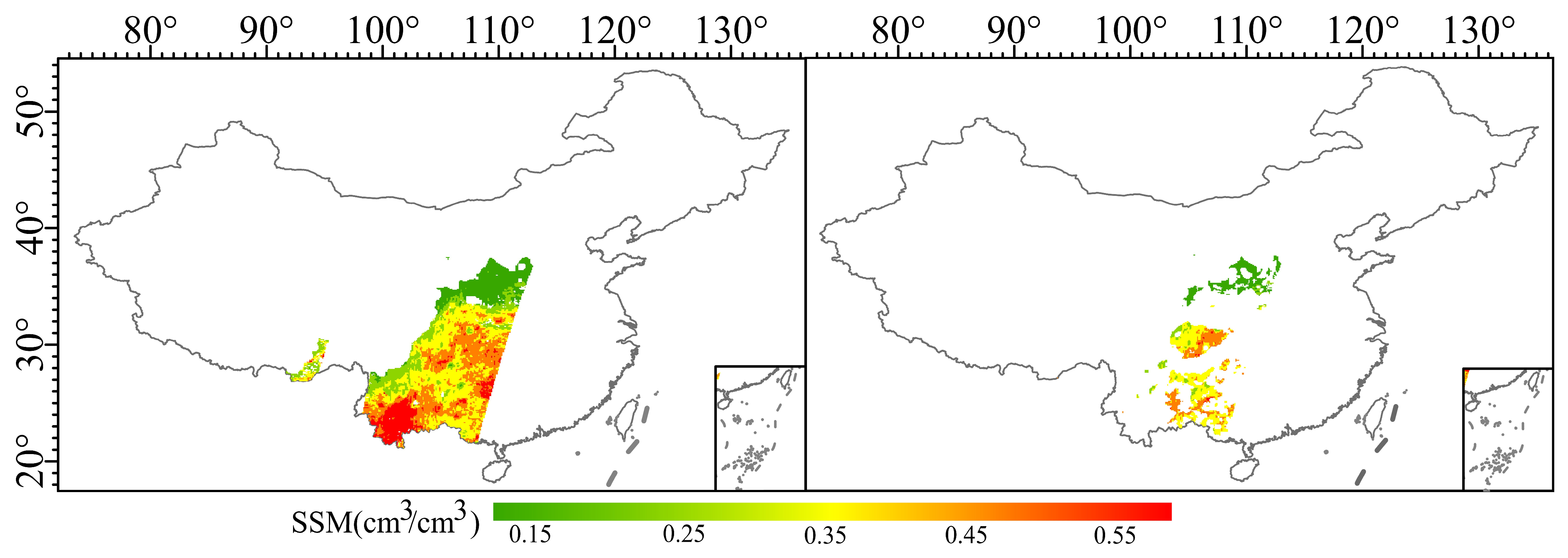
Remote sensing products typically incorporate a quality assurance (QA) band to store per-pixel quality metadata. This band employs bit-encoded flags, where individual or combined bits indicate specific quality conditions for each pixel. In this study, quality control was performed separately for the SMAP and vegetation index datasets. Given that SMAP SSM retrievals are influenced by land cover characteristics and canopy density, we excluded low-quality pixels during model training to avoid unstable gradient propagation in the neural network, which would otherwise impair model convergence and prediction accuracy. For vegetation indices, the MOD13A2 product was filtered using its QA bitmask to retain only noise-free and high-quality NDVI and EVI values. Since this study focuses exclusively on terrestrial soil moisture, NDVI and EVI values were further filtered to include only those within the range of 0 to 8000. All other values were masked as missing. A comparison of SMAP data before and after quality control is shown in Figure 2. In southern regions with dense vegetation cover, passive microwave observations from SMAP tend to overestimate soil moisture due to L-band signal attenuation caused by vegetation interaction.
While spatial quality control ensures reliable spatial representation, noise in the temporal dimension remains a challenge for long time series data. We then employed the SG filter for temporal smoothing the vegetation indices. This technique effectively reduces high-frequency noise while preserving the original trends and key inflection points in the data. The SG filter is based on a sliding window approach, where a polynomial is fitted to the data within the window and the center point is replaced by the fitted value. Compared to moving average methods, the SG filter better preserves the original shape and key dynamics of the data, minimizing distortion caused by high-frequency noise. The SG filter can be described by the following expression [49]:
Y j = i = m i = m C i Y j + i N ,
where Y j represents the smoothed value at time step j, Y j + i is the original time series value within the window, and C i is the weighting coefficient derived from polynomial fitting. The parameter N is the total number of points in the sliding window, which is typically an odd number to ensure a central value. The value m denotes half the window length, and a larger m results in smoother output curves. This filtering process enhances the temporal quality of the vegetation indices, improving the model’s ability to detect meaningful patterns in SSM dynamics.

2.2. Method

2.2.1. TsSMNet Model

The TsSMNet model is proposed as an improved residual autoencoder designed to reconstruct soil moisture from multi-source remote sensing data. It is adapted from the ResAutoNet framework and specifically optimized to reduce parameter complexity and overfitting risks associated with fully connected layers. In TsSMNet, the fully connected layers in the original architecture are replaced by Conv1D layers, which significantly reduce the number of trainable parameters. Beyond parameter efficiency, Conv1D layers effectively capture local dependencies within each spatial unit, making them particularly suitable for multi-source remote sensing data. In such applications, localized patterns often convey more meaningful information than global features, enhancing the model’s robustness to noisy inputs and improving overall predictive performance.
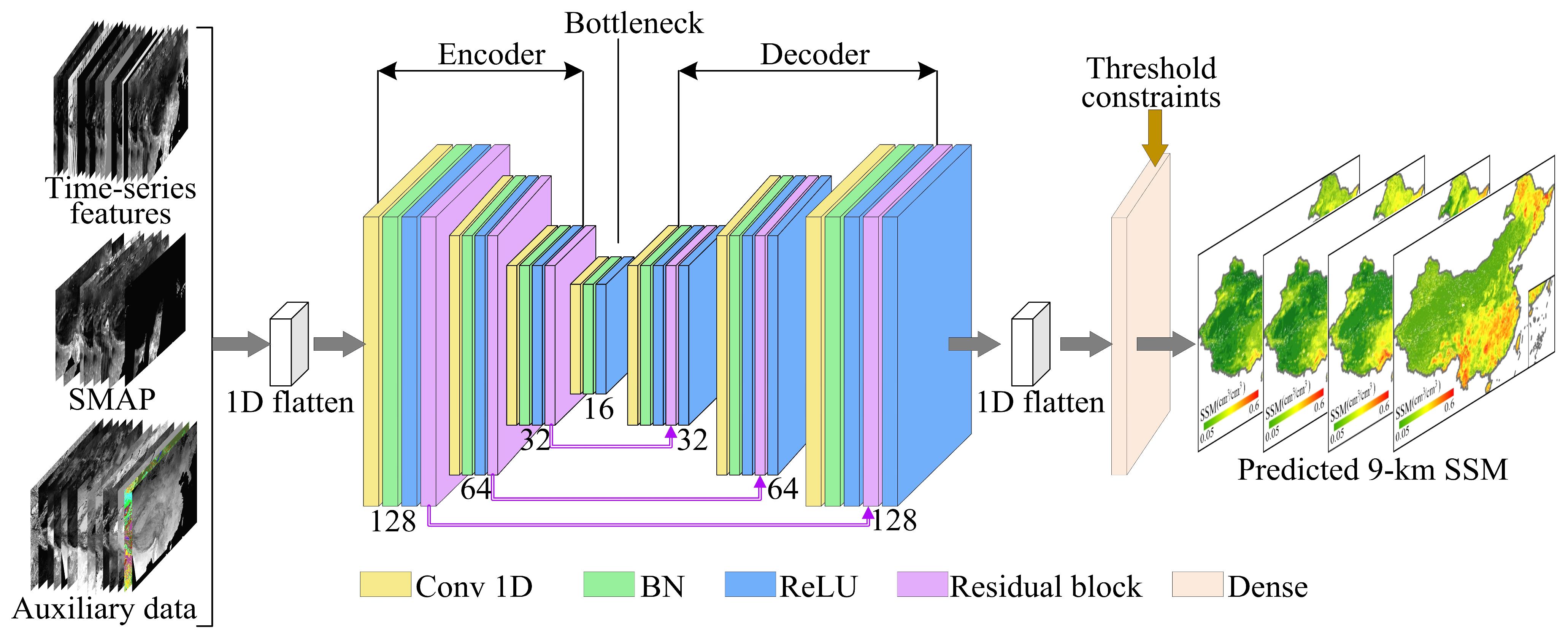
Similarly to ResAutoNet [50], TsSMNet adopts a symmetric hourglass structure composed of an encoder, a bottleneck layer, and a decoder. The encoder performs dimensionality reduction and feature extraction. The bottleneck layer transforms the encoded features, and the decoder reconstructs the output from these representations. Residual skip connections are introduced between corresponding encoder and decoder layers to preserve essential information and improve reconstruction accuracy. A fully connected layer at the end produces the initial SSM prediction, and a post-processing threshold constraint is applied to maintain physical consistency of the outputs. The number of encoder–decoder layers (three layers) follows the design of the original ResAutoNet framework, which has been shown to achieve stable and efficient reconstruction performance in remote sensing applications [50]. This configuration provides a balance between representational capacity and model simplicity, avoiding unnecessary depth that could lead to overfitting. The overall network structure is illustrated in Figure 3.
Each layer’s structure in TsSMNet is determined by a hyperparameter termed nodes, which defines the number of channels per layer and follows a symmetric format such as [i, j, …, k, …, j, i]. The list length is required to be odd to ensure the presence of a central bottleneck layer. Here, k indicates the number of channels in the bottleneck, while i and j refer to the outer and intermediate channel sizes in the encoder and decoder, respectively. In this study, the encoder comprises three Conv1D layers with 128, 64, and 32 channels, followed by a bottleneck layer with 16 channels. The decoder mirrors this structure in reverse order. This hierarchical design reflects the need for greater capacity at the input stage to extract relevant global patterns, with channel counts halved at each subsequent layer. The bottleneck size is typically set to half the smallest encoder layer [50].
The input data are first flattened across the spatial dimension and organized into a matrix with dimensions (n × h × d), where n denotes the total number of days (2557 daily records from 2016 to 2022), h denotes the number of features including both the dependent and independent variables, and d corresponds to the number of pixels in each image. These data are then reshaped into a format of (b × h × 1), where b equals n ×  d. Conv1D operations are applied along the feature dimension to capture local variable dependencies within spatial units.
The encoder consists of three convolutional layers, each followed by batch normalization (BN) and a Rectified Linear Unit (ReLU) activation. Each convolutional block in the Conv1D-based residual network consisted of a 1-D convolution layer (Conv1D) followed by batch normalization and ReLU activation. Each Conv1D layer in the encoder employs a kernel size of 3, stride = 1, and “same” padding to preserve the feature dimension, followed by batch normalization and a ReLU activation. The decoder mirrors the encoder with symmetric Conv1DTranspose layers (kernel size = 3, stride = 1, padding = “same”). A final 1 × 1 convolution is applied to project the decoded representation to the output channel. This configuration allows the model to extract spatially local feature patterns while maintaining alignment with the original feature dimension.
The transformation at the i-th layer is given by
E i = ReLU ( BN ( Conv ( E i 1 , W i , b i ) ) ) = f ( E i 1 , W i , b i ) ,
where E i denotes the output of the i-th layer ( i 1 ,   2 ,   3 ), W i , b i represent the layer’s weights and bias, and E 0 = X b h .
The ReLU activation function is defined as
R e L U x = m a x 0 , x .
Batch normalization normalizes layer inputs as follows:
x ^ = x μ B σ B 2 + ϵ ,
where μ B and σ B are the mean and standard deviation of the current batch, and ϵ is a small positive constant to prevent division by zero.
The bottleneck layer connects the encoder and decoder, can be expressed as
C = ReLU BN Conv E 3 , W c , b c = f E 3 , W c , b c .
The decoder reconstructs the encoded features back to the original input dimensions through layers with 32, 64, and 128 channels, which can be given by
H i = ReLU ( BN ( Conv ( D i 1 , W i , b i ) ) ) .
Here, H i is the output of the i-th layer convolution in the decoder layer, and D i 1 is the previous decoder output. The residual output for each decoder layer is computed as R i = E i + H i , where E i corresponds to the encoder output from the same level. After the final decoding layer, a fully connected layer is applied to obtain the prediction output. To ensure physical consistency, these predictions are clipped to a valid range 0 , θ s a t , where the upper limit θ s a t represents the soil’s saturated water content at each pixel. Specifically, θ s a t = m a x ( 1 ( ρ b / 2.65 ) , θ m a x h i s t ) , where θ m a x h i s t and ρ b are the historical maximum SMAP observation and soil bulk density (g cm−3) at that location, respectively. The empirical term 1 ( ρ b / 2.65 ) corresponds to the theoretical porosity of mineral soils, assuming an average particle density of 2.65 g cm−3. This formulation ensures that the saturation threshold reflects site-specific soil physical properties while also being constrained by observation-based extremes.
Note that this thresholding operation is applied only during inference to prevent physically implausible predictions and does not interfere with model optimization or gradient propagation.
The loss function plays a critical role in guiding the training of machine learning and deep learning models [51]. It measures the discrepancy between the predicted values and the ground truth. In this study, the root mean square error (RMSE) is adopted as the primary loss metric, with an added L2 regularization (weight decay) term to improve generalization. The loss function is defined as follows:
L θ w ,   b = 1 N i = 1 N Y i f θ w ,   b X i 2 + Ω θ w ,   b ,
where θ w ,   b denotes the model parameters including weights and biases, f θ w ,   b X i represents the model’s prediction for the i-th sample based on auxiliary variables X i , and Y i is the reference soil moisture from SMAP. The term Ω θ w ,   b represents the L2 penalty term used to reduce overfitting and stabilize the optimization process by discouraging excessively large weights.

2.2.2. Model Validation

To assess the performance of the proposed TsSMNet model in reconstructing SSM, comparative experiments were conducted using ResAutoNet, Transformer, RF and XGBoost as benchmark models. These four methods are widely applied in remote sensing and environmental prediction tasks due to their strong nonlinear modeling capabilities and robustness [25,26].
The ResAutoNet model, which ingeniously integrates residual connections into an autoencoder architecture, facilitates the training of deeper networks and enhances feature representation for more accurate image denoising tasks [52]. The Transformer, known for its parallelizable architecture and exceptional efficiency in handling long-range dependencies, has served as the foundational backbone for numerous state-of-the-art models in natural language processing and beyond [35]. The RF model operates by constructing an ensemble of decision trees trained on bootstrapped samples with random feature selection [53]. By averaging predictions across multiple independent trees, this ensemble design reduces the variance associated with any single tree and thus enhances the model’s generalization ability to unseen data. Moreover, RF provides a mechanism to assess the relative importance of input variables. XGBoost is an advanced implementation of gradient boosting. It incorporates regularization, efficient histogram-based computations, and parallelization [54]. These features enable it to handle missing values and high-dimensional sparse data efficiently, making it well-suited to capturing complex spatial and temporal dependencies.
Model performance was evaluated using five metrics, including correlation coefficient (r), RMSE, unbiased RMSE (ubRMSE), bias, and the slope of linear regression between ground observations and SSM products. Linear regression was performed for each SSM dataset, and the slope of each regression line was tested for statistical significance to assess whether predictions were consistent with observations. The correlation coefficient (dimensionless) reflects the strength of the linear relationship between predicted and observed values. RMSE, ubRMSE, and bias are expressed in volumetric soil moisture units (cm3/cm3), where RMSE indicates the overall prediction accuracy, ubRMSE quantifies the error structure independent of systematic bias, and bias measures the extent of consistent overestimation or underestimation. The slope of the regression line is also dimensionless and is used to evaluate the proportional consistency between model predictions and ground measurements. Four of the five metrics are computed as follows:
r = ( S S M i P S S M P ¯ ) ( S S M i T S S M T ¯ ) ( S S M i P S S M P ¯ ) 2 ( S S M i T S S M T ¯ ) 2 ,
Bias = 1 n i = 1 n ( S S M i P S S M i T ) ,
RMSE = 1 n i = 1 n ( S S M i P S S M i T ) 2 ,
ubRMSE = 1 n i = 1 n ( ( S S M i P S S M i T ) B i a s ) 2 ,
In these equations, S S M i P and S S M i T represent the predicted and observed SSM at location i, respectively. Their means are denoted by S S M P ¯ and S S M T ¯ , and n is the number of validation samples.

2.2.3. SSM Reconstruction Strategy

The reconstruction of SSM involves three main stages including data acquisition and preprocessing, model training for gap-filling, and performance evaluation of prediction outcomes. Figure 4 shows the procedure and methodology used in this study to reconstruct the SMAP SSM.
Initially, a comprehensive set of auxiliary variables is established through the integration of multisource remote sensing data and SMAP time-series products. Basic preprocessing steps were applied to each dataset according to its characteristics. For example, gap-filled Aqua MODIS LST data were reprojected to a common coordinate system, while vegetation indices were temporally resampled to daily values. Additional quality control and temporal smoothing were applied to SMAP data and vegetation datasets following the procedures described in Section 2.1.3 to ensure data reliability. Derived indices such as the TVDI were subsequently calculated from the preprocessed data. All datasets were clipped to the study area and spatially resampled to a uniform 9 km resolution to maintain consistency. To ensure robust feature extraction in regions with incomplete SSM observations, we constructed a multi-year averaged time series for each pixel before computing the 31 temporal descriptors. Specifically, for each day of the year (DOY), if a pixel had valid SSM observations in at least three out of the seven years (2016–2022), the multi-year mean value for that DOY was calculated from the available records. This process yielded a representative 365-day mean seasonal cycle for each pixel. Missing DOY values within this multi-year mean series were further interpolated using temporal smoothing (following the procedures described in Section 2.1.3) to ensure continuity. Subsequently, missing values in the original 7-year time series were filled according to the corresponding DOY values in the smoothed multi-year mean series. The gap-filled 7-year time series was then used to compute 31 temporal statistical features. After these preprocessing steps, 14 multisource auxiliary variables and 31 SMAP-based time-series features were compiled and standardized to a daily 9 km spatiotemporal resolution. Ground-based SSM measurements from the IMSN network are incorporated as reference data for validation.
Following preprocessing, five models are employed to perform daily reconstruction of SSM values, including ResAutoNet, Transformer, RF, XGBoost, and the proposed TsSMNet. To further evaluate the role of temporal features and the impact of collinearity, multiple training configurations were established: (1) TsSMNet trained “with all 45 features”, “without temporal variables”, and “with the reduced feature set after collinearity removal”; (2) ResAutoNet trained “with all features” and “with the reduced feature set after collinearity removal”; and (3) Transformer, RF, and XGBoost trained “with the reduced feature set after collinearity removal”. To assess the potential influence of multicollinearity among explanatory features, a variance inflation factor (VIF) analysis was conducted. Nine time-series statistical features with VIF values greater than 10 were identified and excluded to construct a “reduced feature set after collinearity removal” (Figure A1). The daily SMAP data were transformed into one-dimensional feature vectors. Only valid observations—defined as pixels with quality-controlled, non-missing SSM values and complete auxiliary feature inputs—were retained for analysis. These daily valid samples were randomly divided into training (80%) and validation (20%) subsets, ensuring that both sets represent the same spatial and temporal variability. Each observation corresponds to a specific pixel-day pair, and no minimum number of consecutive days was required for inclusion. Pixels containing missing values were allocated to the prediction set for subsequent gap-filling. The TsSMNet model is implemented using the Keras API within the TensorFlow framework. The training consists of 500 epochs with a batch size of 100. To enhance generalization and model efficiency, an early stopping strategy is applied to terminate training when performance no longer improves, while a learning rate scheduler (ReduceLROnPlateau) dynamically adjusts the learning rate. The ModelCheckpoint callback function is used to retain the best-performing model weights based on validation loss. Hyperparameters of Transformer, RF, and XGBoost models are tuned through Bayesian optimization. The Transformer model is configured with an embedding dimension of 80, 2 attention heads, 256 feed-forward hidden units, 3 transformer blocks, MLP units dimension of 80, a dropout rate of 0.1, and a learning rate of 0.0001727. For RF, the final parameters include a total of 500 trees, a maximum tree depth of 11, a minimum number of samples per split of 209, a minimum number of samples per leaf node of 104, a maximum features of 15, and bootstrap set to False. For XGBoost, the model is tuned with key hyperparameters including a learning rate of 0.01, 1000 trees, maximum tree depth of 9, L1 regularization of 4.52, L2 regularization of 0.45, gamma of 0.005, minimum child weight of 7, subsample ratio of 0.97, and feature sampling ratio of 0.79. All modeling and predictions were run on a computer with a CPU of 12th Gen Intel (R) Core (TM) i9-12900H (2.50 GHz) and 32.0 GB of memory.
After training, the models generate daily SSM predictions for all missing pixels. The accuracy of the reconstructed SSM is evaluated against ground-based IMSN observations and ESA CCI SSM using five statistical metrics, including r, RMSE, ubRMSE, bias and slope. Before comparing and validating with ESA CCI SSM, it is necessary to resample our SSM predictions into the same grid as ESA CCI SSM through average aggregation method, and filter the data of ESA CCI SSM to remove low-quality data.

3. Results

3.1. Training Performance and Feature Configuration Analysis of the TsSMNet Model

Table 3 summarizes the training and validation performance of all models under different feature configurations. To evaluate the influence of temporal information and multicollinearity, TsSMNet was trained under three feature configurations. By contrast, ResAutoNet, which relies solely on fully connected layers, was trained with both the full feature set and the reduced set after collinearity removal.
For TsSMNet, removing the highly collinear features slightly improved model performance, achieving the highest validation R2 (0.956) and the lowest validation loss (0.043). This indicates that addressing feature redundancy enhances model robustness and generalization. In contrast, excluding all temporal features caused a substantial decline in performance (validation R2 = 0.892), confirming that temporal statistical descriptors play a critical role in capturing short-term soil moisture variability. For ResAutoNet, comparable accuracy was observed between the full and reduced feature sets (validation R2 = 0.953 and 0.951, respectively). While this demonstrates its ability to maintain performance with lower-dimensional inputs, its overall validation R2 remains lower than that achieved by TsSMNet (0.956) under the optimized feature configuration. This performance gap highlights the limitation of the fully connected architecture in ResAutoNet compared to the Conv1D-based feature extraction in TsSMNet, which is more effective in capturing complex spatial patterns for accurate soil moisture reconstruction.
Figure 5 illustrates the training dynamics of the TsSMNet model over 500 epochs, displaying the evolution of both the loss function and the coefficient of determination (R2) on the training and validation sets. In the early stages of training (first 50 epochs), both the training loss (train_loss) and validation loss (val_loss) decrease rapidly, suggesting that the model quickly captures the nonlinear mapping between input features and target variables. After approximately 400 epochs, the training loss continues to decline and approaches near-zero values. Meanwhile, the validation loss also steadily decreases and stabilizes around the 450th epoch, indicating strong generalization performance without signs of overfitting. The R2 values for the training set (train_R2) and validation set (val_R2) show a similar trend. Both increase rapidly during the initial 30 epochs, and begin to stabilize after approximately 50 epochs. Notably, the training and validation R2 curves are closely aligned throughout the entire training process, which demonstrates excellent consistency between fitting and generalization ability. These results indicate that the TsSMNet model achieves stable convergence and demonstrates high accuracy and generalization capability.
Under the same reduced feature set without collinearity features, TsSMNet consistently outperformed Transformer, RF, and XGBoost models in validation accuracy and computational efficiency (Table 3). Although the Transformer achieved a comparable validation R2 (0.950), it required a substantially longer training time (24.6 h). In contrast, the ensemble models RF and XGBoost exhibited markedly lower performance (validation R2 = 0.828 and 0.878, respectively), reflecting their limited ability to capture complex nonlinear spatiotemporal dependencies. Overall, TsSMNet achieved the best balance between predictive accuracy, model stability, and computational cost, demonstrating its suitability for large-scale daily SSM reconstruction.

3.2. Reconstructed SSM Results

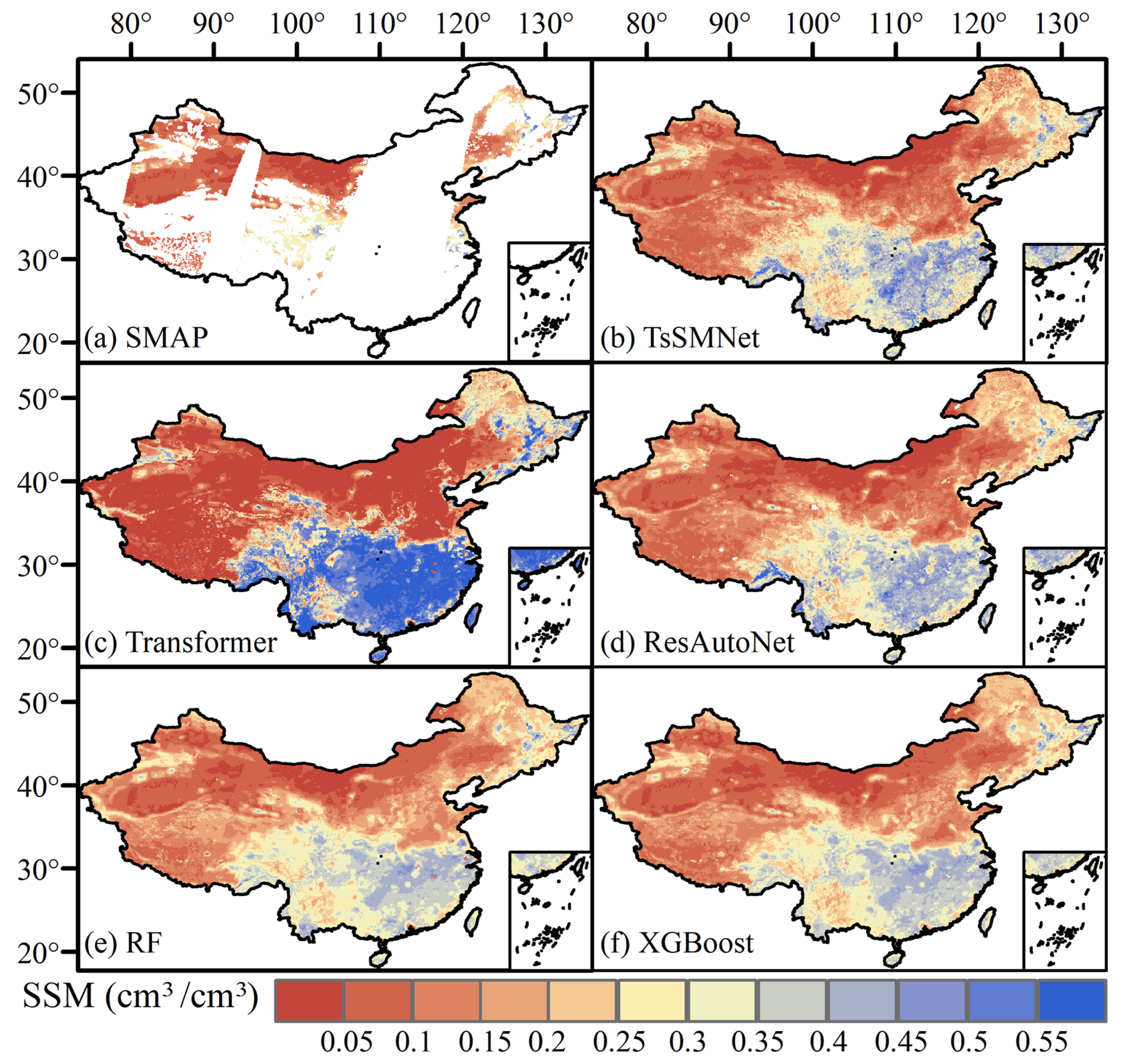
This study employed five models, including TsSMNet, ResAutoNet, Transformer, RF, and XGBoost, to reconstruct the missing SMAP SSM data across China from 2016 to 2022. The final output is a spatially continuous daily SSM dataset with a spatial resolution of 9 km. Figure 6 displays the 9 km SMAP SSM image in comparison with the reconstructed SSM predictions by five different models for 15 May 2019.
The overall spatial patterns produced by all five models demonstrate a reasonable ability to reproduce the SSM distribution across China. Higher values are observed in the southeast, while the northwest exhibits significantly lower moisture levels. This spatial pattern is broadly consistent with the distribution of precipitation, vegetation cover, and topography across the region. Although the overall spatial trend was consistent across models, differences emerged in their capacity to capture spatial details. The spatial distributions and SSM value ranges of RF and XGBoost were generally similar. However, compared to the other three models, both RF and XGBoost exhibited lower SSM estimates in humid regions and showed a tendency toward regional homogenization (Coefficient of Variation, CV = 0.55 and 0.58, respectively), failing to adequately capture fine-scale spatial heterogeneity. In contrast, the Transformer model results reflected a clearer spatial gradient—drier regions had lower SSM values, while more humid areas displayed higher moisture levels, better representing the overall moisture regime. TsSMNet and ResAutoNet produced similar spatial patterns and comparable SSM value ranges across different regions. Nevertheless, TsSMNet (CV = 0.64) demonstrated slightly richer spatial heterogeneity in SSM compared to ResAutoNet (CV = 0.63), more realistically reflecting local variations in soil moisture.
These findings indicate that while traditional machine learning models can partially reconstruct the missing SMAP data, they are less effective in capturing spatial details in humid regions. The Transformer model, though capable of capturing broad dry-wet patterns, is limited by its attention mechanism in reconstructing spatially continuous SSM fields with irregular gaps and fails to adequately represent localized moisture variability. Similarly, ResAutoNet, while reducing parameter redundancy compared to conventional fully connected networks, still lacks the capacity to capture fine-grained spatial textures due to its reliance on dense layers. In contrast, TsSMNet effectively overcomes these limitations by integrating Conv1D-based spatial feature extraction with temporal descriptors, enabling it to capture nonlinear spatiotemporal dynamics and produce SSM reconstructions with richer spatial heterogeneity and more consistent environmental fidelity.

3.3. Validation Through In Situ Observation and ESA CCI SSM

Table 4 summarizes the performance of TsSMNet, ResAutoNet, Transformer, RF, and XGBoost models, along with the original SMAP data, in predicting SSM at all in situ sites. Linear regression analysis confirmed that the slopes for all models were statistically significant (p < 0.05), indicating that the predicted SSM values are significantly linearly related to in situ observations. Among the five reconstruction models, TsSMNet yielded the best overall performance, with a slope of 0.605, a bias of −0.0115 cm3/cm3, RMSE of 0.093 cm3/cm3, and an r value of 0.66. This value of r is superior to that of Transformer (0.53), RF (0.64), XGBoost (0.61) and ResAutoNet (0.64), and is close to the SMAP original data (0.73). These results demonstrate that TsSMNet can not only fill data gaps effectively but also maintain consistency with ground observations, providing predictive performance close to the original SMAP measurements. In contrast, traditional machine learning models and Transformer model exhibited lower accuracy. The original SMAP data produced the highest r (0.73), indicating strong agreement with in situ observations. The similarity between RMSE and ubRMSE for both SMAP and TsSMNet confirms the minimal systematic bias for these two datasets. Compared to RF, XGBoost, Transformer and ResAutoNet, TsSMNet achieved a 9.7% average improvement in r, a 15.5% reduction in RMSE, a 10.6% reduction in ubRMSE, and a 5.3% increase in slope.
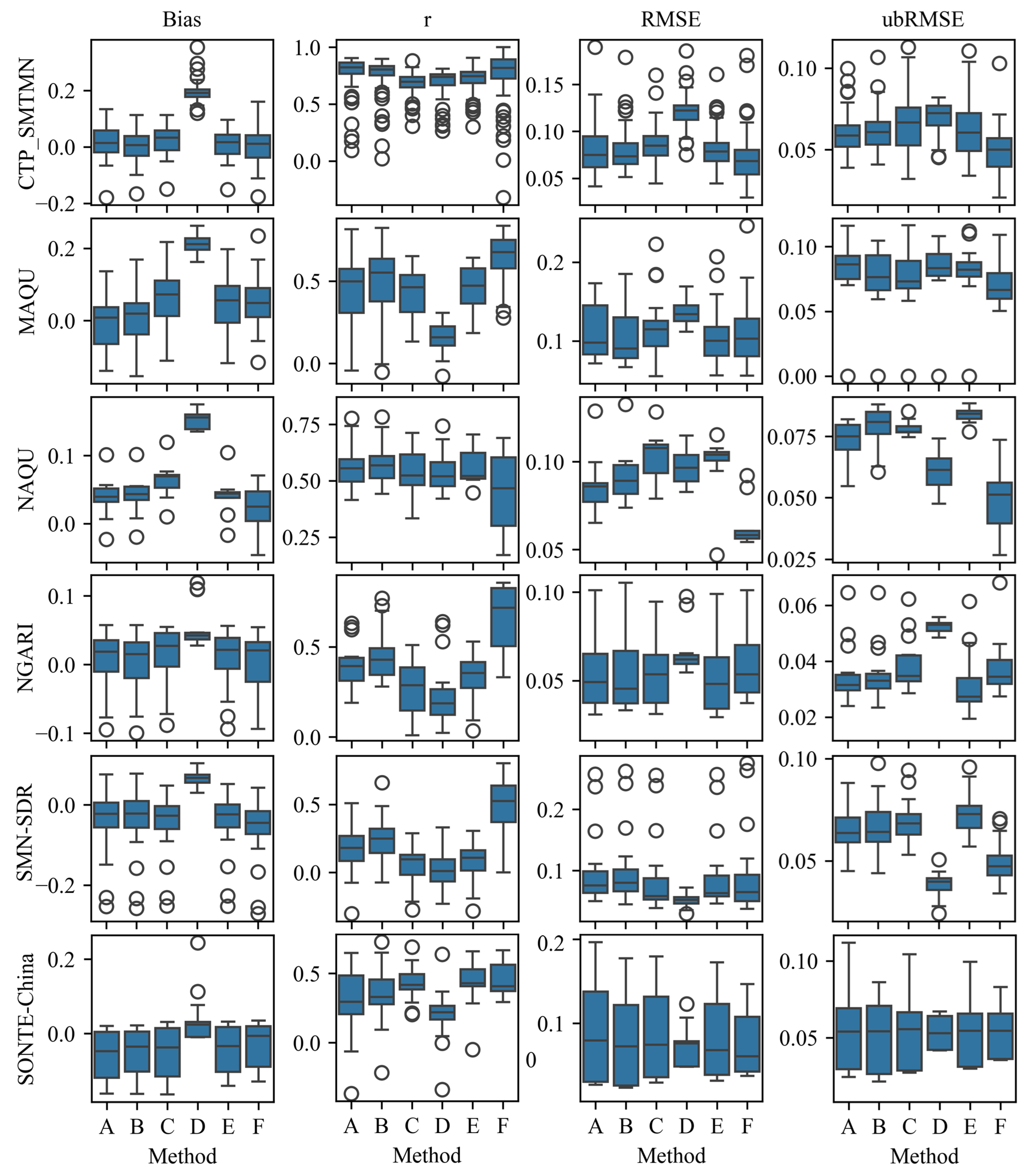
To further compare model performance, in situ validation was conducted for the five reconstructed products and original SMAP data across six observation networks. Figure 7 presents the distribution of key evaluation metrics at each network. Across the six networks, TsSMNet consistently outperformed Transformer, RF and XGBoost in most situations. While slight performance reductions were observed in isolated cases, TsSMNet generally achieved higher r values and more stable distributions. Transformer typically produced r values in the range of 0.3 to 0.5, rarely exceeding 0.5. In contrast, other five results achieved r values that frequently exceeded 0.5 and occasionally reached 0.8 at certain networks, such as CTP_SMTMN. These results further support the reliability and accuracy of TsSMNet for reconstructing satellite-based SSM product.
To assess the physical consistency of the reconstructed SSM product beyond sparse ground validation, we conducted a cross-validation using the ESA CCI SSM dataset (Figure 8). Across all valid grid cells nationwide (Count = 18,516,737), TsSMNet exhibited a strong agreement with ESA CCI (r = 0.734; RMSE = 0.0848 cm3/cm3). For comparison, the original SMAP product showed a higher consistency with ESA CCI (r = 0.801; RMSE = 0.0749 cm3/cm3), but this comparison was based only on SMAP-available pixels (N = 5,241,793), primarily located in regions with high data quality conditions. The fact that TsSMNet maintains a high correlation (r > 0.73) across the full spatial domain demonstrates that the reconstructed data preserve physically meaningful moisture gradients. We also analyzed the relationship between TsSMNet derived SSM and ESA CCI SSM in different climate zones (Figure 8c). Model performance shows clear spatial variation. The relationship between TsSMNet derived SSM and ESA CCI SSM is poor mainly in the humid subtropical climate and dry winter cold subarctic climate regions, while the relationship between the two is good in other climate regions.

4. Discussion

This section discusses the roles of temporal features and multi-source auxiliary data in enhancing SSM reconstruction performance. The analysis focuses on two aspects. First, it analyzes the role of temporal features using variable importance rankings from RF and XGBoost models. Second, it examines the performance of TsSMNet compared to a variant model trained without temporal features, referred to as SMNet. Additional findings and interpretations are also provided.

4.1. Importance and Selection of Temporal Features

Although RF and XGBoost demonstrate comparatively limited SSM reconstruction capabilities compared to TsSMNet, their variable importance analysis offers an objective way to assess the relative contribution of individual predictors. RF ranks features based on their ability to reduce mean squared error, while XGBoost determines feature importance based on cumulative gain and frequency in decision tree splits. As shown in Figure 9, the top seven features selected by both models are all derived from temporal statistical representations. These include the mean, median, CV, Q1, SegCorr, WHM, WGM, and WPM. Among them, WHM and WGM consistently exhibit the highest importance scores, particularly in XGBoost where their relative importance exceeds that of all other features. This result suggests that weighted average metrics are especially effective in capturing the temporal characteristics of SSM dynamics. In addition, the mean, median, and CV also appear among the most influential variables, indicating that central tendency and variability metrics are fundamental to reconstructing the overall behavior of the SSM time series.
However, the high importance of these features must be interpreted with caution due to the presence of multicollinearity. Many of these top-ranked features are mathematically related (e.g., WHM, WGM, and WPM are all variants of weighted means). To ensure model robustness and generalizability, we addressed this issue prior to training TsSMNet using the VIF, with a threshold of VIF > 10. The VIF analysis identified three distinct groups of highly collinear features: (1) measures of central tendency and magnitude: The Mean was highly collinear with RMS, Q1, WPM, WHM, WGM, and Median. This is expected as these metrics all capture the central value or overall magnitude of the time series. (2) measures of dispersion: The Std was collinear with MAD and IQR, as all three estimate data variability. (3) measures of serial dependence and energy: The AbsE was collinear with Sum and ACF. Consequently, we adopted a parsimonious strategy by keeping one feature from each collinear group (e.g., retaining the conceptually fundamental Mean and Std), resulting in the removal of 9 features (AbsE, ACF, MAD, Median, WGM, WHM, WPM, IQR, and RMS). This process explains why the final TsSMNet model was trained on a refined set without collinearity features. The superior performance of the model with this non-collinear feature set (as presented in Section 3.1) empirically confirms that mitigating multicollinearity is crucial for optimal performance, even if it involves removing some individually important features. The information conveyed by, for instance, WHM and WGM, is effectively captured by the retained Mean, leading to a more robust model.
Returning to the importance analysis, the CV ranks third and fourth in RF and XGBoost, respectively, highlighting its utility in capturing short-term fluctuations in hydrological responses. Previous studies have confirmed that temporal variability in SSM can affect retrieval accuracy under conditions of variable precipitation, evaporation, and surface fluxes [55,56]. The Q1 represents the lower distribution of SSM within the series and is particularly relevant for identifying relative drought conditions. The SegCorr quantifies local temporal consistency and may help detect short-term periodicity in SSM behavior.
Overall, temporal statistical features dominate the variable importance landscape in both models. These features effectively capture temporal dynamics that static variables (such as topography or soil type) cannot represent. Although the model inputs in this study also include remotely sensed variables such as LST, EVI, NDVI, and TVDI, these variables are instantaneous and cannot fully capture long-term SSM dynamics. In contrast, temporal features derived from historical sequences offer enhanced stability and provide complementary information to spatial predictors. This finding is consistent with previous research emphasizing the integration of temporal statistics for improved generalization in SSM modeling across diverse climatic and ecological zones [23].

4.2. Model Performance in the Absence of Temporal Features

To evaluate the specific contribution of temporal features, we compared TsSMNet against SMNet, which the latter excludes time-series features and uses only 14 multisource auxiliary variables. Figure 10 shows the reconstructed SSM maps at four representative dates across seasons in 2016, with the original SMAP retrievals as reference. Large data gaps in SMAP are observed over the Tibetan Plateau (high-altitude permafrost zones), northeast China (extremely low winter temperatures), and southwestern China (tropical forests), where environmental conditions impede reliable microwave signal retrieval.
While SMNet was able to fill spatial gaps, its predictions appear overly smoothed and lack seasonal or spatial variability. For instance, vast regions in the Tibetan Plateau (southwestern China), Inner Mongolia (northern China), and Xinjiang (northwestern China) exhibit uniform predicted values under SMNet. This limitation likely results from insufficient daily SMAP training pixels in cold seasons and the difficulty of learning complex relationships between auxiliary variables and SSM in such environments. By contrast, TsSMNet incorporates time-series features derived from multi-year SMAP records spanning 2016 to 2022. This allows the model to learn seasonal dynamics and long-term variability patterns. Visual results indicate that TsSMNet performs better in regions with complex terrain or dense vegetation. On a spring day, TsSMNet accurately reproduces the SSM conditions in high-altitude permafrost regions, avoiding the uniform and overly consistent predictions generated by SMNet. On a winter day, it captures clusters of high SSM in southern China, reflecting seasonal rainfall patterns. These improvements suggest that time-series features allow the model to capture historical SSM behavior and extrapolate under data-sparse conditions. In humid areas such as the middle and lower reaches of the Yangtze River, predictions from both models are more similar. This likely reflects the high predictive power of auxiliary variables in these regions, where surface temperature and vegetation indices already provide sufficient information. In humid regions like the middle and lower Yangtze River and southern China, SMNet and TsSMNet exhibit smaller prediction variations compared to other regions. This likely reflects the high predictive power of auxiliary variables in these regions, where the topographical and environmental variables (e.g., LST and vegetation indices) already provide sufficient information.
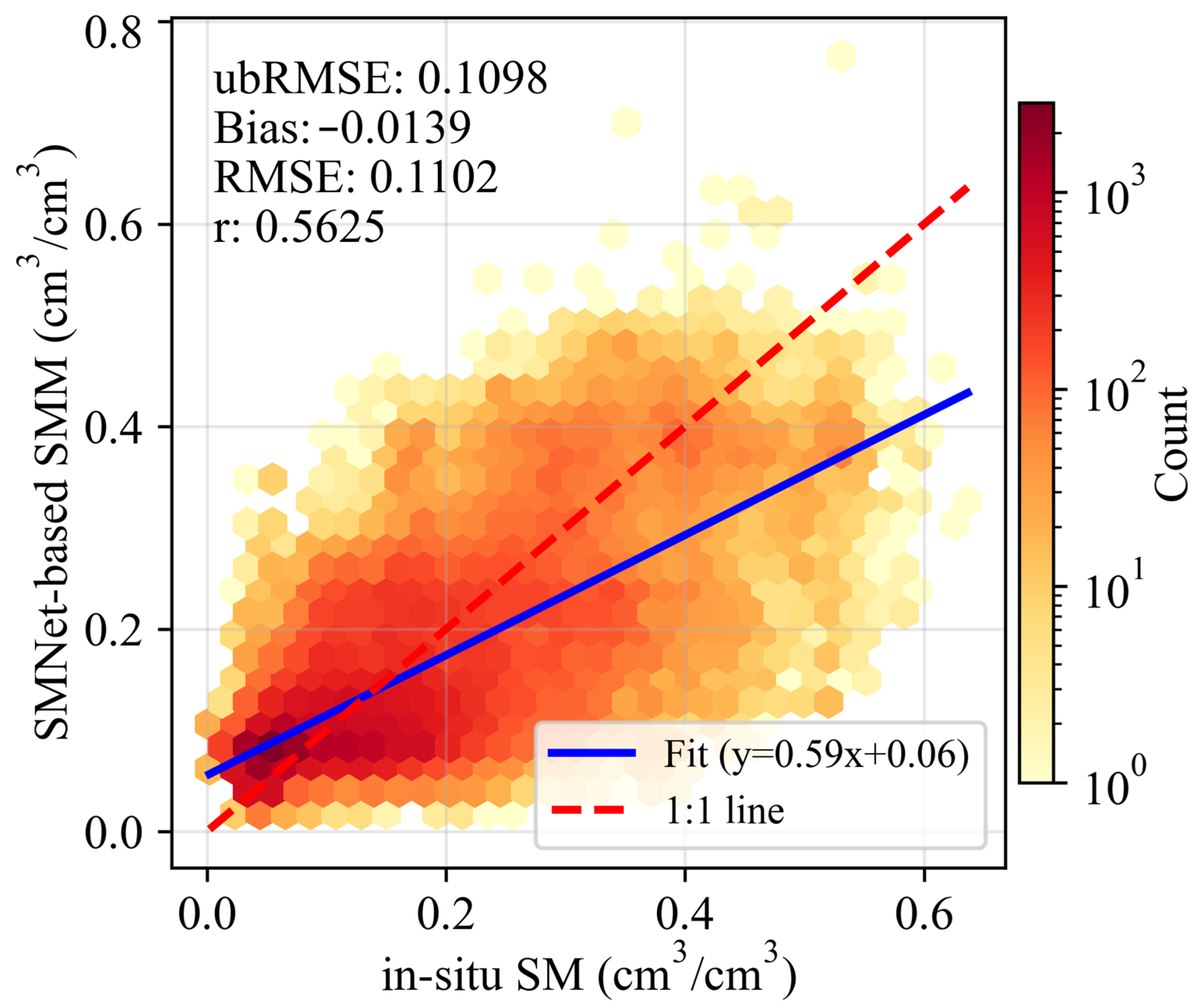
Evaluation against in situ observations further supports the added value of temporal features. Figure 11 shows a hexbin plot of SMNet predictions against in situ SM measurements. The figure reveals that SMNet achieves a slope of 0.59, a bias of −0.01 cm3/cm3, an RMSE of 0.11 cm3/cm3, an r value of 0.56, and an ubRMSE of 0.11 cm3/cm3. None of the evaluation metrics outperformed those of TsSMNet, suggesting that the exclusion of time-series features generally led to a reduction in model performance.
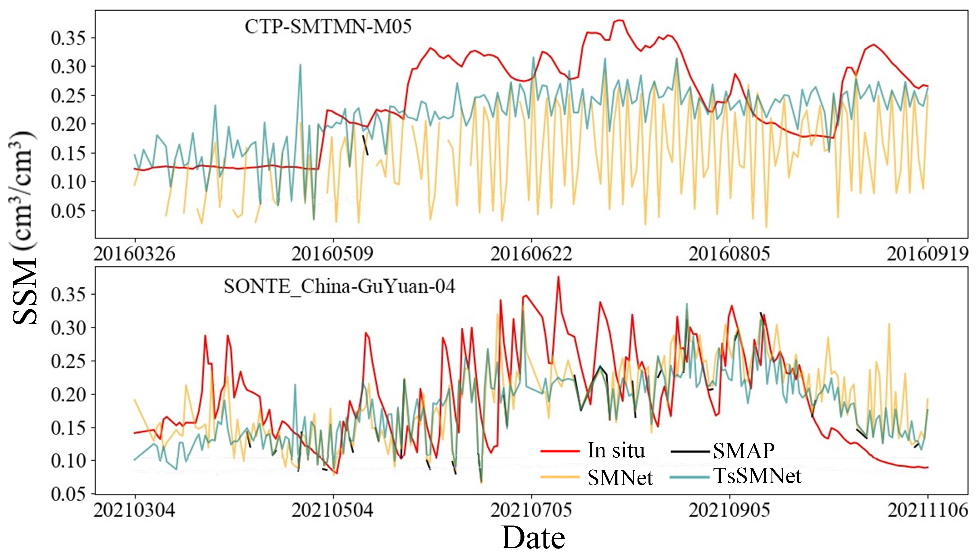
To assess the model’s ability to capture temporal dynamics, Figure 12 presents time series comparisons at two representative stations. These include M05 from the CTP_SMTMN network (91.725°E, 31.743°N) and GuYuan-04 from the SONTE-China network (115.6809°E, 41.76284°N). At the M05 site, SMNet significantly underestimates soil moisture and displays unstable fluctuations. TsSMNet shows closer agreement with in situ measurements. At the GuYuan-04 site, although SMNet performs relatively well during March 2021, TsSMNet generally tracks observed dynamics more accurately throughout the entire period, showing greater consistency. At the same time, the time series comparisons reveal that model performance varies under different environmental conditions. At the M05 site, which is located in a high-altitude meadow region of the Tibetan Plateau, TsSMNet improves upon SMNet but still shows noticeable deviations from in situ measurements. This may be related to freeze–thaw processes and the heterogeneous hydrothermal conditions that characterize alpine permafrost regions, which complicate the retrieval of soil moisture dynamics. In contrast, at the GuYuan-04 site, which represents a semi-arid shrubland, TsSMNet is able to reproduce observed variations more consistently. The relatively stable vegetation cover and climatic setting in this region may reduce uncertainties and allow the model to better capture temporal fluctuations. These differences from one site to another indicate that model accuracy can be influenced by regional climate regimes and land surface properties. The overall results demonstrate that incorporating time-series features enhances the model’s ability to reproduce seasonal and spatial variability, yielding more accurate and robust predictions. Although the current TsSMNet architecture balances parameter efficiency, feature extraction, and training stability, future work could explore alternative encoder–decoder designs to further improve performance, especially in regions with complex terrain.

4.3. Limitations and Research Prospects

Although TsSMNet has demonstrated strong performance in reconstructing soil moisture SSM over China, its applicability in other regions remains uncertain. The quality and spatial coverage of SMAP data vary across continents and climatic zones, and the model’s generalizability under diverse environmental conditions has not yet been validated. For example, validation at site locations revealed that only 23% of the sites exhibited an r with SMAP exceeding 0.8; in comparison, the corresponding TsSMNet model achieved this threshold (r > 0.8) at only 18.4% of the sites. The current validation relies on 198 stations from the ISMN. While these stations provide standardized observations across different climate and terrain conditions, their spatial distribution remains sparse relative to the continental scale, and temporal coverage is limited by available observation periods. This may affect the comprehensiveness of model evaluation, particularly in regions with complex topography or extreme climatic conditions. Moreover, although the TsSMNet–CCI correlation is slightly lower than SMAP–CCI when restricted to pixels with reliable SMAP retrievals, TsSMNet maintains strong satellite–satellite consistency over the full domain, including regions where SMAP observations are unavailable. This indicates that the reconstruction improves spatial continuity while preserving physical realism. Expanding the validation dataset, for example by incorporating additional in situ networks or performing cross-validation with other complementary satellite products, could improve the robustness of the performance assessment and better characterize model generalization under diverse environmental conditions. Such efforts would allow a more systematic assessment of regional differences in model performance and improve the robustness of the evaluation. In addition, applying the model to other continents and climate regimes could provide valuable insights into its transferability, potentially in combination with transfer learning or domain adaptation strategies to enhance robustness.
In terms of model structure, the use of Conv1D enables efficient extraction of localized feature dependencies but does not explicitly simulate sequential temporal dependencies. The input currently includes statistical summaries such as mean, CV, quintiles, and kurtosis. While these features provide information on historical trends and sudden events, they are computed over fixed periods and may not fully reflect rapid changes or extreme wet and dry conditions, potentially limiting the model’s predictive accuracy in highly dynamic situations. Incorporating temporal modeling architectures, such as recurrent neural networks or attention-based mechanisms, could enable the model to utilize sequential information more effectively and improve the representation of SSM dynamics across different climatic and ecological regions. These approaches are particularly beneficial for capturing short-term variability and rapidly evolving events, as supported by recent studies [57,58].
Moreover, while the constructed time-series features generally show good representativeness, their effectiveness may vary across ecological and climatic regions. For example, in arid zones or high-altitude areas, the relationships between climate drivers, vegetation, and SSM may differ significantly. Statistical analysis of bias across all sites revealed that the model tends to underestimate values at sites with relatively low vegetation coverage. This variability can reduce the reliability of statistical features in these regions. In addition, the extracted features were only standardized and no dimensionality reduction was performed, which may lead to redundancy and multicollinearity among variables. The temporal stability of these features across different seasons and regions was also not systematically evaluated. These limitations suggest that the current feature representation, although comprehensive, may still be sensitive to redundancy and environmental heterogeneity. Future work may explore the development of regionally adaptive temporal features and incorporate feature selection or stability analysis to improve model generalization under heterogeneous environmental conditions.
Although TsSMNet constrains predictions within physically valid limits by setting the upper bound of soil moisture to θ s a t = max(1 − ( ρ b /2.65), θ m a x h i s t ), ensuring consistency with soil porosity derived from bulk density, this treatment remains a post-processing correction. Such a thresholding approach does not influence model optimization and thus cannot enforce physical conservation during training. Consequently, the model may still yield temporally inconsistent or physically implausible values in regions with sparse observations or incomplete auxiliary data. We conducted a sensitivity test by varying the bulk density by ±10% to evaluate its effect on the saturation threshold. The resulting change in reconstructed SSM was within 0.003–0.02 cm3/cm3 for most regions, indicating that the post-processing constraint influences only extreme high-moisture conditions and does not affect the model training stage. Therefore, the threshold functions as a physical consistency safeguard rather than a parameter shaping the learned representation. Future research should aim to integrate physical constraints directly into the training process, for example by introducing differentiable regularization terms derived from soil water or energy balance equations. Such process-based priors could serve as soft physical constraints that enhance the model’s stability, physical consistency, and generalization across diverse environmental conditions [59].
In addition to retrieval accuracy, computational efficiency is essential for operational soil moisture monitoring. The TsSMNet model was trained on a workstation equipped with an Intel i9 CPU and 32 GB RAM, requiring approximately 24 h to complete one full-country model training. Once trained, the model generates daily SSM maps at 9 km resolution within about 4–6 min per day of data, depending on input data availability and I/O performance. This computational cost is moderate and comparable to commonly used machine learning–based satellite gap-filling workflows. More importantly, TsSMNet is applied in an inference-only manner during routine production, meaning that model training does not need to be repeated frequently. The model can be periodically updated (e.g., annually) to incorporate new observations or sensor calibrations, while daily SSM production can be fully automated. These characteristics suggest that TsSMNet is suitable for integration into long-term soil moisture data production pipelines.
Finally, although the model incorporates a range of auxiliary variables as input features, this may introduce redundant or less informative information. Incorporating attention mechanisms may help the model identify key variables and reduce the influence of irrelevant signals, which could enhance the prediction accuracy.

5. Conclusions

In this study, we successfully developed a spatially continuous SSM product based on SMAP data with a spatial resolution of 9 km, covering the period from January 2016 to December 2022 over China. By integrating multi-source remote sensing variables and statistical features derived from SMAP time series, we introduced the TsSMNet model, a residual autoencoder framework enhanced with convolutional feature extraction. The resulting SSM product was comprehensively evaluated through comparisons with the original SMAP retrievals, four benchmark machine learning models (ResAutoNet, Transformer, RF and XGBoost), and in situ observations. Validation results demonstrated that TsSMNet outperformed the four baseline models. Its estimates showed greater consistency with in situ measurements, and the evaluation metrics were closer to those obtained from SMAP compared to the other predictions. Variable importance analysis indicated that temporal predictors had a dominant role in improving model performance, highlighting the contribution of long-term soil moisture dynamics. Additional experiments with a variant of TsSMNet excluding time-series features further confirmed that the absence of temporal information significantly reduced predictive accuracy.
Overall, TsSMNet offers a promising approach for reconstructing long-term, spatially complete SSM dataset by combining convolutional spatial encoding and time-series statistical features. While a post-processing step ensures that outputs fall within physically reasonable ranges, the model lacks integrated physical constraints during training. Furthermore, its dependence on historical observations may limit its performance in regions experiencing rapid environmental changes or limited data availability. Future research should consider exploring physically guided learning strategies, investigating temporal generalization beyond the training period, and evaluating its scalability to other regions or global applications.

Author Contributions

Conceptualization, Y.J. and Y.L.; methodology, Y.L.; software, H.F.; validation, S.Z.; formal analysis, H.F.; investigation, Y.L.; resources, Y.J.; data curation, H.F.; writing—original draft preparation, Y.L. and H.F.; writing—review and editing, Y.L., Y.J. and S.Z.; visualization, Y.L. and Y.J.; supervision, Y.J.; project administration, Y.J.; funding acquisition, Y.J. and Y.L. All authors have read and agreed to the published version of the manuscript.

Funding

This work was supported in part by the National Natural Science Foundation of China under Grants 42201398 and 42001332, and the Startup Foundation for Introducing Talent of NUIST under Grant 2023r010.

Data Availability Statement

The 9 km daily SSM dataset over China, generated by TsSMNet model for the period from January 2016 to December 2022, is publicly available at https://doi.org/10.5281/zenodo.16419302 (accessed on 25 July 2025).

Acknowledgments

The authors would like to thank all data producers.

Conflicts of Interest

The authors declare no conflicts of interest.

Appendix A

To characterize the temporal dynamics of soil moisture time series, 31 statistical features were extracted from SMAP daily SSM observations during from 2016 to 2022. These features represent six categories of time series properties, namely central tendency, dispersion and variability, extremes and distributional characteristics, temporal dynamics, magnitude and energy, and count-based statistics. A complete list of the features, along with their abbreviations, definitions, and associated categories, is provided in Table A1.
Table A1. Description of the 31 statistical features derived from SMAP soil moisture time series.
CategoryFeature NameAbbreviationDefinition/Calculation
Central tendencyMeanMeanArithmetic average of the time series values
MedianMedianMiddle value of the series
Weighted harmonic meanWHMHarmonic mean weighted by observational weights
Weighted geometric meanWGMGeometric mean weighted by observational weights
Weighted power meanWPMPower mean with weighting
Dispersion and variabilityStandard deviationStdSquare root of variance
VarianceVarMean squared deviation from mean
Coefficient of variationCVStandard deviation divided by the mean
Mean absolute deviationMADAverage absolute difference from the mean
Median absolute deviationMeADMedian of absolute differences from the median
Interquartile rangeIQRDifference between the third quartile (Q3) and the first quartile (Q1)
Root mean squareRMSSquare root of the mean of squared values
Extremes and distributionMinimumMinLowest observed value
MaximumMaxHighest observed value
SkewnessSkewMeasure of asymmetry of the distribution
KurtosisKurtMeasure of peakedness of the distribution
First quartileQ125th percentile of the series
Sample entropySampEnQuantifies irregularity and unpredictability by comparing repeated patterns
Temporal dynamicsMean of successive differencesMeanDiffMean of differences between consecutive values
Median of successive differencesMedDiffMedian of differences between consecutive values
Mean absolute successive differenceMASDMean of absolute differences between consecutive values
Median absolute successive differenceMeASDMedian of absolute differences between consecutive values
AutocorrelationACFCorrelation of series with its lagged version
Second central derivative meanSecDerMeanMean of the second-order central differences, used to characterize the curvature and acceleration of changes in the time series.
Segment correlationSegCorrCorrelation between non-overlapping segments of the series, reflecting structural similarity and stability over time.
Peak-to-peak intervalP2PAverage interval between consecutive local maxima
Magnitude and energyAbsolute energyAbsESum of squared values
Sum of valuesSumTotal sum of series values
Sum of absolute differencesSADSum of absolute differences between consecutive values
Count-basedCount above meanCAMNumber of observations greater than mean
Count below meanCBMNumber of observations less than mean
To assess multicollinearity, a variance inflation factor (VIF) analysis was conducted, which identified nine time-series features (i.e., AbsE, ACF, MAD, Median, WGM, WHM, WPM, IQR, and RMS) with VIF values greater than 10 for exclusion, leading to the reduced feature set without collinearity features as shown in Figure A1.
Figure A1. Multi-collinearity analysis among explanatory features based on variance inflation factor (VIF).
Remotesensing 17 03729 g0a1

References

  1. Zhang, M.; Zhang, D.; Jin, Y.; Wan, X.; Ge, Y. Evolution of Soil Moisture Mapping from Statistical Models to Integrated Mechanistic and Geoscience-Aware Approaches. Inform. Geogr. 2025, 1, 100005. [Google Scholar] [CrossRef]
  2. Ge, Y.; Hu, S.; Song, Y.Z.; Zheng, H.; Liu, Y.S.; Ye, X.Y.; Ma, T.; Liu, M.X.; Zhou, C.H. Sustainable poverty reduction models for the coordinated development of the social economy and environment in China. Sci. Bull. 2023, 68, 2236–2246. [Google Scholar] [CrossRef]
  3. Narasimhan, B.; Srinivasan, R.; Arnold, J.G.; Di Luzio, M. Estimation of Long-Term Soil Moisture Using a Distributed Pa-Rameter Hydrologic Model and Verification Using Remotely Sensed Data. Trans. ASAE 2005, 48, 1101–1113. [Google Scholar] [CrossRef]
  4. Chakrabarti, S.; Bongiovanni, T.; Judge, J.; Nagarajan, K.; Principe, J.C. Downscaling Satellite-Based Soil Moisture in Heterogeneous Regions Using High-Resolution Remote Sensing Products and Information Theory: A Synthetic Study. IEEE Trans. Geosci. Remote Sens. 2015, 53, 85–101. [Google Scholar] [CrossRef]
  5. Peng, J.; Loew, A.; Merlin, O.; Verhoest, N.E.C. A Review of Spatial Downscaling of Satellite Remotely Sensed Soil Moisture. Rev. Geophys. 2017, 55, 341–366. [Google Scholar] [CrossRef]
  6. Zhao, W.; Wen, F.P.; Cai, J.F. Methods, Progresses, and Challenges of Passive Microwave Soil Moisture Spatial Downscaling. Nat. Remote Sens. Bull. 2022, 26, 1699–1722. [Google Scholar] [CrossRef]
  7. Yang, Z.; He, Q.; Miao, S.; Wei, F.; Yu, M. Surface Soil Moisture Retrieval of China Using Multi-Source Data and Ensemble Learning. Remote Sens. 2023, 15, 2786. [Google Scholar] [CrossRef]
  8. Das, N.N.; Entekhabi, D.; Dunbar, R.S.; Chaubell, M.J.; Colliander, A.; Yueh, S.; Jagdhuber, T.; Chen, F.; Crow, W.; O’Neill, P.E.; et al. The SMAP and Copernicus Sentinel 1A/B microwave active-passive high resolution surface soil moisture product. Remote Sens. Environ. 2019, 233, 111380. [Google Scholar] [CrossRef]
  9. Colliander, A.; Reichle, R.H.; Crow, W.T.; Cosh, M.H.; Chen, F.; Chan, S.; Das, N.N.; Bindlish, R.; Chaubell, J.; Kim, S.; et al. Validation of Soil Moisture Data Products from the NASA SMAP Mission. IEEE J. Sel. Top. Appl. Earth Obs. Remote Sens. 2022, 15, 364–392. [Google Scholar] [CrossRef]
  10. Setti, P.T.; Tabibi, S. Enhancing Soil Moisture Estimates Through the Fusion of SMAP and GNSS-R Data at 3-Km Resolution for Daily Mapping. IEEE J. Sel. Top. Appl. Earth Obs. Remote Sens. 2025, 18, 5303–5316. [Google Scholar] [CrossRef]
  11. Xing, C.; Chen, N.; Zhang, X.; Gong, J. A Machine Learning Based Reconstruction Method for Satellite Remote Sensing of Soil Moisture Images with In Situ Observations. Remote Sens. 2017, 9, 484. [Google Scholar] [CrossRef]
  12. Usowicz, B.; Lipiec, J.; Łukowski, M.; Słomiński, J. Improvement of Spatial Interpolation of Precipitation Distribution Using Cokriging Incorporating Rain-Gauge and Satellite (SMOS) Soil Moisture Data. Remote Sens. 2021, 13, 1039. [Google Scholar] [CrossRef]
  13. Liu, C.Y.; Yao, L.; Jing, W.; Di, L.; Yang, J.; Li, Y. Comparison of Two Satellite-Based Soil Moisture Reconstruction Algorithms: A Case Study in the State of Oklahoma, USA. J. Hydrol. 2020, 590, 125406. [Google Scholar] [CrossRef]
  14. Cui, Y.; Chen, X.; Xiong, W.; He, L.; Lv, F.; Fan, W.; Luo, Z.; Hong, Y. A Soil Moisture Spatial and Temporal Resolution Improving Algorithm Based on Multi-Source Remote Sensing Data and GRNN Model. Remote Sens. 2020, 12, 455. [Google Scholar] [CrossRef]
  15. Xiao, Z.; Jiang, L.; Zhu, Z.; Wang, J.; Du, J. Spatially and Temporally Complete Satellite Soil Moisture Data Based on a Data Assimilation Method. Remote Sens. 2016, 8, 49. [Google Scholar] [CrossRef]
  16. Nadeem, A.A.; Zha, Y.; Shi, L.; Ali, S.; Wang, X.; Zafar, Z.; Afzal, Z.; Tariq, M.A.U.R. Spatial Downscaling and Gap-Filling of SMAP Soil Moisture to High Resolution Using MODIS Surface Variables and Machine Learning Approaches over ShanDian River Basin, China. Remote Sens. 2023, 15, 812. [Google Scholar] [CrossRef]
  17. Ding, T.; Zhao, W.; Yang, Y. Addressing spatial gaps in ESA CCI soil moisture product: A hierarchical reconstruction approach using deep learning model. Int. J. Appl. Earth Obs. Geoinf. 2024, 132, 104003. [Google Scholar] [CrossRef]
  18. Llamas, R.M.; Guevara, M.; Rorabaugh, D.; Taufer, M.; Vargas, R. Spatial Gap-Filling of ESA CCI Satellite-Derived Soil Moisture Based on Geostatistical Techniques and Multiple Regression. Remote Sens. 2020, 12, 665. [Google Scholar] [CrossRef]
  19. Tong, C.; Wang, H.; Magagi, R.; Goita, K.; Wang, K. Spatial Gap-Filling of SMAP Soil Moisture Pixels over Tibetan Plateau via Machine Learning Versus Geostatistics. IEEE J. Sel. Top. Appl. Earth Obs. Remote Sens. 2021, 14, 9899–9912. [Google Scholar] [CrossRef]
  20. Sun, H.; Xu, Q. Evaluating Machine Learning and Geostatistical Methods for Spatial Gap-Filling of Monthly ESA CCI Soil Moisture in China. Remote Sens. 2021, 13, 2848. [Google Scholar] [CrossRef]
  21. Zhang, C.; Zeng, J.; Shi, P.; Ma, H.; Letu, H.; Zhang, X.; Wang, P.; Bi, H.; Rong, J. Global-Scale Gap Filling of Satellite Soil Moisture Products: Methods and Validation. J. Hydrol. 2025, 653, 132762. [Google Scholar] [CrossRef]
  22. Liu, K.; Li, X.; Wang, S.; Zhang, H. A Robust Gap-Filling Approach for European Space Agency Climate Change Initiative (ESA CCI) Soil Moisture Integrating Satellite Observations, Model-Driven Knowledge, and Spatiotemporal Machine Learning. Hydrol. Earth Syst. Sci. 2023, 27, 577–598. [Google Scholar] [CrossRef]
  23. Yang, H.; Wang, Q. Reconstruction of a Spatially Seamless, Daily SMAP (SSD_SMAP) Surface Soil Moisture Dataset from 2015 to 2021. J. Hydrol. 2023, 621, 129579. [Google Scholar] [CrossRef]
  24. Shangguan, Y.; Min, X.; Shi, Z. Gap Filling of the ESA CCI Soil Moisture Data Using a Spatiotemporal Attention-Based Residual Deep Network. IEEE J. Sel. Top. Appl. Earth Obs. Remote Sens. 2023, 16, 5344–5354. [Google Scholar] [CrossRef]
  25. Zhang, Y.; Liang, S.; Zhu, Z.; Ma, H.; He, T. Soil Moisture Content Retrieval from Landsat 8 Data Using Ensemble Learning. ISPRS J. Photogramm. Remote Sens. 2022, 185, 32–47. [Google Scholar] [CrossRef]
  26. Jia, Y.; Xiao, Z.; Jin, S.; Yan, Q.; Jin, Y.; Li, W. Improving CYGNSS-Based Soil Moisture Coverage through Autocorrelation and Machine Learning-Aided Method. IEEE J. Sel. Top. Appl. Earth Obs. Remote Sens. 2024, 17, 12554–12566. [Google Scholar] [CrossRef]
  27. Hu, Z.; Chai, L.; Crow, W.T.; Liu, S.; Zhu, Z.; Zhou, J.; Qu, Y.; Liu, J.; Yang, S.; Lu, Z. Applying a Wavelet Transform Technique to Optimize General Fitting Models for SM Analysis: A Case Study in Downscaling over the Qinghai–Tibet Plateau. Remote Sens. 2022, 14, 3063. [Google Scholar] [CrossRef]
  28. Xing, Z.; Fan, L.; Zhao, L.; De Lannoy, G.; Frappart, F.; Peng, J.; Li, X.; Zeng, J.; Al-Yaari, A.; Yang, K.; et al. A first assessment of satellite and reanalysis estimates of surface and root-zone soil moisture over the permafrost region of Qinghai-Tibet Plateau. Remote Sens. Environ. 2021, 265, 112666. [Google Scholar] [CrossRef]
  29. Yang, H.; Wang, Q.; Ma, X.; Liu, W.; Liu, H. Digital Soil Mapping Based on Fine Temporal Resolution Landsat Data Produced by Spatiotemporal Fusion. IEEE J. Sel. Top. Appl. Earth Obs. Remote Sens. 2023, 16, 3905–3914. [Google Scholar] [CrossRef]
  30. Jiang, M.; Qiu, T.; Wang, T.; Zeng, C.; Zhang, B.; Shen, H. Seamless Global Daily Soil Moisture Mapping using Deep Learning Based Spatiotemporal Fusion. Int. J. Appl. Earth Obs. Geoinf. 2025, 139, 104517. [Google Scholar] [CrossRef]
  31. Li, Q.; Li, Z.; Shangguan, W.; Wang, X.; Li, L.; Yu, F. Improving Soil Moisture Prediction using a Novel Encoder-Decoder Model with Residual Learning. Comput. Electron. Agric. 2022, 195, 106816. [Google Scholar] [CrossRef]
  32. Xiong, Z.; Zhang, Z.; Gui, H.; Chen, X.; Hu, S.; Gao, L.; Yang, H.; Qiu, J.; Xin, Q. A Meteorology-Driven Transformer Network to Predict Soil Moisture for Agriculture Drought Forecasting. IEEE Trans. Geosci. Remote Sens. 2025, 63, 4405818. [Google Scholar] [CrossRef]
  33. Gao, P.; Fang, J.; He, J.; Ma, S.; Wen, G.; Li, Z. GRU–Transformer Hybrid Model for GNSS/INS Integration in Orchard Environments. Agriculture 2025, 15, 1135. [Google Scholar] [CrossRef]
  34. Zhang, Y.; Liang, S.; Ma, H.; He, T.; Tian, F.; Zhang, G.; Xu, J. A Seamless Global Daily 5 km Soil Moisture Product from 1982 to 2021 using AVHRR Satellite Data and An Attention-Based Deep Learning Model. Earth Syst. Sci. Data Discuss 2025, 17, 1–39. [Google Scholar] [CrossRef]
  35. Liu, Y.; Xin, Y.; Yin, C. A Transformer-Based Method to Simulate Multi-Scale Soil Moisture. J. Hydrol. 2025, 655, 132900. [Google Scholar] [CrossRef]
  36. Dabboor, M.; Atteia, G.; Meshoul, S.; Alayed, W. Deep Learning-Based Framework for Soil Moisture Content Retrieval of Bare Soil from Satellite Data. Remote Sens. 2023, 15, 1916. [Google Scholar] [CrossRef]
  37. Shi, C.; Zhang, Z.; Xiong, S.; Zhang, W. Enhancing Global Surface Soil Moisture Estimation from ESA CCI and SMAP Product with Conditional Variational Auto-Encoder. IEEE J. Sel. Top. Appl. Earth Obs. Remote Sens. 2024, 17, 9337–9359. [Google Scholar] [CrossRef]
  38. Zhang, Z.; Xu, W.; Qin, Q.; Long, Z. Downscaling Solar-Induced Chlorophyll Fluorescence Based on Convolutional Neural Network Method to Monitor Agricultural Drought. IEEE Trans. Geosci. Remote Sens. 2021, 59, 1012–1028. [Google Scholar] [CrossRef]
  39. Hu, P.; Pan, X.; Yang, Y.; Dai, Y.; Chen, Y. A Two-Stage Hierarchical Spatiotemporal Fusion Network for Land Surface Temperature with Transformer. IEEE Trans. Geosci. Remote Sens. 2025, 63, 5002320. [Google Scholar] [CrossRef]
  40. Ge, Y.; Zhang, L.; Han, Y.; Zhang, D.; Yang, W.J.; Feng, L.; Dong, J.W.; Wang, S.P.; Peng, S.M.; Fang, C.Y. Enhancing water security in lake basins through geographic intelligence technology. Sci. Bull. 2025, 70, 2047–2050. [Google Scholar] [CrossRef]
  41. Egeonu, D.; Jia, B. Performance Evaluation and Comparison of Deep Neural Network Models for African Soil Properties Prediction. Commun. Soil Sci. Plant Anal. 2024, 55, 2799–2820. [Google Scholar] [CrossRef]
  42. Liu, N.; Wan, L.; Zhang, Y.; Zhou, T.; Huo, H.; Fang, T. Exploiting Convolutional Neural Networks with Deeply Local Description for Remote Sensing Image Classification. IEEE Access 2018, 6, 11215–11228. [Google Scholar] [CrossRef]
  43. Entekhabi, D.; Njoku, E.G.; O’Neill, P.E.; Kellogg, K.H.; Crow, W.T.; Edelstein, W.N.; Entin, J.K.; Goodman, S.D.; Jackson, T.J.; Johnson, J.; et al. The Soil Moisture Active Passive (SMAP) Mission. Proc. IEEE 2010, 98, 704–716. [Google Scholar] [CrossRef]
  44. Dorigo, W.; Wagner, W.; Albergel, C.; Albrecht, F.; Balsamo, G.; Brocca, L.; Chung, D.; Ertl, M.; Forkel, M.; Gruber, A.; et al. ESA CCI Soil Moisture for improved Earth system understanding: State-of-the art and future directions. Remote Sens. Environ. 2017, 15, 185–215. [Google Scholar] [CrossRef]
  45. Zhang, X.; Zhou, J.; Liang, S.; Wang, D. A Practical Reanalysis Data and Thermal Infrared Remote Sensing Data Merging (RTM) Method for Reconstruction of a 1-Km All-Weather Land Surface Temperature. Remote Sens. Environ. 2021, 260, 112437. [Google Scholar] [CrossRef]
  46. Xia, L.; Song, X.; Leng, P.; Wang, Y.; Hao, Y.; Wang, Y. A Comparison of Two Methods for Estimating Surface Soil Moisture Based on the Triangle Model Using Optical/Thermal Infrared Remote Sensing over the Source Area of the Yellow River. Int. J. Remote Sens. 2018, 40, 2120–2137. [Google Scholar] [CrossRef]
  47. Hengl, T.; Consoli, D.; Tian, X.; Nauman, T.W.; Nussbaum, M.; Isik, M.S.; Parente, L.; Ho, Y.-F.; Simoes, R.; Gupta, S.; et al. OpenLandMap-SoilDB: Global Soil Information at 30 m Spatial Resolution for 2000–2022+ Based on Spatiotemporal Machine Learning and Harmonized Legacy Soil Samples and Observations. Earth Syst. Sci. Data Discuss. 2025, 2025, 1–66. [Google Scholar] [CrossRef]
  48. Dorigo, W.; Himmelbauer, I.; Aberer, D.; Schremmer, L.; Petrakovic, I.; Zappa, L. The International Soil Moisture Network: Serving Earth System Science for over a Decade. Hydrol. Earth Syst. Sci. 2021, 25, 5749–5804. [Google Scholar] [CrossRef]
  49. Cao, R.; Chen, Y.; Shen, M.; Chen, J.; Zhou, J.; Wang, C.; Yang, W. A Simple Method to Improve the Quality of NDVI Time-Series Data by Integrating Spatiotemporal Information with the Savitzky-Golay Filter. Remote Sens. Environ. 2018, 217, 244–257. [Google Scholar] [CrossRef]
  50. Chen, Y.; Wu, G.; Ge, Y.; Xu, Z. Mapping Gridded Gross Domestic Product Distribution of China Using Deep Learning with Multiple Geospatial Big Data. IEEE J. Sel. Top. Appl. Earth Obs. Remote Sens. 2022, 15, 1791–1802. [Google Scholar] [CrossRef]
  51. Li, L.; Fang, Y.; Wu, J.; Wang, J.; Ge, Y. Encoder–Decoder Full Residual Deep Networks for Robust Regression and Spatio-temporal Estimation. IEEE Trans. Neural Netw. Learn. Syst. 2021, 32, 4217–4230. [Google Scholar] [CrossRef] [PubMed]
  52. Terven, J.; Cordova-Esparza, D.M.; Romero-González, J.A.; Ramírez-Pedraza, A.; Chávez-Urbiola, E.A. A Comprehensive Survey of Loss Functions and Metrics in Deep Learning. Artif. Intell. Rev. 2025, 58, 195. [Google Scholar] [CrossRef]
  53. Breiman, L. Random Forests. Mach. Learn. 2001, 45, 5–32. [Google Scholar] [CrossRef]
  54. Chen, T.; Guestrin, C. Xgboost: A scalable tree boosting system. In Proceedings of the 22nd ACM Sigkdd International Conference on Knowledge Discovery and Data Mining, San Francisco, CA, USA, 13–17 August 2016; pp. 785–794. [Google Scholar] [CrossRef]
  55. Li, Z.-L.; Leng, P.; Zhou, C.; Chen, K.-S.; Zhou, F.-C.; Shang, G.-F. Soil Moisture Retrieval from Remote Sensing Measurements: Current Knowledge and Directions for the Future. Earth-Sci. Rev. 2021, 218, 103673. [Google Scholar] [CrossRef]
  56. Le, M.S.; Liou, Y.-A. Spatio-Temporal Assessment of Surface Moisture and Evapotranspiration Variability Using Remote Sensing Techniques. Remote Sens. 2021, 13, 1667. [Google Scholar] [CrossRef]
  57. Wang, Q.; You, Y.; Yang, H.; Xu, R.; Zhang, H.K.; Lu, P.; Tong, X. A TCN-Transformer Parallel Model for Reconstruction of a Global, Daily, Spatially Seamless FY-3B Soil Moisture Dataset. Remote Sens. Environ. 2025, 328, 114841. [Google Scholar] [CrossRef]
  58. Li, X.; Zhang, Z.; Li, Q.; Zhu, J. Enhancing Soil Moisture Forecasting Accuracy with REDF-LSTM: Integrating Residual En-Decoding and Feature Attention Mechanisms. Water 2024, 16, 1376. [Google Scholar] [CrossRef]
  59. Li, L.; Dai, Y.J.; Wei, Z.W.; Wei, S.G.; Wei, N.; Zhang, Y.G.; Li, Q.L.; Li, X.X. Enhancing Deep Learning Soil Moisture Forecasting Models by Integrating Physics-based Models. Adv. Atmos. Sci. 2024, 41, 1326–1341. [Google Scholar] [CrossRef]
Figure 1. Study area and distribution of soil moisture observation sites.
Remotesensing 17 03729 g001
Figure 2. Comparison of original and quality-controlled SMAP SSM data on 1 September 2016.
Remotesensing 17 03729 g002
Figure 3. The TsSMNet model structure.
Remotesensing 17 03729 g003
Figure 4. The reconstruction strategy for SMAP SSM.
Remotesensing 17 03729 g004
Figure 5. Loss and R2 trends of TsSMNet model on training and validation sets over 500 epochs.
Remotesensing 17 03729 g005
Figure 6. Comparison of 9 km SMAP SSM and reconstructed SSM by five models on 15 May 2019.
Remotesensing 17 03729 g006
Figure 7. Boxplots of evaluation metrics for original SMAP and five reconstructed SSM products across six in situ soil moisture networks. A corresponds to ResAutoNet, B to TsSMNet, C to RF, D to Transformer, E to XGBoost, and F to original SMAP. In each boxplot, the box represents the interquartile range, bounded by the 25th and 75th percentiles. The black horizontal line denotes the median, while the black cross indicates the mean. Outliers, represented by white circles, are defined as values falling beyond 1.5 times the interquartile range from either quartile.
Remotesensing 17 03729 g007
Figure 8. Cross-validation of TsSMNet predictions (a) and original SMAP (b) against ESA CCI SSM product, and statistical results of cross validation between TsSMNet predictions and ESA CCI SSM product in different Köppen climate zones (c). Linear regression analysis confirmed that slopes were significant with p < 0.001. The black lines represent regression lines.
Remotesensing 17 03729 g008
Figure 9. Variable importance rankings of the top seven features derived from RF and XGBoost.
Remotesensing 17 03729 g009
Figure 10. Comparison of 9 km resolution SMAP SSM products with reconstructed SSM from TsSMNet and SMNet models on 15 April, 15 July, 15 October, and 15 January 2016.
Remotesensing 17 03729 g010
Figure 11. Hexbin plot of SMNet predictions against in situ SSM measurements. Points along the 1:1 line (red dotted line) indicate perfect agreement. Linear regression analysis confirmed that slopes were significant with p < 0.05.
Remotesensing 17 03729 g011
Figure 12. Time series comparisons of TsSMNet, SMNet, SMAP data, and in situ SSM observations at M05 (CTP_SMTMN) and GuYuan-04 (SONTE-China) stations.
Remotesensing 17 03729 g012
Table 1. Remote sensing datasets used in this study.
Data SourceVariablesResolution
MODISLSTDaily 1 km
EVI and NDVI16-day 1 km
Land Cover500 m
Calculated TVDIDaily 9 km
OpenLandMapSoil classification, clay content, sand content, bulk density, organic carbon content, soil texture250 m
Copernicus DEMDEM, Aspect, Slope30 m
ESA CCISSM0.25 degree
SMAPSSMDaily 9 km
31 time series features from SMAP9 km
Table 2. Summary of in situ soil moisture monitoring sites used for validation.
SSM NetworkSite IDLand Cover TypeObservation Period
SONTE-ChinaGuYuan01 to GuYuan10ShrublandMar 2021 to Nov 2021
MinQin01 to MinQin10Mixed forestJan 2021 to Dec 2021
JingYueTan01 to JingYueTan10CroplandAug 2020 to Dec 2021
Hefei01 to Hefei10Grassland and sparse vegetationApr 2019 to Dec 2021
JiangShanJiao01 to JiangShanJiao10GrasslandAug 2019 to Dec 2021
XiTianShan01 to XiTianShan10ShrublandAug 2019 to Dec 2021
HuLunBeiEr01 to HuLunBeiEr10GrasslandAug 2019 to Dec 2021
XiLinHaoTe01 to XiLinHaoTe10GrasslandMay 2019 to Dec 2021
QiYang01 to QiYang10ShrublandNov 2019 to Dec 2021
DongTingHu01 to DongTingHu10CroplandAug 2020 to Dec 2021
GuangZhou01 to GuangZhou10GrasslandDec 2018 to Nov 2021
YuCheng01 to YuCheng10CroplandMar 2019 to Dec 2021
NanJing01 to NanJing10CroplandDec 2019 to Dec 2021
QingDao01 to QingDao10Shrubland and GrasslandMar 2019 to Dec 2021
QianYanZhou01 to QianYanZhou10ShrublandNov 2019 to Dec 2021
NAQUNQ1 to NQ4ShrublandAug 2016 to Sep 2019
NQBJ and NQMSMeadowFeb 2016 to Sep 2019
NQKemaMeadowFeb 2016 to Jul 2018
NQNorthMeadowAug 2016 to Sep 2019
NQWestShrublandAug 2016 to Jul 2018
MAQUCST03 to CST05Shrubland and meadowAug 2016 to May 2019
NST01 to NST32Shrubland and mixed croplandFeb 2016 to Jun 2019
SMN_SDRL1 to L14
M1 to M12
Mixed sparse vegetation, mixed cropland, grassland, mixed wetlandSep 2018 to Nov 2019
S1 to S8Grassland, mixed croplandJul 2018 to Aug 2019
CTP_SMTMNL1 to L38MeadowJun 2016 to Aug 2016
M1 to M20MeadowFeb 2016 to Sep 2016
S2 to S7MeadowMay 2016 to Sep 2016
NGARIALI1 to ALI3Steppe, mixed forestFeb 2016 to Aug 2018
SQ1 to SQ20Steppe, shrubland, mixed forest, wetlandFeb 2016 to Sep 2019
Table 3. Evaluation metrics of the training and validation performance of all models under different feature configurations.
ModelFeature ConfigurationTraining LOSSTraining R2Validation LossValidation R2Training Duration (h)
TsSMNetFull features0.02490.97460.04800.950829.25
TsSMNetWithout collinearity features0.02140.97810.04310.956024.1
SMNetWithout temporal features0.05870.94020.10560.89168.45
ResAutoNetFull features0.05870.94010.04650.95267.5
ResAutoNetWithout collinearity features0.05990.93870.04760.95145.5
TransformerWithout collinearity features0.05620.95100.04900.950424.6
RFWithout collinearity features0.17970.83410.18240.82784.55
XGBoostWithout collinearity features0.11050.88190.12340.87772.8
Note: The bold font represents the best metric among all feature configurations.
Table 4. Evaluation metrics of different SSM data against all in situ observations.
SSM DataBiasrRMSEubRMSESlopeCount
SMAP0.00850.730.0890.0880.75414,265
RF-derived SSM0.00070.640.0940.0940.56560,591
XGBoost-derived SSM−0.00340.610.1020.1010.59660,591
Transformer-derived SSM0.12290.530.1820.1350.57260,591
ResAutoNet-derived SSM−0.01180.640.0960.0950.56760,591
TsSMNet-derived SSM−0.01150.660.0930.0930.60560,591
Disclaimer/Publisher’s Note: The statements, opinions and data contained in all publications are solely those of the individual author(s) and contributor(s) and not of MDPI and/or the editor(s). MDPI and/or the editor(s) disclaim responsibility for any injury to people or property resulting from any ideas, methods, instructions or products referred to in the content.