Appendix A. Algorithm and Reproducibility Details
For each field and parameter pair, the deterministic partition procedure is:
validate the finite ocean mask and initialize all valid cells as unassigned;
compute
and
from Equation (
3);
for , traverse globally anchored blocks in row-major order;
accept a block only when it is complete, fully valid, unassigned, scale admissible, and satisfies Equation (
4);
assign every remaining valid cell to a singleton tile;
compute Equation (
5), reconstruct the dense valid-ocean field, and verify exact coverage, no overlap, finite values, and deterministic membership;
on calibration fields only, evaluate Equations (
8), (
11) and (
12), then apply Equations (
13)–(
15).
The reproducibility archive includes the lossless East Sea analysis-variable subsets and regional VIIRS input described in the Methods, the ordered input-file inventory, calibration–held-out assignments, candidate and comparator outputs, codec and hybrid summaries, source and executed notebooks, and analysis code for the reported structural, fidelity, payload, transfer, and sensitivity results. The primary environment was Python 3.12.10 with NumPy 2.5.2, pandas 3.0.5, xarray 2026.7.0, SciPy 1.18.1, Matplotlib 3.11.1, pyproj 3.7.2, pyshp 3.1.6, netCDF4 1.7.4, zfpy 1.0.1, and pysz 1.0.3. Exact software-version and dependency records, including optional-codec requirements, accompany the archive.
Appendix B. Physical-Coordinate and Spatial-Correlation Metrics
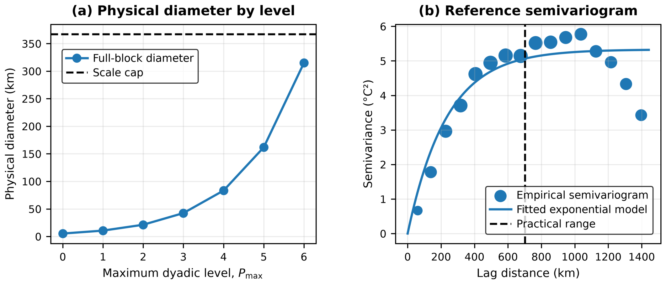
Figure A1 gives the scale diagnostic for M01. The selected
has a representative dyadic side of 13.370 km, while its exact maximum realized WGS84 corner-pair diameter is computed block by block from Equation (
7). The fitted M01 practical range was 701.28 km. The fixed cap is not
times the M01 range alone; it is
times the minimum of the four calibration ranges and equals 366.9376 km. The choice
was fixed before held-out evaluation as a prespecified design margin, not fitted as a coefficient or interpreted as a confidence bound. The maximum realized diameter was 21.157 km on the calibration set and 21.293 km across all twelve temperature fields, so the cap was nonbinding at the selected profile.
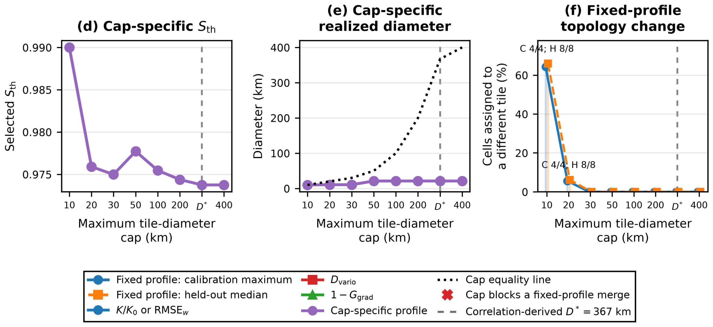
Figure 7 reports the corresponding active-cap sensitivity.
The M01 variogram diagnostic used 110,160 retained sample pairs, a maximum lag of 1442.59 km, and 16 populated bins. The directional practical-range ratio was 5.256, indicating marked directional anisotropy, while the main selection retained the fixed omnidirectional estimate.
Figure A1.
Physical metrics used by the adaptive-grid method. (a) Dyadic physical-scale diagnostics, including exact maximum WGS84 outer-corner diameter, together with the fixed 366.9376 km cap derived from the minimum calibration practical range. (b) M01 empirical semivariogram, pair-count-weighted exponential fit, and fitted practical range. Values provide an M01 reference diagnostic rather than a common range for all fields.
Figure A1.
Physical metrics used by the adaptive-grid method. (a) Dyadic physical-scale diagnostics, including exact maximum WGS84 outer-corner diameter, together with the fixed 366.9376 km cap derived from the minimum calibration practical range. (b) M01 empirical semivariogram, pair-count-weighted exponential fit, and fitted practical range. Values provide an M01 reference diagnostic rather than a common range for all fields.
Appendix C. Alternative Codec Selection Rules
The primary comparison is only one operational question. A common-byte-budget sensitivity first retains candidates whose maximum calibration payload does not exceed the proposed maximum payload. Among these, direct codecs minimize the maximum absolute valid-ocean reconstruction error, whereas hybrids minimize the maximum absolute tile-representative coding error. These are method-specific selection quantities, not a common aggregate of the three plotted fidelity losses. The budget is an upper bound rather than an exact byte match. A second sensitivity builds a method-specific Pareto set in byte ratio and the same three fidelity losses, normalizes within that family, and applies minimax regret. Because normalization bounds differ, regret values cannot be used to rank families.
Table A1 defines every primary and sensitivity operating point, and
Table A2 reports the corresponding calibration maxima on the common byte and fidelity metrics.
The three selection rules answer complementary operational questions. The fidelity-constrained rule asks how small a dense-field codec payload can be while all calibration losses remain within the proposed-profile maxima. The common-budget rule instead asks how much numerical fidelity can be obtained without exceeding the proposed maximum serialized payload. The family-specific minimax rule balances payload and the three losses after normalization within each candidate family. It is therefore a within-family selection device rather than a common score for ranking unlike representations.
Table A1.
Canonical compressor and hybrid operating-point definitions.
Table A1.
Canonical compressor and hybrid operating-point definitions.
| Scenario | Method | Calibration-Selected Parameter |
|---|
| Proposed reference | Proposed adaptive grid | ; ; lossless tile records |
| Primary fidelity-constrained | SZ3 fidelity-constrained | INTERP; ABS = 0.247 |
| Primary fidelity-constrained | ZFP fidelity-constrained | fixed accuracy; requested and effective tolerance = 1 |
| Primary fixed near-fidelity hybrid | AG+SZ3 hybrid | fixed partition + SZ3 LORENZO_REG tile means; ABS = 0.005 |
| Primary fixed near-fidelity hybrid | AG+ZFP hybrid | fixed partition + ZFP-coded tile means; accuracy = 0.005 |
| Common-byte-budget | AG+SZ3 budget-selected | fixed partition + lossless SZ3 tile means |
| Common-byte-budget | AG+ZFP budget-selected | fixed partition + lossless ZFP tile means |
| Common-byte-budget | SZ3 budget-selected | LORENZO_REG; ABS = |
| Common-byte-budget | ZFP budget-selected | fixed accuracy; requested = 0.04, effective = 0.0313 |
| Method-specific four-objective minimax | AG+SZ3 minimax | fixed partition + SZ3 LORENZO_REG tile means; ABS = 0.08 |
| Method-specific four-objective minimax | AG+ZFP minimax | fixed partition + ZFP-coded tile means; accuracy = 0.1 |
| Method-specific four-objective minimax | SZ3 minimax | INTERP; ABS = 0.08 |
| Method-specific four-objective minimax | ZFP minimax | fixed accuracy; requested = 0.32, effective = 0.25 |
Table A2.
Calibration maxima for the reported adaptive-grid, direct-codec, and hybrid operating points.
Table A2.
Calibration maxima for the reported adaptive-grid, direct-codec, and hybrid operating points.
| Method | B | | | |
|---|
| AG+SZ3 budget-selected | 0.2941 | 0.0835 | 0.0078 | 0.1424 |
| AG+SZ3 hybrid | 0.1814 | 0.0836 | 0.0078 | 0.1428 |
| AG+SZ3 minimax | 0.1324 | 0.0955 | 0.0082 | 0.1887 |
| AG+ZFP budget-selected | 0.2903 | 0.0835 | 0.0078 | 0.1424 |
| AG+ZFP hybrid | 0.2080 | 0.0835 | 0.0078 | 0.1425 |
| AG+ZFP minimax | 0.1801 | 0.0842 | 0.0075 | 0.1452 |
| Proposed adaptive grid | 0.3362 | 0.0835 | 0.0078 | 0.1424 |
| SZ3 budget-selected | 0.3352 | 0.0003 | 2.417 × 10⁻⁵ | 0.0009 |
| SZ3 fidelity-constrained | 0.0318 | 0.0834 | 0.0075 | 0.1387 |
| SZ3 minimax | 0.0645 | 0.0312 | 0.0035 | 0.0679 |
| ZFP budget-selected | 0.2965 | 0.0025 | 0.0002 | 0.0069 |
| ZFP fidelity-constrained | 0.1334 | 0.0525 | 0.0064 | 0.1232 |
| ZFP minimax | 0.1869 | 0.0163 | 0.0022 | 0.0424 |
The achieved coordinates in
Table A2 are reported with the rule labels because neither constraint implies exact matching. A budget-selected candidate may leave part of the permitted payload unused, and two fidelity-constrained candidates may distribute their residual loss differently among the three metrics. Moreover, the direct codecs return dense numerical reconstructions, whereas the adaptive and hybrid formats also retain explicit tile geometry and membership. The held-out comparisons below therefore report every achieved coordinate and keep output capability distinct from numerical fidelity.
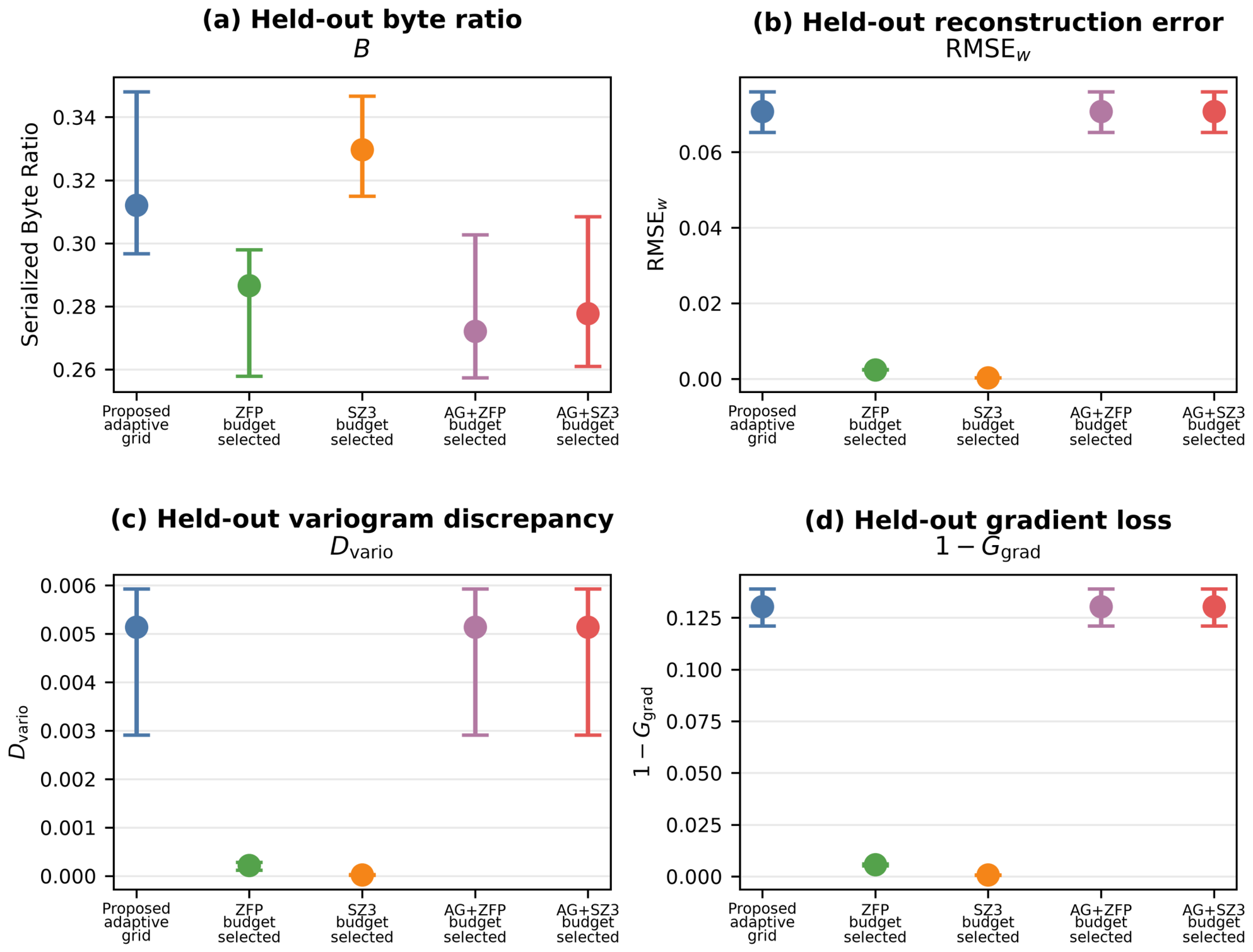
Figure A2 shows that direct-codec settings selected under the calibration payload ceiling retain substantially lower held-out reconstruction losses. For example, the held-out median RMSE was 0.0024 for the budget-selected ZFP point and 0.0003 for the budget-selected SZ3 point. The calibration ceiling does not constrain held-out bytes: the SZ3 setting had a median paired payload increase of 1.1% relative to the proposed representation on held-out fields. The output also lacks the explicit adaptive topology.
Table A3 reports held-out medians for the same operating points, whereas
Table A4 adds field-bootstrap intervals and makes the uncertainty across the sampled held-out fields explicit.
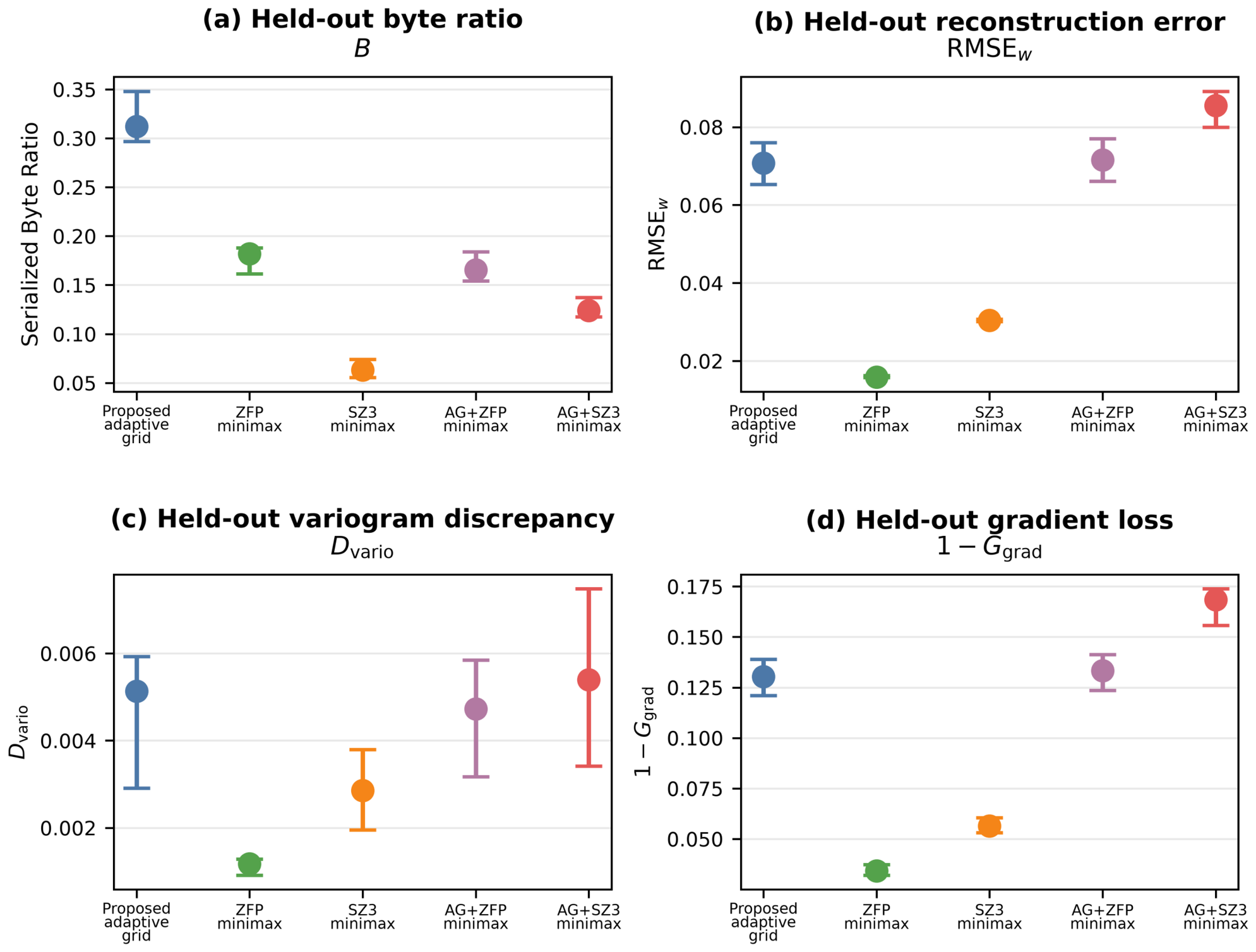
Figure A3 reports family-specific minimax choices. The selected ZFP and SZ3 points have held-out median byte ratios 0.1818 and 0.0630, respectively, with RMSE 0.0159 and 0.0304. Hybrid minimax points save more payload than the primary fixed near-fidelity hybrids but accept larger reconstruction losses, illustrating why the selection question must accompany any reported operating point.
Figure A2.
Held-out sensitivity under a common calibration maximum byte-budget rule. (a) Serialized byte ratio and (b–d) the three fidelity losses. A method may use less than the available budget; held-out byte ratios are not forced to be identical.
Figure A2.
Held-out sensitivity under a common calibration maximum byte-budget rule. (a) Serialized byte ratio and (b–d) the three fidelity losses. A method may use less than the available budget; held-out byte ratios are not forced to be identical.
Table A3.
Held-out medians for all reported adaptive-grid, direct-codec, and hybrid operating points.
Table A3.
Held-out medians for all reported adaptive-grid, direct-codec, and hybrid operating points.
| Method | B | | | |
|---|
| AG+SZ3 budget-selected | 0.2777 | 0.0708 | 0.0051 | 0.1304 |
| AG+SZ3 hybrid | 0.1725 | 0.0709 | 0.0051 | 0.1310 |
| AG+SZ3 minimax | 0.1238 | 0.0855 | 0.0054 | 0.1685 |
| AG+ZFP budget-selected | 0.2721 | 0.0708 | 0.0051 | 0.1304 |
| AG+ZFP hybrid | 0.1907 | 0.0708 | 0.0051 | 0.1305 |
| AG+ZFP minimax | 0.1653 | 0.0715 | 0.0047 | 0.1333 |
| Proposed adaptive grid | 0.3121 | 0.0708 | 0.0051 | 0.1304 |
| SZ3 budget-selected | 0.3297 | 0.0003 | 2.294 × 10⁻⁵ | 0.0007 |
| SZ3 fidelity-constrained | 0.0313 | 0.0815 | 0.0048 | 0.1221 |
| SZ3 minimax | 0.0630 | 0.0304 | 0.0029 | 0.0563 |
| ZFP budget-selected | 0.2867 | 0.0024 | 0.0002 | 0.0056 |
| ZFP fidelity-constrained | 0.1284 | 0.0508 | 0.0034 | 0.1018 |
| ZFP minimax | 0.1818 | 0.0159 | 0.0012 | 0.0342 |
Figure A3.
Held-out sensitivity for method-specific four-objective minimax selection. Each family is normalized using its own calibration Pareto extrema. The panel therefore compares the resulting operating points, not the family-specific normalized regret values themselves.
Figure A3.
Held-out sensitivity for method-specific four-objective minimax selection. Each family is normalized using its own calibration Pareto extrema. The panel therefore compares the resulting operating points, not the family-specific normalized regret values themselves.
Table A4.
Held-out medians and 95% field-bootstrap intervals for all reported operating points (5000 resamples). Each metric entry is the median [2.5th, 97.5th percentile].
Table A4.
Held-out medians and 95% field-bootstrap intervals for all reported operating points (5000 resamples). Each metric entry is the median [2.5th, 97.5th percentile].
| Method | B | | | |
|---|
| AG+SZ3 budget-selected | 0.2777 [0.2611, 0.3085] | 0.0708 [0.0653, 0.0760] | 0.0051 [0.0029, 0.0059] | 0.1304 [0.1210, 0.1389] |
| AG+SZ3 hybrid | 0.1725 [0.1609, 0.1862] | 0.0709 [0.0653, 0.0764] | 0.0051 [0.0032, 0.0059] | 0.1310 [0.1214, 0.1384] |
| AG+SZ3 minimax | 0.1238 [0.1173, 0.1373] | 0.0855 [0.0800, 0.0892] | 0.0054 [0.0034, 0.0075] | 0.1685 [0.1557, 0.1739] |
| AG+ZFP budget-selected | 0.2721 [0.2574, 0.3027] | 0.0708 [0.0653, 0.0760] | 0.0051 [0.0029, 0.0059] | 0.1304 [0.1210, 0.1389] |
| AG+ZFP hybrid | 0.1907 [0.1788, 0.2126] | 0.0708 [0.0653, 0.0763] | 0.0051 [0.0029, 0.0059] | 0.1305 [0.1210, 0.1390] |
| AG+ZFP minimax | 0.1653 [0.1543, 0.1839] | 0.0715 [0.0661, 0.0770] | 0.0047 [0.0032, 0.0059] | 0.1333 [0.1235, 0.1413] |
| Proposed adaptive grid | 0.3121 [0.2968, 0.3481] | 0.0708 [0.0653, 0.0760] | 0.0051 [0.0029, 0.0059] | 0.1304 [0.1210, 0.1389] |
| SZ3 budget-selected | 0.3297 [0.3150, 0.3467] | 0.0003 [0.0003, 0.0003] | 2.294 × 10⁻⁵ [1.628 × 10⁻⁵, 2.743 × 10⁻⁵] | 0.0007 [0.0006, 0.0008] |
| SZ3 fidelity-constrained | 0.0313 [0.0257, 0.0383] | 0.0815 [0.0797, 0.0820] | 0.0048 [0.0034, 0.0086] | 0.1221 [0.1150, 0.1286] |
| SZ3 minimax | 0.0630 [0.0555, 0.0741] | 0.0304 [0.0301, 0.0307] | 0.0029 [0.0020, 0.0038] | 0.0563 [0.0531, 0.0605] |
| ZFP budget-selected | 0.2867 [0.2579, 0.2979] | 0.0024 [0.0024, 0.0025] | 0.0002 [0.0001, 0.0003] | 0.0056 [0.0051, 0.0060] |
| ZFP fidelity-constrained | 0.1284 [0.1139, 0.1347] | 0.0508 [0.0501, 0.0514] | 0.0034 [0.0022, 0.0044] | 0.1018 [0.0971, 0.1105] |
| ZFP minimax | 0.1818 [0.1615, 0.1881] | 0.0159 [0.0158, 0.0163] | 0.0012 [0.0009, 0.0013] | 0.0342 [0.0321, 0.0373] |
Appendix D. Harmonized Runtime Protocol
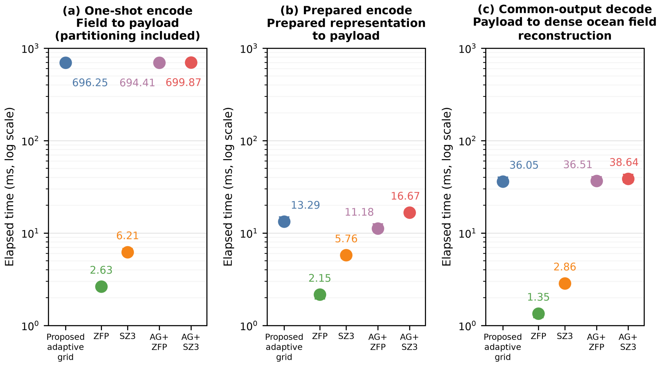
Figure A4 reports the three timing boundaries defined in
Section 2. The field-level medians were bootstrapped over the same eight held-out fields. One-shot adaptive timings include construction of the partition; prepared-representation timings remove that construction and expose serialization of an already prepared representation. Common-output decoding requires every method to return a dense float32 ocean reconstruction.
Figure A4.
Harmonized implementation timing diagnostic. (a) One-shot field-to-payload encoding. (b) Prepared-representation-to-payload encoding. (c) Payload-to-dense-float32 common-output decoding. Points are held-out medians and bars are field-bootstrap intervals. NetCDF I/O, calibration, and fidelity metrics are excluded; compiled codec paths and Python adaptive paths prevent a language-neutral speed ranking.
Figure A4.
Harmonized implementation timing diagnostic. (a) One-shot field-to-payload encoding. (b) Prepared-representation-to-payload encoding. (c) Payload-to-dense-float32 common-output decoding. Points are held-out medians and bars are field-bootstrap intervals. NetCDF I/O, calibration, and fidelity metrics are excluded; compiled codec paths and Python adaptive paths prevent a language-neutral speed ranking.
Appendix E. Hybrid Operating-Space Analysis
Table A5 and
Table A6 report field-level metrics and held-out changes for the primary operating points. All reported byte ratios use the common denominator and measured wrapper rules defined in the Methods. The adaptive and hybrid records preserve the same tile geometry and membership scope but use their respective serialization layouts, whereas the direct codecs contain dense coded values and no adaptive-topology record.
The field-level rows separate effects of the fixed partition from effects of representative-value coding. Within each hybrid family, tile geometry, membership, and tile count are identical to the proposed representation; changes in payload arise from coding the representative-value stream, and changes in fidelity appear after those values are decoded and expanded to the dense ocean grid. Direct ZFP and SZ3 operate on the dense field and therefore do not share this fixed-topology interpretation.
Table A6 expresses medians of field-paired percentage changes relative to the proposed representation, rather than percentage changes between separately aggregated medians. Because all four reported quantities are minimized, a negative percentage denotes a reduction in payload or loss and a positive percentage denotes an increase. The signs are deliberately not collapsed into a single score: a smaller payload can accompany either smaller or larger fidelity losses, and the appropriate trade-off depends on the selection rule and the required output capability.
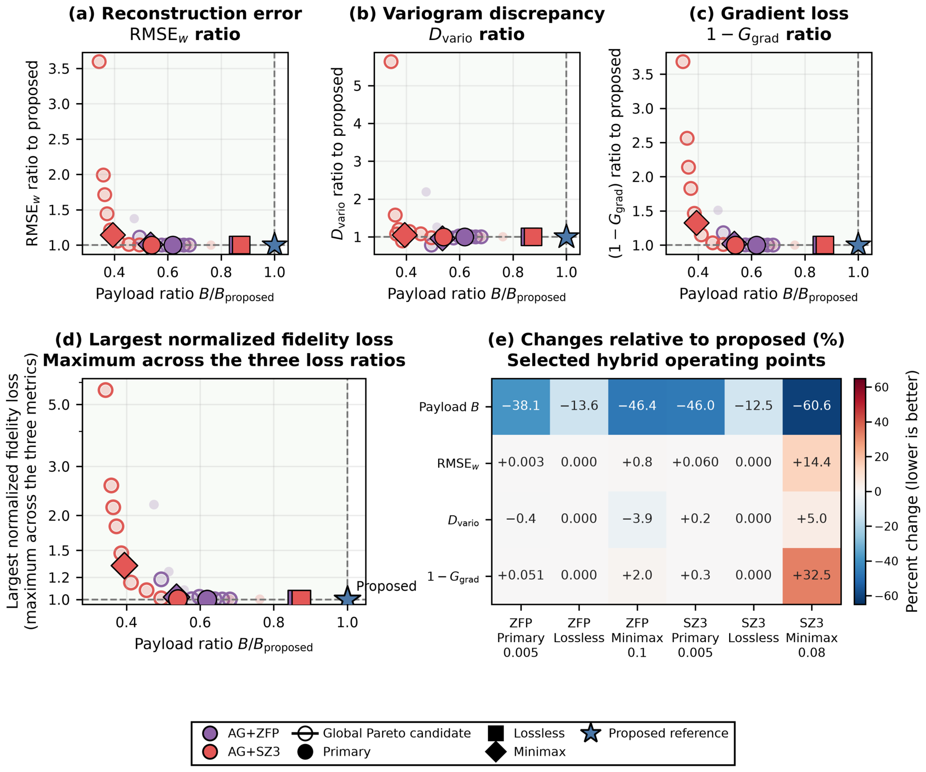
Figure A5 shows candidate projections after applying ZFP or SZ3 to tile representatives under a fixed adaptive partition. The primary choices keep calibration fidelity ratios close to the unhybridized adaptive reference, while the wider candidate sets expose the payload–fidelity alternatives available when representative values alone are coded.
Table A5.
Field-level metrics for the five primary methods. Cal. denotes calibration; the complete 156-row machine-readable CSV file includes alternative selection scenarios.
Table A5.
Field-level metrics for the five primary methods. Cal. denotes calibration; the complete 156-row machine-readable CSV file includes alternative selection scenarios.
| Field | Role | B | | | |
|---|
| Proposed adaptive grid |
| M01 | Cal. | 0.3236 | 0.0835 | 0.0066 | 0.1291 |
| M02 | Held-out | 0.3069 | 0.0758 | 0.0037 | 0.1319 |
| M03 | Held-out | 0.3020 | 0.0717 | 0.0054 | 0.1289 |
| M04 | Cal. | 0.2949 | 0.0686 | 0.0032 | 0.1424 |
| M05 | Held-out | 0.2944 | 0.0653 | 0.0049 | 0.1437 |
| M06 | Held-out | 0.3173 | 0.0699 | 0.0056 | 0.1320 |
| M07 | Cal. | 0.3362 | 0.0708 | 0.0078 | 0.1274 |
| M08 | Held-out | 0.3894 | 0.0637 | 0.0059 | 0.0942 |
| M09 | Held-out | 0.2968 | 0.0774 | 0.0029 | 0.1389 |
| M10 | Cal. | 0.3146 | 0.0625 | 0.0032 | 0.1369 |
| M11 | Held-out | 0.3402 | 0.0668 | 0.0102 | 0.1250 |
| M12 | Held-out | 0.3481 | 0.0763 | 0.0028 | 0.1210 |
| ZFP fidelity-constrained |
| M01 | Cal. | 0.1191 | 0.0525 | 0.0029 | 0.0921 |
| M02 | Held-out | 0.1139 | 0.0507 | 0.0032 | 0.0991 |
| M03 | Held-out | 0.1110 | 0.0489 | 0.0022 | 0.1017 |
| M04 | Cal. | 0.1089 | 0.0492 | 0.0035 | 0.1148 |
| M05 | Held-out | 0.1216 | 0.0501 | 0.0021 | 0.1217 |
| M06 | Held-out | 0.1336 | 0.0511 | 0.0041 | 0.1068 |
| M07 | Cal. | 0.1334 | 0.0510 | 0.0028 | 0.1030 |
| M08 | Held-out | 0.1402 | 0.0514 | 0.0053 | 0.0891 |
| M09 | Held-out | 0.1347 | 0.0510 | 0.0037 | 0.1019 |
| M10 | Cal. | 0.1243 | 0.0489 | 0.0064 | 0.1232 |
| M11 | Held-out | 0.1268 | 0.0506 | 0.0044 | 0.1105 |
| M12 | Held-out | 0.1299 | 0.0531 | 0.0026 | 0.0971 |
| SZ3 fidelity-constrained |
| M01 | Cal. | 0.0311 | 0.0834 | 0.0041 | 0.1112 |
| M02 | Held-out | 0.0277 | 0.0819 | 0.0049 | 0.1195 |
| M03 | Held-out | 0.0245 | 0.0797 | 0.0086 | 0.1247 |
| M04 | Cal. | 0.0242 | 0.0793 | 0.0075 | 0.1292 |
| M05 | Held-out | 0.0308 | 0.0793 | 0.0058 | 0.1378 |
| M06 | Held-out | 0.0383 | 0.0820 | 0.0033 | 0.1251 |
| M07 | Cal. | 0.0318 | 0.0809 | 0.0023 | 0.1182 |
| M08 | Held-out | 0.0388 | 0.0818 | 0.0047 | 0.1015 |
| M09 | Held-out | 0.0319 | 0.0812 | 0.0034 | 0.1150 |
| M10 | Cal. | 0.0207 | 0.0795 | 0.0046 | 0.1387 |
| M11 | Held-out | 0.0257 | 0.0805 | 0.0092 | 0.1286 |
| M12 | Held-out | 0.0380 | 0.0842 | 0.0041 | 0.1167 |
| AG+ZFP hybrid |
| M01 | Cal. | 0.1940 | 0.0835 | 0.0066 | 0.1291 |
| M02 | Held-out | 0.1825 | 0.0758 | 0.0038 | 0.1320 |
| M03 | Held-out | 0.1788 | 0.0717 | 0.0054 | 0.1290 |
| M04 | Cal. | 0.1753 | 0.0686 | 0.0031 | 0.1425 |
| M05 | Held-out | 0.1781 | 0.0653 | 0.0049 | 0.1437 |
| M06 | Held-out | 0.1946 | 0.0699 | 0.0056 | 0.1321 |
| M07 | Cal. | 0.2080 | 0.0708 | 0.0078 | 0.1275 |
| M08 | Held-out | 0.2423 | 0.0637 | 0.0059 | 0.0944 |
| M09 | Held-out | 0.1869 | 0.0774 | 0.0029 | 0.1390 |
| M10 | Cal. | 0.1967 | 0.0625 | 0.0032 | 0.1369 |
| M11 | Held-out | 0.2106 | 0.0668 | 0.0103 | 0.1251 |
| M12 | Held-out | 0.2126 | 0.0763 | 0.0028 | 0.1210 |
| AG+SZ3 hybrid |
| M01 | Cal. | 0.1778 | 0.0836 | 0.0066 | 0.1295 |
| M02 | Held-out | 0.1691 | 0.0758 | 0.0036 | 0.1324 |
| M03 | Held-out | 0.1609 | 0.0717 | 0.0057 | 0.1296 |
| M04 | Cal. | 0.1588 | 0.0687 | 0.0031 | 0.1428 |
| M05 | Held-out | 0.1606 | 0.0653 | 0.0047 | 0.1442 |
| M06 | Held-out | 0.1743 | 0.0700 | 0.0055 | 0.1326 |
| M07 | Cal. | 0.1814 | 0.0708 | 0.0078 | 0.1280 |
| M08 | Held-out | 0.2083 | 0.0638 | 0.0059 | 0.0949 |
| M09 | Held-out | 0.1707 | 0.0775 | 0.0031 | 0.1394 |
| M10 | Cal. | 0.1684 | 0.0626 | 0.0034 | 0.1373 |
| M11 | Held-out | 0.1790 | 0.0668 | 0.0101 | 0.1255 |
| M12 | Held-out | 0.1862 | 0.0764 | 0.0028 | 0.1214 |
Figure A5.
Hybrid operating-space analysis. (a–c) Normalized payload–loss projections for candidate AG+ZFP and AG+SZ3 tile-value settings. (d) Largest normalized fidelity loss. (e) Percentage changes at selected points. The partition, geometry, and membership remain fixed; only representative tile values are coded.
Figure A5.
Hybrid operating-space analysis. (a–c) Normalized payload–loss projections for candidate AG+ZFP and AG+SZ3 tile-value settings. (d) Largest normalized fidelity loss. (e) Percentage changes at selected points. The partition, geometry, and membership remain fixed; only representative tile values are coded.
Table A6.
Medians of held-out field-paired percentage changes relative to the proposed adaptive grid. Ratios are formed within each field before aggregation. All four numeric columns report percentages; negative values denote reductions.
Table A6.
Medians of held-out field-paired percentage changes relative to the proposed adaptive grid. Ratios are formed within each field before aggregation. All four numeric columns report percentages; negative values denote reductions.
| Method/Scenario | | | | |
|---|
| AG+SZ3 budget-selected (Common-byte-budget) | −11.44 | 0 | 0 | 0 |
| AG+SZ3 hybrid (Primary fixed near-fidelity hybrid) | −45.98 | 0.08 | −0.47 | 0.40 |
| AG+SZ3 minimax (Method-specific four-objective minimax) | −60.52 | 20.75 | 21.48 | 30.00 |
| AG+ZFP budget-selected (Common-byte-budget) | −13.13 | 0 | 0 | 0 |
| AG+ZFP hybrid (Primary fixed near-fidelity hybrid) | −38.81 | 0.00 | 0.12 | 0.06 |
| AG+ZFP minimax (Method-specific four-objective minimax) | −47.04 | 1.05 | −3.46 | 2.16 |
| SZ3 budget-selected (Common-byte-budget) | 1.11 | −99.55 | −99.57 | −99.42 |
| SZ3 fidelity-constrained (Primary fidelity-constrained) | −89.79 | 14.23 | 17.23 | −3.84 |
| SZ3 minimax (Method-specific four-objective minimax) | −79.89 | −57.26 | −44.90 | −55.48 |
| ZFP budget-selected (Common-byte-budget) | −15.98 | −96.56 | −96.26 | −95.49 |
| ZFP fidelity-constrained (Primary fidelity-constrained) | −62.70 | −28.67 | −21.40 | −19.39 |
| ZFP minimax (Method-specific four-objective minimax) | −47.08 | −77.59 | −76.16 | −72.78 |
Figure 1.
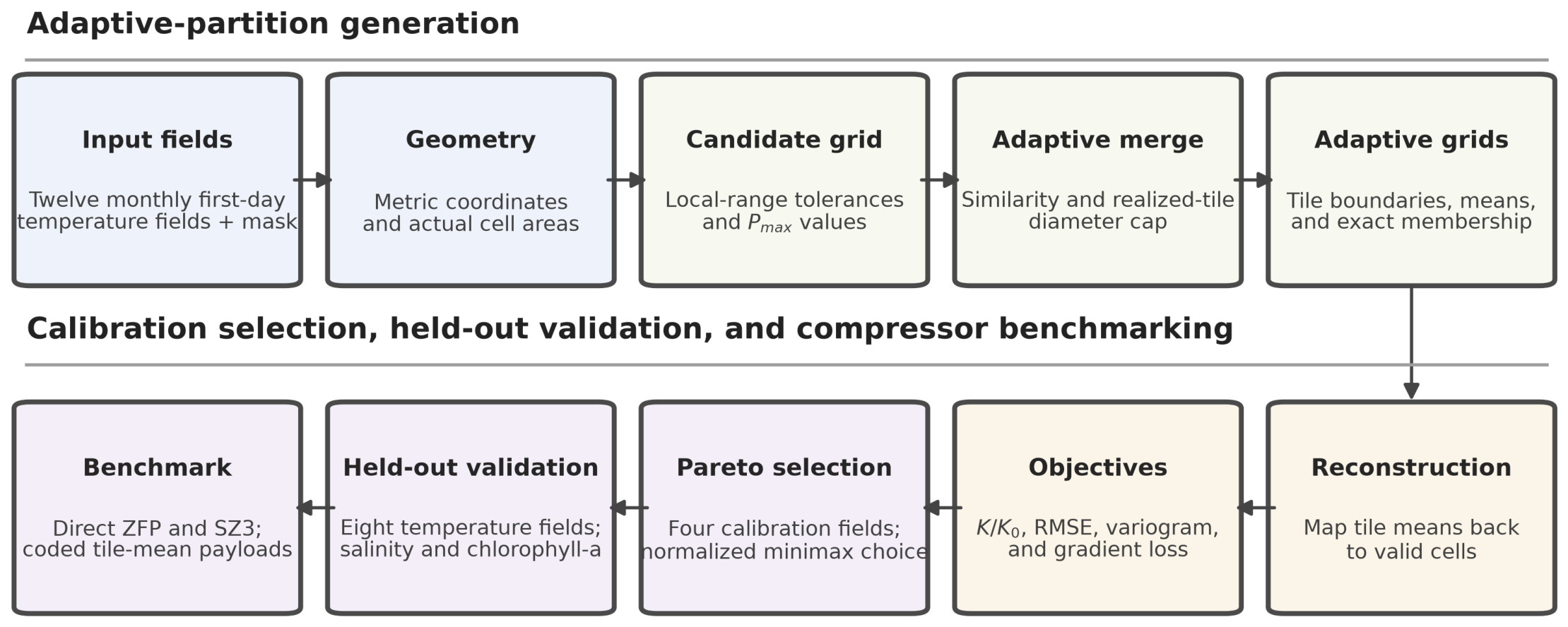
Analysis workflow and pipeline. Four calibration fields determine one adaptive parameter profile by exact realized-tile scale screening, Pareto filtering, and normalized minimax regret. The profile is fixed before field-specific partitions are regenerated for eight within-sequence held-out fields. Same-grid salinity, external satellite chlorophyll-a, spatial comparators, direct codecs, hybrids, and runtime protocols are evaluated in distinct branches. The output is a lossy derived field with an explicit partition and exact tile-to-cell membership rather than a replacement numerical-model grid.
Figure 1.
Analysis workflow and pipeline. Four calibration fields determine one adaptive parameter profile by exact realized-tile scale screening, Pareto filtering, and normalized minimax regret. The profile is fixed before field-specific partitions are regenerated for eight within-sequence held-out fields. Same-grid salinity, external satellite chlorophyll-a, spatial comparators, direct codecs, hybrids, and runtime protocols are evaluated in distinct branches. The output is a lossy derived field with an explicit partition and exact tile-to-cell membership rather than a replacement numerical-model grid.
Figure 2.
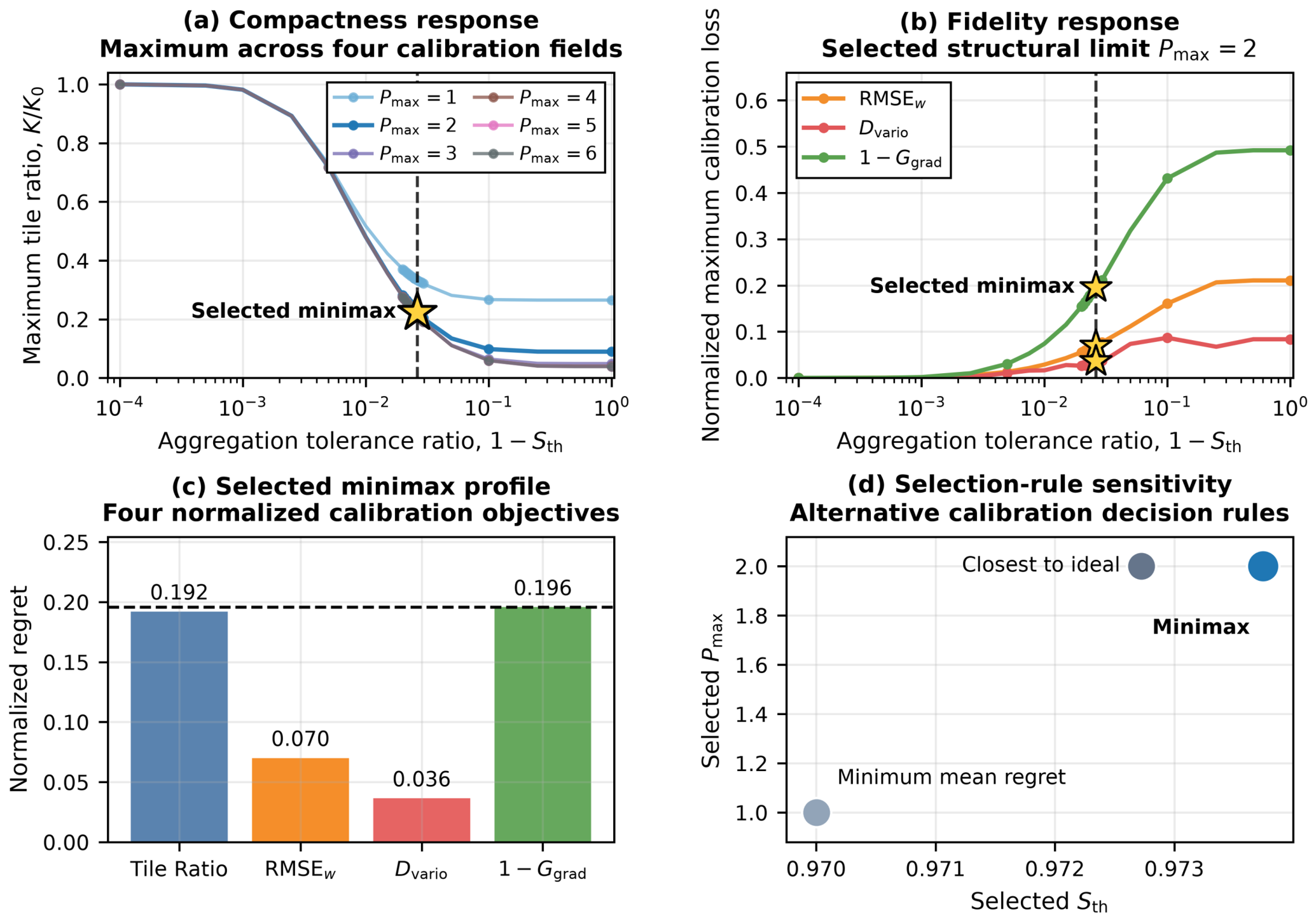
Parameter response and fixed-profile selection. (a) Structural tile ratio as a function of the aggregation-tolerance ratio across maximum dyadic levels. The singleton case is omitted, and and 8 coincide with throughout the displayed strict complete-block search, so only levels 1–6 are shown. (b) Normalized fidelity responses at the selected . (c) Four normalized objective regrets of the selected calibration point. (d) Sensitivity of the selected operating point to alternative calibration-only decision rules. The star denotes and , and the vertical dashed lines in (a,b) mark its horizontal-axis position; the held-out fields are not used in any panel. The horizontal dashed line in (c) marks the maximum normalized regret of the selected point.
Figure 2.
Parameter response and fixed-profile selection. (a) Structural tile ratio as a function of the aggregation-tolerance ratio across maximum dyadic levels. The singleton case is omitted, and and 8 coincide with throughout the displayed strict complete-block search, so only levels 1–6 are shown. (b) Normalized fidelity responses at the selected . (c) Four normalized objective regrets of the selected calibration point. (d) Sensitivity of the selected operating point to alternative calibration-only decision rules. The star denotes and , and the vertical dashed lines in (a,b) mark its horizontal-axis position; the held-out fields are not used in any panel. The horizontal dashed line in (c) marks the maximum normalized regret of the selected point.
Figure 3.
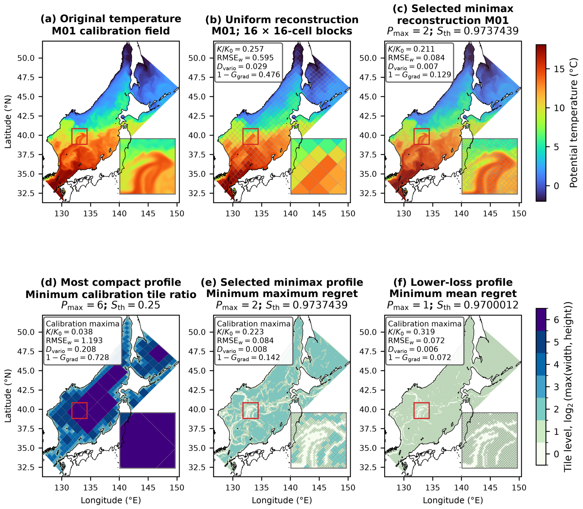
Spatial consequences of candidate selection. (a) Original M01 field. (b) Nearest discrete uniform representation for M01. (c) Selected minimax reconstruction for M01. (d) Compactness-prioritized calibration state. (e) Tile-level map of the selected calibration profile. (f) Candidate selected by minimum mean regret, which favors lower losses. Insets use a common narrower region to expose tile boundaries and local reconstruction behavior. Panels (b,c) report M01 values; panels (d–f) identify states using maxima over M01, M04, M07, and M10.
Figure 3.
Spatial consequences of candidate selection. (a) Original M01 field. (b) Nearest discrete uniform representation for M01. (c) Selected minimax reconstruction for M01. (d) Compactness-prioritized calibration state. (e) Tile-level map of the selected calibration profile. (f) Candidate selected by minimum mean regret, which favors lower losses. Insets use a common narrower region to expose tile boundaries and local reconstruction behavior. Panels (b,c) report M01 values; panels (d–f) identify states using maxima over M01, M04, M07, and M10.
Figure 4.
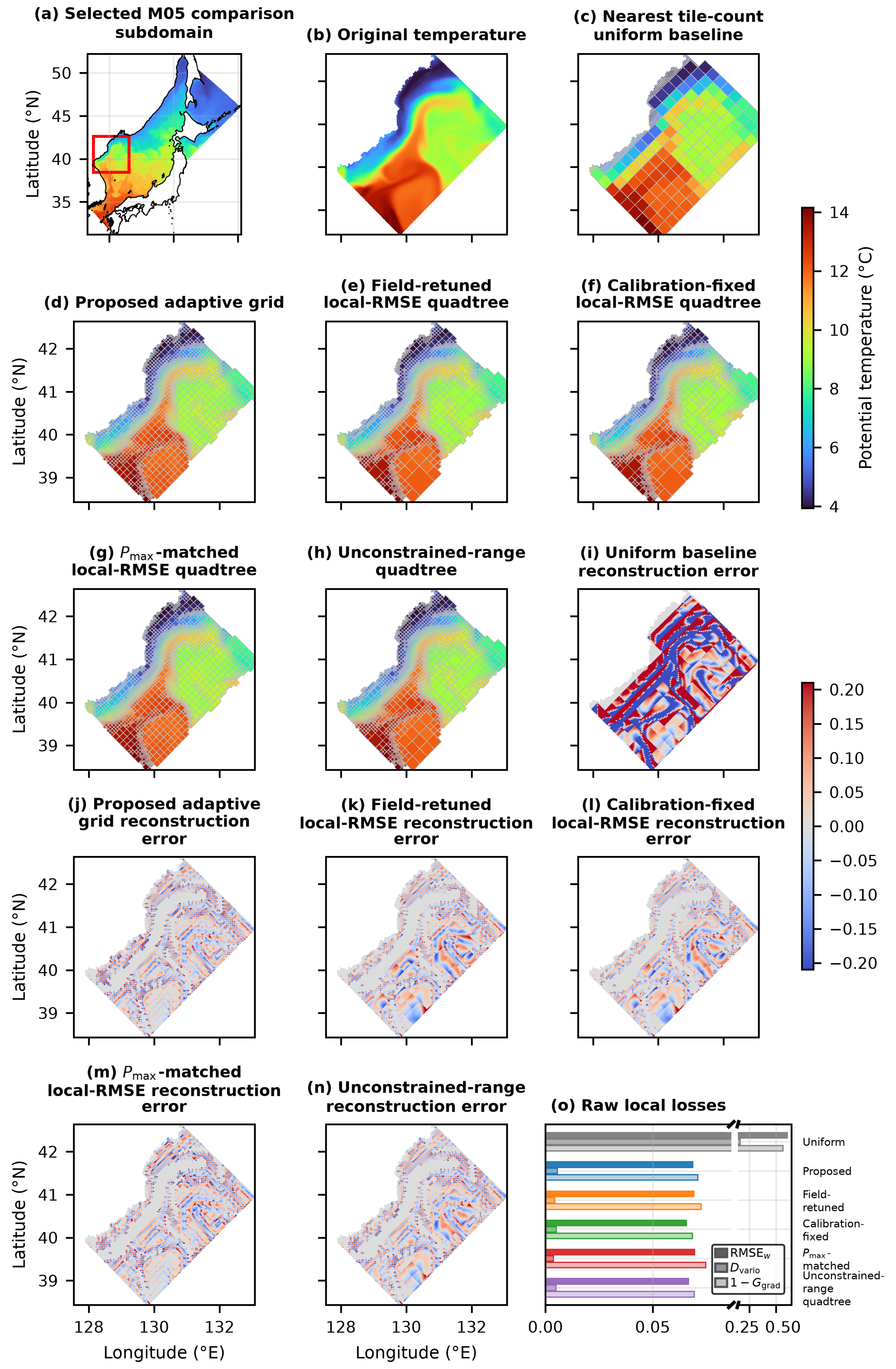
Spatial comparison on M05. (a) Comparison subdomain; (b) original field; (c) uniform representation; (d) proposed adaptive grid; and (e–h) quadtree representations. (i–n) Reconstruction errors on a common color scale. (o) Raw local RMSE, semivariogram discrepancy, and gradient-magnitude loss. M05 is held out, and the displayed subdomain is diagnostic only.
Figure 4.
Spatial comparison on M05. (a) Comparison subdomain; (b) original field; (c) uniform representation; (d) proposed adaptive grid; and (e–h) quadtree representations. (i–n) Reconstruction errors on a common color scale. (o) Raw local RMSE, semivariogram discrepancy, and gradient-magnitude loss. M05 is held out, and the displayed subdomain is diagnostic only.
Figure 5.
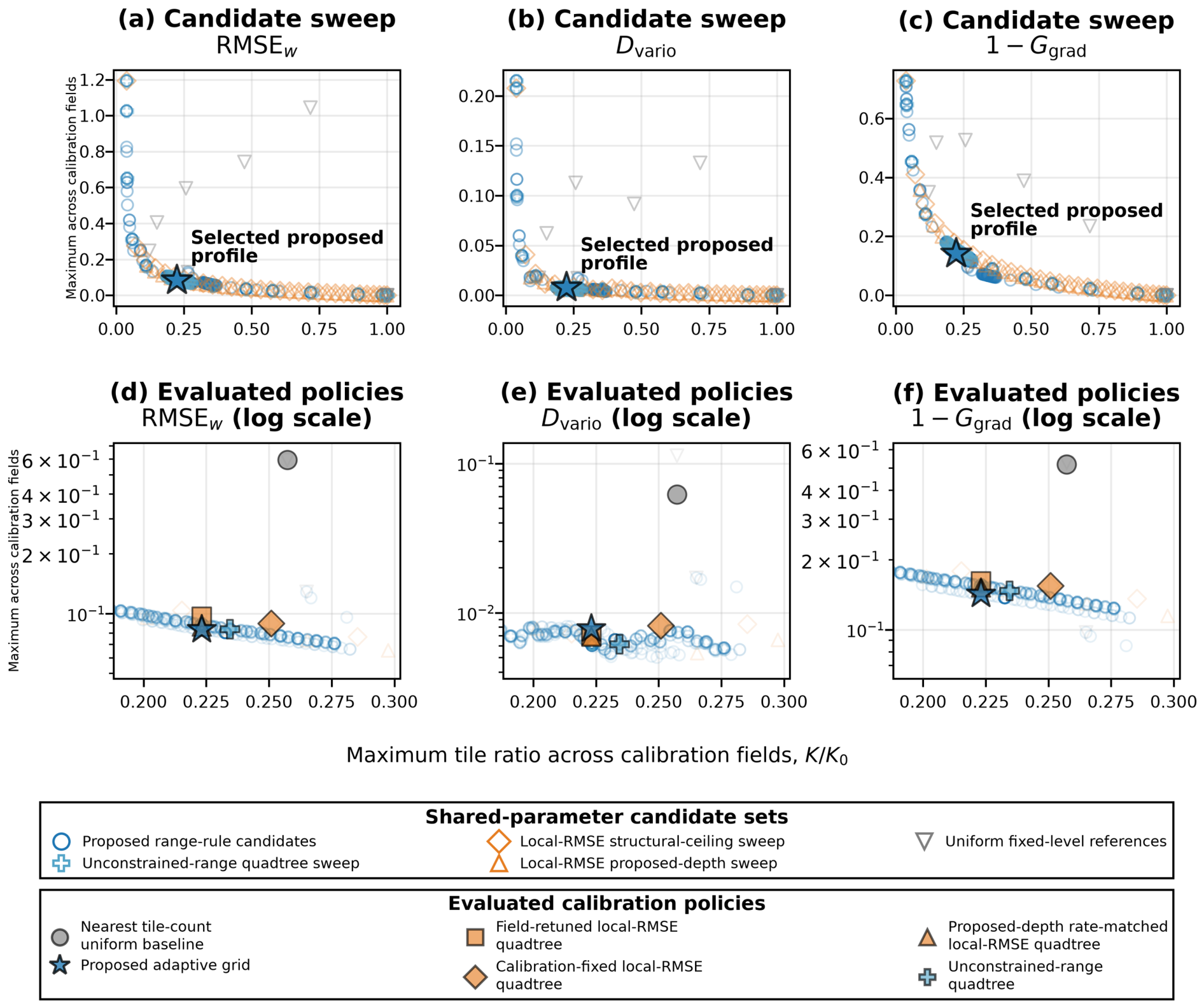
Calibration candidate sets and evaluated policies. Columns compare the maximum tile ratio across the four calibration fields with maximum (
a,
d)
, (
b,
e)
, and (
c,
f)
. Lower-left locations are preferable within each panel because both structural burden and fidelity loss are smaller. Open markers in the upper row show shared-parameter candidate sweeps. In the lower row, translucent filled markers identify the five comparators, whereas the black-outlined blue star highlights the proposed four-objective minimax profile. Blue denotes range-rule constructions, orange denotes local-RMSE constructions, and gray denotes uniform references. The Field-retuned and proposed-depth rate-matched local-RMSE policies use field-specific tolerances and therefore appear as evaluated points rather than shared-parameter calibration curves. The unconstrained-range policy is the Unconstrained-range comparator in
Table 2. The lower-row loss axes use logarithmic scaling to keep all evaluated policies legible.
Figure 5.
Calibration candidate sets and evaluated policies. Columns compare the maximum tile ratio across the four calibration fields with maximum (
a,
d)
, (
b,
e)
, and (
c,
f)
. Lower-left locations are preferable within each panel because both structural burden and fidelity loss are smaller. Open markers in the upper row show shared-parameter candidate sweeps. In the lower row, translucent filled markers identify the five comparators, whereas the black-outlined blue star highlights the proposed four-objective minimax profile. Blue denotes range-rule constructions, orange denotes local-RMSE constructions, and gray denotes uniform references. The Field-retuned and proposed-depth rate-matched local-RMSE policies use field-specific tolerances and therefore appear as evaluated points rather than shared-parameter calibration curves. The unconstrained-range policy is the Unconstrained-range comparator in
Table 2. The lower-row loss axes use logarithmic scaling to keep all evaluated policies legible.

Figure 6.
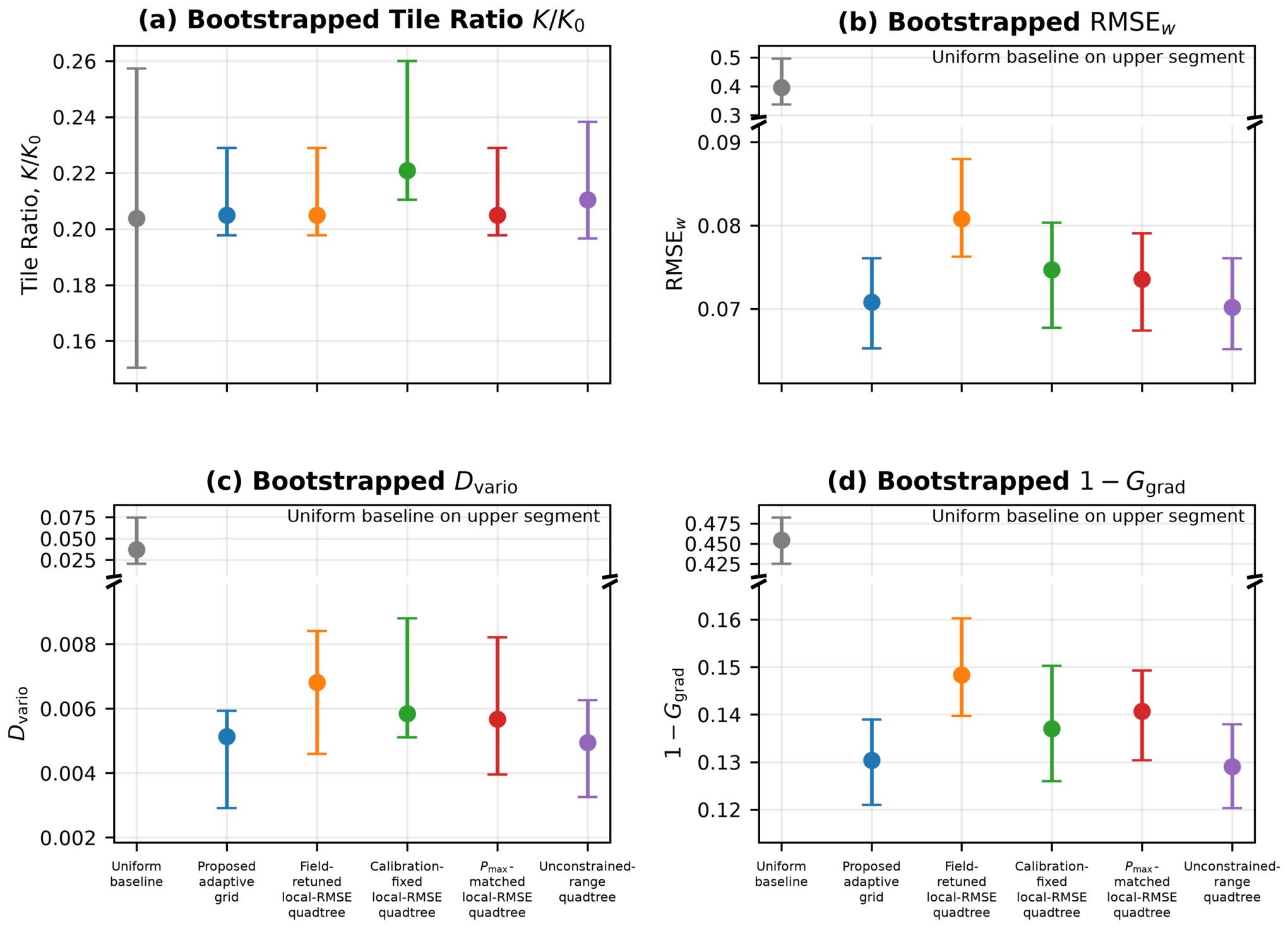
East Sea within-sequence held-out performance of the six spatial methods. Points are medians across the eight noncalibration nominal monthly first-day fields; bars are 2.5th–97.5th percentiles from 5000 field-level bootstrap resamples. (a) Structural tile ratio . (b) Area-weighted RMSE. (c) Normalized semivariogram discrepancy. (d) Physical-gradient magnitude loss. A partition is regenerated from each field. Broken axes enlarge the adaptive-method region where the uniform result is much larger.
Figure 6.
East Sea within-sequence held-out performance of the six spatial methods. Points are medians across the eight noncalibration nominal monthly first-day fields; bars are 2.5th–97.5th percentiles from 5000 field-level bootstrap resamples. (a) Structural tile ratio . (b) Area-weighted RMSE. (c) Normalized semivariogram discrepancy. (d) Physical-gradient magnitude loss. A partition is regenerated from each field. Broken axes enlarge the adaptive-method region where the uniform result is much larger.
Figure 7.
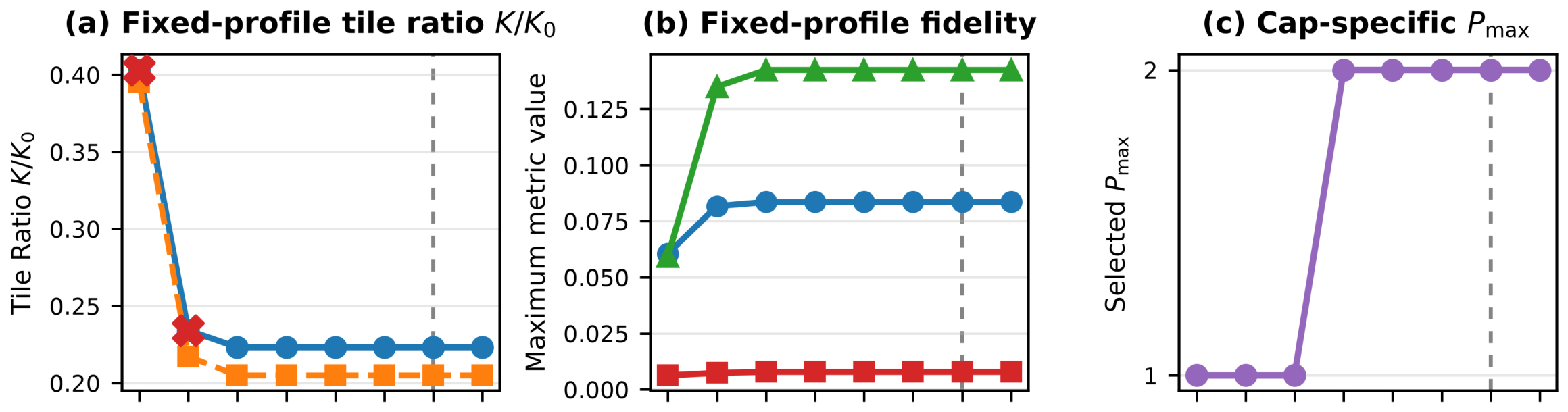
Exact realized-tile scale-cap sensitivity under two explicitly separated analysis protocols. Panels (a,b,f) apply the fixed calibration-selected temperature profile at every cap: (a) calibration-maximum and held-out-median tile ratios; (b) calibration-maximum fidelity losses; and (f) the median fraction of valid cells whose containing tile differs from the uncapped fixed-profile partition, shown separately for calibration and held-out fields. This fixed profile binds in 4/4 calibration and 8/8 held-out fields at 10 and 20 km, and in 0 fields at caps of 30 km or greater. Panels (c–e) use cap-specific calibration: (c) selected , (d) selected , and (e) maximum realized tile diameter. Only the 10 km cap-specific profile binds (4/4 calibration and 8/8 held-out fields). The vertical dashed line marks the 366.9376 km correlation-derived cap. Tile diameter is the maximum WGS84 geodesic distance among the six pairs of outer block corners.
Figure 7.
Exact realized-tile scale-cap sensitivity under two explicitly separated analysis protocols. Panels (a,b,f) apply the fixed calibration-selected temperature profile at every cap: (a) calibration-maximum and held-out-median tile ratios; (b) calibration-maximum fidelity losses; and (f) the median fraction of valid cells whose containing tile differs from the uncapped fixed-profile partition, shown separately for calibration and held-out fields. This fixed profile binds in 4/4 calibration and 8/8 held-out fields at 10 and 20 km, and in 0 fields at caps of 30 km or greater. Panels (c–e) use cap-specific calibration: (c) selected , (d) selected , and (e) maximum realized tile diameter. Only the 10 km cap-specific profile binds (4/4 calibration and 8/8 held-out fields). The vertical dashed line marks the 366.9376 km correlation-derived cap. Tile diameter is the maximum WGS84 geodesic distance among the six pairs of outer block corners.
Figure 8.
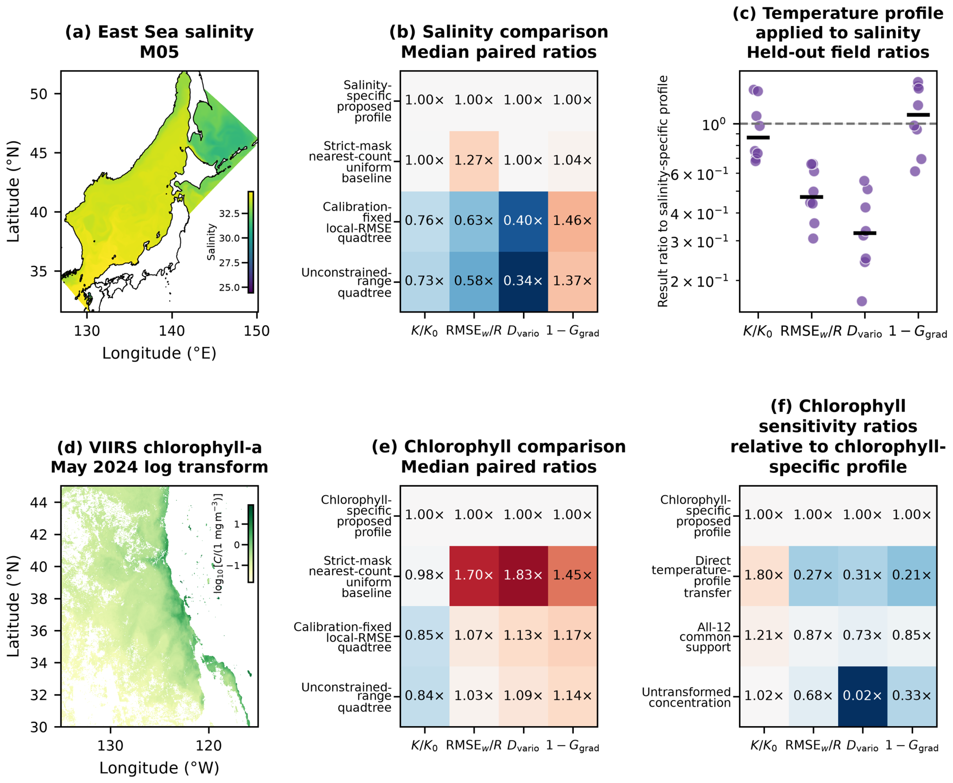
Cross-variable and external-observation validation. (a) East Sea M05 near-surface salinity. (b) Median field-paired held-out salinity ratios relative to the salinity-specific proposed profile for structural tile ratio, normalized RMSE, normalized semivariogram discrepancy, and physical-gradient magnitude loss. (c) Field-level ratios obtained by direct temperature-profile transfer to salinity without recalibration. (d) California Current NOAA VIIRS chlorophyll-a for May 2024, displayed and analyzed primarily as the dimensionless field . (e) Median field-paired held-out VIIRS ratios relative to the chlorophyll-specific proposed profile. (f) Chlorophyll support, transform, and direct-transfer sensitivities. Relative summaries are formed within each field before aggregation. Raw-concentration versus log-transformed ratios in (f) describe transform sensitivity rather than errors on a common physical scale. The scale screen was nonbinding in these case studies. In (b,e,f), blue and red indicate ratios below and above 1, respectively, with white centered at 1; color intensity follows a panel-specific ratio scale. In (c), purple dots show individual held-out field ratios, black horizontal bars show their medians, and the dashed line marks a ratio of 1.
Figure 8.
Cross-variable and external-observation validation. (a) East Sea M05 near-surface salinity. (b) Median field-paired held-out salinity ratios relative to the salinity-specific proposed profile for structural tile ratio, normalized RMSE, normalized semivariogram discrepancy, and physical-gradient magnitude loss. (c) Field-level ratios obtained by direct temperature-profile transfer to salinity without recalibration. (d) California Current NOAA VIIRS chlorophyll-a for May 2024, displayed and analyzed primarily as the dimensionless field . (e) Median field-paired held-out VIIRS ratios relative to the chlorophyll-specific proposed profile. (f) Chlorophyll support, transform, and direct-transfer sensitivities. Relative summaries are formed within each field before aggregation. Raw-concentration versus log-transformed ratios in (f) describe transform sensitivity rather than errors on a common physical scale. The scale screen was nonbinding in these case studies. In (b,e,f), blue and red indicate ratios below and above 1, respectively, with white centered at 1; color intensity follows a panel-specific ratio scale. In (c), purple dots show individual held-out field ratios, black horizontal bars show their medians, and the dashed line marks a ratio of 1.

Figure 9.
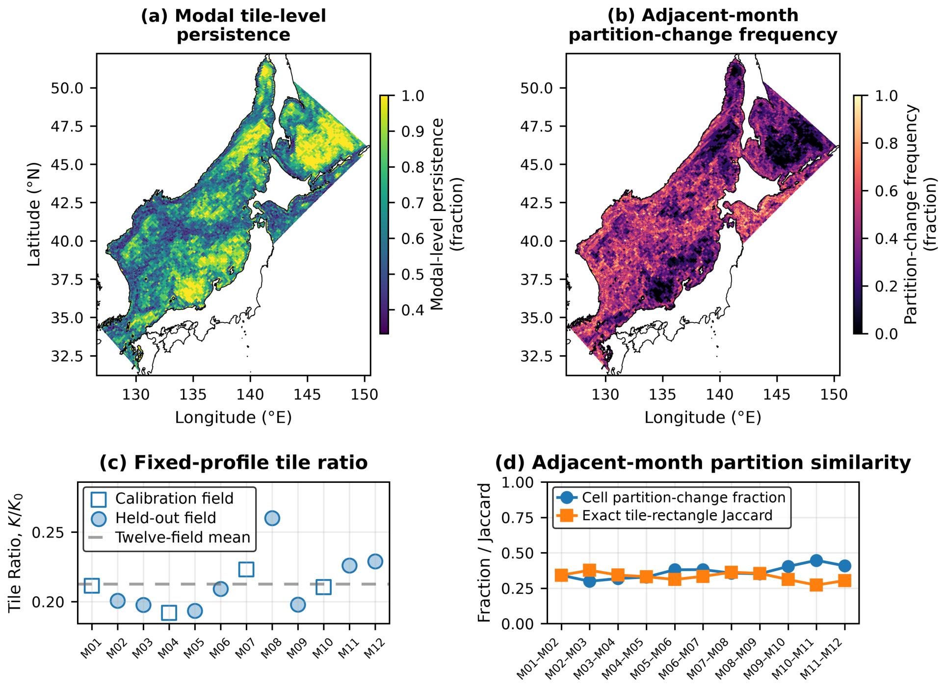
Monthly first-day adaptive-partition topology diagnostic. (a) Persistence of each cell’s modal tile level. (b) Frequency with which the exact containing tile rectangle changes across 11 adjacent monthly first-day pairs. (c) Monthly tile ratio; the translucent gray dashed line is the twelve-field mean. (d) Adjacent-pair cell partition-change fraction and exact tile-rectangle Jaccard similarity. Similar structural burden can coexist with relocation of exact tile boundaries. The diagnostic does not resolve daily or within-month variation.
Figure 9.
Monthly first-day adaptive-partition topology diagnostic. (a) Persistence of each cell’s modal tile level. (b) Frequency with which the exact containing tile rectangle changes across 11 adjacent monthly first-day pairs. (c) Monthly tile ratio; the translucent gray dashed line is the twelve-field mean. (d) Adjacent-pair cell partition-change fraction and exact tile-rectangle Jaccard similarity. Similar structural burden can coexist with relocation of exact tile boundaries. The diagnostic does not resolve daily or within-month variation.
Figure 10.
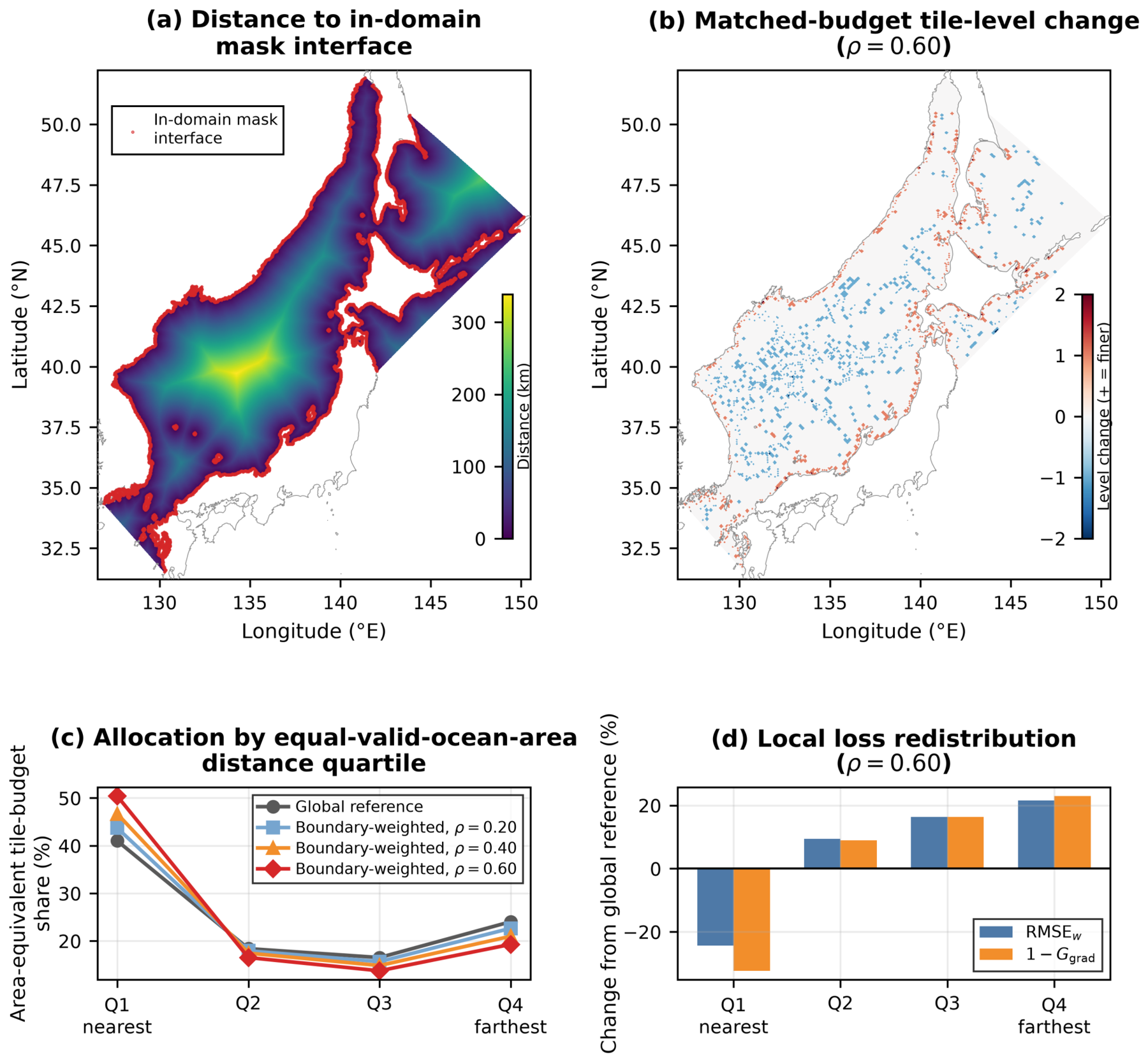
Fixed-budget model-mask-boundary allocation on M01. (
a) AEQD distance from each valid cell to the nearest in-domain valid–invalid mask-interface cell; Natural Earth linework is visual context only. (
b) Change in tile level for the
matched-budget partition relative to the global reference, with positive values denoting finer allocation. (
c) Area-equivalent share of the fixed tile budget assigned to four equal-valid-ocean-area distance quartiles for
, 0.20, 0.40, and 0.60. (
d) Percentage changes in quartile-local area-weighted RMSE and physical-gradient magnitude loss at
relative to the global reference. Negative values indicate lower local loss. All matched-budget cases use
; the same-base-tolerance (
) cost diagnostic is reported separately in
Supplementary Table S7.
Figure 10.
Fixed-budget model-mask-boundary allocation on M01. (
a) AEQD distance from each valid cell to the nearest in-domain valid–invalid mask-interface cell; Natural Earth linework is visual context only. (
b) Change in tile level for the
matched-budget partition relative to the global reference, with positive values denoting finer allocation. (
c) Area-equivalent share of the fixed tile budget assigned to four equal-valid-ocean-area distance quartiles for
, 0.20, 0.40, and 0.60. (
d) Percentage changes in quartile-local area-weighted RMSE and physical-gradient magnitude loss at
relative to the global reference. Negative values indicate lower local loss. All matched-budget cases use
; the same-base-tolerance (
) cost diagnostic is reported separately in
Supplementary Table S7.
Figure 11.
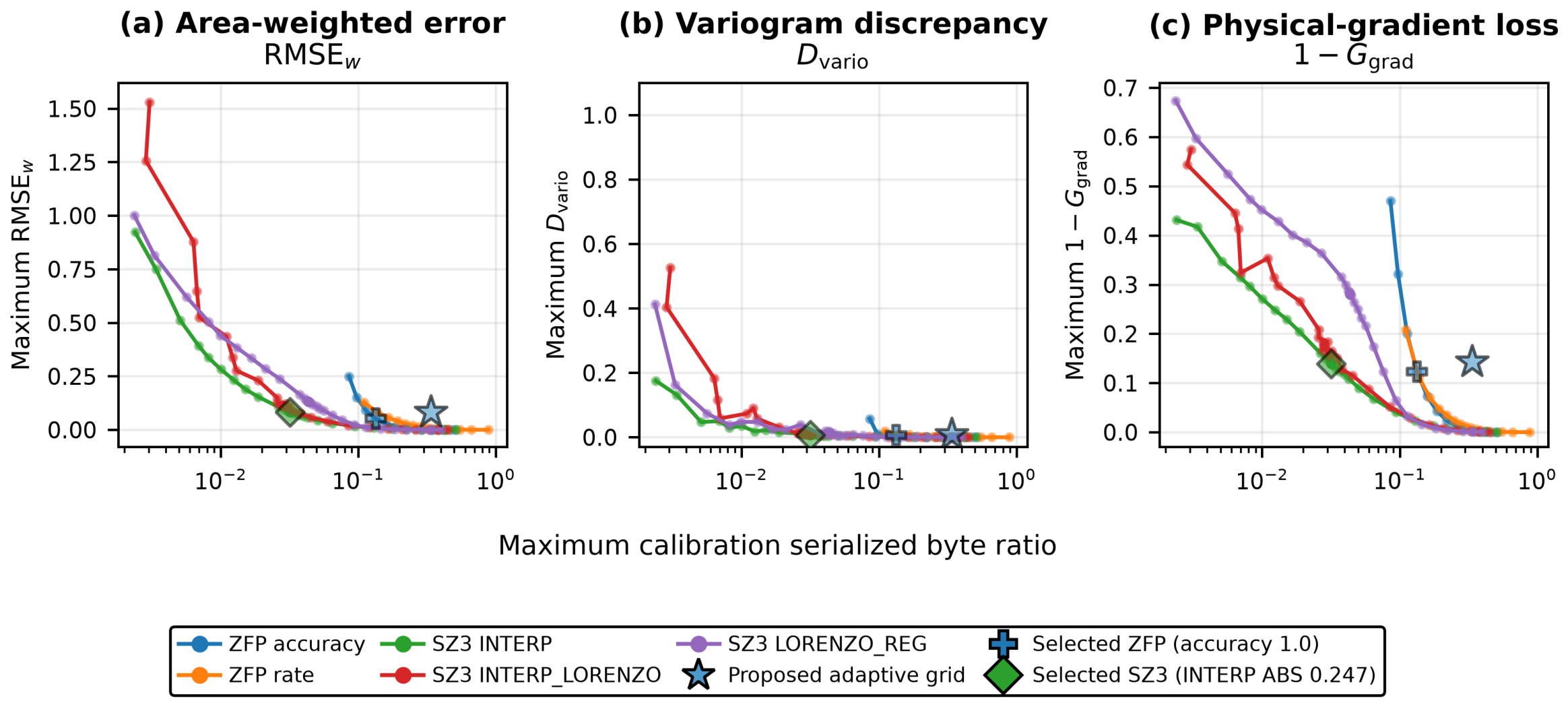
Calibration byte–fidelity operating regions for direct scientific codecs. Each panel plots maximum calibration serialized byte ratio against maximum (a) , (b) , or (c) . Curves show tested direct ZFP and SZ3 candidates. The star is the selected adaptive-grid reference and is not a member of either codec curve; the black-edged filled-plus and diamond markers identify the selected fidelity-constrained ZFP and SZ3 operating points, respectively. All operating-point selections use calibration fields only. ABS denotes the absolute-error bound; INTERP, INTERP_LORENZO, and LORENZO_REG identify the SZ3 interpolation, interpolation/Lorenzo, and Lorenzo/regression configurations, respectively.
Figure 11.
Calibration byte–fidelity operating regions for direct scientific codecs. Each panel plots maximum calibration serialized byte ratio against maximum (a) , (b) , or (c) . Curves show tested direct ZFP and SZ3 candidates. The star is the selected adaptive-grid reference and is not a member of either codec curve; the black-edged filled-plus and diamond markers identify the selected fidelity-constrained ZFP and SZ3 operating points, respectively. All operating-point selections use calibration fields only. ABS denotes the absolute-error bound; INTERP, INTERP_LORENZO, and LORENZO_REG identify the SZ3 interpolation, interpolation/Lorenzo, and Lorenzo/regression configurations, respectively.
Figure 12.
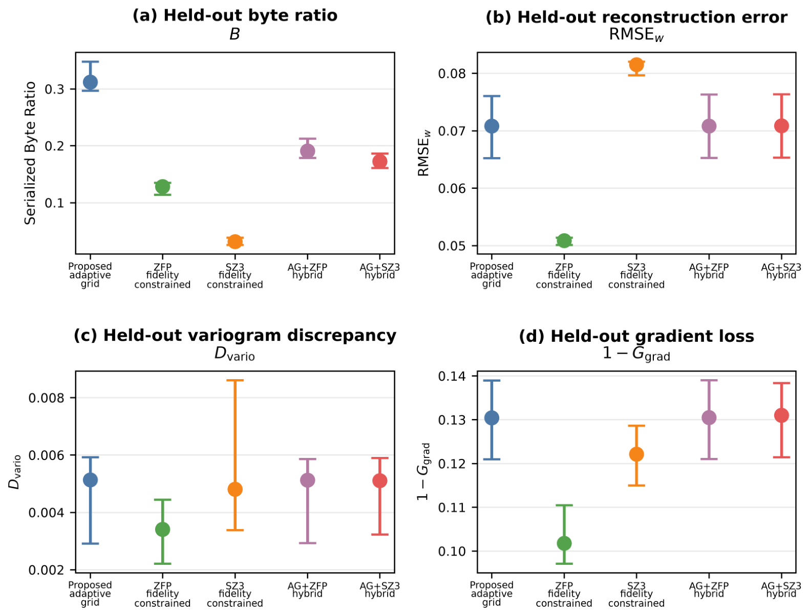
Primary held-out comparison of the proposed representation, direct codecs, and near-fidelity hybrids. Points are eight-field medians and bars are 95% field-bootstrap intervals for (a) serialized byte ratio, (b) area-weighted RMSE, (c) normalized semivariogram discrepancy, and (d) physical-gradient magnitude loss. AG+ZFP and AG+SZ3 retain the adaptive partition and compress only representative tile values.
Figure 12.
Primary held-out comparison of the proposed representation, direct codecs, and near-fidelity hybrids. Points are eight-field medians and bars are 95% field-bootstrap intervals for (a) serialized byte ratio, (b) area-weighted RMSE, (c) normalized semivariogram discrepancy, and (d) physical-gradient magnitude loss. AG+ZFP and AG+SZ3 retain the adaptive partition and compress only representative tile values.
Table 1.
Datasets, sampling design, and validation roles. The East Sea sequence contains twelve nominal monthly first-day fields; the VIIRS fields are dated monthly composites.
Table 1.
Datasets, sampling design, and validation roles. The East Sea sequence contains twelve nominal monthly first-day fields; the VIIRS fields are dated monthly composites.
| Dataset/Source | Variable and Transform | Grid/Support | Calibration–Held-Out Split | Role and Scope |
|---|
| KHOA ROMS, East Sea | Near-surface (1 m) potential temperature; Celsius; no transform | curvilinear grid; 130,131 common valid model-ocean cells; –E, –N | M01/M04/M07/M10 calibration; remaining eight nominal monthly first-day fields held out | Primary within-sequence evaluation and codec study |
| KHOA ROMS, East Sea | Near-surface salt; no transform | Same grid and model mask as temperature | Same four-to-eight split | Direct temperature-profile transfer and salinity- specific calibration |
| NOAA S-NPP VIIRS, California Current, 2024 | Monthly chlorophyll-a; primary | regular grid; calibration- valid intersection followed by field- valid intersection | Jan/Apr/Jul/Oct calibration; remaining eight monthly composites held out | Cross-region, cross-grid, satellite-source case study; raw-field and common-mask sensitivities |
| Proposed adaptive-grid profile-transfer analyses | , , , and for cross-variable comparisons | Complete nonoverlap, finite representatives, exact membership, and scale admissibility | Profiles fixed within each transfer test; partitions regenerated field by field | Held-out summaries describe the sampled sequences rather than an independent population |
Table 2.
Spatial comparators and matching rules.
Table 2.
Spatial comparators and matching rules.
| Method | Construction | Parameter Timing | Question Answered |
|---|
| Nearest tile-count uniform baseline | Fully valid blocks at one dyadic size plus singleton residual cells; nearest available tile count | Per field from discrete sizes | What trade-off does this strict-mask nearest-count rule produce? |
| Field-retuned local-RMSE quadtree | Area-weighted local-RMSE split tolerance binary-searched to the proposed tile count | Retuned on every field | At nearly equal tile count, what fidelity does an RMSE-oriented quadtree achieve? |
| Calibration-fixed local-RMSE quadtree | Local-RMSE splitting; one normalized tolerance selected by calibration Pareto–minimax | Fixed on held-out fields | How does a profile using local-RMSE splitting transfer? |
| -matched local-RMSE quadtree | Local-RMSE splitting with the selected proposed and per-field tile matching | fixed; tolerance per field | How much difference remains after sharing the maximum dyadic level? |
| Unconstrained-range quadtree | Same local block-range rule with an unconstrained structural maximum level and one calibration-selected threshold | Distinct maximum level and threshold fixed before evaluation; no realized-diameter filter | What behavior is obtained from a separately calibrated range-rule quadtree without the physical safeguard? |
| Proposed adaptive grid | Range-based dyadic partition, exact realized-diameter safeguard, and four-objective calibration minimax | Parameter profile fixed before held-out evaluation; partition regenerated per field | Can an explicit balanced operating profile transfer across the tested fields? |
Table 3.
Held-out medians with 95% field-bootstrap intervals for spatial methods. Lower is better for all four columns. Intervals summarize eight held-out fields and do not imply independent population sampling.
Table 3.
Held-out medians with 95% field-bootstrap intervals for spatial methods. Lower is better for all four columns. Intervals summarize eight held-out fields and do not imply independent population sampling.
| Method | | | | |
|---|
| Proposed adaptive grid | 0.2049 [0.1977, 0.2289] | 0.0708 [0.0653, 0.0760] | 0.0051 [0.0029, 0.0059] | 0.1304 [0.1210, 0.1389] |
| Nearest tile-count uniform baseline | 0.2038 [0.1504, 0.2573] | 0.3948 [0.3363, 0.4954] | 0.0373 [0.0205, 0.0745] | 0.4543 [0.4252, 0.4819] |
| Field-retuned local-RMSE quadtree | 0.2049 [0.1977, 0.2290] | 0.0808 [0.0763, 0.0880] | 0.0068 [0.0046, 0.0084] | 0.1484 [0.1397, 0.1603] |
| Calibration-fixed local-RMSE quadtree | 0.2208 [0.2104, 0.2600] | 0.0747 [0.0677, 0.0803] | 0.0058 [0.0051, 0.0088] | 0.1370 [0.1260, 0.1503] |
| -matched local-RMSE quadtree | 0.2049 [0.1977, 0.2289] | 0.0735 [0.0674, 0.0791] | 0.0057 [0.0040, 0.0082] | 0.1407 [0.1304, 0.1493] |
| Unconstrained-range quadtree | 0.2104 [0.1966, 0.2383] | 0.0702 [0.0651, 0.0761] | 0.0049 [0.0033, 0.0063] | 0.1291 [0.1203, 0.1380] |
Table 4.
Cross-variable and external-observation held-out medians. is dimensionless and supports within-table comparison more appropriately than raw variable-specific RMSE. Each row summarizes eight noncalibration fields. A profile is reported as ; target-specific profiles use only their four calibration fields.
Table 4.
Cross-variable and external-observation held-out medians. is dimensionless and supports within-table comparison more appropriately than raw variable-specific RMSE. Each row summarizes eight noncalibration fields. A profile is reported as ; target-specific profiles use only their four calibration fields.
| Dataset | Profile Definition | | | | |
|---|
| East Sea salinity | Direct temperature-profile transfer without recalibration: | 0.2298 | 0.0045 | 0.0021 | 0.1095 |
| East Sea salinity | Salinity-specific proposed profile: | 0.2651 | 0.0093 | 0.0063 | 0.0926 |
| California Current VIIRS transformed chlorophyll-a | Direct temperature-profile transfer without recalibration: | 0.7422 | 0.0040 | 0.0017 | 0.0380 |
| California Current VIIRS transformed chlorophyll-a | Chlorophyll-specific proposed profile: | 0.4055 | 0.0148 | 0.0068 | 0.1744 |
Table 5.
Primary held-out codec and hybrid comparison. Values are medians with 95% field-bootstrap intervals. Percentage changes are medians of field-paired changes relative to the proposed adaptive grid; negative values denote reductions.
Table 5.
Primary held-out codec and hybrid comparison. Values are medians with 95% field-bootstrap intervals. Percentage changes are medians of field-paired changes relative to the proposed adaptive grid; negative values denote reductions.
| Method (Selected Calibration Parameter) | B | | | | (%) |
|---|
| Proposed adaptive grid (, ) | 0.3121 [0.2968, 0.3481] | 0.0708 [0.0653, 0.0760] | 0.0051 [0.0029, 0.0059] | 0.1304 [0.1210, 0.1389] | 0 |
| ZFP fidelity-constrained (fixed accuracy 1.0) | 0.1284 [0.1139, 0.1347] | 0.0508 [0.0501, 0.0514] | 0.0034 [0.0022, 0.0044] | 0.1018 [0.0971, 0.1105] | −62.7 |
| SZ3 fidelity-constrained (INTERP ABS 0.247) | 0.0313 [0.0257, 0.0383] | 0.0815 [0.0797, 0.0820] | 0.0048 [0.0034, 0.0086] | 0.1221 [0.1150, 0.1286] | −89.8 |
| AG+ZFP, tile-mean tolerance 0.005 | 0.1907 [0.1788, 0.2126] | 0.0708 [0.0653, 0.0763] | 0.0051 [0.0029, 0.0059] | 0.1305 [0.1210, 0.1390] | −38.8 |
| AG+SZ3, LORENZO_REG ABS 0.005 | 0.1725 [0.1609, 0.1862] | 0.0709 [0.0653, 0.0764] | 0.0051 [0.0032, 0.0059] | 0.1310 [0.1214, 0.1384] | −46.0 |