Article

GPU-Based Solar Irradiance Estimation over Digital Surface Models Using Structurally Lossless Viewshed Compression

Faculty of Electrical Engineering and Computer Science, University of Maribor, 2000 Maribor, Slovenia
*
Author to whom correspondence should be addressed.
Remote Sens. 2026, 18(17), 3044; https://doi.org/10.3390/rs18173044
Submission received: 18 July 2026 / Revised: 1 September 2026 / Accepted: 3 September 2026 / Published: 6 September 2026

Abstract

High-resolution solar irradiance modelling over large 3D geospatial data is computationally demanding, and accounting for surface inter-reflection makes it even so. For computational efficiency it requires storing for every part of the surface, explicit knowledge of the other surfaces visible from it (its viewshed). The storage of each surface’s viewshed grows with both the dataset size and the angular resolution, and quickly becomes the dominant memory bottleneck. This paper presents a novel Graphics Processing Unit (GPU)-accelerated method for estimating solar potential over Digital Surface Models (DSMs) that model direct, diffuse and reflective irradiances. It keeps the viewshed information compact through a novel structurally lossless compression, i.e., a domain-specific encoding of remote sensing-derived visibility data that preserves exactly the visibility structure consumed by the radiative model, rather than a general-purpose integer coder. An ablation analysis over eight synthetic DSMs showed that the best compression scheme reached a compression ratio (CR) of up to ≈3.3, exceeding the general-purpose GPU baselines Binary Packing 32 and Elias-Fano on every dataset. On the largest DSM, whose 29.6 GB uncompressed viewshed exceeds the 24 GB device memory, compression kept the data resident and reduced the runtime from 6.7 h to 0.5 h. Finally, the proposed method was applied to LiDAR (Light Detection and Ranging)-derived DSMs for four distinct locations, with the results demonstrating its high applicability.

1. Introduction

In recent years, the volume of 3D geospatial data has grown rapidly, driven in large part by the widespread adoption of LiDAR (Light Detection and Ranging). Its high-resolution 3D scanning of the built and natural environment produces massive point-cloud datasets [1]. These datasets are transformed routinely into Digital Surface Models (DSMs) [2], triangle-based meshes [3], or voxelised volumetric representations [4], which serve as the geometric basis for a wide range of physically based simulations. The energy sector has particularly benefited from applications such as solar potential estimation [5,6], thermal-performance modelling of buildings [7], and urban-heat-island analysis [8]. These have all seen marked gains in accuracy and scalability from detailed 3D data, especially in morphologically complex urban environments [9]. As the spatial resolution and extent of these datasets keep increasing, however, the computational and memory demands of the underlying simulations grow significantly, so that efficiency and scalability become central concerns.
Solar-irradiance modelling over 3D geospatial data is a prime example of a simulation that is simultaneously high-resolution and large-scale, and many works have therefore turned to General-Purpose computing on Graphics Processing Units (GPGPU) to parallelise and accelerate it [2,10,11]. To contain the cost of visibility and shadow queries over large geospatial datasets, the Sparse Voxel Octree (SVO), a data structure used widely in computer graphics [12], has proven especially effective. Liang et al. [13] applied it to solar potential estimation with accurate shadowing over large 3D remote sensing datasets. Most of such approaches, however, model only direct and diffuse irradiance, together with shadowing. Reflective irradiance is more computationally intensive and additionally requires, for every surface unit (e.g., voxel), the explicit set of surrounding surfaces visible from it, i.e., its viewshed. While octree-based and similar methods [14] accelerate the search for this visibility information, they do not address the cost of retaining it. The viewshed is inherently memory-intensive, since its size scales with both the data resolution and the angular resolution of the visibility sampling. This information should not be discarded, because reflective irradiance has to be evaluated multiple times (e.g., every hour in a year). Storing it once and reusing it across all hours is therefore the only practical option. It should be noted that only the time-invariant viewshed data (i.e., the per-voxel visible surface indices) is stored and reused, while other data inputs required for irradiance estimation can change at every time step.
Reducing this memory demand is fundamentally a data-compression problem. Compression has been studied since the foundational works of Shannon [15], Fano [16], and Huffman [17], and is generally divided into lossless, near-lossless, and lossy classes [18]. Lossless techniques rely on the statistical properties of the data (e.g., Huffman [17], arithmetic [19] or asymmetric-numeral-system coding [20]), dictionary methods descending from LZ77 [21], and dedicated integer coders such as Golomb [22] and Golomb-Rice [23] coding. The former was originally devised for encoding runs in Run-Length Encoding (RLE) [18]. The choice of coding strategy, however, is only a part of the problem when compression is to be performed on a GPU. As GPU arithmetic throughput has continued to outpace the growth of on-device memory capacity and bandwidth, a broad range of GPU-accelerated workloads have become memory-bound rather than compute-bound [24]. Moreover, this has given rise to a substantial body of related work on GPU-oriented compression across several domains. Lightweight integer encoding [25,26] and lossless compression of integer data [27,28] have been developed. Mallia et al. [27] tested several approaches for integer data compression on a GPU, such as Binary Packing of 32 delta coded integers (BP32), and Gera and Kim [28] introduced a GPU-based implementation for Elias-Fano (EF) coding of integer values. Moreover, compression of floating-point data on GPU [29,30], and high-throughput GPU lossy compressors have been introduced, that trade controlled accuracy for higher compression [31,32]. Finally, a complementary axis separates the general-purpose from the domain-specific methods, the latter exploiting prior knowledge of the data to compress it more effectively. Such knowledge can permit a transformation that is not reversible with respect to the original representation, yet preserves all the information relevant to the target application, a property we refer to as structurally lossless compression. In the remote sensing context, this yields a domain-specific compression strategy for geospatial visibility data derived from LiDAR-based DSMs, which preserves exactly the visibility structure consumed by the physically based radiative model, in contrast to general-purpose integer coders.
In this paper we propose a novel GPU-accelerated method for estimating solar irradiance over DSMs, which, unlike prior work, incorporates first- and second-order reflective irradiance while keeping the per-voxel viewshed information in a compressed storage on a GPU. The main novel contributions are as follows:
  • A GPU pipeline is presented for solar irradiance over DSMs that augments direct and diffuse irradiance and shadowing with first- and second-order surface inter-reflection, evaluated per voxel for each hour over a full year.
  • A structurally lossless set-based compression scheme is proposed for per-voxel viewshed data compression with a bit-aware RLE (ba_RLE).
  • GPU-oriented binarisation of the ba_RLE tokens is proposed, by using a deterministic memory layout and an end-of-voxel guard.
  • A compact sun-band visibility bitmask is introduced that exploits the fact that, over a full year, the sun occupies only a narrow subset of the hemispherical viewshed represented by angular patches. Thus, the direct beam shadow test is reduced to a constant-time per-voxel bit lookup.
  • A comprehensive ablation analysis over eight synthetic DSMs is presented, where the compression ratio (CR), GPU memory footprint, runtime, and combined efficiency/throughput are considered across all bit-width-group RLE-based configurations.
The paper is organised as follows: Section 2 presents the methodology, comprising the theoretical background of the irradiance and reflection model, the proposed structurally lossless viewshed compression, and its GPU implementation for on-the-fly decompression. Section 3 reports an ablation analysis on synthetic DSMs and explores the compression, memory, and runtime behaviour of the proposed method, as well as the method’s applicability on LiDAR-derived DSMs. Section 4 concludes the paper and outlines directions for future work.

2. Methodology

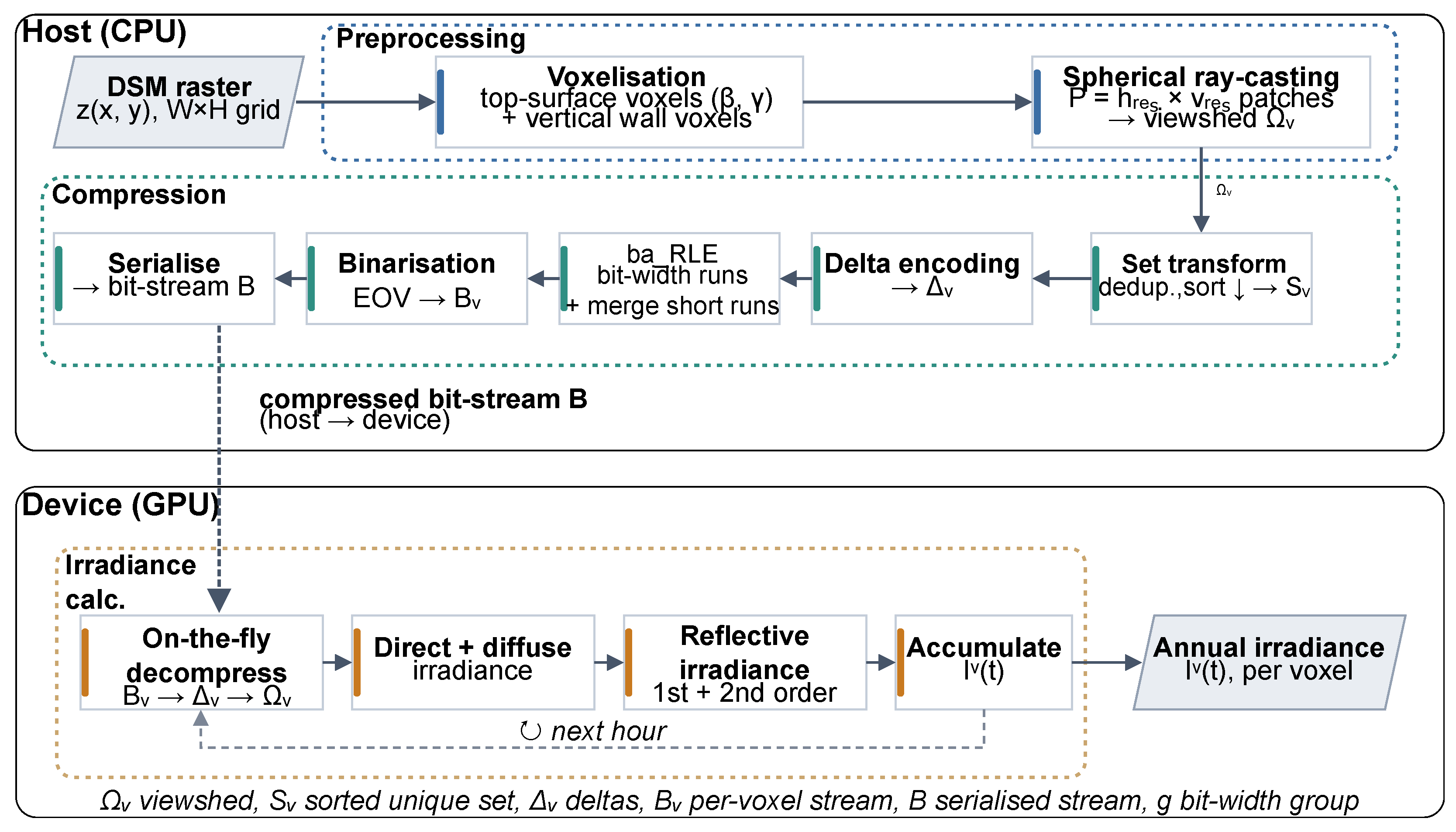
The proposed method’s overall workflow is summarised in Figure 1. DSM data preprocessing and the proposed viewshed compression are performed once on the host (CPU). Here, the DSM is voxelised, the viewshed of every voxel is obtained by spherical ray-casting, and the resulting visibility indices are compressed with the bit-aware RLE (ba_RLE), which is binarised into a compact binary stream. The stream is then transferred to the GPU, where it is decompressed on-the-fly inside the algorithm that evaluates the solar irradiance for every hour of the year. It should be emphasised that no new irradiance formulation is introduced, since the direct, the anisotropic Perez diffuse, and the area-based reflective components follow established formulations, unchanged with respect to our previously validated implementations [14,33]. The novelty of this work lies in how the visibility information these models consume is stored and retrieved.
Following this workflow, the section is organised into three parts. First, the Theoretical background formalises the DSM voxelisation, the viewshed computation, and the solar irradiance model. Second, Structurally lossless viewshed information compression introduces the proposed transformation of each voxel’s viewshed into a compact compressed stream. Third, the GPU implementation details how the compressed viewsheds are decompressed on-the-fly on the GPU.

2.1. Theoretical Background

The input DSM is a georeferenced raster of elevations z ( x , y ) sampled on a regular grid of size W × H with spatial per-pixel resolution V r e s in both horizontal directions. The maximum vertical height is denoted as Z. Each grid cell ( x , y ) defines a top-surface voxel v with position ( x , y , z ( x , y ) ) . The surface orientation at each top voxel is estimated via central finite differences over the four-connected neighbourhood:
z x z ( x + 1 , y ) z ( x 1 , y ) 2 V r e s , z y z ( x , y + 1 ) z ( x , y 1 ) 2 V r e s ,
from which the slope β and the surface azimuth γ angles are obtained, respectively, as
β = arctan z x 2 + z y 2 , γ = arctan 2 z x , z y ,
where γ is measured clockwise from the north and mapped to [ 0 , 2 π ) . The raster column index x increases eastwards and the row index y increases southwards, following the georeferenced raster order. Therefore, both the surface azimuth γ and the solar azimuth are measured clockwise from north in [ 0 , 2 π ) , and the outward unit normal follows as n = ( sin β sin γ , sin β cos γ , cos β ) [34].
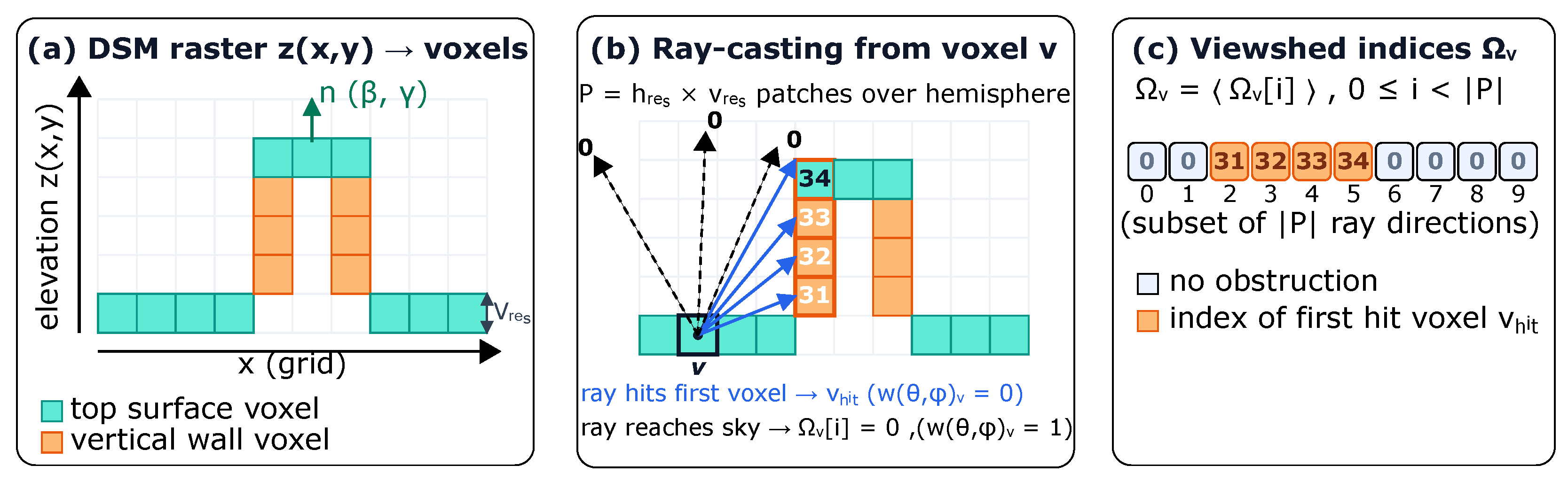
To capture vertical surfaces that are absent from the DSM representation, vertical voxels are generated wherever a significant height discontinuity exists between adjacent grid cells (see Figure 2a). For each surface voxel at position ( x , y ) with elevation z 0 = z ( x , y ) , the four cardinal neighbours are inspected. If a neighbour at ( x , y ) satisfies Δ z = z 0 z ( x , y ) > V r e s , then Δ z / V r e s vertical voxels are inserted along the vertical edge. The k-th vertical voxel is placed at elevation
z k w a l l = z ( x , y ) + k + 1 2 V r e s ,
with slope β w a l l = π / 2 and azimuth γ w a l l being equal to the surface voxel’s γ . The complete voxel set is then V = V t o p V w a l l , where | V | W × H × Z . | V t o p | = W × H represents top surface voxels and V w a l l the generated vertical voxels. In practice, | V w a l l | depends on the morphological complexity of the dataset, a flat terrain produces no vertical voxels, whereas dense urban areas with tall buildings yield | V w a l l | on the order of | V t o p | or larger.
For each voxel v V , a visibility preprocessing step is carried out by casting the rays into a full sphere discretised into | P | = p h r e s × p v r e s patches over 360 × 180 (Figure 2b). Each patch at azimuth–altitude coordinates { θ , ϕ } is assigned a binary visibility weight w ( θ , ϕ ) v { 0 , 1 } for the given voxel v. A ray in direction { θ , ϕ } v is tested against the voxel grid V. If an intersection is found, the patch is marked as obstructed, i.e., w ( θ , ϕ ) v = 0 , otherwise w ( θ , ϕ ) v = 1 . Given this visibility information, the direct solar irradiance received at v for a time instance τ is estimated as [34]:
I b v ( τ ) = J b ( τ ) cos θ i cos θ z w ( s θ , s ϕ ) [ Wm 2 ] ,
where J b [ Wm 2 ] is the direct horizontal irradiance, θ i is the angle of incidence, and θ z is the solar zenith angle, both computed from the tilt β and azimuth γ of v. The sun’s spherical coordinates { s θ , s ϕ } are obtained via the Position of the Sun Algorithm (PSA) [35].
Diffuse inter-reflections between the surfaces are approximated using area-based (form-factor) radiative exchange [34]. A first- and second-order reflected irradiance component is computed as [14]:
I r 1 v ( τ ) = v h i t S v α v h i t I b d v h i t ( τ ) π Γ ( v , v h i t ) A v h i t [ Wm 2 ] ,
I r 2 v ( τ ) = v h i t S v α v h i t I r 1 v h i t ( τ ) π Γ ( v , v h i t ) A v h i t [ Wm 2 ] ,
Γ ( v , v h i t ) = max ( 0 , n v · d ^ ) max ( 0 , n v h i t · ( d ^ ) ) | d | 2 ,
d = v h i t . x y z v . x y z , d ^ = d / | d | ,
where I b d v h i t ( τ ) = I b v h i t ( τ ) + I d v h i t ( τ ) is the combined direct and diffuse irradiance at the hit voxel. S v , the set of unique visibility indices obtained from Ω v through Equation (11), represents the voxel’s viewshed, i.e., the set of all surrounding voxels visible from v via ray-casting, where w ( θ , ϕ ) v = 0 because v h i t itself caused the obstruction. Building S v from Ω v is presented in Section 2.2. The projected surface area of a hit voxel is A v h i t = V r e s 2 , independently of the local slope, since every element of the voxelised viewshed is a cell-sized axis-aligned face. α v h i t is the surface diffuse albedo reflectance component. The geometric factor Γ accounts for the mutual orientation of the two surfaces through the dot products of the normals n v and n v h i t with the connecting unit vector d ^ , and for distance attenuation through the inverse-square term | d | 2 . No separate solid-angle weighting is required, since the product Γ ( v , v h i t ) A v h i t is the cosine-weighted solid angle subtended by the hit face at v, and the division by π completes the Lambertian form factor. The outward-pointing unit normal n v is derived directly from the given voxel’s β and γ . Higher-order reflections beyond the second bounce are neglected, as their energy contribution is typically negligible [34]. The total solar irradiance at voxel v for time instance τ is then:
I v ( τ ) = I b v ( τ ) + I d v ( τ ) + I r 1 v ( τ ) + I r 2 v ( τ ) [ Wm 2 ] .
The diffuse sky irradiance I d v ( τ ) is computed using the Perez anisotropic model, which additionally requires the horizontal diffuse irradiance J d [ Wm 2 ]  [36]. The solar potential of a voxel is defined as the corresponding irradiation accumulated over the year, i.e., the hourly discretised time integral of the modelled irradiance:
P v = h = 1 8760 I v ( τ h ) Δ τ [ Wh m 2 yr 1 ] , Δ τ = 1 h .
The solar potential P v is the standard decision variable in solar cadastre and photovoltaic planning applications, as it determines the expected annual yield of a candidate surface.
Since these calculations have to be done for each hour in a year, they are computationally expensive. It is therefore vital to store the viewshed in memory. However, as the number of voxels increases | V | , the size of v V | S v | becomes increasingly unsustainable. Hence, in this paper a novel compression method for voxels’ viewshed is proposed, as described, in more detail, in the next section.

2.2. Structurally Lossless Viewshed Information Compression

The viewshed associated with each voxel v V is denoted by Ω v and represented as a vector of non-negative integer values, Ω v = Ω v , i , where 0 i < | P | . Each value Ω v , i belongs to the domain R Ω , where R Ω = { 0 , 1 , 2 , , W · H · Z } . The value Ω v , i = 0 indicates that no voxel ν V obstructs the line of sight from voxel v along the considered ray, while a positive value encodes, offset by one, the linear three-dimensional grid index (Equation (13)) of the first occluding voxel along the ray. The upper bound is the size of the voxel space W · H · Z | V | , since the index addresses the regular grid rather than the compacted set V. Therefore the top-surface and vertical wall voxels alike are identified as visible elements, and the offset by one reserves the value 0 for unobstructed rays.
For compression purposes, a transformation T is defined that maps vector Ω v into a set of visibility indices, such that
S v = T ( Ω v ) = { Ω v , i 0 i < | P | , Ω v , i > 0 } ,
where T removes ordering and multiplicity information from Ω v as well as the zero entries corresponding to unobstructed rays. It retains only unique strictly positive visibility values, so that S v contains neither duplicates nor zeroes. Set S v is transformed further into a canonical representation by sorting its elements in descending order
S v = sort ( S v ) .
The information discarded by T is exactly the information the adopted radiative model does not consume. Equations (5)–(8) constitute an area-based summation over the set of visible surfaces, in which each visible element contributes once, weighted by its own area, its albedo, and the geometric factor Γ . The rays are merely the mechanism by which this set is discovered, as the number of rays striking the same voxel reflects the angular sampling density and the distance to that voxel, not the radiative exchange. Retaining the multiplicity and summing a surface once per intersecting ray would therefore count the same energy several times. Ordering may equally be discarded, since the summation is commutative. What must be preserved is the identity of the visible surfaces, and that is preserved exactly. This is what structurally lossless expresses in this paper.
Delta encoding Δ v = Delta ( S v ) defined as
Δ v , 0 = S v , 0 , Δ v , i = S v , i 1 S v , i , 1 i < | S v |
is applied after that. Since S v is strictly decreasing and contains unique integer values, all the elements of Δ v are positive integers. However, in general, the magnitude of Δ v , i Δ v may exceed the value 256, which can be represented within a single byte. This makes the application of conventional compression techniques challenging for the following reasons:
  • Statistical compression methods are not suitable, as maintaining per- Ω v statistical models would require excessive memory, while global statistics fail to capture the variability of individual visibility profiles.
  • Dictionary-based approaches would require maintaining separate dictionaries for each v V , which is inefficient in both memory usage and initialisation cost. Furthermore, a global dictionary does not reflect the local structure of individual visibility sets.
  • Golomb and Golomb–Rice coding provide efficient integer compression in sequential settings. However, their variable-length output is poorly suited for GPU implementations due to the lack of deterministic memory alignment.
This motivates the use of dedicated encoding schemes suitable for GPU memory layouts and parallel processing, as described in Algorithm 1. The input to the function is the array of visibility indices Ω v , whose length is | P | . The functions in lines 2 and 3 perform the transformation T , which discards the zero entries and the duplicates, and sort the resulting unique indices in decreasing order. Delta encoding is realised according to Equation (12). The encoding is performed in lines 5 and 6 as explained in the continuation.
Algorithm 1: Compression of visibility indices Ω v .
Remotesensing 18 03044 i001

2.2.1. Bit-Aware Run-Length Encoding

RLE is an intuitive data compression method, which performs well in specific situations, i.e., when identical values occur consecutively in the data stream. These sequences of repeated values are referred to as runs. RLE is used in various image formats [37] and elsewhere [38]. RLE compression represents the input data using tokens consisting of two elements: the run length and the repeated value. However, RLE performs poorly when repetitions are rare or absent. Runs can be increased by applying transformation techniques such as the Burrows-Wheeler transform [39]. This approach is effective when correlations exist in the data, or when the symbol alphabet of symbols is small [40]. However, efficient GPU implementation of the Burrows-Wheeler transform is non-trivial, due to its inherent suffix sorting requirements and irregular memory access patterns. In our case, the elements Δ v , i Δ v can take arbitrary numbers from the range R Ω , while runs of identical elements are typically short. However, runs of elements sharing the similar bit-width representation occur significantly more frequently. This property is exploited in the proposed bit-aware RLE (ba_RLE). Each element Δ v , i is assigned a group index g { 0 , , 4 } based on its bit-width requirement:
  • Group g = 0 : Δ v , i < 2 4 .
  • Group g = 1 : 2 4 Δ v , i < 2 8 .
  • Group g = 2 : 2 8 Δ v , i < 2 16 .
  • Group g = 3 : 2 16 Δ v , i < 2 24 .
  • Group g = 4 : 2 24 Δ v , i < 2 32 .
These groups define a logarithmic binning of integer magnitudes.
The ba_RLE method operates in the following passes:
1.
Determination of bit-aware runs of Δ v , i according to the introduced groups, with storage of this information in an intermediate array T v .
2.
Optimisation of T v by removing short runs, if adequate.
The number of bits b i required to represent each Δ v , i is given by b i = log 2 ( Δ v , i ) + 1 . Each b i determines the corresponding group g implicitly according to the defined binning. The runs l of identical group indices are then determined. The token ( g , l ) , consisting of the group index and the run length, is inserted into the token stream T v = ( g t , l t ) , 0 t < | T v | , where | T v | | Δ v | .
Finally, let us consider the short example in Figure 3.
As can be seen, some tokens represent only one element. Such tokens reduce the efficiency of encoding, which is why merging neighbouring tokens is attempted. Let us suppose that the considered token is ( g t , l t ) . Consequently, its neighbouring tokens are ( g n , l n ) , where n = t ± 1 . Token ( g t , l t ) can be merged with a neighbouring token when
1.
l t = 1 and g t + 1 = g n , or
2.
g t = g n .
  • If either condition is satisfied, token ( g t , l t ) is removed from T, while the neighbouring token ( g n , l n ) is updated to ( g n , l n + l t ) . When t = 0 or t = | T | 1 , only the next or previous token is considered, respectively. In our example,
    T = ( 3 , 1 ) ( 1 , 1 ) ( 2 , 1 ) ( 1 , 1 ) ( 2 , 1 ) ( 0 , 6 ) ( 1 , 1 ) ( 0 , 7 ) .
    The first token ( 3 , 1 ) cannot be merged with its neighbour ( 1 , 1 ) , since 3 + 1 1 . The second token ( 1 , 1 ) satisfies the first condition and is therefore merged with its right-hand neighbour, giving
    T = ( 3 , 1 ) ( 2 , 2 ) ( 1 , 1 ) ( 2 , 1 ) ( 0 , 6 ) ( 1 , 1 ) ( 0 , 7 ) .
    Similarly, the next token ( 1 , 1 ) is merged with its right-hand neighbour ( 2 , 1 ) to obtain
    T = ( 3 , 1 ) ( 2 , 2 ) ( 2 , 2 ) ( 0 , 6 ) ( 1 , 1 ) ( 0 , 7 ) .
    Checking token ( 2 , 2 ) is also successful, as the second condition is satisfied: the group indices match those of its left-hand neighbour. After merging
    T = ( 3 , 1 ) ( 2 , 4 ) ( 0 , 6 ) ( 1 , 1 ) ( 0 , 7 ) .
    The process terminates as no further merging of tokens is possible.

2.2.2. Binarisation

The sequence of ba_RLE tokens stored in T v , together with Δ v , is binarised in this step. Binarisation is performed with consideration of the GPU memory model, with an emphasis on efficient byte-aligned memory access. However, since byte-aligned bit-packing can also be realised on the GPU efficiently, it is applied as well. As the binarisation of the elements Δ v , i Δ v is straightforward, the binarisation of ba_RLE tokens ( g t , l t ) , where 0 t < | T v | , is explained in the following.
The first ba_RLE parameter takes five different values representing the defined groups. For this reason, three bits are required in a standard binary encoding. For example, g = 0 is encoded as 000, g = 1 as 001, g = 2 as 010, g = 3 as 011, and g = 4 as 100. Since three codewords remain unused, the code 110, referred to as End Of Voxel (EOV) data, is used to indicate the end of T v . Eight consecutive values of g t are then bit-packed into three bytes, followed by a sequence of eight bytes encoding the run lengths l t . As each l t is encoded with one byte, the maximum run length that can be encoded is 255. If a run is longer, it is split into multiple parts, taking care that none of the runs is zero. After that, the consecutive elements forming Δ v are encoded.
Let us consider the example in Figure 4 using the initial sequence of tokens T v from Figure 3.
The first three bytes are filled with the values of g t , in this case for 0 t < 8 , using a three-bit binary encoding. After that, eight bytes containing the run lengths l t , 0 t < 8 , follow. Finally, the eight elements Δ v , i , 0 i < 8 , are written using the appropriate number of bytes as specified by the corresponding values of g t . Note that two consecutive values are bit-packed into one byte when g t = 0 . In our example, there are seven such values represented by the token t 7 = ( 0 , 7 ) . As the run length is odd, only the four most significant bits of the last byte in the example shown in Figure 4 are used and the values of the four least significant bits are unimportant.
Finally, all the necessary data needed to restore the visibility indices are serialised into the binary stream B, as demonstrated in Algorithm 2.
The voxel space data are first stored in B using 32 bits per coordinate in line 3. All voxels v in the voxel space V are then visited. Those that contain visibility indices are processed further. The corresponding voxel index is then stored in B as a 32-bit integer, followed by the bitstream B v obtained from Algorithm 1, in lines 6 and 9, respectively.
Note that it is straightforward to determine voxel coordinates from a voxel index in the case of a defined raster scan of the voxels. If the index is determined according to Equation (13),
v = x + y · W + z · W · H
then the voxel coordinates are determined according to Equation (14).
x = v mod W y = v W mod H z = v W · H
Algorithm 2: Constructing final bitstream B.
Remotesensing 18 03044 i002

2.2.3. Decoding Compressed Visibility Indices

The decoder is asymmetric with respect to the encoder. The algorithm (see Algorithm 3) reads the binary stream B in Line 2 and then reconstructs the metadata in Line 3, including the size of the voxel space (W, H, Z) and the number of voxels | V | with visibility indices. The number of bytes needed by ba_RLE to store the actual values of the visibility indices is maintained in the array Lengths , and the length of Lengths is | V | . The main loop then assigns each binary stream B v independently from the serialised bitstream B in Line 5. ba_RLE encoded values are reconstructed in Line 6. They are used to calculate the actual values of the visibility indices S v by performing the inverse delta transform in Line 7.
Algorithm 3: Decoding.
Remotesensing 18 03044 i003
The decoding process is shown in Algorithm 4. The pointer BvIndex is used for controlling the movement through the bitstream B v . Three bytes are read from B v , which, as explained in Section 2.2.2, contain eight codes g t . In the case that there are fewer groups, this is indicated by the guard EOV. BvIndex is incremented by 3 after that in either case in Line 7. The function in Line 8 fills the array L, which contains the actual lengths of the runs. According to the explanation above, one byte is used for storing each length. Normally, eight consecutive bytes are read. However, if G contains the guard EOV, the array is shorter. According to this, BvIndex is also incremented within the function. With the information on the groups and the run-lengths, the actual values are reconstructed within the loop (Lines 10 to 13). The function in Line 12 performs this task by incrementing BvIndex according to the actual code g t . The reconstructed values are then appended to the array Δ v in Line 13. The reconstruction of Δ v values continues until EOV is detected in G.
Algorithm 4: Decoding ba_RLE encoded values of Δ v .
Remotesensing 18 03044 i004

2.3. GPU Implementation

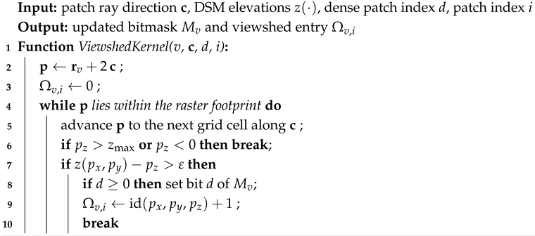
The pipeline is executed on the GPU with one thread assigned to each voxel v V , where the threads are grouped into blocks of 256, and the launch grid contains | V | / 256 blocks. The annual irradiance of every voxel, including inter-reflection, is obtained by launching three lightweight GPU-based algorithms (i.e., kernels) repeatedly, that share a small collection of device buffers. Two design choices make this tractable at scale and are detailed below: (i) the shadowing required by the direct component is reduced to a constant-time per-voxel bit test, and (ii) the per-voxel viewshed required by the reflective component is decompressed on the fly inside the reflection kernel, so that the uncompressed S v is never expanded in the device memory.
Data related scalars are placed in the GPU constant memory, namely: the DSM raster dimensions, the voxel count | V | , the angular resolution together with the number of hemispherical patches, and the maximum elevation. Quantities that depend on time but not on the voxel are precomputed once for all 8760 h of the year and uploaded as constant arrays, namely: the solar position { s θ , s ϕ } from the PSA, the horizontal direct and diffuse irradiances J b and J d . The remaining geometry resides in the global memory: the DSM elevations, the per-voxel slope β and azimuth γ , the elevations of the vertical voxels V w a l l , the visibility bitmask described below, and three per-voxel floating-point accumulators holding, respectively, the hourly direct-plus-diffuse irradiance, the hourly reflected irradiance, and the running annual total P v . The viewshed is uploaded only in compressed form, where the serialised stream B, i.e., the concatenation of the per-voxel streams B v , is stored as a byte array. The given stream is accompanied by an offset array of | V | + 1 entries that delimits the byte range of each B v . This offset array is the device-side counterpart of the AssignBitsToVoxels step of Algorithm 3, and the compressed stream is the only representation of the viewshed kept on the GPU.
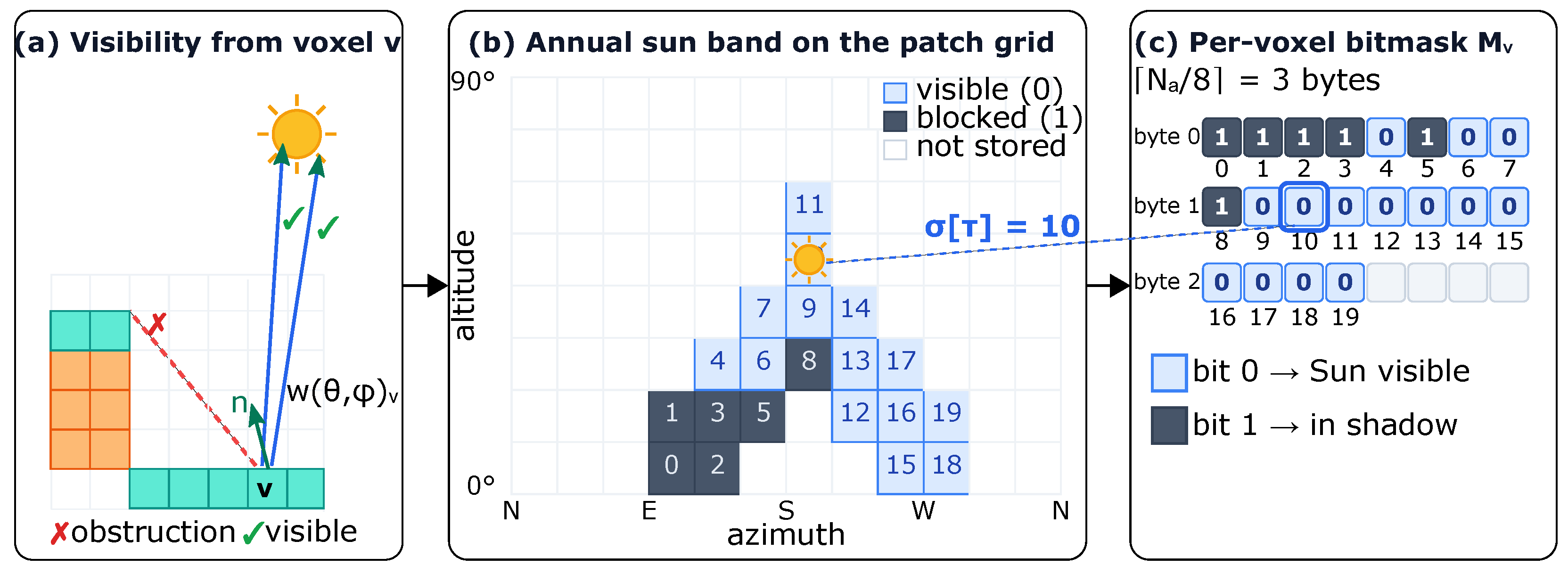
Because the reflection loop visits every voxel at every daylight hour, the shadow test of the direct beam should be inexpensive. The key observation is that, over a full year, the Sun sweeps only a narrow band of the upper hemisphere, where among the | P | patches, only a small subset A is ever occupied by the Sun. It is therefore sufficient to store, for each voxel, the visibility of these sun-reachable patches rather than the entire viewshed (Figure 5a,b). Every patch in A is assigned a dense, consecutive index, and for each voxel v a bitmask M v of N a = | A | bits is kept, packed into N a / 8 bytes (Figure 5c). A set bit marks a sun direction that is obstructed for v (i.e., w ( θ , ϕ ) v = 0 ), while a cleared bit marks a visible one ( w ( θ , ϕ ) v = 1 ). The bitmask is populated during the hemispherical ray-casting visibility step, which is launched once per patch direction over all the voxels. At the first occluder along the ray, the kernel sets the corresponding bit whenever the patch is sun-reachable. This GPU kernel is summarised in Algorithm 5. The kernel therefore fills Ω v as a | P | -length vector, one entry per patch, with Ω v , i = 0 where the ray escapes to the sky. Duplicates and zeros are removed only later, by the transformation T (Equation (11)).
Algorithm 5: Hemispherical ray-cast with sun-band bitmask.
Remotesensing 18 03044 i005
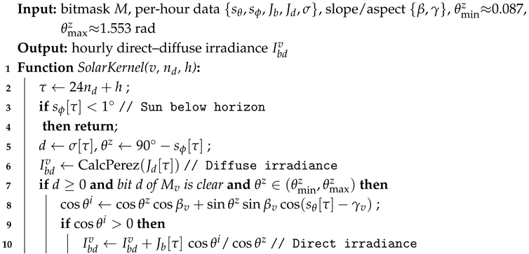
Since this step requires up to | P | potential candidate indices per voxel before compression, it is executed out-of-core over multiple voxel chunks. Hence, only one chunk’s uncompressed viewshed is ever within GPU memory while its indices are encoded into B on the host. A per-hour table σ maps each hour to the dense index of the patch the Sun then occupies, or to a sentinel when the Sun is below the horizon. Shadow determination is thus reduced to O ( 1 ) : for the current hour the solar kernel reads this index and tests the single corresponding bit of M v . Beforehand, the diffuse irradiance I d v is estimated using the anisotropic Perez model [36], which is evaluated regardless of whether the corresponding bit of M v is set, so that a surface shadowed from the direct beam still receives sky diffuse irradiance. If the bit is cleared, the direct irradiance I b v is estimated as well. The full kernel for estimating both irradiances is given in Algorithm 6. The zenith bounds in Algorithm 6 are numerical guards rather than physical limits. The upper bound ( θ max z 89 ) keeps the beam ratio cos θ i / cos θ z well conditioned. Consequently, the time steps at which the solar zenith angle exceeds θ max z 89 are excluded from the direct beam calculation. Their contribution to the annual solar irradiation is assumed to be negligible, since at such low solar elevations the beam is strongly attenuated by the long atmospheric path length and is, in practice, also obstructed by the surrounding terrain and buildings. Additionally, the lower bound ( θ min z 5 ) excludes the immediate neighbourhood of the zenith, where the azimuthal extent of a hemispherical patch degenerates and the bitmask index would be ill-defined.
Algorithm 6: Direct and diffuse irradiance with shadowing.
Remotesensing 18 03044 i006
The reflective component, by contrast, requires the explicit set of visible voxels S v . The reflection kernel, given in Algorithm 7, assigns one thread to each voxel v, locates the byte range of B v within B from the offset array, and decodes it inline following the same ba_RLE reconstruction as Algorithm 4. For each block, three bytes are unpacked into up to eight three-bit width-group codes terminated by the EOV guard, and one length byte is read per run. The delta payload of every run is decoded according to its group, as nibble-packed pairs for the smallest group and as big-endian byte tuples otherwise. The inverse delta Ω Ω prev δ reconstructs each visibility index in turn, the first decoded value being the largest index of the descending set. Each reconstructed index identifies one visible voxel v h i t , where the kernel forms the connecting vector d , evaluates the geometric factor Γ ( v , v h i t ) from the two surface normals and the inverse-square distance. The contribution α v h i t I b d v h i t Γ ( v , v h i t ) A v h i t / π is then added to a GPU memory register, where I b d v h i t is read from the hourly direct-plus-diffuse buffer produced by the solar kernel. Because decoding and accumulation are fused, every visibility index lives only briefly in a register and is discarded after use.
Algorithm 7: On-the-fly viewshed decompression fused with reflective-irradiance accumulation.
Remotesensing 18 03044 i007
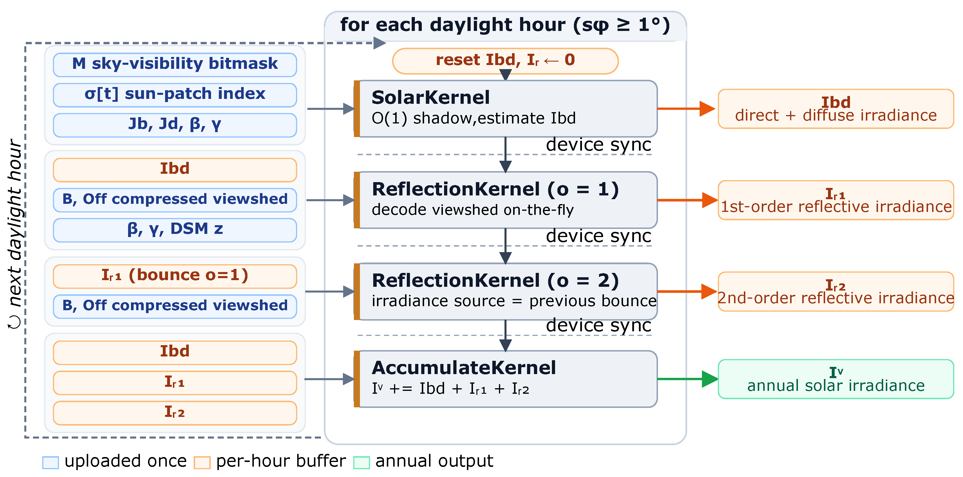
For each hour at which the Sun is above the horizon, the hourly accumulators are cleared and the kernels are launched in sequence, as illustrated in Figure 6. The solar kernel (Algorithm 6) writes the hourly irradiance I b d v = I b v + I d v using the constant-time shadow test. The reflection kernel (Algorithm 7) is then applied to obtain the first-order reflected irradiance I r 1 v from I b d , and is re-applied with I r 1 as its source to obtain the second-order I r 2 v . A device synchronisation separates dependent kernels. Finally, the accumulation adds the hourly irradiance contributions into the annual total P v of Equation (10), i.e., the voxel’s solar potential.

3. Results and Discussion

To isolate the impact of the compression configuration from the geospatial surfaces’ morphology, the experiments were conducted as an ablation study over a controlled family of eight synthetic DSMs of progressively increasing complexity. The evaluation focused on the following:
(i)
Compression effectiveness, measured by the compression ratio CR = | S v no _ compr | / | S v compressed | , where S v no _ compr represents viewshed indices without duplicates or zeroes.
(ii)
GPU memory footprint of the on-device viewshed storage buffer.
(iii)
The total GPU runtime.
(iv)
Combined quality-speed metrics that quantify whether the storage savings translate into useful computational throughput.
Lastly, based on the best RLE compression configuration, experiments on real 3D LiDAR derived DSMs for various locations were done as will be shown in the continuation. All experiments were done on an NVIDIA RTX 4090 (24 GB GDDR6X with CUDA 12.6) and AMD Ryzen 9 7950X CPU. Each reported time is the mean of 10 runtimes, using only runtimes within the 95% confidence interval.

3.1. Ablation Analysis over Synthetic DSMs

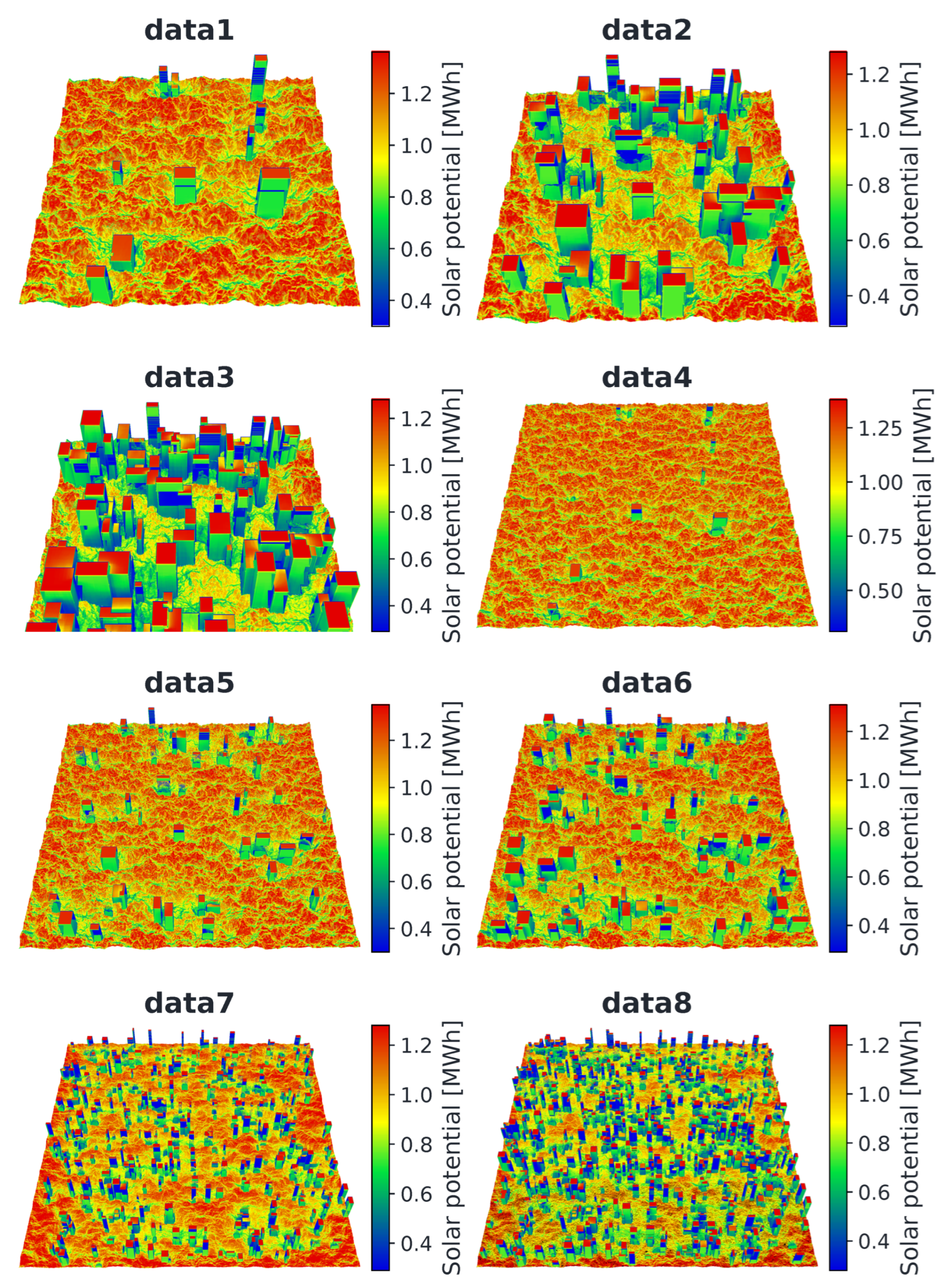
The eight synthetic DSMs, denoted data1 to data8, span an order of magnitude in voxel count and are summarised in Table 1. Their annual solar potential is visualised in Figure 7. Typical meteorological year (TMY) [41] of diffuse and direct hourly measurements from Maribor, Slovenia, were used as the irradiance input for all of them. They were generated by combining low-frequency Perlin-noise terrain with a controlled population of cuboidal buildings of increasing density and height variance. The resolution of the voxels was set at V r e s = 1 m3, the albedo was set as constant α = 0.2 , and viewshed discretisation was fixed at p h r e s = p v r e s = 64 patches across all the experiments.
For the ablation analysis, eight configurations of the compression pipeline were compared with the baseline. The baseline no_compr stores S v uncompressed in 32-bit integer form. The RLE variants are denoted rle_〈bw〉, where the suffix bw lists the active bit-width groups. For example, rle_4_16_24_32 activates the 4-, 16-, 24-, and 32-bit RLE groups (i.e., groups g = 0 to g = 4 ). These variants thus span all the non-empty subsets of { 4 , 8 , 16 } combined with the { 24 , 32 } as fallback. This enables us to isolate the marginal contribution of each RLE variant both to compression effectiveness and to the runtime decompression cost. Furthermore, comparison to two general-purpose GPU based integer compression methods were performed, namely BP32 [27] and Elias-Fano (EF) method [28].
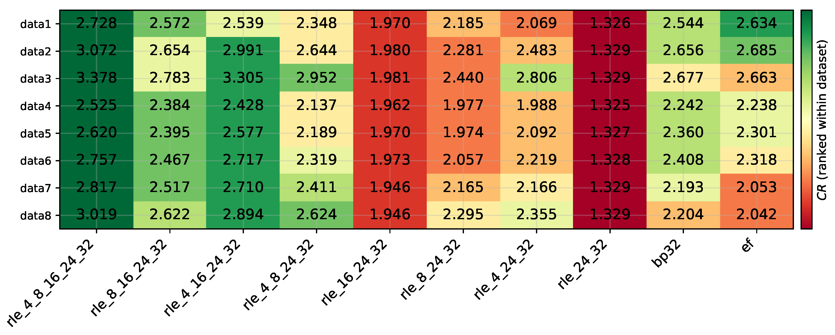
Figure 8 shows the CR across all dataset-variant combinations, where the horizontal stability of the colour bands evidences the near-invariance of CR with respect to dataset size. Three further trends stand out. The 4-bit group is the dominant compression lever: activating it raises rle_16_24_32 ( CR 1.97 ) to rle_4_16_24_32 ( CR 2.43 3.31 ), and rle_8_16_24_32 (≈2.38– 2.78 ) to the full rle_4_8_16_24_32 (≈2.53– 3.38 ). The complete rle_4_8_16_24_32 attained the highest ratio on every dataset, whereas as expected the rle_24_32 had the weakest ( CR 1.33 ), confirming that the lower bit-width groups, not the 24- or 32-bit fallback, drove the overall compression. Both general-purpose baselines were also surpassed on every dataset, with BP32 reaching CR 2.19 2.68 and EF ≈2.04– 2.69 .
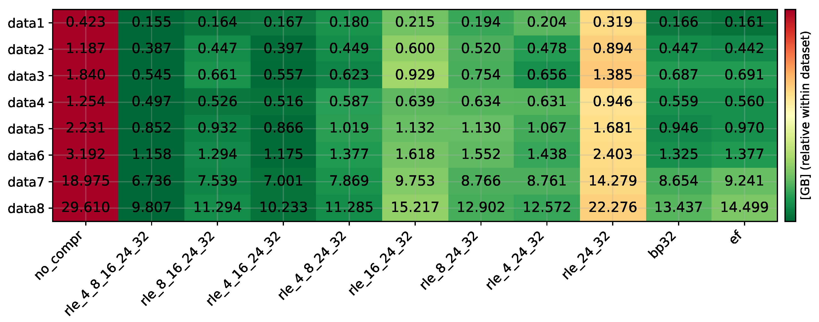
Figure 9 reports the GPU memory consumed by the neighbour-storage buffer. For the baseline no_compr, the footprint scales linearly with V, rising from 0.423 GB at data1 to 29.610 GB at data8. The full rle_4_8_16_24_32 scheme was the lightest configuration on all eight datasets, e.g., 0.155 GB vs. 0.423 GB on data1 and 9.807 GB vs. 29.610 GB on data8, a ≈63% on data1 and ≈66% on data8. In contrast, the rle_24_32 carried the largest residual footprint among the compressed variants. In practical terms, the achieved CR extends the reach of the method directly: at data8’s per-voxel viewshed footprint (≈2.5 KB uncompressed, ≈0.8 KB compressed), a 24 GB device can keep resident the viewshed of 9.7 million voxels uncompressed, but 29 million voxels compressed. This corresponds to roughly three times larger areas at the same spatial and angular resolution. data8 itself ( 11.9 million voxels) already exceeds the uncompressed budget, with the runtime consequences quantified below.
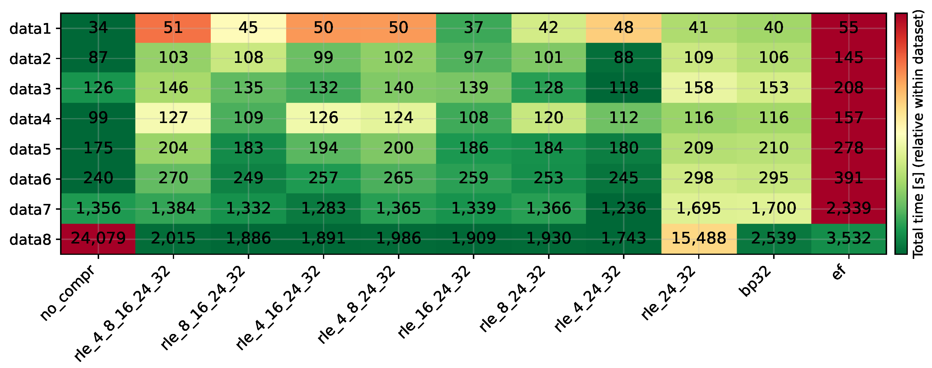
Figure 10 shows the total time T Tot breakdown for all the variants and baseline. This time includes all the steps from viewshed estimation, data compression and irradiance estimation with on-the-fly decompression, including all data transfers between the host and the device. During these tests, the GPU processor clock was fixed at 2235 Mhz, in order to mitigate possible fluctuations further. As expected, most RLE variants were slower than no_compr, but the relative gap narrowed with increasing | V | . The best configurations were rle_4_24_32 and rle_16_24_32, whose data6 runtimes ( 244.6  s and 259.1  s) lie within 2– 8 % of the baseline ( 240.4  s), while rle_24_32 and the full rle_4_8_16_24_32 were the most expensive, up to 1.5 times. BP32 remained competitive with the weakest RLE variants ( 1.17 1.25 times the baseline), whereas EF was the slowest method overall at 1.58 1.72 times, its costlier decoding outweighing a CR comparable to that of BP32. On data8 the trend reversed entirely: the uncompressed neighbour storage ( 29.6  GB) no longer fits into the device memory, so the GPU device driver spilled the excess into the shared system memory. Consequently, every compressed variant completes in 0.5 4.3  h against 6.7  h for no_compr.
To distill the storage-speed trade-off into a single comparable score, we evaluated the results further using two derived metrics adapted from the lossless-compression benchmarking literature [31]:
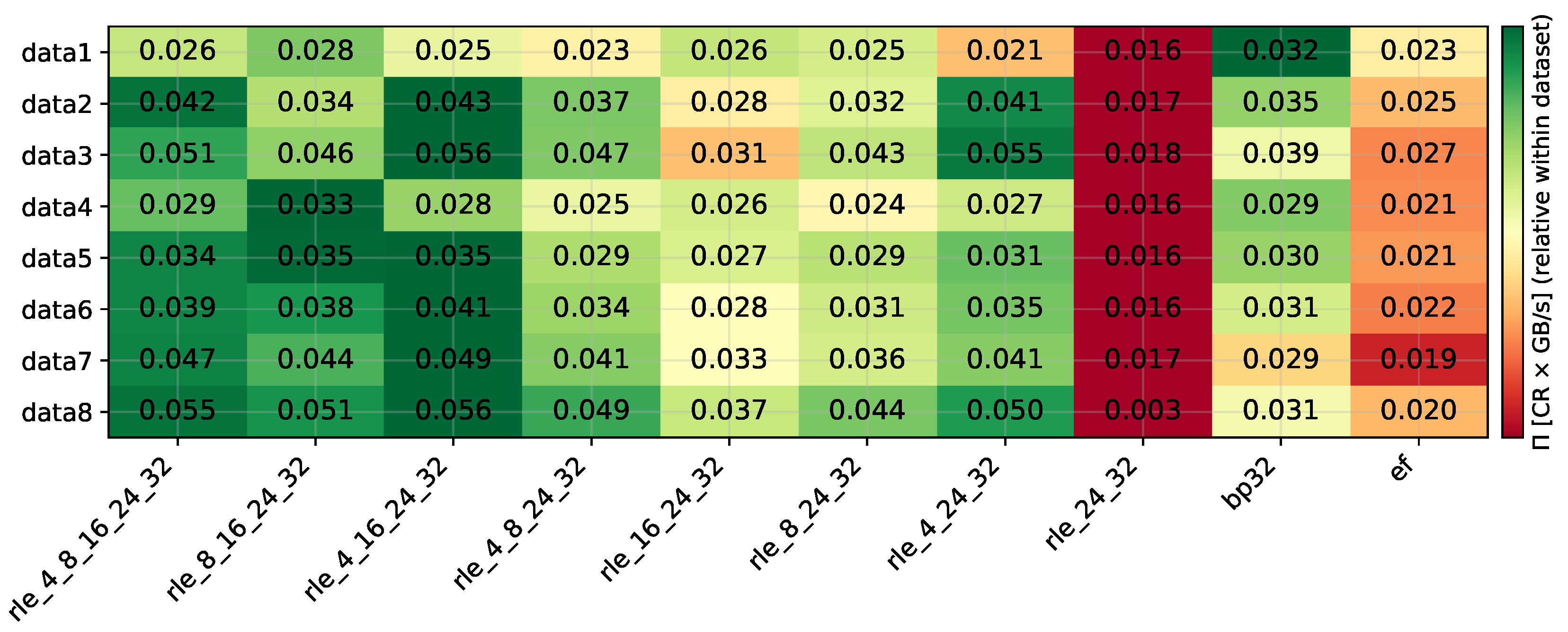
E = S d | S v compressed | , Π = CR · S d ,
where S d = | S v no _ compr | / T GPU [MB/s] is the decompression throughput, defined here as the volume of original viewshed data decompressed effectively by the GPU per unit time.
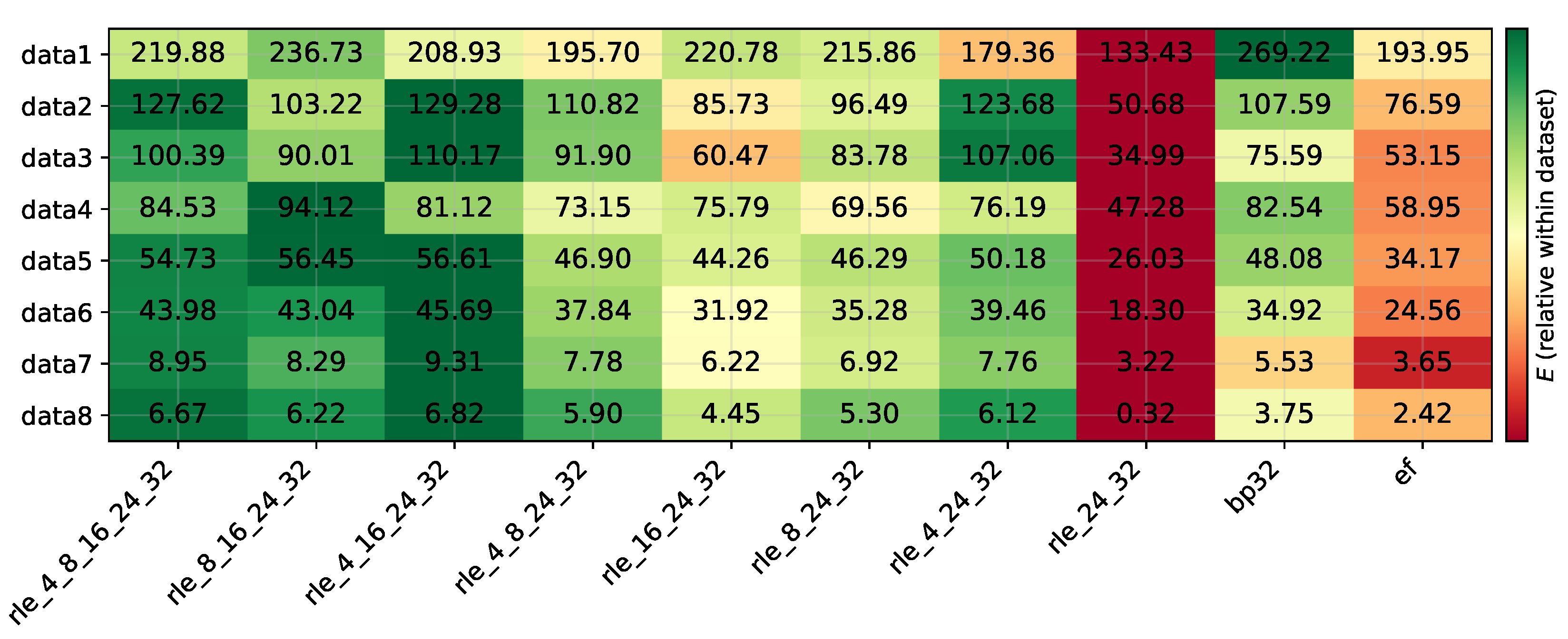
The metric E reflects how many original bytes per second are restored, normalised by the size of the compressed storage. The results are shown in Figure 11. The metric is most informative as a relative ranking, where it discriminates between variants on the basis of how much compression they extracted per second of effective work. In practice, RLE variants with lower groups enabled were the most efficient. The rle_24_32 was consistently the least efficient, ranking last on every dataset behind BP32 and EF as well.
On the other hand, the metric Π (with units of GB/s) represents the joint reward, since a configuration scores well only if it is simultaneously high-compression and high-throughput. As shown in Figure 12, Π increased broadly with dataset size for the RLE variants. Although not monotonically, e.g., rle_4_16_24_32 rises from 0.0245 to 0.0561  GB/s between data1 and data8, with the favourable data3 scene breaking the trend. This again reflects the amortisation effect, where as | V | grows, both the throughput term S d and the bandwidth-effective work per token rise, while CR remains stable. In contrast, BP32 stays nearly flat ( 0.029 0.039  GB/s) and EF even declines, so the gap in favour of the proposed scheme widens with scale. As expected from the previous results, by this combined measure variants with lower RLE groups enabled were the strongest, while rle_24_32 had the lowest throughout.
To verify that the compression did not affect the estimated irradiance, the pipeline was run twice on every dataset, once with the uncompressed viewshed storage (no_compr) and once with the rle_4_8_16_24_32 variant. The resulting solar potentials were then compared voxel by voxel. Since the two runs shared the same irradiance kernels and differed only in how the visible surfaces were retrieved, the only expected source of difference was the order of accumulation of the reflective contributions, i.e., the non-associativity of single-precision addition. The maximum and the root-mean-square relative deviations were computed as
δ max = max v V | P c v P u v | P u v , δ rms = 1 P ¯ 1 | V | v V P c v P u v 2 ,
where P u v and P c v are the solar potentials obtained with the uncompressed and the compressed representation, and P ¯ is the mean solar potential of the dataset. The results are given in Table 2.
Over all compared voxels of the eight datasets, the largest relative deviation was 4.19 × 10 7 , i.e., at most 3.5 units in the last place of the single-precision format ( ε 1.19 × 10 7 ), while the relative root mean square deviation stayed below 2.40 × 10 8 . The dataset totals agreed to within 4.1 × 10 11 , and both the voxel positions and the maximum solar potential were reproduced exactly. The two representations therefore give the same result up to the resolution of the single-precision floating-point format.

3.2. Experiments on Real LiDAR-Derived DSMs

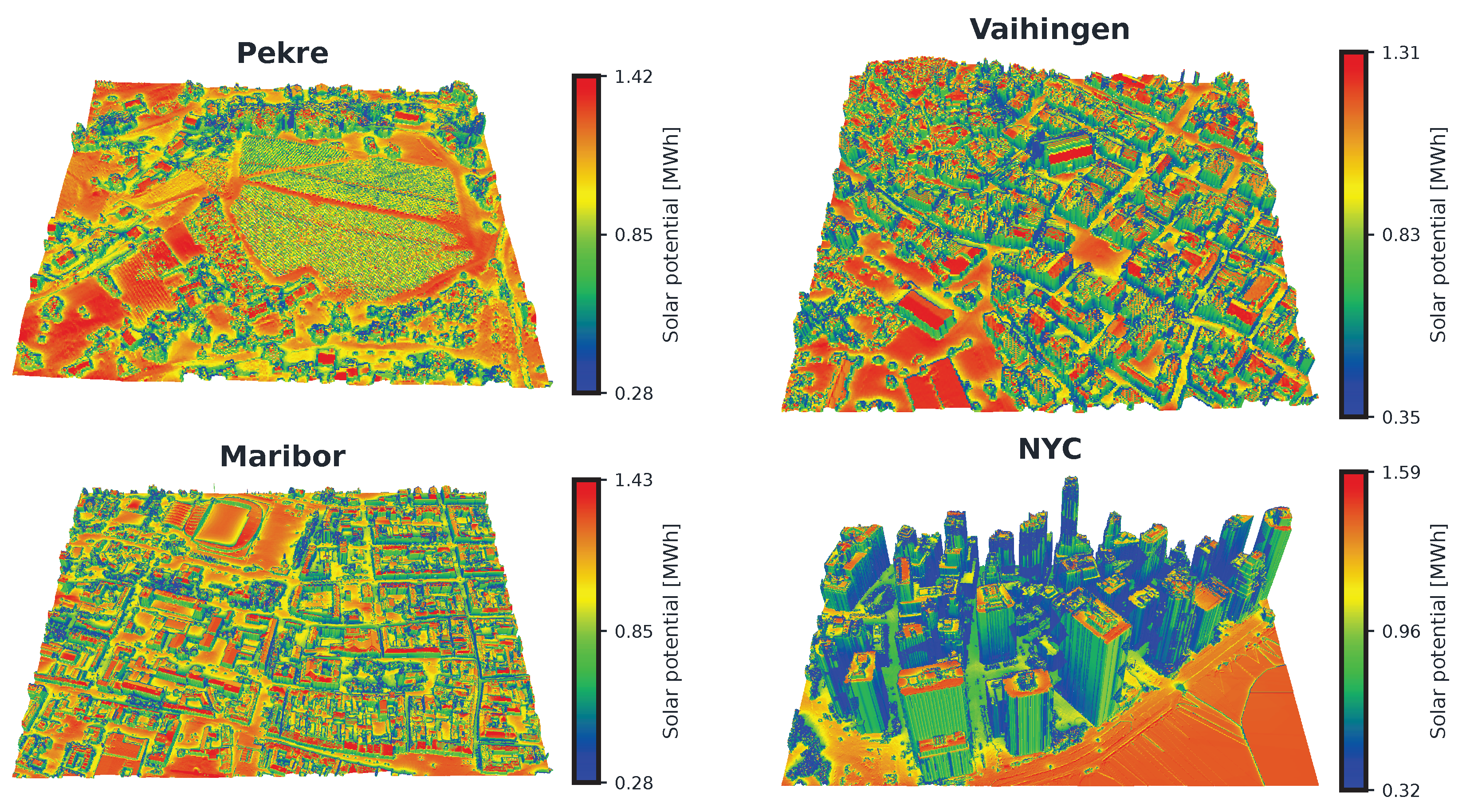
The full pipeline was evaluated additionally on four LiDAR-derived DSMs of contrasting urban morphology: a suburban area in Pekre, Slovenia ( 46.54 N, 15.59 E), a low-rise urban area in Maribor, Slovenia ( 46.55 N, 15.65 E), a low-rise urban area in Vaihingen, Germany ( 48.93 N, 8.96 E), and a dense high-rise area of Lower Manhattan, New York City (NYC) ( 40.70 N, 74.01 W). The DSMs were generated by using only classified LiDAR points and the gaps were filled with inverse distance weighting interpolation. Additional input was the TMY irradiance data for each location, being openly available through the respective national meteorological organisations. It should be noted that these experiments focused strictly on the usability and computational performance, as the physical accuracy of the underlying solar potential estimation had been validated in prior work [33]. All four datasets were voxelised at the same 1 m resolution and processed with the strongest rle_4_8_16_24_32 configuration. Moreover, the uncompressed no_compr pipeline ran on identical inputs as a reference. The four areas differ by building heights, as wall voxels accounted for ≈38% of | V | in Pekre, ≈51% in both Vaihingen and Maribor, and ≈76% in NYC. The results are summarised in Table 3, and the areas’ annual solar potential estimated with the proposed method is visualised in Figure 13.
Pekre attained the lowest CR of the four sites ( CR = 2.95 ), because its open suburban morphology produces the most fragmented viewsheds, and ba_RLE compresses fragmented viewsheds least effectively. Over a low, open skyline the occluders that a voxel does see are few and widely scattered, so the descending index sequence yields large and irregular deltas that change the bit-width group frequently. These frequent transitions shorten the same-group runs, which increases the number of tokens and EOV guards relative to the encoded delta payload. Moreover, since each run is byte-aligned, the padding of short runs takes a larger fraction of the binary stream. In the deep urban canyons of NYC, by contrast, each voxel is surrounded by mutually occluding facades at short range, so most rays terminate on a small number of nearby voxels. The resulting indices are clustered densely, the deltas are correspondingly small and uniform, and long runs within the same bit-width group are formed, which explains the highest observed ratio ( CR = 3.40 ). Maribor and Vaihingen, with their intermediate mixed low- and mid-rise morphology, fall between the two ( CR = 3.30 and 3.21 ).

4. Conclusions

This paper presented a GPU-accelerated method for estimating solar irradiance over Digital Surface Models (DSMs) that, beyond direct and diffuse irradiance and shadowing, also accounts for first- and second-order surface inter-reflection. A novel structurally lossless set-based compression scheme was proposed to keep the per-voxel viewshed information that reflection requires within the GPU memory budget. It is built on a bit-aware Run-Length Encoding (ba_RLE) of delta-coded visibility indices together with a byte-aligned, GPU-friendly binarisation, i.e., a domain-specific compression of remote sensing-derived visibility data that preserves exactly the visibility structure consumed by the radiative model, rather than a general-purpose integer coder. An ablation analysis over eight synthetic DSMs spanning an order of magnitude in voxel count showed that the full rle_4_8_16_24_32 configuration achieved the highest CR (up to 3.3 ).
Some limitations should be noted. First, because compression trades device memory for decompression work, its benefit is conditional on the area scale and morphology: over smaller areas every RLE variant remained slower than the uncompressed baseline, and the runtime gap only narrowed as | V | grew. Second, over sparse or near-flat terrain, where few vertical voxels are present and the reflective component is small, the use of compression yields limited practical return. Third, compression is currently performed once on the host, leaving a host-side preprocessing bottleneck that the present work does not address. Fourth, the bit-width group boundaries are fixed a priori and are not adapted to the local visibility statistics, so a dataset whose delta distribution falls near a bin edge cannot exploit the binning as effectively as the reported results suggest. Fifth, the compressed viewshed is bound to a static scene, since any geometric change, e.g., new construction or seasonal vegetation growth, invalidates the affected per-voxel streams and requires repeating the host-side preprocessing. Sixth, the observed behaviour beyond the device memory budget depends on the driver’s shared system memory fallback, which is vendor- and operating-system-specific, so the exact scale at which compression becomes enabling varies with the hardware. Lastly, the underlying radiative model retains its simplifying assumptions, namely a constant Lambertian diffuse albedo with no specular component. In addition, the viewshed is sampled at a fixed angular resolution | P | , to which both the accuracy of the reflective term and the attainable compression are tied.
Beyond the solar potential estimation, the core idea, compressing the per-voxel viewshed once and streaming it through the GPU kernel on demand, is applicable to any simulation in which the same visibility information is consumed repeatedly over many time steps. A natural extension is longwave thermal irradiance, where estimating the radiative exchange between a surface and its surroundings (and the sky) requires, for each voxel, exactly the set of surfaces visible from it. It is weighted by the same geometric form factors already computed in this paper. Furthermore, the same reuse pattern benefits sky-view-factor and longwave-trapping analyses in urban-heat-island applications. Finally, the proposed method could also be relevant to dynamic line-of-sight and visibility applications that recur across time, such as hourly glare or reflection-hazard assessment from facades, as well as dynamic signal propagation or sensor coverage estimation.
On the methodological side, several future research directions follow directly from the stated limitations. The host-side encoding could be ported to the GPU to remove the preprocessing bottleneck. It could be extended further towards incremental re-encoding, whereby a localised geometric change updates only the affected per-voxel streams instead of triggering a full recomputation. The fixed bit-width binning could be made adaptive, by selecting the group boundaries per dataset. Finally, coupling the compressed viewshed streaming with multi-GPU tiling would extend the method towards a regional- or country-scale solar cadastre. An evaluation across different LiDAR spatial resolutions would establish the generality of the reported compression behaviour further.

Author Contributions

N.L., writing—original draft, writing—review and editing, visualisation, validation, software, methodology, investigation, conceptualisation, formal analysis, data curation, project administration. B.Ž., writing—original draft, software, methodology, investigation, conceptualisation, writing—review and editing. All authors have read and agreed to the published version of the manuscript.

Funding

This work was co-funded by the Slovenian Research and Innovation Agency, under the basic research project No. J7-50095, and research programme No. P2-0041.

Data Availability Statement

The full C++ and CUDA based source code of the proposed method is publicly available at: https://github.com/SAMPA-Project/SolarGPU (accessed on 28 August 2026). All datasets used in this paper are publicly available and can be downloaded at https://doi.org/10.5281/zenodo.22145532.

Acknowledgments

The authors gratefully acknowledge Germany’s National Meteorological Service, the Slovenian Environmental Agency, and the National Renewable Energy Laboratory (US) for providing the solar irradiance meteorological measurements. We also extend our gratitude to the German Society for Photogrammetry, Remote Sensing and Geoinformation (DGPF), the Slovenian Environmental Agency, and the State of New York (US) for supplying open LiDAR data.

Conflicts of Interest

The authors declare that they have no known competing financial interests or personal relationships that could have appeared to influence the work reported in this paper.

References

  1. Manapragada, N.V.S.K.; Mandelmilch, M.; Roitberg, E.; Kizel, F.; Natanian, J. Remote sensing for environmentally responsive urban built environment: A review of tools, methods and gaps. Remote Sens. Appl. Soc. Environ. 2025, 38, 101529. [Google Scholar] [CrossRef] [Scilit]
  2. Lukač, N.; Mongus, D.; Žalik, B.; Štumberger, G.; Bizjak, M. Novel GPU-accelerated high-resolution solar potential estimation in urban areas by using a modified diffuse irradiance model. Appl. Energy 2024, 353, 122129. [Google Scholar] [CrossRef] [Scilit]
  3. Jakubiec, J.A.; Reinhart, C.F. A method for predicting city-wide electricity gains from photovoltaic panels based on LiDAR and GIS data combined with hourly Daysim simulations. Sol. Energy 2013, 93, 127–143. [Google Scholar] [CrossRef] [Scilit]
  4. Nouri, B.; Kuhn, P.; Wilbert, S.; Prahl, C.; Pitz-Paal, R.; Blanc, P.; Schmidt, T.; Yasser, Z.; Santigosa, L.R.; Heineman, D. Nowcasting of DNI maps for the solar field based on voxel carving and individual 3D cloud objects from all sky images. AIP Conf. Proc. 2018, 2033, 190011. [Google Scholar] [CrossRef] [Scilit]
  5. Hoang, A.T.; Pham, V.V.; Nguyen, X.P. Integrating renewable sources into energy system for smart city as a sagacious strategy towards clean and sustainable process. J. Clean. Prod. 2021, 305, 127161. [Google Scholar] [CrossRef] [Scilit]
  6. Lukač, N.; Seme, S.; Sredenšek, K.; Štumberger, G.; Mongus, D.; Žalik, B.; Bizjak, M. Detection and Optimization of Photovoltaic Arrays’ Tilt Angles Using Remote Sensing Data. Appl. Sci. 2025, 15, 3598. [Google Scholar] [CrossRef] [Scilit]
  7. Bizjak, M.; Žalik, B.; Štumberger, G.; Lukač, N. Large-scale estimation of buildings’ thermal load using LiDAR data. Energy Build. 2021, 231, 110626. [Google Scholar] [CrossRef] [Scilit]
  8. Yuan, J.; Yan, D.; Xiao, X.; Shimazaki, Y.; Wang, Y.; Jiao, Z.; Lin, Z.; Bizjak, M.; Farnham, C.; Emura, K. Mitigating urban heat islands: Enhancing outdoor comfort with retro-reflective building materials through computational-fluid-dynamics analysis. Next Res. 2025, 2, 100199. [Google Scholar] [CrossRef] [Scilit]
  9. Arias-Rosales, A.; LeDuc, P.R. Urban solar harvesting: The importance of diffuse shadows in complex environments. Renew. Sustain. Energy Rev. 2023, 175, 113155. [Google Scholar] [CrossRef] [Scilit]
  10. Huang, Y.; Chen, Z.; Wu, B.; Chen, L.; Mao, W.; Zhao, F.; Wu, J.; Wu, J.; Yu, B. Estimating Roof Solar Energy Potential in the Downtown Area Using a GPU-Accelerated Solar Radiation Model and Airborne LiDAR Data. Remote Sens. 2015, 7, 17212–17233. [Google Scholar] [CrossRef] [Scilit]
  11. Kaynak, S.; Kaynak, B.; Özmen, A. GPU-Based Dynamic Solar Potential Estimation Tool Using 3D Plans. IEEE Access 2020, 8, 45432–45442. [Google Scholar] [CrossRef] [Scilit]
  12. Laine, S.; Karras, T. Efficient sparse voxel octrees. In Proceedings of the 2010 ACM SIGGRAPH Symposium on Interactive 3D Graphics and Games (I3D ’10), Washington, DC, USA, 19–21 February 2010; pp. 55–63. [Google Scholar] [CrossRef] [Scilit]
  13. Liang, J.; Gong, J. A Sparse Voxel Octree-Based Framework for Computing Solar Radiation Using 3D City Models. ISPRS Int. J. Geo-Inf. 2017, 6, 106. [Google Scholar] [CrossRef] [Scilit]
  14. Lukač, N.; Mongus, D.; Štumberger, G.; Bizjak, M. GPU-accelerated Sparse Voxel Octree for Irradiance Simulation using Remote Sensing Data. In Proceedings of the 2025 14th International Conference on Renewable Energy Research and Applications (ICRERA); IEEE: Piscataway, NJ, USA, 2025; pp. 665–669. [Google Scholar] [CrossRef] [Scilit]
  15. Shannon, C.E. A mathematical theory of communication. Bell Syst. Tech. J. 1948, 27, 379–423. [Google Scholar] [CrossRef] [Scilit]
  16. Fano, R.M. The Transmission of Information; Technical Report 65; Research Laboratory of Electronics, Massachusetts Institute of Technology: Cambridge, MA, USA, 1949. [Google Scholar]
  17. Huffman, D.A. A Method for the Construction of Minimum-Redundancy Codes. Proc. IRE 1952, 40, 1098–1101. [Google Scholar] [CrossRef] [Scilit]
  18. Salomon, D.; Motta, G. Handbook of Data Compression, 5th ed.; Springer: Berlin/Heidelberg, Germany, 2010. [Google Scholar] [CrossRef] [Scilit]
  19. Bodden, E.; Clasen, M.; Kneis, J. Arithmetic Coding Revealed—A Guided Tour from Theory to Praxis; Technical Report 2007-5; Sable Research Group, School of Computer Science, McGill University: Montreal, QC, Canada, 2007. [Google Scholar]
  20. Duda, J.; Tahboub, K.; Gadgil, N.J.; Delp, E.J. The Use of Asymmetric Numeral Systems as an Accurate Replacement for Huffman Coding. In Proceedings of the 2015 Picture Coding Symposium (PCS); IEEE: Piscataway, NJ, USA, 2015; pp. 65–69. [Google Scholar] [CrossRef] [Scilit]
  21. Ziv, J.; Lempel, A. A Universal Algorithm for Sequential Data Compression. IEEE Trans. Inf. Theory 1977, 23, 337–343. [Google Scholar] [CrossRef] [Scilit]
  22. Golomb, S.W. Run-Length Encodings. IEEE Trans. Inf. Theory 1966, 12, 399–401. [Google Scholar] [CrossRef] [Scilit]
  23. Rice, R.F. Some Practical Universal Noiseless Coding Techniques; Technical Report JPL-PUB-79-22; Jet Propulsion Laboratory, California Institute of Technology: Pasadena, CA, USA, 1979. [Google Scholar]
  24. Sathish, V.; Schulte, M.J.; Kim, N.S. Lossless and lossy memory I/O link compression for improving performance of GPGPU workloads. In Proceedings of the 21st International Conference on Parallel Architectures and Compilation Techniques, Minneapolis, MN, USA, 19–23 September 2012; pp. 325–334. [Google Scholar] [CrossRef] [Scilit]
  25. Shanbhag, A.; Yogatama, B.W.; Yu, X.; Madden, S. Tile-based lightweight integer compression in GPU. In Proceedings of the 2022 International Conference on Management of Data, Philadelphia, PA, USA, 12–17 June 2022; pp. 1390–1403. [Google Scholar] [CrossRef] [Scilit]
  26. Afroozeh, A.; Felius, L.; Boncz, P. Accelerating GPU Data Processing using FastLanes Compression. In Proceedings of the 20th International Workshop on Data Management on New Hardware, Santiago, Chile, 10 June 2024; pp. 1–11. [Google Scholar] [CrossRef] [Scilit]
  27. Mallia, A.; Siedlaczek, M.; Suel, T.; Zahran, M. Gpu-accelerated decoding of integer lists. In Proceedings of the 28th ACM International Conference on Information and Knowledge Management, Beijing, China, 3–7 November 2019; pp. 2193–2196. [Google Scholar]
  28. Gera, P.; Kim, H. Traversing large compressed graphs on GPUs. In Proceedings of the 2023 IEEE International Parallel and Distributed Processing Symposium (IPDPS); IEEE: Piscataway, NJ, USA, 2023; pp. 25–35. [Google Scholar]
  29. Knorr, F.; Thoman, P.; Fahringer, T. Ndzip-gpu: Efficient lossless compression of scientific floating-point data on GPUs. In Proceedings of the International Conference for High Performance Computing, Networking, Storage and Analysis, St. Louis, MI, USA, 14–19 November 2021; pp. 1–14. [Google Scholar] [CrossRef] [Scilit]
  30. Shah, M.; Yu, X.; Di, S.; Becchi, M.; Cappello, F. Lightweight huffman coding for efficient gpu compression. In Proceedings of the 37th International Conference on Supercomputing, Orlando, FL, USA, 21–23 June 2023; pp. 99–110. [Google Scholar] [CrossRef] [Scilit]
  31. Zhang, B.; Tian, J.; Di, S.; Yu, X.; Feng, Y.; Liang, X.; Tao, D.; Cappello, F. Fz-gpu: A fast and high-ratio lossy compressor for scientific computing applications on gpus. In Proceedings of the 32nd International Symposium on High-Performance Parallel and Distributed Computing, Orlando, FL, USA, 20–23 June 2023; pp. 129–142. [Google Scholar] [CrossRef] [Scilit]
  32. Huang, Y.; Di, S.; Li, G.; Cappello, F. CuSZp2: A GPU lossy compressor with extreme throughput and optimized compression ratio. In Proceedings of the SC24: International Conference for High Performance Computing, Networking, Storage and Analysis; IEEE: Piscataway, NJ, USA, 2024; pp. 1–18. [Google Scholar] [CrossRef] [Scilit]
  33. Lukač, N.; Špelič, D.; Štumberger, G.; Žalik, B. Optimisation for large-scale photovoltaic arrays’ placement based on Light Detection And Ranging data. Appl. Energy 2020, 263, 114592. [Google Scholar] [CrossRef] [Scilit]
  34. Duffie, J.A.; Beckman, W.A.; Blair, N. Solar Engineering of Thermal Processes, Photovoltaics and Wind; John Wiley & Sons: Hoboken, NJ, USA, 2020. [Google Scholar] [CrossRef] [Scilit]
  35. Blanco-Muriel, M.; Alarcón-Padilla, D.C.; López-Moratalla, T.; Lara-Coira, M. Computing the solar vector. Sol. Energy 2001, 70, 431–441. [Google Scholar] [CrossRef] [Scilit]
  36. Perez, R.; Ineichen, P.; Seals, R.; Michalsky, J.; Stewart, R. Modeling daylight availability and irradiance components from direct and global irradiance. Sol. Energy 1990, 44, 271–289. [Google Scholar] [CrossRef] [Scilit]
  37. Murray, J.D.; VanRyper, W. Encyclopedia of Graphics File Formats, 2nd ed.; O’Reilly & Associates: Sebastopol, CA, USA, 1996. [Google Scholar]
  38. Žalik, B.; Mongus, D.; Žalik, K.R.; Podgorelec, D.; Lukač, N. Lossless chain code compression with an improved Binary Adaptive Sequential Coding of zero-runs. J. Vis. Commun. Image Represent. 2021, 75, 103050. [Google Scholar] [CrossRef] [Scilit]
  39. Burrows, M.; Wheeler, D.J. A Block–Sorting Lossless Data Compression Algorithm; Technical Report 124; Digital Equipment Corporation, Systems Research Center: Palo Alto, CA, USA, 1994. [Google Scholar]
  40. Žalik, B.; Mongus, D.; Lukač, N.; Žalik, K.R. Can Burrows–Wheeler transform be replaced in chain code compression? Inf. Sci. 2020, 525, 109–118. [Google Scholar] [CrossRef] [Scilit]
  41. Cebecauer, T.; Suri, M. Typical Meteorological Year Data: SolarGIS Approach. Energy Procedia 2015, 69, 1958–1969. [Google Scholar] [CrossRef] [Scilit]
Figure 1. Overview of the proposed method’s pipeline. Data preprocessing and structurally lossless viewshed compression are performed once on the host, where the compressed binary stream is then decompressed on-the-fly on the GPU.
Remotesensing 18 03044 g001
Figure 2. From a DSM to a per-voxel viewshed. (a) Each raster cell z ( x , y ) yields a top-surface voxel, and vertical wall voxels are inserted along the exposed face; (b) For a voxel v, rays are cast over | P | patches of the sphere; (c) Resulting visibility-index vector Ω v = Ω v , i , 0 i < | P | .
Remotesensing 18 03044 g002
Figure 3. An example of determining ba_RLE tokens.
Remotesensing 18 03044 g003
Figure 4. Eight bit-packed groups from the first eight tokens.
Remotesensing 18 03044 g004
Figure 5. Sun-band visibility bitmask and constant-time shadow test. (a) Rays cast once from voxel v determine, per hemisphere patch visibility; (b) Over a year the Sun occupies only a small subset A P ; (c) These bits are packed into per-voxel bitmask M v of N a / 8 bytes.
Remotesensing 18 03044 g005
Figure 6. Per-hour GPU kernel orchestration. For every daylight hour per-voxel accumulators are reset and four kernels run in sequence.
Remotesensing 18 03044 g006
Figure 7. Visualisation of eight synthetic datasets and their estimated annual solar potential with the proposed method.
Remotesensing 18 03044 g007
Figure 8. CR heatmap, where the brighter cells indicate stronger compression.
Remotesensing 18 03044 g008
Figure 9. Absolute GPU memory heatmap in GB.
Remotesensing 18 03044 g009
Figure 10. Total GPU runtime by variant across all datasets.
Remotesensing 18 03044 g010
Figure 11. Decompression-efficiency heatmap based on E metric.
Remotesensing 18 03044 g011
Figure 12. Performance-index heatmap based on Π metric, summarizing joint quality-speed trade-off across all the dataset-variant pairs.
Remotesensing 18 03044 g012
Figure 13. 3D visualisation of four LiDAR derived DSMs and their estimated annual solar potential with the proposed method.
Remotesensing 18 03044 g013
Table 1. Synthetic DSMs used in the ablation analysis, ordered by voxel count.
Dataset W × H [m] | V | Uncompressed Viewshed [MB]Total Time [s]
data1512 × 512381,44542334
data2512 × 512629,177118787
data3512 × 512854,4801840126
data41024 × 10241,358,865125499
data51024 × 10241,652,7112231175
data61024 × 10241,951,8063192240
data72048 × 20488,843,57018,9751356
data82048 × 204811,917,51829,61024,079
Table 2. Deviation between the solar potential obtained with the uncompressed and the compressed viewshed representation. Furthermore, comparison relative to the single-precision epsilon ε 1.19 × 10 7 is provided.
Dataset | V | δ max δ max / ε δ rms
data1381,445 2.71 × 10 7 2.3 1.76 × 10 8
data2629,177 4.19 × 10 7 3.5 2.18 × 10 8
data3854,480 3.27 × 10 7 2.7 2.40 × 10 8
data41,358,865 3.55 × 10 7 3.0 1.69 × 10 8
data51,652,711 3.29 × 10 7 2.8 1.87 × 10 8
data61,951,806 3.55 × 10 7 3.0 2.02 × 10 8
data78,843,570 3.64 × 10 7 3.1 1.63 × 10 8
data811,917,518 3.51 × 10 7 2.9 1.72 × 10 8
Table 3. Real LiDAR-derived DSMs and effect of proposed rle_4_8_16_24_32 viewshed compression against the uncompressed baseline (no_compr).
Dataset W × H [m] | V | CRno_comprrle_4_8_16_24_32
Storage [MB] T tot [s]Storage [MB] T tot [s]E [h−1] Π [GB/s]
Pekre 366 × 320 189,3722.95146.10.6649.52.0551770.205
Maribor 864 × 666 1,170,1363.301518.27.91460.720.505800.238
Vaihingen 333 × 293 198,2303.21209.40.9965.32.7342230.240
NYC 799 × 457 1,522,2753.403351.118.03985.943.772810.254
Disclaimer/Publisher’s Note: The statements, opinions and data contained in all publications are solely those of the individual author(s) and contributor(s) and not of MDPI and/or the editor(s). MDPI and/or the editor(s) disclaim responsibility for any injury to people or property resulting from any ideas, methods, instructions or products referred to in the content.