Trajectory-Guided Photon Accumulation for Photon-Efficient LiDAR Remote Sensing in Low-SBR Dynamic Scenes

Highlights

What are the main findings?

• Range-time guidance aligns and accumulates weak photon returns dispersed by line-of-sight motion.
• Background-corrected multi-scale statistics and cross-scale fusion recover spatial and range information under the tested low-SBR conditions.

What are the implications of the main findings?

• Deterministic range-time migration can serve as a physical constraint for photon-efficient active remote sensing reconstruction.
• The method offers a potential basis for long-range and weak-target observation, subject to further field validation.

Abstract

Photon-efficient LiDAR provides an active remote sensing pathway for long-range, low-light three-dimensional observation, but photon-limited reconstruction remains difficult when background events dominate sparse returns. In dynamic scenes, line-of-sight motion further disperses weak-target photons across range-time bins and broadens fixed-bin accumulation. Existing methods mainly exploit histogram statistics, spatial priors, or learned representations, whereas explicit range-time migration constraints for interframe photon alignment remain insufficiently explored. We present a range-time trajectory-guided photon accumulation method for a 1064 nm InGaAs/InP $64\times 64$ GM-APD array. The method combines range-dependent background correction, multi-scale photon statistics, bounded trajectory parameter optimization using PSO, trajectory-aligned accumulation, and confidence-weighted spatial-range fusion. At -12.34 dB in simulation, SSIM, RMSE (range bins), PSNR, IoU, and FPR were 0.61, 223.22, 6.36 dB, 0.74, and 0.10%, respectively. Across 19 experimentally generated low-SBR evaluation cases derived from measured GM-APD LiDAR sequences, the corresponding mean values were $0.541\pm 0.165$, $332.93\pm 79.60$, $8.60\pm 2.49$ dB, $0.702\pm 0.061$, and $0.33\pm 0.08$%. Under the tested conditions, range-time guidance preserved spatial structure and pixel-wise range information while suppressing background responses, supporting photon-limited reconstruction in active remote sensing.

1. Introduction

Photon-counting LiDAR is an active remote sensing modality that combines time-resolved ranging with sensitivity to very weak optical returns. Its single-photon detection capability supports long-range observation, low-light imaging, weak-target observation, and airborne sensing configurations in which conventional intensity measurements may provide insufficient return energy. Geiger-mode avalanche photodiode (GM-APD) arrays extend this capability through parallel spatial acquisition and have enabled near-infrared three-dimensional imaging and few-photon target observation with array detectors [1,2,3]. A 1064 nm InGaAs/InP array is particularly relevant to the present study because it combines near-infrared sensitivity, gated acquisition, and pixel-wise time-of-flight measurement. Unlike a conventional grayscale imager, however, such an array records discrete photon-trigger events whose distribution depends on temporal quantization, detector response, and observation conditions [4].

Photon-counting LiDAR has become an important active remote sensing technique for long-range and low-light three-dimensional observation. Airborne single-photon systems and the MABEL/ICESat-2 development path demonstrate the capability to retrieve weak optical returns under photon-limited conditions [5,6,7,8]. However, dynamic observation scenarios remain challenging because limited photon returns are further dispersed by motion-induced range migration.

Photon-efficient LiDAR remote sensing becomes difficult when the target return is weak relative to background illumination and detector noise. Background photons, dark counts, and spurious system detections compete with target photons within the acquisition gate. Synchronously gated pixels generally retain only the first valid event, so first-photon competition, dead time, and photon pile-up influence the recorded distribution [9,10,11]. At high background or high flux, these effects reduce the fraction of valid target events available for range recovery [12,13]. Consequently, low signal-to-background ratio (SBR) data must be interpreted at the photon-event level rather than treated as a conventional noisy intensity image.

Dynamic remote sensing observations introduce an additional range-domain degradation. Image-plane displacement mainly changes the spatial location of a weak target, whereas line-of-sight motion changes its interframe time of flight and range-bin position. The resulting photon dispersion spreads returns from the same surface across multiple range bins in the range-time domain. Fixed-bin multiframe accumulation then broadens and weakens the range response and may fragment the recovered spatial structure. Previous studies of moving-scene three-dimensional imaging, high-speed GM-APD reconstruction, dynamic-feature extraction, and field observation have established the importance of temporal continuity in photon-counting data [14,15,16,17]. Area-array GM-APD experiments have also demonstrated dynamic weak-target observation and range-supported UAV imaging [3,18]. For photon-efficient active remote sensing, the central problem is the recovery of three-dimensional information after motion has dispersed scarce photons across range and time. Motion estimation is therefore an intermediate reconstruction constraint rather than the final observation task.

Existing single-photon reconstruction approaches can be grouped into three broad categories. First-photon, waveform-peak, and statistical methods estimate arrival times directly, but may be sensitive to background peaks when valid events are sparse [19,20]. Bayesian and optimization-based reconstruction methods introduce target-presence, background, spatial-neighborhood, nonlocal, or point-cloud priors to improve stability [21,22,23,24,25]. Deep-learning reconstruction methods learn complex spatial and temporal mappings, although their performance depends on agreement between training data and the actual detector response [26]. Existing methods mainly exploit histogram statistics, spatial priors, or learned representations, whereas explicit range-time migration constraints for interframe photon alignment remain insufficiently explored.

The comparison methods used in this work represent distinct information-use strategies. MDSFF combines multidomain stable features with multi-scale pixel completion, CASPI performs collaborative photon processing, FSPU estimates range from the first signal photon unit, and SPIRAL applies sparse Poisson inversion [27,28,29,30]. These methods provide useful references for spatial feature fusion, collaborative processing, first-event selection, and sparse inversion. In dynamic low-SBR observations, however, interframe changes in echo time of flight create a structured migration path. Explicitly estimating that path provides an opportunity to align dispersed events before accumulation and subsequent range recovery.

This study develops a range-time trajectory-guided photon accumulation method for photon-efficient LiDAR remote sensing in low-SBR dynamic scenes. Full-field multiframe statistics estimate a range-dependent background probability. Background-corrected multi-scale local statistics suppress nonuniform detections while preserving weak-event stability and spatial localization. Candidate range-time paths are described by their range-bin drift rate, initial range position, and trajectory-band width. Bounded trajectory parameter optimization using PSO estimates these parameters. Photon events are then aligned and accumulated along the recovered path. Cross-scale response clustering and confidence-weighted fusion determine the weak-target range interval and candidate spatial region. The final outputs are the reconstructed mask, pixel-wise range values, and confidence map.

The principal contributions are as follows:

• A photon-efficient range-time migration model is developed for dynamic LiDAR remote sensing, linking line-of-sight motion to the interframe dispersion of weak optical returns.
• Background-corrected multi-scale photon statistics are developed to enhance weak returns while balancing spatial localization, photon availability, and suppression of range-dependent background events.
• A trajectory-constrained photon accumulation and cross-scale fusion strategy is developed to recover the weak-target range interval, spatial region, pixel-wise range information, and reconstruction confidence in low-SBR dynamic scenes.

2. Photon Observation and Motion-Induced Range Migration in Photon-Counting LiDAR

2.1. Synchronous Gated Single-Photon Observation

Let $p=(x,y)$ denote a spatial pixel, m the frame index, and ℓ the range-bin index. Let ${\lambda }_{t,p}$, ${\lambda }_{b,p}$, and ${\lambda }_{d,p}$ denote the target-return, background, and dark-count intensities. Their sum gives the total latent photon-arrival intensity ${\lambda }_p$:

$${\lambda }_p(\ell ,m)={\lambda }_{t,p}(\ell ,m)+{\lambda }_{b,p}(\ell ,m)+{\lambda }_{d,p}(\ell ,m)$$

(1)

At low flux, an inhomogeneous Poisson point process describes the latent incident events [9]. The observation sequence $\mathbf{D}(p,m)$, however, stores at most one valid range bin for each pixel and frame. This single-timestamp readout follows a discrete first-event detection model, so records in different range bins are not independent Poisson counts. Let r denote a range-bin index preceding ℓ. The explicit first-event probability of recording bin ℓ is

$$Pr[\mathbf{D}(p,m)=\ell ]=exp\left[-\sum _{r<\ell }{\lambda }_p(r,m)\right]\left\{1-exp[-{\lambda }_p(\ell ,m)]\right\}$$

(2)

The survival probability from gate opening through bin $\ell -1$ is denoted by $q_{p,\ell ,m}$:

$$q_{p,\ell ,m}=exp\left\{-\sum _{r<\ell }{\lambda }_p(r,m)\right\}$$

(3)

The remaining probability corresponds to no valid record within the acquisition gate. Equations (2) and (3) describe first-event competition, in which an earlier background event or dark count can prevent a later target return from being recorded. This mechanism produces photon pile-up bias at high flux [10]. The method does not invert the absolute incident intensity. Instead, it constructs empirical histograms from multiframe single-event tags. Subsequent background modeling and photon accumulation therefore operate on the observed event distribution. Detection efficiency and dark counts also affect the effective SBR in gated Geiger-mode detection.

$${\lambda }_{t,p}(\ell ,m)\ll {\lambda }_{b,p}(\ell ,m)+{\lambda }_{d,p}(\ell ,m)$$

(4)

Equation (4) represents a low-SBR condition in which target-arrival intensity is much lower than the combined background and dark-count intensities. Neither the largest single-frame response nor the global range peak can then localize the target reliably. Interframe range continuity and spatial continuity across neighboring pixels help distinguish target from background events.

2.2. Motion-Induced Range Migration in Active Remote Sensing

Let the target range along the line of sight be $R\left(m\right)$. Let $R_0$ denote the initial range, $v_r$ the line-of-sight velocity, and $\mathrm{\Delta }T$ the interframe interval. Under a local constant-velocity approximation, the range in frame m is

$$R\left(m\right)=R_0+v_{r}m\mathrm{\Delta }T$$

(5)

Let ${\ell }_{\mathrm{tar}}\left(m\right)$ denote the target range-bin location and ${\ell }_0$ its initial value. Let c denote the speed of light and $\mathrm{\Delta }\tau$ the time-bin width. The range-bin drift rate is denoted by $\alpha$. The monostatic round-trip time maps continuous range to a discrete range bin:

$${\ell }_{\mathrm{tar}}\left(m\right)={\ell }_0+\alpha m$$

(6)

$$\alpha ={\displaystyle \frac{2v_r\mathrm{\Delta }T}{c\mathrm{\Delta }\tau }}$$

(7)

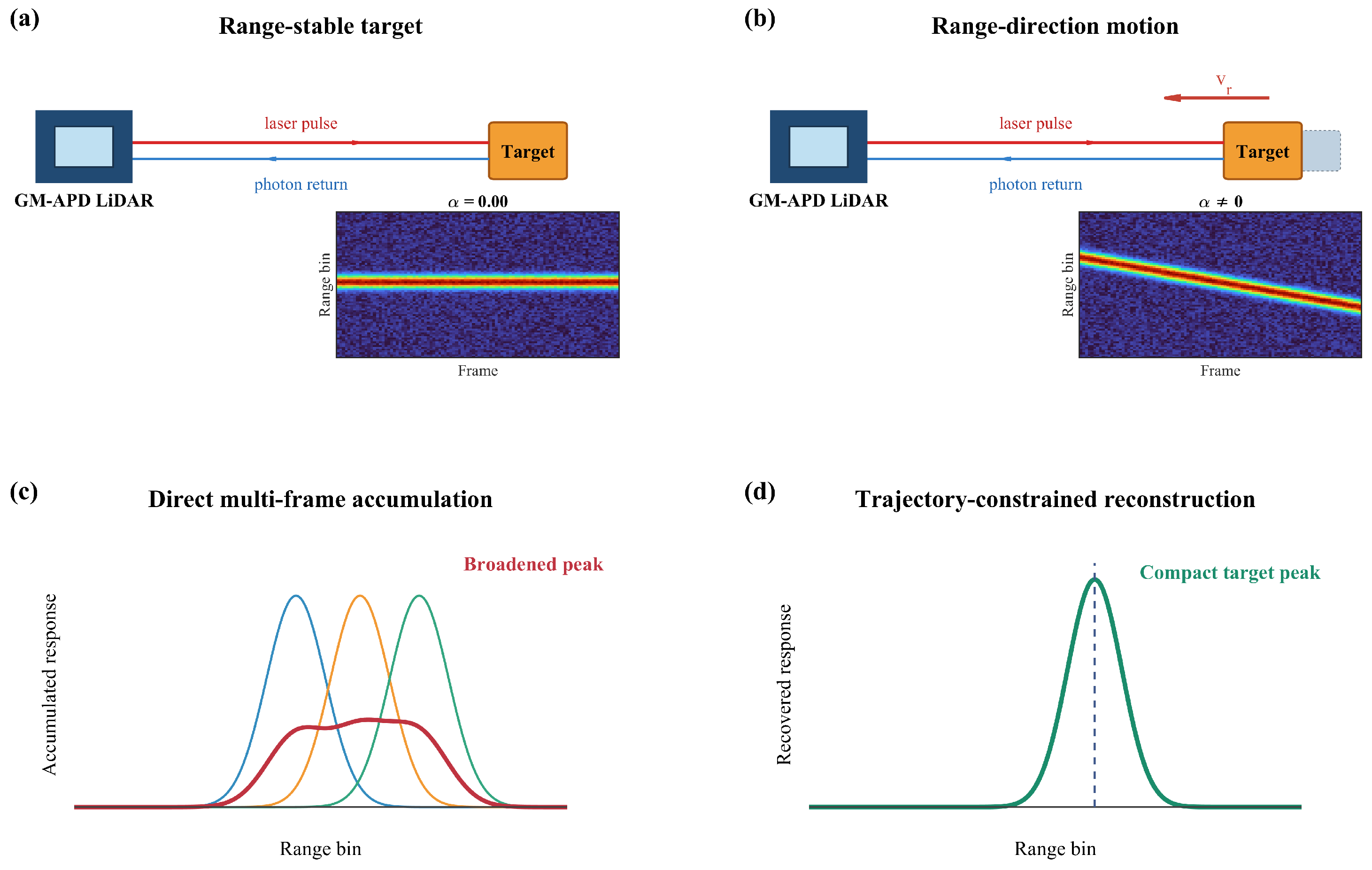
The drift rate $\alpha$ is determined by line-of-sight velocity. For $\alpha \approx 0$, the target range is nearly stable and the photon events form an approximately horizontal band in the range-time domain. For $\alpha \ne 0$, line-of-sight motion shifts the echo across range bins and forms an inclined migration path. The sign of $\alpha$ indicates whether the target recedes or approaches. Weak returns from the same surface are consequently distributed across several range bins over consecutive frames. Fixed-bin multiframe accumulation ignores this displacement, broadens the range peak, and reduces its amplitude [15].

Figure 1 illustrates the difference between direct fixed-bin accumulation and trajectory-constrained reconstruction under range migration.

2.3. Trajectory-Guided Photon Accumulation

Line-of-sight motion shifts the echo across range bins, and the range migration equation describes this displacement in the range-time domain. Under low-SBR conditions, a single-frame weak-target response can fall below background fluctuations. Interframe events must therefore be aligned and accumulated along candidate migration paths. The accumulated response must also exceed the expected background-trigger level. Let $\alpha$ denote the range-bin drift rate, $\beta$ the initial range position, and $\delta$ the trajectory-band half-width. The three-parameter trajectory model is

$$\mathit{\theta }=[\alpha ,\beta ,\delta ]$$

(8)

Here, $\alpha$ is the range-bin drift rate in range bins per frame. Its magnitude describes the rate of range migration, and its sign indicates the direction of line-of-sight motion. The parameter $\beta$ is the target range-bin position at the reference frame $m=0$. The parameter $\delta$ is the half-width of the trajectory band. It provides tolerance for the finite pulse and system-response width, range-bin quantization, and small deviations from the local linear-motion model. For the observed data $\mathbf{D}$, let $L_{\mathrm{photon}}\left(\mathit{\theta }\right)$ denote the accumulated in-band response relative to the expected background. Let $P_{\mathrm{motion}}\left(\mathit{\theta }\right)$ and $P_{\mathrm{space}}\left(\mathit{\theta }\right)$ denote interframe and spatial continuity, respectively. Their weighting coefficients are ${\gamma }_m$ and ${\gamma }_s$. The log-domain trajectory score is

$$E(\mathit{\theta }\mid \mathbf{D})=L_{\mathrm{photon}}\left(\mathit{\theta }\right)+{\gamma }_m{P}_{\mathrm{motion}}\left(\mathit{\theta }\right)+{\gamma }_s{P}_{\mathrm{space}}\left(\mathit{\theta }\right)$$

(9)

The quantity $E(\mathit{\theta }\mid \mathbf{D})$ is the unnormalized trajectory score. The normalized score enables comparison among candidate migration paths. The maximizing parameter vector is denoted by $\widehat{\mathit{\theta }}$:

$$\widehat{\mathit{\theta }}=\underset{\mathit{\theta }}{\arg \max }E(\mathit{\theta }\mid \mathbf{D})$$

(10)

Equations (8)–(10) define the trajectory score under a band-shaped constraint and formulate trajectory estimation as a bounded parameter search. Equation (9) compares the confidence of candidate migration paths. The estimated trajectory parameters then guide the alignment and accumulation of weak-target returns across frames.

2.4. Photon Accumulation Under Range Migration

An isolated background detection can produce a high local response but rarely maintains consistent range migration, side-band contrast, and spatial continuity over many frames. Weak-target events may be sparse in individual frames, yet their accumulated response can exceed the background when they persist along a feasible migration path. Cross-scale consistency further suppresses random background responses. These statistics support trajectory estimation, migration-path clustering, and candidate-region recovery.

Image-plane motion mainly changes the target-pixel position, whereas line-of-sight motion changes the time of flight and range-peak position [14,16,17]. Multi-scale local windows can accommodate limited transverse displacement. The estimated range-bin drift rate describes only range migration caused by line-of-sight motion, not complete two-dimensional or six-degree-of-freedom motion.

3. Photon-Efficient LiDAR Remote Sensing Reconstruction Using Range-Time Trajectory Guidance

3.1. Background-Corrected Multi-Scale Photon Statistics

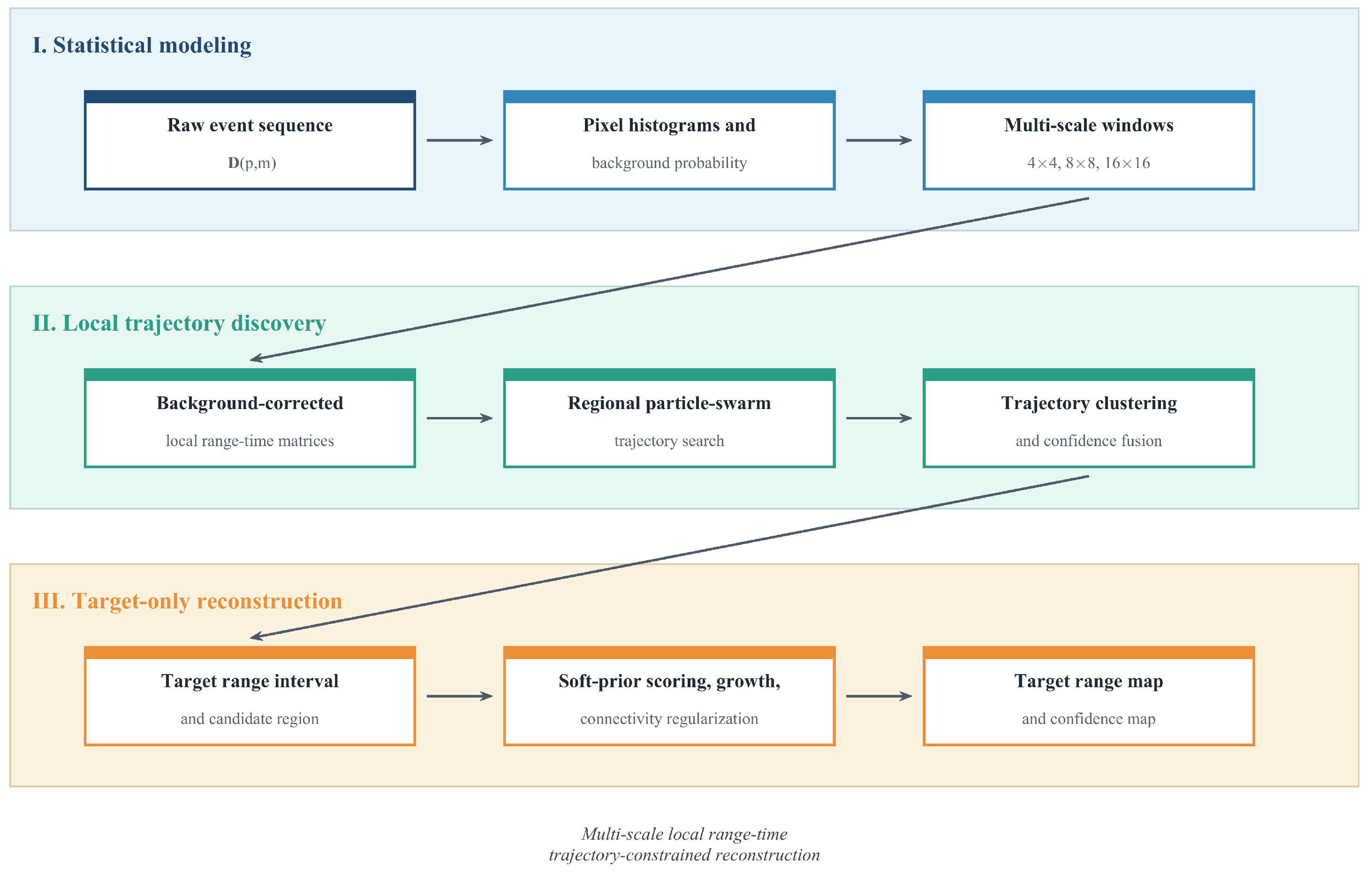
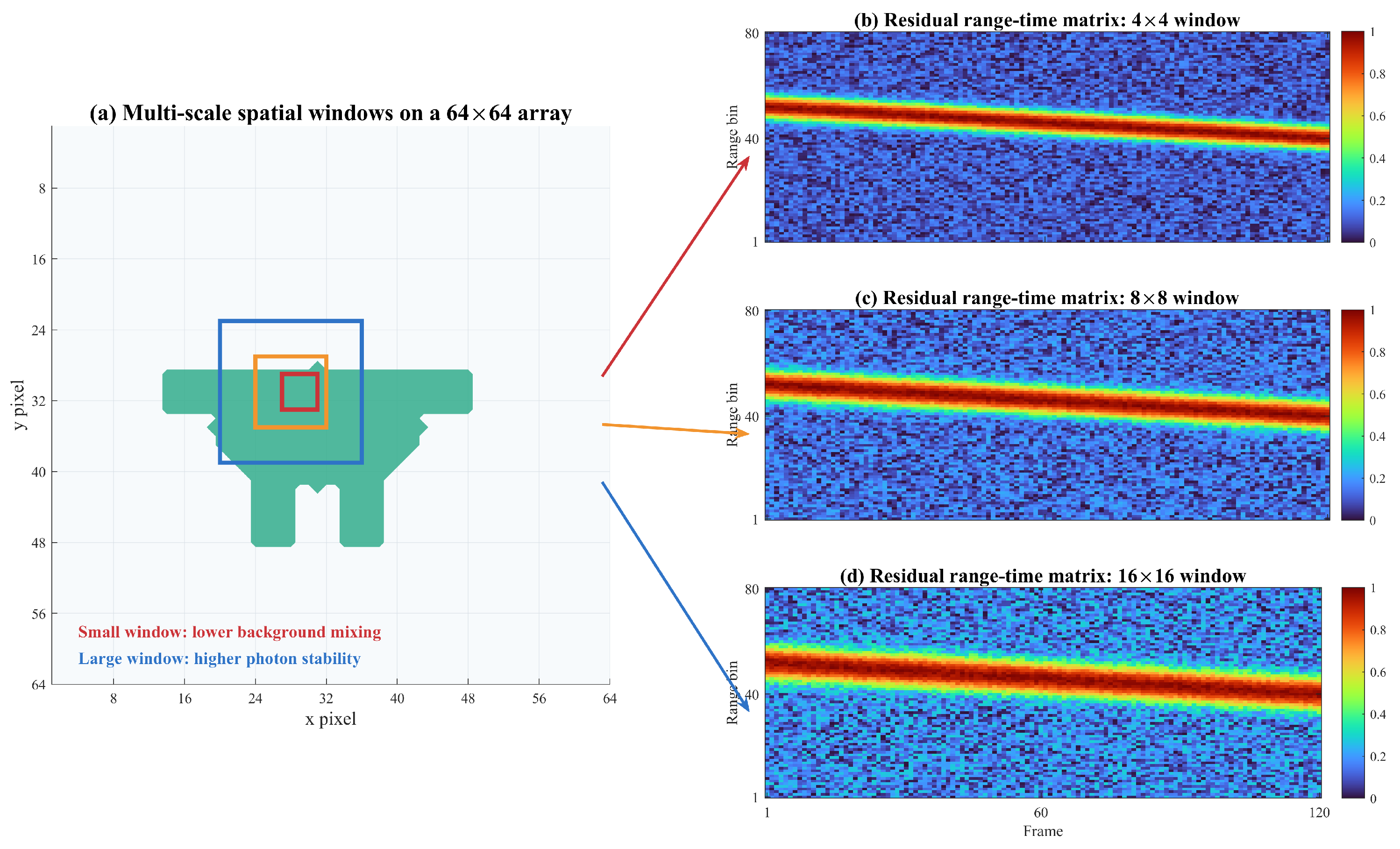
Figure 2 outlines the reconstruction workflow. Full-field multiframe events estimate the range-dependent background probability and generate background-corrected multi-scale local range-time statistics. Sliding windows of 4 × 4, 8 × 8, and 16 × 16 pixels span complementary spatial scales. Small windows limit unrelated background contamination and improve spatial localization. Large windows increase valid event counts and stabilize weak-target responses. Medium windows offer a compromise between target-structure preservation and photon-statistical reliability. A range-time trajectory is estimated within each local window, and weak-target events are accumulated along it. Similar responses across windows and scales are clustered and combined using confidence weights. The fused responses determine the range interval and candidate region. The range map, reconstruction mask, and confidence map are then recovered.

The pixel-wise range histogram is defined as

$$H_p(\ell )=\sum _m\mathrm{I}[\mathbf{D}(p,m)=\ell ]$$

(11)

where $\mathrm{I}[·]$ is the indicator operator. The global background probability is obtained by normalizing the range-event statistics over all pixels:

$$P_{\mathrm{bg}}(\ell )={\displaystyle \frac{{\sum }_p{H}_p(\ell )}{{\sum }_{\ell }{\sum }_p{H}_p(\ell )}}$$

(12)

This probability represents the empirical range distribution of background light, dark counts, and spurious system detections. Within each local window, it determines the expected background-event count for every frame and range bin. Accumulation can therefore emphasize responses that exceed the background level and evolve continuously across frames.

Multi-scale local statistics exploit complementary spatial scales. Small windows limit unrelated background contamination and improve localization, whereas large windows increase valid event counts and stabilize weak-target responses. Consistency across scales suppresses random background responses.

At scale s, let i denote local window ${\mathrm{\Omega }}_i^{\left(s\right)}$. The event count within this window at frame m and range bin ℓ is

$$N_i^{\left(s\right)}(\ell ,m)=\sum _{p\in {\mathrm{\Omega }}_i^{\left(s\right)}}\mathrm{I}[\mathbf{D}(p,m)=\ell ]$$

(13)

For frame m, let $N_i^{\left(s\right)}\left(m\right)$ denote the total valid event count in the window. Under the global background probability, the corresponding expected background-event count is

$$E_i^{\left(s\right)}(\ell ,m)=N_i^{\left(s\right)}\left(m\right)P_{\mathrm{bg}}(\ell )$$

(14)

The local background-corrected range-time matrix is defined as

$${\tilde{T}}_i^{\left(s\right)}(\ell ,m)=max\left\{N_i^{\left(s\right)}(\ell ,m)-E_i^{\left(s\right)}(\ell ,m),0\right\}$$

(15)

The 4 × 4 windows limit unrelated background and improve localization. The 16 × 16 windows increase valid event counts and stabilize weak-target responses. The 8 × 8 windows offer a compromise between target-structure preservation and photon-statistical reliability. After background subtraction, logarithmic compression, two-dimensional smoothing, and normalization, the local matrices support trajectory estimation, migration-path clustering, and target-region fusion.

Continuous high-response bands in the background-corrected local range-time matrices represent target range migration. $\alpha \approx 0$ denotes an approximately stable range, whereas $\alpha \ne 0$ denotes range migration caused by line-of-sight motion. $\beta$ is the initial range position, and $\delta$ is the trajectory-band half-width. The half-width accounts for pulse and system-response broadening, range-bin quantization, and small deviations from the local linear-motion model. Weak-target events can then be aligned and accumulated along the estimated range-time trajectory.

Figure 3 shows the multi-scale spatial windows and their corresponding background-corrected range-time matrices.

3.2. Range-Time Migration Estimation and Trajectory-Guided Accumulation

Within each local background-corrected matrix, a linear range-time trajectory models the target return:

$${\ell }_{\mathit{\theta }}\left(m\right)=\alpha m+\beta ,\mathit{\theta }=[\alpha ,\beta ,\delta ]$$

(16)

The associated trajectory band is

$$B_{\mathit{\theta }}=\{(\ell ,m):|\ell -{\ell }_{\mathit{\theta }}\left(m\right)|\le \delta \}$$

(17)

The trajectory score combines the accumulated in-band response, side-band contrast, temporal coverage, and spatial continuity. Let $E_{\mathrm{track}}$ denote the accumulated response within the trajectory band and $C_{\mathrm{side}}$ the contrast with two flanking background bands. Let $C_{\mathrm{cov}}$ and $C_{\mathrm{spa}}$ denote temporal coverage and spatial continuity. The terms $P_{\mathrm{width}}$ and $P_{\mathrm{slope}}$ penalize excessive width and abnormal slope, and $w_1,\dots ,w_6$ are their fixed score weights. Equation (9) gives the general trajectory-score formulation, whereas Equation (18) is its practical implementation in the PSO optimization. The photon-evidence term $L_{\mathrm{photon}}$ is implemented by the in-band response $E_{\mathrm{track}}$ and side-band contrast $C_{\mathrm{side}}$. The interframe term $P_{\mathrm{motion}}$ is implemented by the positive temporal-coverage term $C_{\mathrm{cov}}$ together with the negative abnormal-slope penalty $P_{\mathrm{slope}}$. The spatial term $P_{\mathrm{space}}$ is implemented by $C_{\mathrm{spa}}$. The additional penalty $P_{\mathrm{width}}$ prevents an excessively wide trajectory band from increasing the accumulated response without physical support. The objective function is

$$E_i^{\left(s\right)}\left(\mathit{\theta }\right)=w_1{E}_{\mathrm{track}}+w_2{C}_{\mathrm{side}}+w_3{C}_{\mathrm{cov}}+w_4{C}_{\mathrm{spa}}-w_5{P}_{\mathrm{width}}-w_6{P}_{\mathrm{slope}}$$

(18)

The PSO bounds are observation-specific rather than universal constants. Let $v_{min}$ and $v_{max}$ denote the expected line-of-sight velocity bounds, and let ${\ell }_{min}$ and ${\ell }_{max}$ denote the valid range-bin interval of the local range-time matrix. Equation (7) gives $\alpha \in [2v_{min}\mathrm{\Delta }T/\left(c\mathrm{\Delta }\tau \right),2v_{max}\mathrm{\Delta }T/\left(c\mathrm{\Delta }\tau \right)]$. For each candidate half-width, the intercept is restricted to $\beta \in [{\ell }_{min}+\delta ,{\ell }_{max}-\delta ]$, so the trajectory band remains inside the observation interval. The bounds ${\delta }_{min}$ and ${\delta }_{max}$ are set from the effective pulse and system-response width, range-bin resolution, and the admissible tolerance for small departures from the local linear-motion model. Bounded trajectory parameter optimization using PSO searches only this three-parameter space [31]. The trajectory-score components were normalized before optimization, and the weights were fixed after scale normalization to avoid domination by any single term.

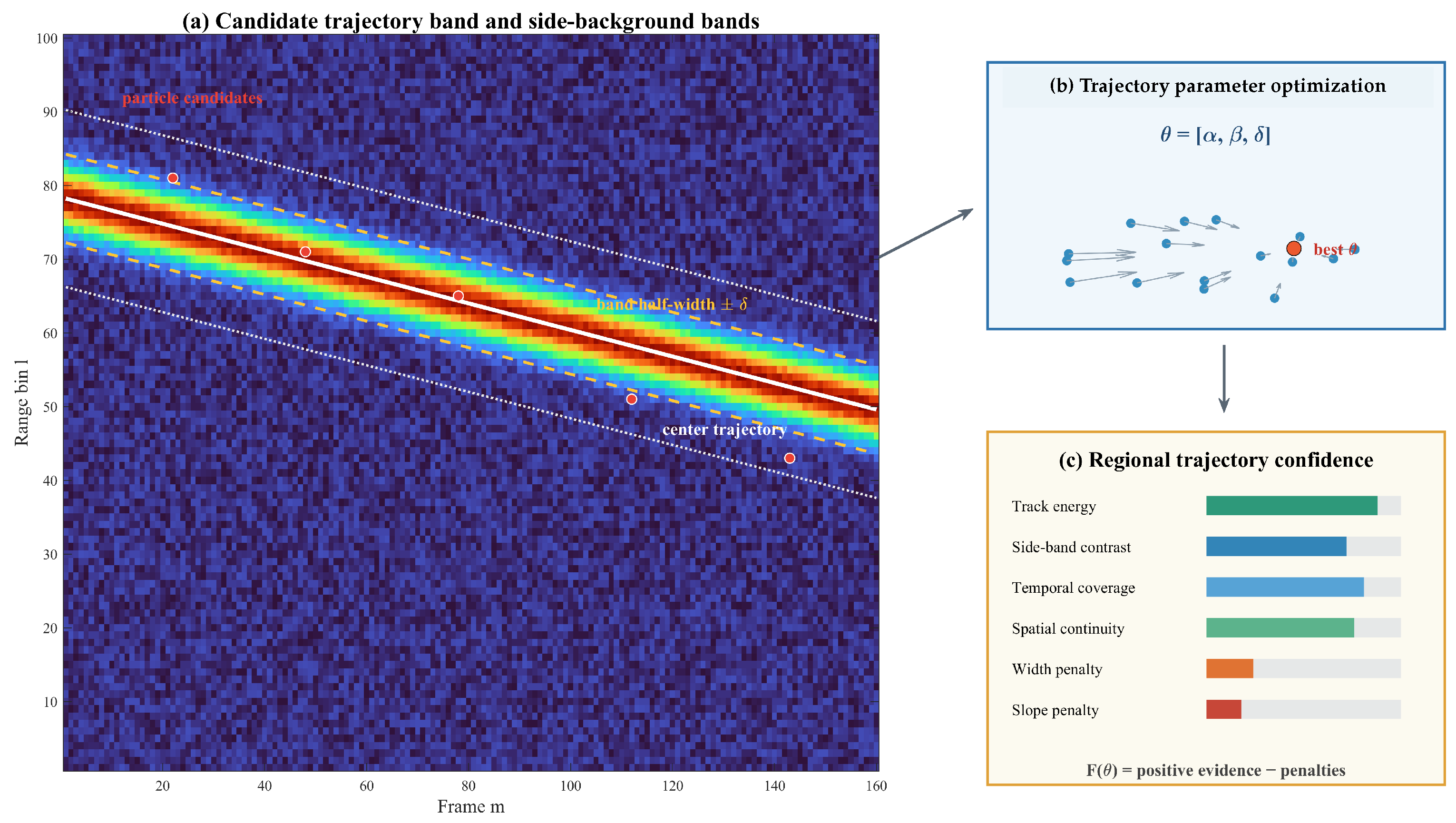
Figure 4 summarizes the trajectory-band construction, bounded PSO search, and regional trajectory-score components.

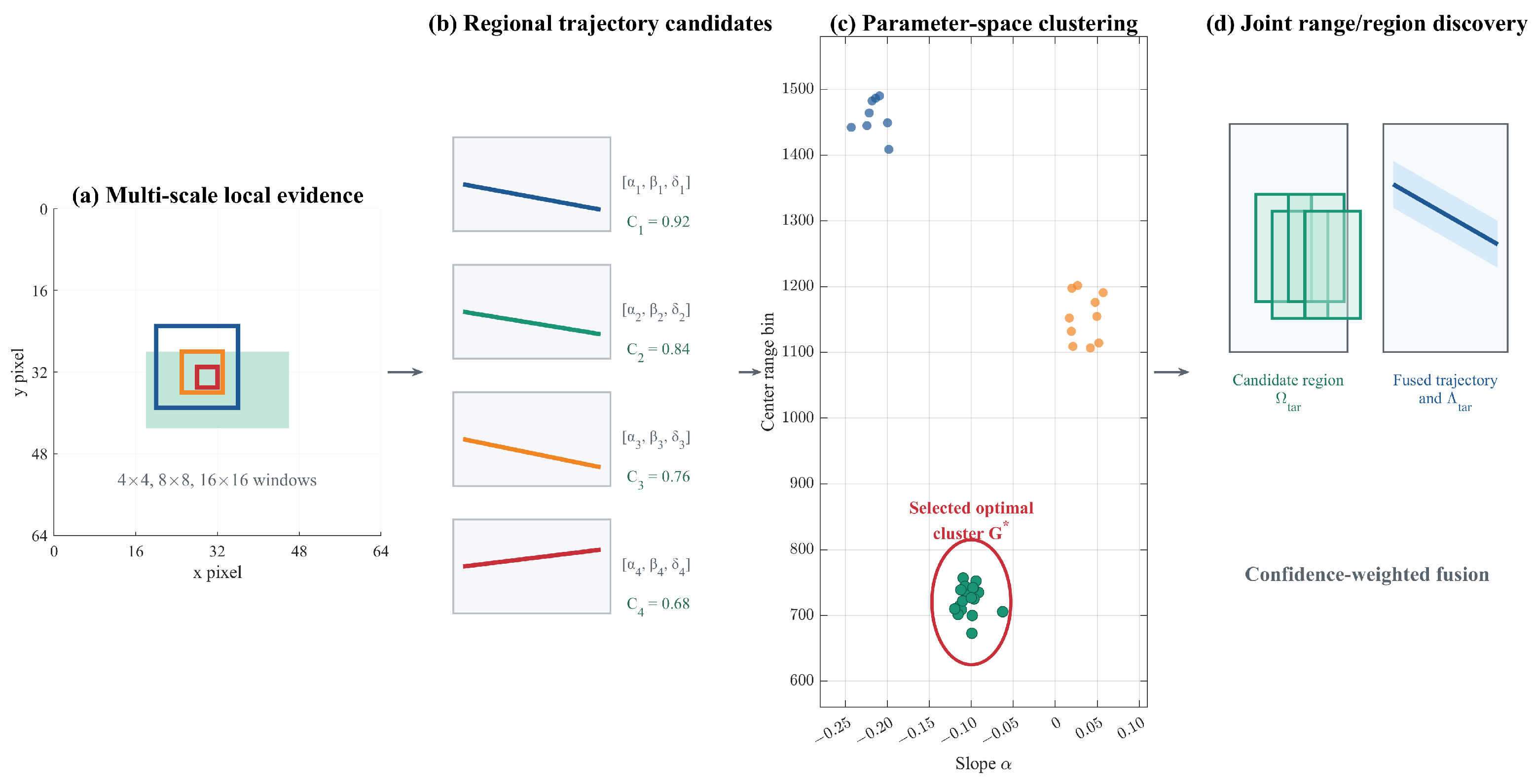
Trajectory candidates are first estimated independently for all local windows at the 4 × 4, 8 × 8, and 16 × 16 spatial scales. Each candidate yields parameters ${\mathit{\theta }}_i^{\left(s\right)}=[{\alpha }_i,{\beta }_i,{\delta }_i]$ and regional confidence score $C_i^{\left(s\right)}$. Candidates from all three scales are then pooled and clustered according to similarity in drift rate $\alpha$, range intercept $\beta$, and band half-width $\delta$. The cluster $G^{*}$ with the highest aggregate confidence is selected. Within $G^{*}$, the confidence scores are normalized to weights $w_i$, and Equation (19) fuses the member trajectories. Their corresponding spatial windows are subsequently combined in Equation (22) to define the candidate target region. Confidence-weighted fusion of the paths in $G^{*}$ gives

$$\widehat{\alpha }=\sum _{i\in G^{*}}{w}_i{\alpha }_i,\widehat{\beta }=\sum _{i\in G^{*}}{w}_i{\beta }_i,\widehat{\delta }=\sum _{i\in G^{*}}{w}_i{\delta }_i,\sum _{i\in G^{*}}{w}_i=1$$

(19)

$$\widehat{\ell }\left(m\right)=\widehat{\alpha }m+\widehat{\beta }$$

(20)

Let $\mathrm{\Delta }$ denote the fixed range-margin parameter. The fused range-time trajectory defines the weak-target range interval

$${\mathrm{\Lambda }}_{\mathrm{tar}}=[\underset{m}{min}\widehat{\ell }\left(m\right)-\widehat{\delta }-\mathrm{\Delta },\underset{m}{max}\widehat{\ell }\left(m\right)+\widehat{\delta }+\mathrm{\Delta }]$$

(21)

The candidate target region is the union of the member windows in the highest-scoring migration-path cluster:

$${\mathrm{\Omega }}_{\mathrm{tar}}=\bigcup _{i\in G^{*}}{\mathrm{\Omega }}_i^{\left(s\right)}$$

(22)

Cross-scale response fusion reduces the influence of chance high responses in any single window. Random background events can produce large isolated values but rarely share similar range-bin drift rates, center ranges, and trajectory-band widths across neighboring windows and scales. Clustering and confidence-weighted fusion of consistent responses therefore yield a stable target range interval and candidate spatial region.

Figure 5 illustrates the order of cross-scale candidate generation, parameter-space clustering, and confidence-weighted fusion.

3.3. Target Region and Range Recovery

After obtaining ${\mathrm{\Lambda }}_{\mathrm{tar}}$ and ${\mathrm{\Omega }}_{\mathrm{tar}}$, we calculate the pixel-wise response score $S\left(p\right)$. Let $S_{\mathrm{count}}\left(p\right)$ denote pixel-event stability and $S_{\mathrm{density}}\left(p\right)$ local response density. Let $S_{\mathrm{layer}}\left(p\right)$ denote consistency with the weak-target range interval. The terms $S_{\mathrm{roi}}\left(p\right)$ and $S_{\mathrm{low}}\left(p\right)$ denote the candidate-region soft prior and short-range background penalty. Let ${\eta }_1,\dots ,{\eta }_5$ denote the component weights. The response score is

$$S\left(p\right)={\eta }_1{S}_{\mathrm{count}}\left(p\right)+{\eta }_2{S}_{\mathrm{density}}\left(p\right)+{\eta }_3{S}_{\mathrm{layer}}\left(p\right)+{\eta }_4{S}_{\mathrm{roi}}\left(p\right)-{\eta }_5{S}_{\mathrm{low}}\left(p\right)$$

(23)

High-confidence seed selection, connected-region growing, and compact-contour regularization then produce target mask $M_{\mathrm{tar}}$.

For each pixel within the target mask, the background-corrected z-score range peak estimates range. Let $n_p={\sum }_{\ell }{H}_p(\ell )$ denote the valid event count and let ${\sigma }_0>0$ be the numerical stabilization constant; then,

$$z_p(\ell )={\displaystyle \frac{H_p(\ell )-n_p{P}_{\mathrm{bg}}(\ell )}{\sqrt{n_p{P}_{\mathrm{bg}}(\ell )+{\sigma }_0}}}$$

(24)

Let $\widehat{R}\left(p\right)$ denote the recovered range-bin estimate. Then

$$\widehat{R}\left(p\right)=\underset{\ell \in {\mathrm{\Lambda }}_{\mathrm{tar}}}{\arg \max }{z}_p(\ell ),p\in M_{\mathrm{tar}}$$

(25)

$$\widehat{R}\left(p\right)=\mathrm{NaN},p\notin M_{\mathrm{tar}}$$

(26)

Let $\overline{S}\left(p\right)$ and ${\overline{z}}_p$ denote the normalized response score and normalized background-corrected range peak, respectively. Let $\lambda \in [0,1]$ be their fusion weight. The confidence map is

$$Q\left(p\right)=\lambda \overline{S}\left(p\right)+(1-\lambda ){\overline{z}}_p,p\in M_{\mathrm{tar}}$$

(27)

Range values are recovered only within the target mask; pixels outside the target are set to $\mathrm{NaN}$. This restriction prevents strong background peaks from re-entering the final result. Trajectory estimation is an intermediate step. The final outputs are target range map $\widehat{R}\left(p\right)$, target mask $M_{\mathrm{tar}}$, and confidence map $Q\left(p\right)$. The confidence map is an auxiliary pixel-wise reliability output: a higher $Q\left(p\right)$ indicates stronger joint support from the target-response score and the background-corrected range peak. In the present evaluation, $Q\left(p\right)$ is not used to calculate the reported metrics or to alter the target mask; it can instead support confidence-based screening or subsequent processing.

4. Experimental Evaluation for Photon-Efficient LiDAR Remote Sensing

The experiments evaluate photon-limited reconstruction under controlled low-SBR and range-migration conditions.

4.1. Controlled Remote Sensing Observation Scenarios

Monte Carlo simulations separately assess background enhancement and range migration under known ground truth. Event generation follows discrete time-of-flight quantization, synchronously gated single-timestamp detection, and direct time-of-flight precision models [32,33]. The simulated detector records use Geiger-mode first-event statistics consistent with the GM-APD observation model in Equations (2) and (3). For these simulations, the time-bin width is $\mathrm{\Delta }\tau =1$ ns and the interframe interval is $\mathrm{\Delta }T=50$ μs (20 kHz), corresponding to a monostatic range increment of $c\mathrm{\Delta }\tau /2=0.15$ m per range bin. The verified conditions include SBRs of −12.34 and −2.85 dB and line-of-sight velocities of 100 and 500 m/s. Each sample includes a ground-truth range map and target mask.

Four conditions are reported, each emphasizing a different source of degradation. The −12.34 dB condition represents a very low-SBR case under strong background, whereas −2.85 dB represents moderate background. The velocities of 100 and 500 m/s produce smaller and larger range-bin drift rates, respectively. Because these data do not form a complete parameter sweep, only the tested conditions are reported. No monotonic dependence on SBR or velocity is inferred.

Table 1. Parameters used in the Monte Carlo simulations.

Parameter	Setting
Target model	UAV
Spatial resolution	$64\times 64$
Number of frames	400
Range-bin range	1–1000
Temporal bin width, $\mathrm{\Delta }\tau$	1 ns (0.15 m monostatic range increment)
Interframe interval, $\mathrm{\Delta }T$	50 μs (20 kHz)
SBR levels	Multi-level sweep; main text: −12.34 dB, −2.85 dB
Motion type	Range-stable/line-of-sight motion
Ground truth	Range map and target mask
Line-of-sight velocity	Main text: 100 m/s, 500 m/s

lists the acquisition and simulation parameters used for these controlled scenarios.

4.2. Measured GM-APD LiDAR Sequences and Experimentally Generated Low-SBR Cases

The measured sequence was acquired continuously with a 64 × 64 InGaAs/InP GM-APD array and a 1064 nm imaging laser. During acquisition, line-of-sight motion produced a range-time trajectory that varied across frames. The array data retain practical background, nonuniform detector responses, spurious detections, and target structure. Temporal resampling increases the range migration span. A factor K selects observations at K times the original interframe interval, corresponding to an approximately K-fold equivalent velocity. The interframe range change and range-bin drift rate therefore increase by approximately the same factor. This procedure changes the interframe sampling interval but does not generate new targets or idealized returns. It preserves the measured photon events, target structure, and background statistics.

The reference range map was derived from the original dynamic sequence without event sparsification or background-event injection. The manual contour followed the spatially continuous high-count target response in the peak-count map. For each pixel inside this contour, the histogram of valid range-bin observations over the original 400-frame sequence was formed, and the modal range bin with the largest count was retained. The reference contains 71 finite-valued range pixels. The same reference range map and its associated target mask are used for every degraded case from G01 to G07 because all cases originate from the same measured dynamic sequence. It supports relative comparison under low-SBR conditions but is not synchronized high-accuracy ranging ground truth.

The target-event retention ratio $p_{\mathrm{keep}}$ and random-background probability $P_{\mathrm{extra}}$ control the low-SBR conditions. SBR is $\mathrm{SBR}=N_s/N_b$, with decibel form $10{log}_{10}(N_s/N_b)$. For every case, $N_s$ and $N_b$ are counted within the same 71-pixel manually annotated target region over all 400 frames. The selected target range support is 687–916 range bins. Here, $N_s$ is the number of valid events inside this range support, whereas $N_b$ is the number of valid events in the same spatial region but outside the support. After degradation, $N_b$ includes the background events originally present in the measured sequence, real-background samples used to replace discarded target events, and any additionally injected background events that fall inside the annotated region. Each repeated case is evaluated separately, and

Table 2. Settings for low-SBR evaluation cases derived from the measured dynamic GM-APD LiDAR sequence.

Group	Motion Condition	Temporal Resampling Factor	Target-Event Retention Ratio	Background-Event Injection	Mean SBR (dB)
G01	Baseline range migration	$1\times$	1.000	0	−0.24
G02	Baseline range migration	$1\times$	0.750	0	−2.39
G03	Baseline range migration	$1\times$	0.500	0	−4.94
G04	5× equivalent range migration	$5\times$	0.500	0.2	−5.13
G05	5× equivalent range migration	$5\times$	0.250	0	−8.66
G06	10× equivalent range migration	$10\times$	0.250	0.2	−8.74
G07	10× equivalent range migration	$10\times$	0.125	0	−11.97

Note: The 1×, 5×, and 10× conditions are generated by temporal resampling of the same measured dynamic GM-APD LiDAR sequence. They represent different equivalent interframe range-migration conditions and do not correspond to independent field experiments conducted at different physical target velocities.

reports the group mean in decibels. G01 retains the original dynamic observation. G02-G07 use $p_{\mathrm{keep}}$ values of 0.75, 0.5, 0.25, and 0.125. For G04 and G06, $P_{\mathrm{extra}}$ = 0.2. Except for G01, each condition has 3 random repetitions, yielding 19 experimentally generated low-SBR evaluation cases derived from measured GM-APD LiDAR sequences. Each evaluation case contains 400 frames. These cases span different temporal resampling factors, target-event retention ratios, and background-event injection levels. They assess practical photon statistics, range migration, and trajectory-guided photon accumulation. The cases are controlled degradations of measured sequences and are not 19 independent field acquisitions. Random repetitions capture the stochasticity of event retention and background-event injection. Temporal resampling does not generate additional photons.

The frame-subsampling factors in Table 2 are temporal resampling factors. K-fold subsampling corresponds to an approximately K-fold interframe range-bin drift rate. G01 is the original dynamic observation. G04 combines 5× temporal resampling, target-event sparsification, and background-event injection, whereas G07 uses 10× resampling and the lowest event-retention ratio. Because resampling factor, valid-event count, and background level change together, G01-G07 represent combined degradation conditions rather than a single-factor velocity response.

4.3. Comparison Methods and Evaluation Metrics

The comparison set spans multidomain feature fusion, collaborative photon processing, first-signal-photon selection, and sparse Poisson inversion. MDSFF and CASPI follow Refs. [27,28], respectively; FSPU and SPIRAL follow Refs. [29,30]. All methods use the same input and range-display limits. The abbreviation SPIRAL is used consistently throughout the manuscript.

Quantitative evaluation uses SSIM, RMSE (range bins), PSNR, IoU, and FPR. SSIM follows its original definition [34]. SSIM, RMSE (range bins), and PSNR quantify range structure and error within the reference target region. IoU and FPR quantify target-region overlap and background false positives over the full field. Because both reconstructed and reference ranges are represented in the discrete range-bin domain, RMSE is reported in range bins throughout the text and tables.

For methods that output only a target region, finite-valued range pixels define the predicted region. For dense outputs, pixels that differ from a common background constant are counted as target pixels when that constant occupies at least 85% of the image. Otherwise, all finite-valued pixels are included. This rule enables a common comparison. The measured-sequence reference, however, is derived from the original dynamic sequence rather than independent ranging ground truth. IoU and FPR therefore assess background control only for the weak-target range-recovery task considered here, not general full-field reconstruction performance.

5. Results

5.1. Reconstruction at Different SBRs

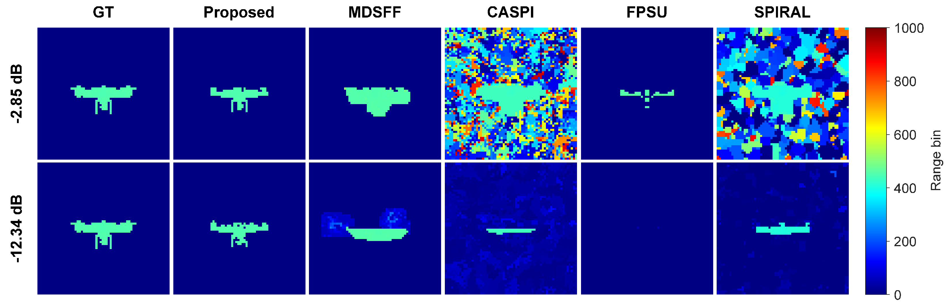
The SBR simulations assess target-structure preservation as the background-event fraction increases. Figure 6 compares the ground truth with range maps from five methods at −2.85 and −12.34 dB.

At −2.85 dB, background-corrected multi-scale local statistics support trajectory estimation. Accumulation along the estimated range-time trajectory recovers the UAV body, arms, and lower structure, while confining background responses to a relatively small region. At −12.34 dB, the main target structure remains at the ground-truth position. MDSFF yields an enlarged target region. CASPI and SPIRAL retain broader background ranges, whereas FSPU retains only a few pixels. These observations require joint consideration of target completeness, range structure, and background false positives.

Table 3. Quantitative results for the low-SBR simulation at −12.34 dB.

Method	SSIM ↑	RMSE (Range Bins) ↓	PSNR ↑	IoU ↑	FPR (%) ↓
Proposed	0.61	223.22	6.36	0.74	0.10
MDSFF	0.01	312.19	3.44	0.26	8.07
CASPI	0.11	367.14	2.03	0.04	100.00
FSPU	0.00	452.75	0.21	0.01	0.00
SPIRAL	0.28	322.14	3.17	0.04	100.00

Note: ↑ indicates that a higher value is better, whereas ↓ indicates that a lower value is better.

reports the corresponding five-metric comparison for the −12.34 dB case.

At −12.34 dB, the method achieves SSIM, RMSE (range bins), PSNR, IoU, and FPR values of 0.61, 223.22, 6.36 dB, 0.74, and 0.10%, respectively. MDSFF yields an IoU of 0.26 and an FPR of 8.07%, consistent with its larger predicted target region. FSPU has an FPR of 0% but an IoU of only 0.01, showing the limited value of a false-positive metric for a nearly empty output. Under the present evaluation rule, CASPI and SPIRAL both reach an FPR of 100%. Range structure, target-region overlap, and background control should therefore be assessed together.

5.2. Simulation Results at Different Range-Bin Drift Rates

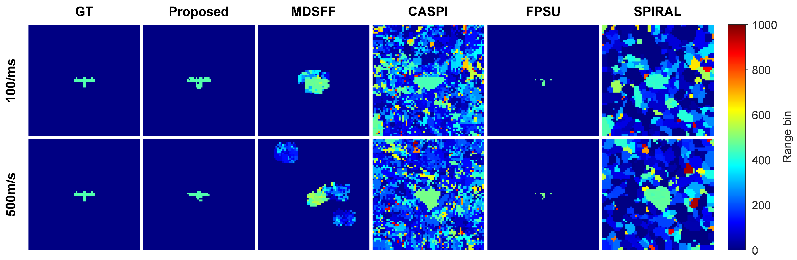
To assess range migration caused by line-of-sight motion, simulations were conducted at 100 and 500 m/s under the same background-noise influence. Figure 7 compares the ground truth, the proposed method, and four external methods within a common display range.

At 100 and 500 m/s, the method recovers a connected main target structure at the correct position with few external responses. Background-corrected multi-scale local statistics support trajectory estimation, and accumulation along the estimated migration path reduces fixed-bin event dispersion. MDSFF shows contour expansion at 100 m/s and several isolated response clusters at 500 m/s. CASPI and SPIRAL retain broad background responses, whereas FSPU yields a nearly empty output. Across the tested range migration conditions, the target structure remains preserved. The comparison does not establish a monotonic dependence on velocity.

Table 4. Quantitative results of the proposed method at different line-of-sight velocities.

Line-of-Sight Velocity	SSIM ↑	RMSE (Range Bins) ↓	PSNR ↑	IoU ↑	FPR (%) ↓
100 m/s	0.57	134.19	10.61	0.73	0.44
500 m/s	0.78	173.80	8.36	0.60	0.12

Note: ↑ indicates that a higher value is better, whereas ↓ indicates that a lower value is better.

summarizes the proposed method’s metrics at the two tested line-of-sight velocities.

At 100 and 500 m/s, the method achieves IoU values of 0.73 and 0.60 and FPR values of 0.44% and 0.12%, respectively. These point estimates suggest relatively complete target-region recovery at both velocities but do not imply a monotonic velocity dependence. Monte Carlo event realization, target scale, and valid-photon count can affect each result. Establishing a velocity response requires independent repetitions under matched statistical conditions, with both means and dispersion reported.

5.3. Multimetric Comparison

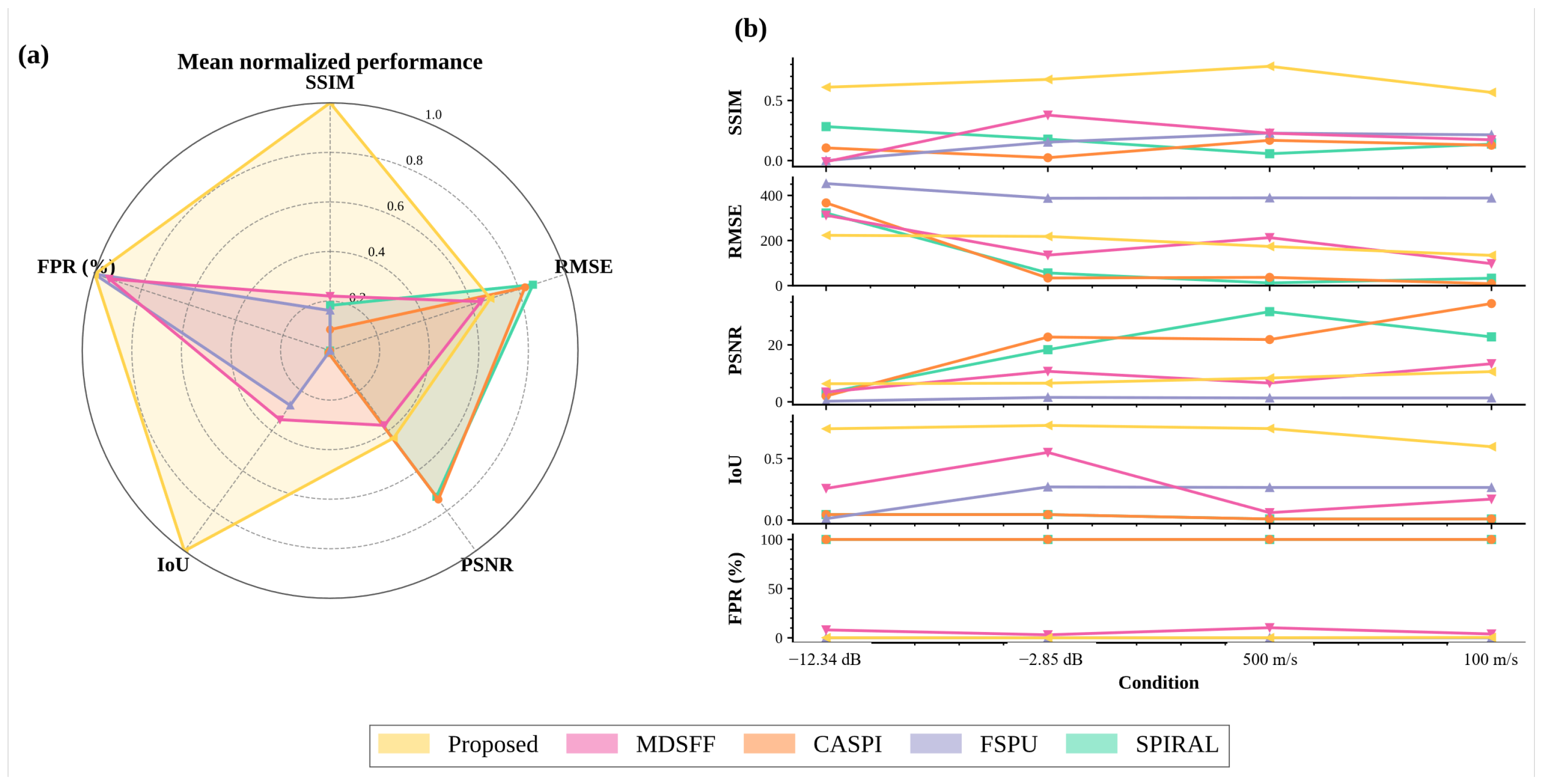
Figure 8 compares five metrics across two SBRs and two velocities. Normalization is performed separately within each of the four simulation conditions and for each metric, using the five compared methods to define $x_{min}$ and $x_{max}$. For SSIM, PSNR, and IoU, the normalized score is $(x-x_{min})/(x_{max}-x_{min})$. For RMSE (range bins) and FPR, the direction is reversed, giving $(x_{max}-x)/(x_{max}-x_{min})$, so that a larger score is always better. For each method, the five normalized metric scores are averaged within each condition, and the four condition-level scores are then averaged to obtain the reported mean five-metric score. Equivalently, each radar-chart spoke is the mean normalized value of one metric across the four conditions. The line plot retains the original units and exposes trade-offs among metrics.

In Figure 8a, the method attains a mean normalized five-metric score of 0.82 across structural preservation, target-region overlap, and background control. The corresponding scores for MDSFF, SPIRAL, CASPI, and FSPU are 0.50, 0.36, 0.33, and 0.29. Figure 8b reveals that stronger performance in one range metric can coincide with lower IoU or higher FPR. The normalized score summarizes metric trade-offs but does not replace individual results or statistical significance tests.

5.4. Low-SBR Reconstruction of Evaluation Cases Derived from Measured Sequences

Table 5. Five-metric results for five methods across 19 experimentally generated low-SBR evaluation cases derived from measured GM-APD LiDAR sequences (mean ± standard deviation). The standard deviation combines variation among degradation conditions and variation from random repetitions; it does not represent repeated measurements under one identical condition.

Method	SSIM ↑	RMSE (Range Bins) ↓	PSNR ↑ (dB)	IoU ↑	FPR ↓ (%)
Proposed	$0.541\pm 0.165$	$332.93\pm 79.60$	$8.60\pm 2.49$	$0.702\pm 0.061$	$0.33\pm 0.08$
MDSFF	$0.003\pm 0.002$	$621.43\pm 1.38$	$2.88\pm 0.02$	$0.017\pm 0.000$	$100.00\pm 0.00$
CASPI	$0.139\pm 0.291$	$582.61\pm 159.27$	$3.88\pm 3.11$	$0.017\pm 0.000$	$100.00\pm 0.00$
FSPU	$0.313\pm 0.356$	$389.63\pm 150.98$	$7.59\pm 3.51$	$0.033\pm 0.007$	$53.86\pm 14.24$
SPIRAL	$0.121\pm 0.244$	$604.25\pm 165.68$	$3.57\pm 3.13$	$0.017\pm 0.000$	$100.00\pm 0.00$

Note: ↑ indicates that a higher value is better, whereas ↓ indicates that a lower value is better.

summarizes five methods across 19 experimentally generated low-SBR evaluation cases derived from measured GM-APD LiDAR sequences. Temporal resampling, target-event retention, and background-event injection defined the evaluated conditions. SSIM, RMSE (range bins), and PSNR quantified range structure and error within the reference region. IoU and FPR quantified full-field target-region overlap and background false positives. Reported means and standard deviations include variation across degradation conditions and random repetitions. These cases were controlled transformations of measured sequences rather than independent field acquisitions.

Across the 19 evaluation cases, the method obtained mean SSIM, RMSE (range bins), PSNR, IoU, and FPR values of 0.541, 332.93, 8.60 dB, 0.702, and 0.33%, respectively. FSPU, for comparison, obtained an RMSE of 389.63 range bins, an IoU of 0.033, and an FPR of 53.86%. Under the present protocol, background-corrected multi-scale local statistics and trajectory-guided photon accumulation recovered a concentrated target region and pixel-wise range information. This behavior persisted when practical detection noise and motion-induced range migration coexisted.

MDSFF, CASPI, and SPIRAL return finite ranges across almost the full field, while FSPU produces a large, partly dense region. Differences in output task therefore affect their IoU and FPR values. The reported values apply only to the target range-recovery task evaluated here and do not characterize general full-field range recovery.

For G01, SSIM, RMSE (range bins), PSNR, IoU, and FPR are 0.894, 136.25, 16.06 dB, 0.744, and 0.273%, respectively. G07 uses 10× temporal resampling and the lowest event-retention ratio, giving corresponding values of 0.366, 410.60, 6.51 dB, 0.659, and 0.381%. Range-structure metrics change more from G01 to G07 than target-region metrics, suggesting that internal range detail depends more strongly on valid-event count. Because temporal resampling and event sparsity vary together, the comparison does not isolate a single-factor velocity effect.

Table 6. Results for low-SBR cases derived from measured sequences minus the mean results for four simulation conditions. Positive ΔRMSE (range bins) and ΔFPR denote increased error or false positives; negative values for the other metrics denote reduced performance.

Method	$\mathbf{\Delta }$SSIM	$\mathbf{\Delta }$RMSE (Range Bins)	$\mathbf{\Delta }$PSNR (dB)	$\mathbf{\Delta }$IoU	$\mathbf{\Delta }$FPR (Percentage Points)
Proposed	−0.118	+145.58	+0.63	−0.010	+0.16
MDSFF	−0.189	+431.94	−5.65	−0.242	+93.66
CASPI	+0.033	+471.05	−16.40	−0.009	0.00
FSPU	+0.164	−14.88	+6.47	−0.170	+53.86
SPIRAL	−0.043	+498.42	−15.41	−0.009	0.00

compares the evaluation cases derived from measured sequences with the mean of the four simulation conditions. For the method, IoU decreased by 0.010, FPR increased by 0.16 percentage points, and SSIM decreased by 0.118. The small IoU and FPR changes were consistent with similar target-region recovery and background control across the two data types. The SSIM decrease reflected detector nonuniformity, event sparsity, and interframe range migration within the reconstructed range structure. These values describe only the difference between data domains.

RMSE (range bins) increases by 145.58, although the simulated and measured data cover different range spans. The absolute difference therefore does not directly quantify cross-domain performance. Normalization by the respective reference ranges gives dimensionless normalized RMSE values of 0.407 and 0.384, a difference of −0.023. Cross-domain comparison should consider normalized range error together with IoU and FPR.

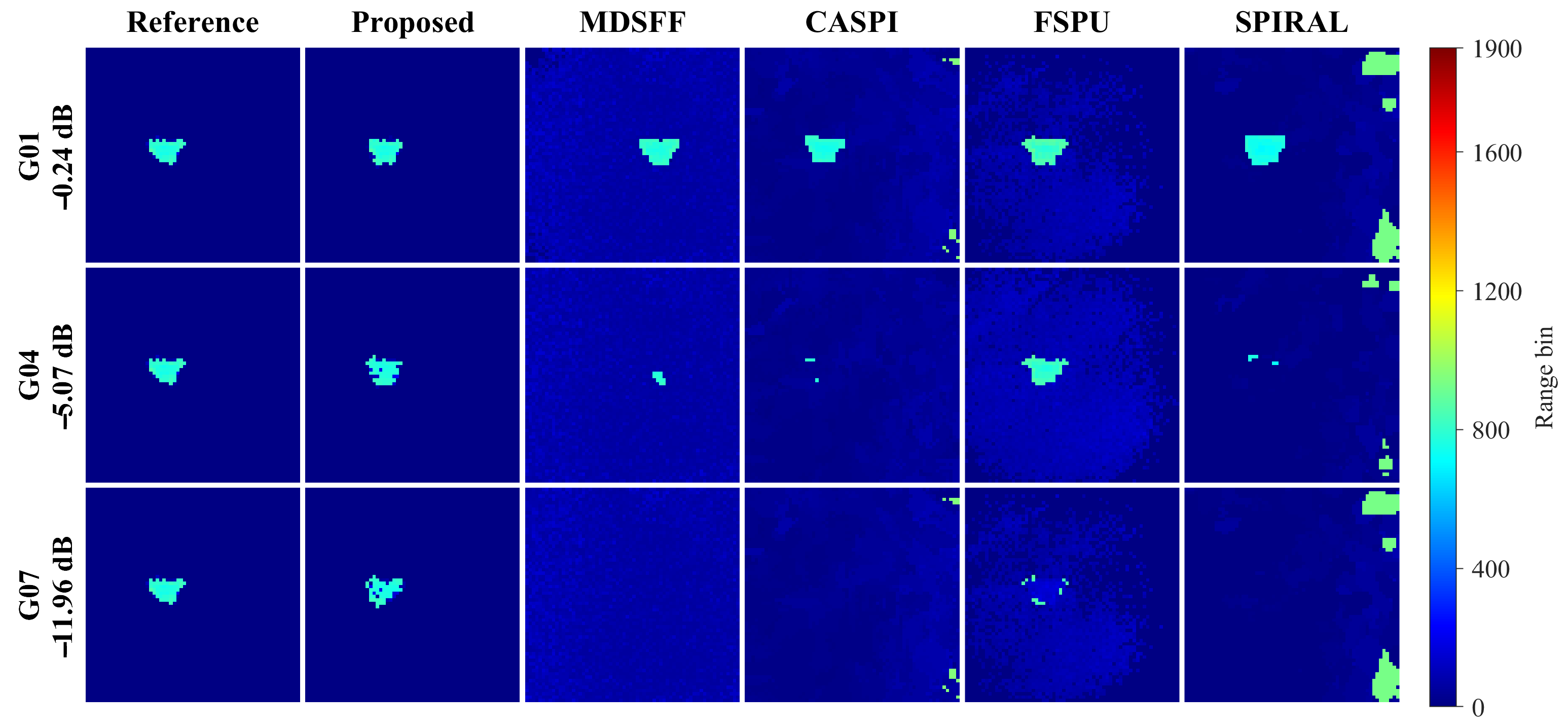
Figure 9 spans the original dynamic observation (G01) and the stronger combined degradations in G04 and G07. Increasing temporal resampling and decreasing target-event retention produce greater range-bin migration. Fixed-bin accumulation then becomes more susceptible to range-peak broadening and local fragmentation. The method uses multi-scale local statistics to suppress random background responses and accumulates interframe events along the estimated migration path. All three conditions yield a single concentrated target region whose position agrees with the manual reference. The external methods retain the main target structure under some conditions but produce broader background range responses.

Across 19 evaluation cases, the method retained an average of 72 finite-valued range pixels. MDSFF, CASPI, FSPU, and SPIRAL retained approximately 4096, 4096, 2238, and 4096 pixels, respectively. Under the present evaluation, broad finite-range outputs counted as background false positives. Figure 9 and Table 5 therefore compare target completeness, range consistency, and background control only for this weak-target range-recovery task.

6. Discussion

The method addresses two coupled limitations of photon-efficient active remote sensing: low-SBR detection and motion-induced range migration. The range-dependent background probability estimates the nontarget event level in each range bin. Background-corrected multi-scale statistics reduce contamination without discarding spatial localization or weak-event continuity. The estimated range-time path identifies the frame-dependent echo bin and guides the accumulation of returns that would otherwise remain dispersed. Cross-scale response fusion then constrains the weak-target range interval and spatial region before pixel-wise range recovery. This sequence may explain why the method retained spatial structure while suppressing background responses under the tested conditions. Previous analyses of high-flux operation and depth-imaging limits likewise show that photon-observation rules and available event counts jointly constrain ranging accuracy [12,13].

The proposed method provides a potential solution for photon-limited reconstruction when weak returns are distributed across range-time dimensions. The combination of background correction, migration-aware accumulation, and spatial-range fusion could support airborne inspection, long-range observation, and weak-target observation. These are prospective engineering uses rather than applications validated by the present experiments. The current evidence comprises controlled simulations and 19 low-SBR evaluation cases generated from measured GM-APD LiDAR sequences. These cases are not independent field acquisitions. Field deployment would additionally require evaluation of platform motion, atmospheric variability, calibration drift, and scene complexity.

The external methods emphasize complementary reconstruction principles. MDSFF uses multidomain feature fusion, CASPI uses collaborative photon processing [27,28], FSPU uses first-signal-photon selection [29], and SPIRAL uses sparse Poisson inversion [30]. The present method instead uses deterministic interframe range migration as an accumulation constraint. Multi-scale local statistics separate weak-target events from range-dependent background. Bounded trajectory parameter optimization using PSO is confined to the three migration parameters. Alternative bounded search strategies may affect runtime and convergence, but they do not alter the range-time migration model, trajectory-guided accumulation, or subsequent region and range recovery.

Three limitations define the scope of the results. First, the tested SBR and line-of-sight velocity conditions are too limited to establish complete response curves or statistically isolate either factor. Second, the measured-sequence reference combines the original dynamic sequence with a manually annotated target region and is not independent synchronized ranging ground truth. Third, temporal resampling increases line-of-sight range migration but does not represent complete six-degree-of-freedom motion. The experimentally generated low-SBR cases cannot replace original low-SBR field acquisitions. Future evaluation should include synchronized ranging truth, independently varied SBR and velocity, transverse pixel migration, attitude changes, atmospheric perturbations, and additional targets and acquisition distances.

7. Conclusions

This work presents a photon-efficient active LiDAR remote sensing method for photon-limited reconstruction with a 1064 nm InGaAs/InP $64\times 64$ GM-APD array. Its central contribution is to use deterministic range-time migration as a constraint for aligning and accumulating weak interframe events. Range-dependent background correction and multi-scale local photon statistics suppress nonuniform detections while preserving weak-event stability and spatial localization. A band-shaped trajectory model and bounded trajectory parameter optimization using PSO estimate the range-bin drift rate, initial range position, and trajectory-band half-width. Cross-scale fusion then recovers the weak-target range interval, reconstruction mask, pixel-wise range values, and confidence map.

At −12.34 dB in simulation, the method achieved SSIM, RMSE (range bins), PSNR, IoU, and FPR values of 0.61, 223.22, 6.36 dB, 0.74, and 0.10%, respectively. Across 19 experimentally generated low-SBR evaluation cases derived from measured GM-APD LiDAR sequences, the corresponding mean values were $0.541\pm 0.165$, $332.93\pm 79.60$, $8.60\pm 2.49$ dB, $0.702\pm 0.061$, and $0.33\pm 0.08$%. Under the tested conditions, these results indicate the potential value of migration-aware photon accumulation for active remote sensing when limited returns are dispersed by scene dynamics. Broader deployment requires independent ranging truth and more diverse platform, atmosphere, distance, and motion conditions.

References

1. Piron, F.; Morrison, D.; Yuce, M.R.; Redouté, J.M. A Review of Single-Photon Avalanche Diode Time-of-Flight Imaging Sensor Arrays. IEEE Sens. J. 2021, 21, 12654–12666. [Google Scholar] [CrossRef] [Scilit]
2. Tan, C.; Kong, W.; Huang, G.; Jia, S.; Liu, Q.; Han, Q.; Hou, J.; Xue, R.; Yu, S.; Shu, R. Development of a Near-Infrared Single-Photon 3D Imaging LiDAR Based on 64 × 64 InGaAs/InP Array Detector and Risley-Prism Scanner. Opt. Express 2024, 32, 7426–7447. [Google Scholar] [CrossRef] [Scilit] [PubMed]
3. Chi, K.; Liu, X.; Kong, W.; Xue, R.; Huang, G. Few-Photon Pixel-Level Target Detection Imaging Based on 64 × 64 Array GM-APD Lidar System. Infrared Phys. Technol. 2025, 146, 105722. [Google Scholar] [CrossRef] [Scilit]
4. Zhang, X.; Sun, J.; Li, S.; Zhang, Y.; Liu, D.; Zhang, H. Research on the Detection Probability Curve Characteristics of Long-Range Target Based on SPAD Array Lidar. Infrared Phys. Technol. 2022, 126, 104325. [Google Scholar] [CrossRef] [Scilit]
5. Degnan, J.J. Scanning, Multibeam, Single Photon Lidars for Rapid, Large Scale, High Resolution, Topographic and Bathymetric Mapping. Remote Sens. 2016, 8, 958. [Google Scholar] [CrossRef] [Scilit]
6. Popescu, S.C.; Zhou, T.; Nelson, R.; Neuenschwander, A.; Sheridan, R.; Narine, L.; Walsh, K.M. Photon Counting LiDAR: An Adaptive Ground and Canopy Height Retrieval Algorithm for ICESat-2 Data. Remote Sens. Environ. 2018, 208, 154–170. [Google Scholar] [CrossRef] [Scilit]
7. Neumann, T.A.; Martino, A.J.; Markus, T.; Bae, S.; Bock, M.R.; Brenner, A.C.; Brunt, K.M.; Cavanaugh, J.; Fernandes, S.T.; Hancock, D.W.; et al. The Ice, Cloud, and Land Elevation Satellite-2 Mission: A Global Geolocated Photon Product Derived from the Advanced Topographic Laser Altimeter System. Remote Sens. Environ. 2019, 233, 111325. [Google Scholar] [CrossRef] [Scilit] [PubMed]
8. Ma, Y.; Zhang, W.; Sun, J.; Li, G.; Wang, X.H.; Li, S.; Xu, N. Photon-Counting Lidar: An Adaptive Signal Detection Method for Different Land Cover Types in Coastal Areas. Remote Sens. 2019, 11, 471. [Google Scholar] [CrossRef] [Scilit]
9. Incoronato, A.; Locatelli, M.; Zappa, F. Statistical Modelling of SPADs for Time-of-Flight LiDAR. Sensors 2021, 21, 4481. [Google Scholar] [CrossRef] [Scilit] [PubMed]
10. Coates, P.B. The Correction for Photon `Pile-Up’ in the Measurement of Radiative Lifetimes. J. Phys. E Sci. Instrum. 1968, 1, 878–879. [Google Scholar] [CrossRef] [Scilit]
11. Chang, J.; Chen, K.; Li, J.; Yan, C.; Wang, Y.; Zhong, K.; Xu, D.; Yao, J. GM-APD Lidar Target Scattering Feature Calculation and Analysis Based on Radiometric Calibration Model. Infrared Phys. Technol. 2025, 150, 105930. [Google Scholar] [CrossRef] [Scilit]
12. Rapp, J.; Ma, Y.; Dawson, R.M.A.; Goyal, V.K. High-Flux Single-Photon Lidar. Optica 2021, 8, 30–39. [Google Scholar] [CrossRef] [Scilit]
13. Scholes, S.; Mora-Martín, G.; Zhu, F.; Gyongy, I.; Soan, P.; Leach, J. Fundamental Limits to Depth Imaging with Single-Photon Detector Array Sensors. Sci. Rep. 2023, 13, 176. [Google Scholar] [CrossRef] [Scilit] [PubMed]
14. Tobin, R.; Halimi, A.; McCarthy, A.; Soan, P.J.; Buller, G.S. Robust Real-Time 3D Imaging of Moving Scenes through Atmospheric Obscurant Using Single-Photon LiDAR. Sci. Rep. 2021, 11, 11236. [Google Scholar] [CrossRef] [Scilit] [PubMed]
15. Liu, D.; Sun, J.; Lu, W.; Li, S.; Zhou, X. 3D Reconstruction of the Dynamic Scene with High-Speed Targets for GM-APD LiDAR. Opt. Laser Technol. 2023, 161, 109114. [Google Scholar] [CrossRef] [Scilit]
16. Zhang, X.; Li, S.; Sun, J.; Ma, L.; Zhou, X.; Yang, X.; He, R. Dynamic Target Feature Selection in Pixel Change Space for Array GM-APD Lidar. Infrared Phys. Technol. 2024, 140, 105396. [Google Scholar] [CrossRef] [Scilit]
17. Wu, C.; Xing, W.; Feng, Z.; Xia, L. Moving Target Tracking in Marine Aerosol Environment with Single Photon Lidar System. Opt. Lasers Eng. 2020, 127, 105967. [Google Scholar] [CrossRef] [Scilit]
18. Guo, D.; Qu, Y.; Zhou, X.; Sun, J.; Yin, S.; Lu, J.; Liu, F. Research on Automatic Tracking and Size Estimation Algorithm of “Low, Slow and Small” Targets Based on Gm-APD Single-Photon LIDAR. Drones 2025, 9, 85. [Google Scholar] [CrossRef] [Scilit]
19. Kirmani, A.; Venkatraman, D.; Shin, D.; Colaço, A.; Wong, F.N.C.; Shapiro, J.H.; Goyal, V.K. First-Photon Imaging. Science 2014, 343, 58–61. [Google Scholar] [CrossRef] [Scilit] [PubMed]
20. Altmann, Y.; Ren, X.; McCarthy, A.; Buller, G.S.; McLaughlin, S. Lidar Waveform-Based Analysis of Depth Images Constructed Using Sparse Single-Photon Data. IEEE Trans. Image Process. 2016, 25, 1935–1946. [Google Scholar] [CrossRef] [Scilit] [PubMed]
21. Altmann, Y.; Ren, X.; McCarthy, A.; Buller, G.S.; McLaughlin, S. Robust Bayesian Target Detection Algorithm for Depth Imaging from Sparse Single-Photon Data. IEEE Trans. Comput. Imaging 2016, 2, 456–467. [Google Scholar] [CrossRef] [Scilit]
22. Rapp, J.; Goyal, V.K. A Few Photons among Many: Unmixing Signal and Noise for Photon-Efficient Active Imaging. IEEE Trans. Comput. Imaging 2017, 3, 445–459. [Google Scholar] [CrossRef] [Scilit]
23. Tachella, J.; Altmann, Y.; Ren, X.; McCarthy, A.; Buller, G.S.; McLaughlin, S.; Tourneret, J.Y. Bayesian 3D Reconstruction of Complex Scenes from Single-Photon Lidar Data. SIAM J. Imaging Sci. 2019, 12, 521–550. [Google Scholar] [CrossRef] [Scilit]
24. Tachella, J.; Altmann, Y.; Mellado, N.; McCarthy, A.; Tobin, R.; Buller, G.S.; Tourneret, J.Y.; McLaughlin, S. Real-Time 3D Reconstruction from Single-Photon Lidar Data Using Plug-and-Play Point Cloud Denoisers. Nat. Commun. 2019, 10, 4984. [Google Scholar] [CrossRef] [Scilit] [PubMed]
25. Chen, S.; Halimi, A.; Ren, X.; McCarthy, A.; Su, X.; McLaughlin, S.; Buller, G.S. Learning Non-Local Spatial Correlations to Restore Sparse 3D Single-Photon Data. IEEE Trans. Image Process. 2020, 29, 3119–3131. [Google Scholar] [CrossRef] [PubMed]
26. Peng, J.; Xiong, Z.; Tan, H.; Huang, X.; Li, Z.P.; Xu, F. Boosting Photon-Efficient Image Reconstruction with a Unified Deep Neural Network. IEEE Trans. Pattern Anal. Mach. Intell. 2023, 45, 4180–4197. [Google Scholar] [CrossRef] [Scilit] [PubMed]
27. Ma, L.; Sun, J.; Yang, X.; Lu, J.; Lu, W.; Zhou, X.; Ni, H. Reconstruction Method of 128 × 256 Array Single Photon Lidar Based on Multi-Domain Stability Feature Fusion. Opt. Laser Technol. 2025, 181, 111970. [Google Scholar] [CrossRef] [Scilit]
28. Lee, J.; Ingle, A.; Chacko, J.V.; Eliceiri, K.W.; Gupta, M. CASPI: Collaborative Photon Processing for Active Single-Photon Imaging. Nat. Commun. 2023, 14, 3158. [Google Scholar] [CrossRef] [Scilit] [PubMed]
29. Hua, K.; Liu, B.; Chen, Z.; Fang, L.; Wang, H. Efficient and Noise Robust Photon-Counting Imaging with First Signal Photon Unit Method. Photonics 2021, 8, 229. [Google Scholar] [CrossRef] [Scilit]
30. Harmany, Z.T.; Marcia, R.F.; Willett, R.M. This Is SPIRAL-TAP: Sparse Poisson Intensity Reconstruction Algorithms–Theory and Practice. IEEE Trans. Image Process. 2012, 21, 1084–1096. [Google Scholar] [CrossRef] [Scilit] [PubMed]
31. Kennedy, J.; Eberhart, R. Particle Swarm Optimization. In Proceedings of the ICNN’95—International Conference on Neural Networks, Perth, WA, Australia, 27 November–1 December 1995; Volume 4, pp. 1942–1948. [Google Scholar] [CrossRef] [Scilit]
32. Gyongy, I.; Dutton, N.A.W.; Henderson, R.K. Direct Time-of-Flight Single-Photon Imaging. IEEE Trans. Electron Devices 2022, 69, 2794–2805. [Google Scholar] [CrossRef] [Scilit]
33. Koerner, L.J. Models of Direct Time-of-Flight Sensor Precision That Enable Optimal Design and Dynamic Configuration. IEEE Trans. Instrum. Meas. 2021, 70, 8502609. [Google Scholar] [CrossRef] [Scilit]
34. Wang, Z.; Bovik, A.C.; Sheikh, H.R.; Simoncelli, E.P. Image Quality Assessment: From Error Visibility to Structural Similarity. IEEE Trans. Image Process. 2004, 13, 600–612. [Google Scholar] [CrossRef] [Scilit] [PubMed]
Figure 1. Range migration under line-of-sight motion. (a) Range-stable target. (b) Target undergoing line-of-sight motion. (c) Peak broadening caused by fixed-bin accumulation. (d) Compact response obtained by accumulation along the migration path. In panels (a) and (b), the red and blue arrows denote the outgoing laser pulse and returning photons, respectively, and the red arrow above the target in panel (b) denotes line-of-sight velocity. In panel (c), the blue, orange, and green curves are representative frame-wise range responses, whereas the red curve is their direct fixed-bin accumulation. In panel (d), the green curve is the trajectory-constrained reconstructed response and the blue dashed vertical line marks its estimated peak range bin.
Remotesensing 18 03007 g001
Figure 2. Workflow of range-time trajectory-guided photon accumulation for dynamic LiDAR remote sensing reconstruction.
Remotesensing 18 03007 g002
Figure 3. Background-corrected multi-scale local range-time statistics. (a) Local windows on the 64 × 64 array. (bd) Background-corrected range-time matrices obtained using 4 × 4, 8 × 8, and 16 × 16 spatial windows, respectively. In panels (bd), the horizontal axis is the frame index m, the vertical axis is the range-bin index , and the color scale from 0 to 1 shows the normalized background-corrected response after logarithmic compression and smoothing. Warmer colors indicate stronger responses above the estimated background level. The continuous high-response band represents target range migration across frames. The red, orange, and blue boxes and arrows link the 4 × 4, 8 × 8, and 16 × 16 windows in panel (a) to panels (b), (c), and (d), respectively.
Remotesensing 18 03007 g003
Figure 4. Trajectory parameter optimization and photon accumulation. (a) Candidate trajectory band with flanking background bands. (b) Bounded optimization in the θ = [ α , β , δ ] parameter space. (c) Components of the regional trajectory score. In panel (a), the solid white line is the trajectory center, the yellow dashed lines are the candidate-band boundaries, the white dotted lines delimit the flanking background bands, and the red points are particle candidates. In panel (b), the blue points are particles, the gray arrows indicate their updates, and the orange point is the best candidate. Panel (c) shows the positive evidence and penalty components of the regional score.
Remotesensing 18 03007 g004
Figure 5. Cross-scale response fusion and target localization. (a) Multi-scale local evidence. (b) Regional trajectory candidates. (c) Parameter-space clustering. (d) Joint range and region recovery. In panel (a), the red, orange, and blue boxes denote the 4 × 4, 8 × 8, and 16 × 16 windows, respectively. In panel (b), the colored lines denote regional trajectory candidates and C i denotes candidate confidence. In panel (c), the colored points denote trajectory-parameter clusters, and the red ellipse marks the selected highest-confidence cluster G * ; the asterisk identifies this selected cluster. In panel (d), the green outlines show the overlapping candidate regions, whereas the blue line and shaded band denote the fused trajectory and its support.
Remotesensing 18 03007 g005
Figure 6. UAV target range reconstruction at −2.85 and −12.34 dB. Columns show the ground truth, proposed method, MDSFF, CASPI, FSPU, and SPIRAL results.
Remotesensing 18 03007 g006
Figure 7. UAV target range reconstruction at line-of-sight velocities of 100 and 500 m/s. Columns show the ground truth, proposed method, MDSFF, CASPI, FSPU, and SPIRAL results.
Remotesensing 18 03007 g007
Figure 8. Multimetric performance under four simulation conditions. (a) Direction-aligned normalized mean scores. For each condition and metric, min–max normalization is performed across the five methods before averaging across the four conditions. (b) Original SSIM, RMSE (range bins), PSNR, IoU, and FPR values.Colors and marker shapes identify the five methods as shown in the legend; lines connect results from the same method across conditions, and the marker shapes do not encode additional variables.
Remotesensing 18 03007 g008
Figure 9. Reconstruction results for low-SBR evaluation cases derived from measured GM-APD LiDAR sequences. Rows 1–3 correspond to G01, G04, and G07 with increasing range migration and decreasing SBR. Columns show the reference, proposed method, MDSFF, CASPI, FSPU, and SPIRAL results.
Remotesensing 18 03007 g009