Surface Thermal State, Antecedent Hydroclimate, and Post-Fire Vegetation–Water Response in the Zambezi River Basin: A Multi-Source Environmental Time-Series Analysis

Highlights

What are the main findings?

• Warmer daytime land surface temperature (LST) and lower near-surface soil moisture are robustly associated with larger same-month burned-area anomalies, while antecedent precipitation and soil-moisture histories carry the strongest 1–9 month signal.
• Burned-area history is followed by delayed basin-wide declines in normalized difference vegetation index (NDVI) and evapotranspiration (ET), but effect magnitude and statistical certainty vary among Level-4 sub-basins.

What are the implications of the main findings?

• Basin-scale fire inference should separate short-horizon surface state, antecedent hydroclimate, and post-fire response rather than assign one mechanistic role to each correlated environmental variable.
• Temporal cross-validation, multiplicity control, product sensitivity, and sub-basin robustness materially constrain claims that would otherwise appear stronger in a single basin-average analysis.

Abstract

Wildfire in African savannas reflects coupled surface thermal, hydroclimatic, vegetation, and disturbance processes, but basin-scale time-series analyses can overstate mechanisms when temporal dependence and spatial heterogeneity are ignored. We assembled a monthly 2003–2024 multi-source environmental dataset for the Zambezi River Basin ($n=263$) and nine Level-4 HydroBASINS units, using quality-controlled MODIS burned area, normalized difference vegetation index (NDVI), daytime land surface temperature (LST), and evapotranspiration (ET), together with CHIRPS precipitation and GLDAS-2.1 Noah 0–10 cm soil moisture. Primary inference used heteroskedasticity- and autocorrelation-consistent regressions, expanding-window Random Forest validation, false-discovery-rate-controlled distributed-lag tests, and sub-basin robustness; vector autoregression was retained as a secondary diagnostic. Current-month burned-area anomalies were positively associated with LST ($\beta =0.340$, $p=0.0015$) and negatively associated with near-surface soil moisture ($\beta =-0.326$, $p=0.0005$). Over 1–9 months, precipitation and soil-moisture histories were jointly supported after multiplicity correction, whereas basin-wide NDVI, ET, and LST histories were not. Burned-area history was followed by cumulative 0–6 month declines in NDVI ($\beta =-0.280$, 95% CI $[-0.452,-0.107]$) and ET ($\beta =-0.214$, 95% CI $[-0.419,-0.008]$). Directions were broadly consistent across sub-basins, although magnitudes varied. The evidence supports time-scale-specific conditional associations without structural-causal claims.

1. Introduction

Wildfire is a fundamental ecological process that regulates vegetation structure, biogeochemical cycling, and land–atmosphere exchange across savannas and drylands [1,2]. Africa contributes a dominant share of global burned area, and southern African fire regimes are shaped jointly by climate, vegetation productivity, fuel continuity, ignition, and human land management [3,4,5,6]. This combination makes African savannas especially important for testing how hydroclimatic variability and vegetation state are related to fire across multiple time scales.

A persistent difficulty is that the physical variables relevant to fire are strongly coupled. Wet conditions can suppress burning in the near term by increasing surface and fuel moisture, while the same wet period can promote later vegetation production and fuel continuity [7,8,9]. Surface temperature likewise responds to radiation, vegetation cover, soil moisture, turbulent exchange, and atmospheric demand; land surface temperature (LST) therefore cannot be treated as a direct substitute for air temperature or vapor pressure deficit [10,11]. Normalized difference vegetation index (NDVI) measures optical greenness rather than fuel mass or live-fuel water content, and evapotranspiration (ET) represents a coupled land–atmosphere water flux rather than a direct measure of water availability. These distinctions are essential when statistical lag relationships are interpreted physically.

The same caution applies after fire. Disturbance can alter canopy cover, surface energy partitioning, vegetation greenness, transpiration, and plant–soil water relations, but the sign and duration of observed responses depend on biome, fire severity, phenology, and the remote-sensing quantity being measured [12,13,14,15,16]. A return of NDVI toward its climatological state, for example, does not necessarily imply recovery of biomass, woody structure, or vegetation water content [15,17]. Consequently, terms such as “hydrologic mediation” and “post-fire memory” require stronger process identification than a predictive time-series model alone can provide.

Methodological choices can further amplify apparent evidence. Random Forests capture nonlinearities and interactions but can redistribute importance among correlated predictors and can overstate generalization if temporally autocorrelated observations are randomly split [18,19]. High-order vector autoregressions (VARs) become parameter intensive in short monthly records, while individual lag coefficients and repeated Granger tests raise multiplicity concerns [20,21,22]. Impulse-response functions are also sensitive to contemporaneous identification, and none of these reduced-form tools establish structural causality in the presence of omitted fire-weather, ignition, land-use, and management variables.

The Zambezi River Basin provides a useful regional setting for a more constrained analysis. The basin spans approximately 1.38 million km² across eight southern African countries and crosses pronounced hydroclimatic gradients from wetter northern headwaters to semi-arid southern and eastern landscapes. Rainfall is strongly seasonal and linked to the migration of the Intertropical Convergence Zone, while fire activity commonly intensifies during the dry season as vegetation cures and surface moisture declines [23,24]. 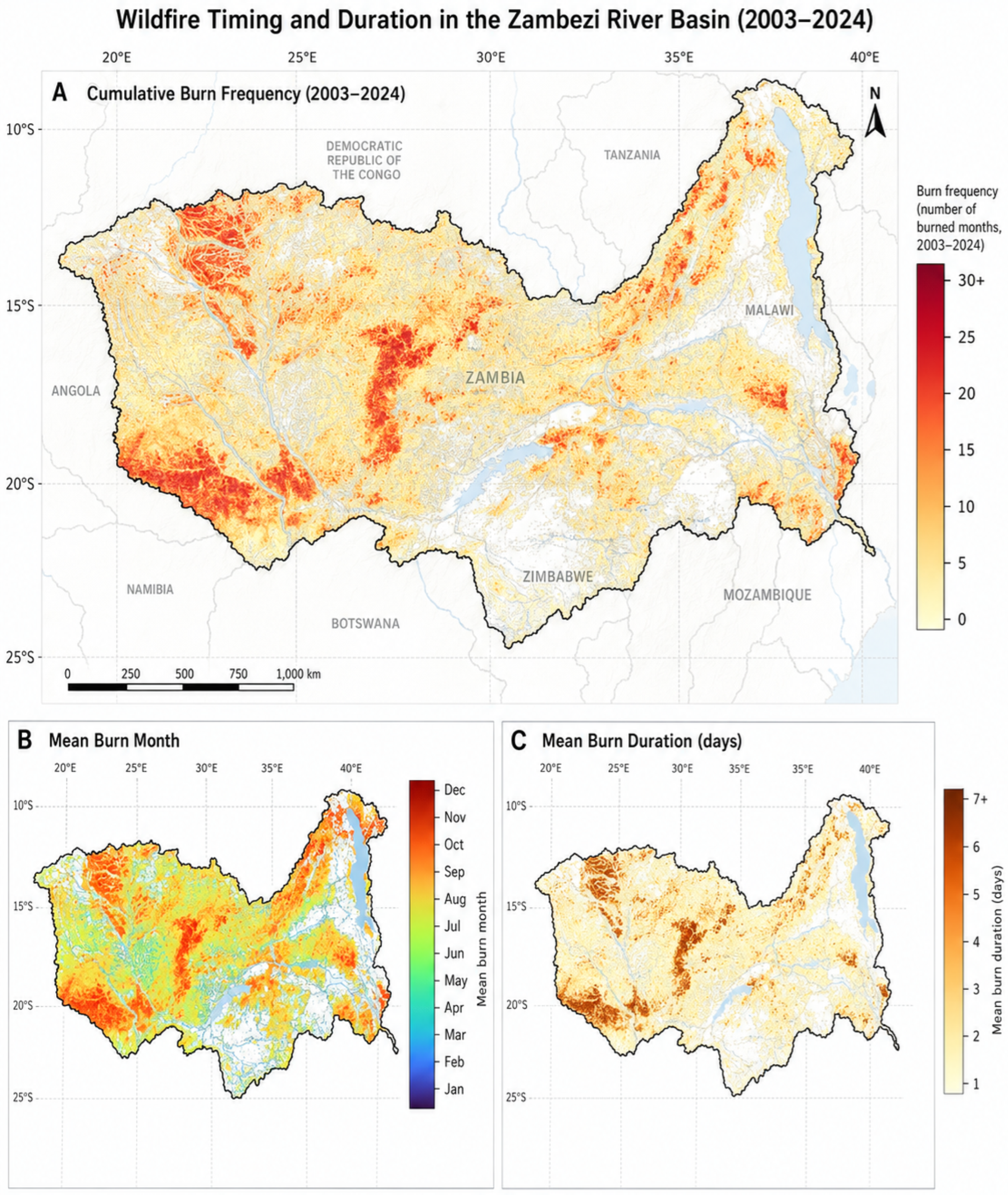Figure 1 illustrates the basin’s spatially heterogeneous fire context.

The analysis is organized around three explicitly testable hypotheses, each tied to variables, directions, lag windows, and evidentiary criteria (

Table 1. Hypotheses, variables, lag windows, and criteria used in the analysis.

Hypothesis	Target Relationship	Expected Evidence	Decision Criteria
H1	Current burned-area anomaly versus daytime LST and near-surface soil moisture; current and 1-month controls included.	${\beta }_{\mathrm{LST},t}>0$; ${\beta }_{\mathrm{SM},t}<0$.	Expected signs with HAC uncertainty; stability to precipitation/soil-moisture product substitutions, cropland-NDVI substitution, and low-LST-coverage exclusions. RF used only as temporal-validation/attribution sensitivity.
H2	Burned-area anomaly versus each predictor’s 1–9 month history.	Joint precipitation and/or soil-moisture lag blocks; negative early/intermediate lags are physically consistent with delayed moisture suppression.	Joint Wald/F tests controlled across predictor blocks by Benjamini–Hochberg FDR; all 45 individual lag tests reported and FDR-adjusted. NDVI/ET/LST histories must pass the same criterion before mechanistic interpretation.
H3	NDVI and ET responses to burned-area lags 0–6 months.	Negative cumulative burn-lag response with delayed timing.	Joint burn-lag test plus cumulative 95% CI; 0–3 and 0–9 month sensitivity; alternate hydroclimate products; future-burn placebo; Level-4 spatial direction check.

). H1 tests short-horizon surface state: current-month daytime LST is expected to be positively associated with burned-area anomalies and negatively associated with current near-surface soil moisture, after controlling for persistence and other current/one-month land-surface variables. H2 tests antecedent history over 1–9 months: precipitation and near-surface soil moisture are expected to show joint predictive information, with negative short/intermediate-lag coefficients consistent with delayed moisture suppression; NDVI, ET, and LST histories are evaluated rather than presumed to represent fuel accumulation or independent mechanisms. H3 tests post-fire response: burned-area anomalies at lags 0–6 are expected to have a jointly nonzero and negative cumulative association with subsequent basin-wide NDVI and ET after controlling for response persistence and concurrent hydroclimate. H3 is strengthened if the cumulative 95% confidence interval excludes zero, remains qualitatively stable to alternative products and lag windows, and is not reproduced by future-burn placebo terms.

The contribution is therefore not a claim that the statistical models identify unique physical mechanisms. Instead, the analysis asks which temporal and spatial patterns remain after stringent checks of data processing, temporal validation, multiple-testing control, product sensitivity, VAR diagnostics, placebo behavior, and sub-basin robustness. The resulting framework distinguishes (i) short-horizon surface-state associations, (ii) antecedent hydroclimatic history, and (iii) post-fire vegetation–water response, while keeping causal interpretation explicitly limited.

2. Materials and Methods

2.1. Study Area and Spatial Units

The primary region was the Level-3 HydroBASINS polygon containing the Zambezi River Basin, derived from HydroSHEDS [25]. Its Earth Engine geometry has an area of 1,378,108 km², consistent with published basin-scale descriptions. To evaluate whether basin averaging masked major spatial differences, the same workflow was also applied to the nine Level-4 HydroBASINS units nested within the Level-3 basin. Each Level-4 unit retained the full 263-month record and was analyzed separately using the same anomaly construction and primary statistical specifications.

2.2. Earth-Observation and Reanalysis Data

The analysis dataset spans January 2003 through November 2024 ($n=263$ months).

Table 2. Data products and processing roles.

Variable	Product	Native Resolution	Monthly Construction	Interpretation
Burned area	MODIS MCD64A1 v6.1	500 m, monthly	QA-valid burned pixels summed as physical pixel area	Fire outcome/disturbance
NDVI	MODIS MOD13A2 v6.1	1 km, 16 day	QA-filtered composites weighted by days overlapping each calendar month; area-weighted basin mean	Optical vegetation greenness/productivity; not fuel load or live-fuel moisture
Precipitation	CHIRPS Daily	0.05°, daily	Daily precipitation summed by month; area-weighted basin mean	Atmospheric water input
Soil moisture	GLDAS-2.1 Noah, SoilMoi0_10cm_inst	0.25°, 3 hourly	Monthly mean; area-weighted basin mean	Near-surface 0–10 cm modeled water storage; not root-zone/VWC
LST	MODIS MOD11A2 v6.1, LST_Day_1km	1 km, 8 day	QA-filtered composites weighted by calendar-month overlap; converted to °C	Integrated daytime surface thermal state
ET	MODIS MOD16A2GF v6.1	500 m, 8 day	QA-filtered 8-day totals prorated by calendar overlap and summed; area-weighted basin mean	Coupled vegetation–water flux
Sensitivities	ERA5-Land precipitation and 0–7 cm soil water; persistent-cropland MODIS NDVI	0.1°; 1 km	Monthly values constructed using the same basin/sub-basin geometry	Product/land-cover robustness only

lists the products used in the processing workflow. Burned area was derived from MODIS MCD64A1 Collection 6.1 (Earth Engine: MODIS/061/MCD64A1) [26,27]. Vegetation greenness was represented by MOD13A2 Collection 6.1 NDVI (MODIS/061/MOD13A2) at 1-km, 16-day resolution [28,29]. Precipitation was obtained from CHIRPS Daily (UCSB-CHG/CHIRPS/DAILY) at 0.05° [30]. Primary near-surface soil moisture was GLDAS-2.1 Noah 0–10 cm instantaneous soil water (NASA/GLDAS/V021/NOAH/G025/T3H, band SoilMoi0_10cm_inst), averaged over the month; this is a model-derived near-surface water-storage variable in kg m⁻² (numerically equivalent to mm water depth), not root-zone moisture or live-fuel moisture [31,32]. Daytime LST came from MOD11A2 Collection 6.1 (MODIS/061/MOD11A2, band LST_Day_1km) 8-day composites at 1 km [33]. ET came from MOD16A2GF Collection 6.1 (MODIS/061/MOD16A2GF) 8-day gap-filled totals at 500 m [34,35].

ERA5-Land monthly precipitation and 0–7 cm volumetric soil water were used as cross-product sensitivities, not as independent ground validation [36]. A persistent-cropland NDVI sensitivity used annual MCD12Q1 Collection 6.1 IGBP classes 12 (croplands) and 14 (cropland/natural vegetation mosaic), retaining pixels classified in either category in at least half of the available years [37]. Nighttime MOD11A2 LST was explored only as an optional sensitivity. During quality-control review, the nighttime extraction produced zero valid coverage after application of QC_Night. Because MOD11A2 Collection 6.1 contains valid LST_Night_1km and QC_Night observations, the zero-coverage result was interpreted as specific to the optional nighttime extraction/filtering implementation rather than to the source product itself. The nighttime series was therefore excluded rather than imputed or analyzed. This issue does not affect the daytime LST series: daytime LST was processed independently using LST_Day_1km and QC_Day, retained a mean valid-area coverage of 95%, and all reported thermal-state analyses and coverage-sensitivity tests use that independently quality-controlled daytime series.

2.3. Quality Control, Temporal Aggregation, and Spatial Harmonization

The processing workflow retained product-specific native grids rather than resampling all variables to a common fine resolution. This choice avoids creating artificial spatial detail from coarse hydroclimatic products. Every continuous field was reduced over the identical basin or sub-basin geometry using pixel-area weighting at the product’s nominal scale.

MCD64A1 burned-area pixels were retained when QA bit 0 indicated land, bit 1 indicated sufficient valid data, and bit 2 indicated no shortened mapping period. MOD13A2 observations with SummaryQA values 0 (good) or 1 (marginal but useful) were retained; snow/ice and cloudy retrievals were excluded. For MOD11A2, mandatory QA bits 0–1 and data-quality bits 2–3 were required to equal 0; emissivity-error bits 4–5 and LST-error bits 6–7 were restricted to classes 0–1. MOD16A2GF ET was restricted to ET_QC MODLAND bit 0 = 0 and SCF bits 5–7 $\le 1$. No temporal interpolation, forward filling, or backward filling was performed.

Temporal aggregation respected composite overlap with calendar months. For 16-day NDVI and 8-day LST, each composite was weighted by the number of source days overlapping the target month. ET composites represent totals, so each 8-day value was multiplied by the fraction of its compositing interval falling within the target month before monthly summation. Monthly valid-area fractions were exported for NDVI, daytime LST, and ET. These coverage fields were used to audit low-coverage months and to repeat H1 after excluding months with daytime-LST coverage below 75% and 90%.

Because the primary hydrological products do not provide basin-specific in situ validation within this study, uncertainty is handled through published validation evidence and cross-product sensitivity. CHIRPS has been evaluated against large rain-gauge networks in eastern and broader Africa, with useful monthly-scale performance but non-negligible regional bias [38,39]. GLDAS-2.1 surface soil moisture has also been evaluated against in situ networks in arid climates, showing useful seasonal correspondence but systematic bias; this evidence is informative about product behavior but is not a substitute for Zambezi-specific validation [40]. ERA5-Land soil moisture has been compared with hundreds of in situ sensors, including African sites, and is used here as an alternate near-surface product rather than as truth [36]. Accordingly, the agreement between CHIRPS/ERA5-Land precipitation and GLDAS/ERA5-Land soil moisture is interpreted as robustness to product choice, not independent observational validation.

2.4. Monthly Anomalies and Stationarity

For each primary variable $X_t$, calendar-month climatology was removed and the residual was standardized within calendar month:

$$X_t^{\prime }={\displaystyle \frac{X_t-{\mu }_m}{{\sigma }_m}},$$

(1)

where m indexes calendar month, ${\mu }_m$ is the 2003–2024 monthly climatological mean, and ${\sigma }_m$ is the corresponding standard deviation. All inferential models use these standardized anomalies. Augmented Dickey–Fuller tests rejected a unit root at the 5% level for all six anomaly series [41]; full statistics are reported in Table S4.

2.5. Predictor Dependence and Cross-Product Agreement

Pairwise correlations and variance-inflation factors (VIFs) were computed for precipitation, near-surface soil moisture, daytime LST, ET, and NDVI anomalies. Because Random Forest importance can be redistributed among correlated predictors, we additionally evaluated temporally held-out permutation importance, predictor ablation, and alternate hydroclimate products. Cross-product anomaly correlations were calculated for CHIRPS versus ERA5-Land precipitation, GLDAS 0–10 cm versus ERA5-Land 0–7 cm soil moisture, and basin-wide versus persistent-cropland NDVI.

2.6. Random Forest Temporal Validation

A Random Forest regressor with 250 trees, a minimum leaf size of 3, and a fixed random seed of 42 was evaluated using six expanding-window temporal folds rather than a single random holdout [18]. The first fold trained on January 2003–December 2012 ($n=120$) and tested January 2013–December 2014 ($n=24$); the training window then expanded by 24 months for each subsequent fold while the next 24 months were held out, with a final 23-month test block from January 2023–November 2024. Thus, there is no single train:test ratio; training sizes increased from 120 to 240 months, and every test observation was strictly later than its training observations. Performance was summarized using out-of-sample $R^2$, RMSE, and MAE and compared with three transparent baselines: a linear regression using the same current-month predictors, the training-sample mean, and one-month burned-area persistence. Permutation importance was calculated on each held-out block. The RF is interpreted as a nonlinear predictive/attribution sensitivity; it is not used to infer causality or to establish a lagged physical mechanism.

2.7. H1: Short-Horizon Surface-State Model

H1 was evaluated with an ordinary least-squares regression using Newey–West heteroskedasticity- and autocorrelation-consistent (HAC) covariance [42]. Burned-area anomaly at month t was modeled as a function of burned-area persistence, current and one-month precipitation, soil moisture, daytime LST, ET, and NDVI:

$$B_t=\alpha +\rho B_{t-1}+\sum _{j\in \{P,S,L,E,N\}}\left({\beta }_{j,0}{X}_{j,t}+{\beta }_{j,1}{X}_{j,t-1}\right)+{\epsilon }_t.$$

(2)

HAC covariance used a maximum lag of three months. The primary H1 evidence is the sign and HAC uncertainty of ${\beta }_{L,0}$ and ${\beta }_{S,0}$. Robustness was assessed by substituting ERA5-Land precipitation and/or soil moisture, persistent-cropland NDVI, and excluding low-LST-coverage months.

2.8. H2: Antecedent Distributed-Lag Model and Multiple Testing

To avoid placing the inferential burden on a parameter-intensive VAR, H2 used a dedicated HAC distributed-lag burned-area model with lags 1–9 for precipitation, soil moisture, LST, ET, and NDVI:

$$B_t=\alpha +\rho B_{t-1}+\sum _j{\displaystyle \sum _{k=1}^9}{\beta }_{j,k}{X}_{j,t-k}+{\epsilon }_t.$$

(3)

HAC covariance used a maximum lag of nine months. For each predictor, a joint Wald/F test evaluated $H_0:{\beta }_{j,1}=\cdots ={\beta }_{j,9}=0$. Benjamini–Hochberg false-discovery-rate (BH-FDR) correction was applied across the five joint predictor tests and separately across all 45 individual predictor-lag tests [43]. Complete coefficients and adjusted q-values are provided in Supplementary Table S7 and the accompanying CSV. The 1–9 month window was retained as a seasonal antecedent horizon, not as an assertion that ecological memory ends at nine months.

2.9. VAR, Predictive-Precedence Tests, and Impulse Responses

A six-variable VAR was estimated for burned area, NDVI, soil moisture, precipitation, daytime LST, and ET [20,21]. Candidate orders 1–12 were compared using AIC, BIC, FPE, and HQIC [44,45]. To make those criteria directly comparable, lag selection was computed on a common effective sample with the maximum candidate lag fixed at 12 (251 usable months after reserving the first 12 observations). For each order we recorded coefficients per equation, system coefficient count, residual degrees of freedom, companion-matrix stability, and a multivariate residual-whiteness test. Equation-level Ljung–Box autocorrelation, ARCH-LM heteroskedasticity, and Jarque–Bera normality diagnostics were reported for VAR(1), VAR(4), and VAR(9).

Joint predictive-precedence tests for each predictor’s lag block in the burned-area equation were reported for VAR(1), VAR(4), and VAR(9) with BH-FDR correction. Generalized impulse-response functions (GIRFs) from VAR(4) were calculated with 500 residual-bootstrap replications, and four physically plausible Cholesky orderings were retained as sensitivity checks. Because system whiteness was rejected at all tested orders, VAR, Granger-style predictive tests, and impulse responses are treated as secondary reduced-form diagnostics rather than structural causal evidence.

2.10. H3: Post-Fire NDVI and ET Distributed-Lag Models

H3 was evaluated separately for NDVI and ET. For outcome $Y_t$, the primary model included its own one-month persistence, burned-area anomalies at lags 0–6, and concurrent hydroclimatic/land-surface controls:

$$Y_t=\alpha +\varphi Y_{t-1}+{\displaystyle \sum _{k=0}^6}{\theta }_k{B}_{t-k}+{\gamma }_P{P}_t+{\gamma }_S{S}_t+{\gamma }_L{L}_t+{\gamma }_E{E}_t+{\epsilon }_t,$$

(4)

with the outcome itself omitted from the concurrent control set where appropriate. The 0–6 month primary window was chosen to represent a monthly-to-seasonal post-fire response horizon while limiting parameter proliferation; it is not treated as a universal ecological recovery timescale and is bracketed by prespecified 0–3 and 0–9 month sensitivity windows. Newey–West HAC covariance used a maximum lag of six months in the primary specification. We report the joint burn-lag test and cumulative effect $\Theta ={\sum }_{k=0}^K{\theta }_k$ with its covariance-based 95% CI. Sensitivity analyses used $K=3$ and $K=9$, alternate precipitation/soil-moisture products, persistent-cropland NDVI, and future-burn placebo terms. Event-centered composites around declustered months above the 90th percentile of burned-area anomalies were used only as descriptive corroboration.

2.11. Spatial Robustness

H1, key H2 lag coefficients, and H3 cumulative responses were re-estimated in each of the nine Level-4 HydroBASINS units. Spatial robustness is summarized as the number of units with the basin-level expected direction and the number nominally significant in that direction. We do not use these sub-basin counts as independent causal replications; the purpose is to determine whether basin-wide signs are broadly shared or driven by a small part of the basin.

3. Results

3.1. Data Coverage, Dependence, and Cross-Product Agreement

The basin series contains all 263 consecutive months and no missing values in the six primary analysis variables. Mean valid-area coverage was 98.2% for NDVI, 95.3% for daytime LST, and 95.8% for ET. Daytime-LST coverage fell below 75% in 11 months and below 90% in 37 months; H1 sensitivity analyses excluding these observations retained the same substantive LST and soil-moisture pattern.

The predictor set was correlated but did not exhibit extreme linear multicollinearity. The strongest pairwise anomaly correlations were ET–NDVI ($r=0.755$), LST–NDVI ($r=-0.638$), and LST–ET ($r=-0.540$); VIFs ranged from 1.18 to 3.27. Cross-product anomaly correlations were $r=0.743$ for CHIRPS versus ERA5-Land precipitation, $r=0.596$ for GLDAS 0–10 cm versus ERA5-Land 0–7 cm soil moisture, and $r=0.827$ for basin-wide versus persistent-cropland NDVI. These values support product sensitivity but also show that none of the alternatives is interchangeable with the primary series.

3.2. Random Forest Temporal Generalization

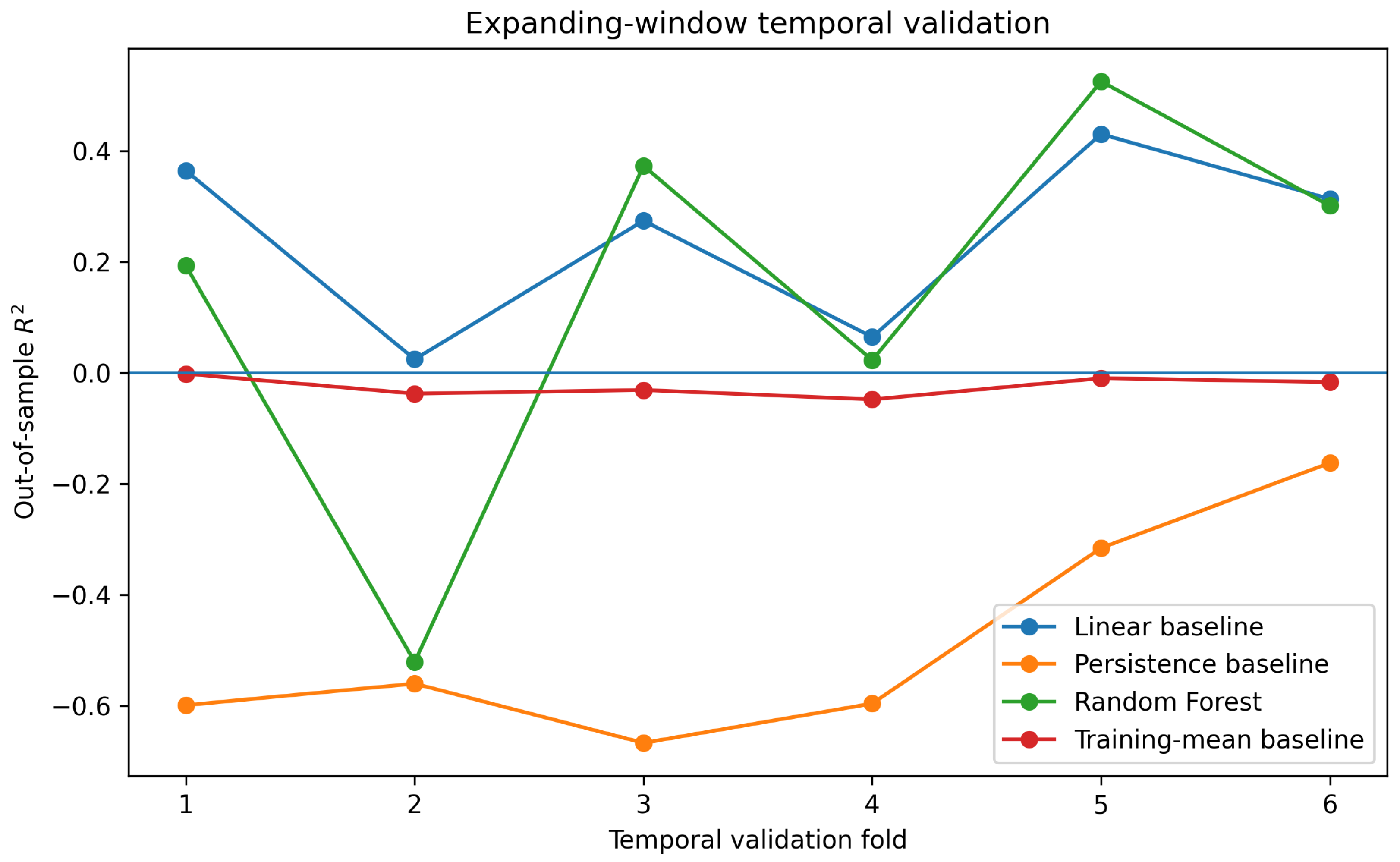
Expanding-window validation materially changed the interpretation of the RF. Mean out-of-sample $R^2$ was 0.149, with RMSE 0.913 and MAE 0.656 (

Table 3. Expanding-window predictive performance averaged across six temporal folds.

Model	Mean ${\mathit{R}}^2$	Mean RMSE	Mean MAE
Random Forest	0.149	0.913	0.656
Linear baseline	0.246	0.890	0.628
Persistence baseline	$-0.483$	1.247	0.832
Training-mean baseline	$-0.024$	1.051	0.785

). A linear baseline using the same current-month predictors performed better on average ($R^2=0.246$, RMSE 0.890, MAE 0.628), while persistence and training-mean baselines had negative mean $R^2$. Held-out permutation importance was largest for LST (0.104) and precipitation (0.099), followed by soil moisture (0.036), NDVI (0.016), and ET ($-0.008$). Soil-moisture importance was positive in all six folds; LST and precipitation were positive in five of six. Figure 2 shows foldwise performance and therefore supports retaining RF as a conditional nonlinear attribution sensitivity, not as evidence that a complex nonlinear model forecasts fire better than a simple baseline.

3.3. H1: Short-Horizon Surface State

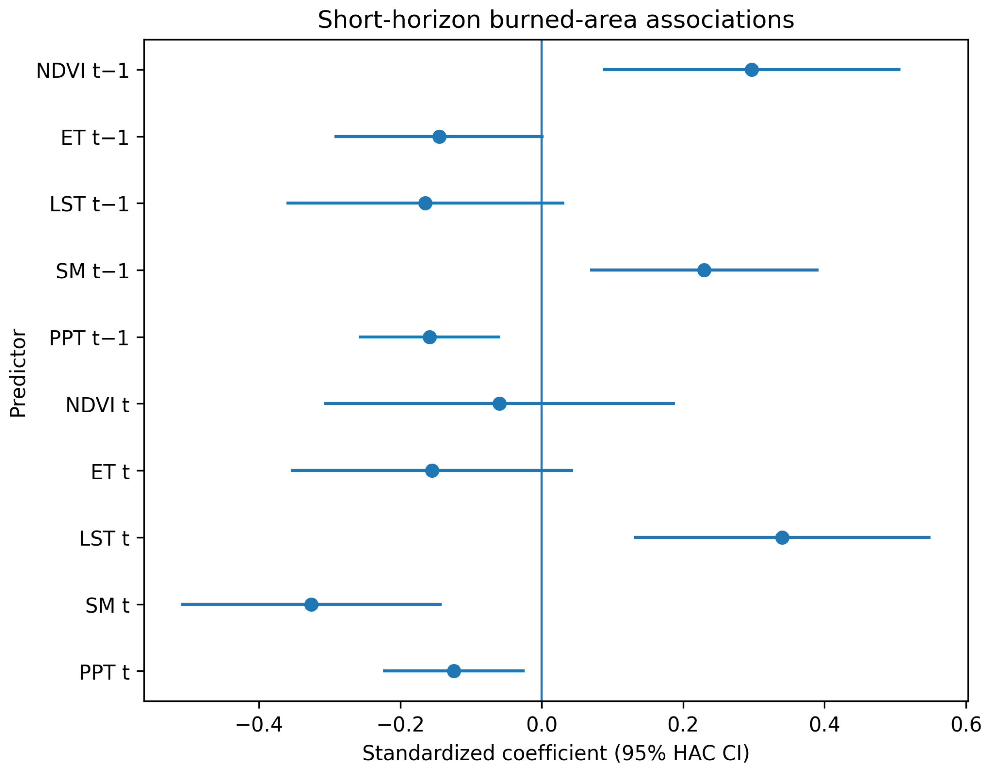
The H1 HAC model supported the expected current-month surface-state signs (

Table 4. Selected coefficients from the H1 short-horizon HAC regression.

Term	$\mathit{\beta }$	HAC SE	p
Burned area $t-1$	0.213	0.062	0.0006
Precipitation t	$-0.124$	0.051	0.0149
Soil moisture t	$-0.326$	0.094	0.0005
Daytime LST t	0.340	0.107	0.0015
ET t	$-0.155$	0.102	0.1272
NDVI t	$-0.060$	0.127	0.6373
Precipitation $t-1$	$-0.159$	0.051	0.0019
Soil moisture $t-1$	0.230	0.082	0.0052
LST $t-1$	$-0.165$	0.100	0.1006
ET $t-1$	$-0.145$	0.075	0.0544
NDVI $t-1$	0.297	0.107	0.0057

and Figure 3). Daytime LST was positively associated with burned-area anomaly ($\beta =0.340$, $p=0.0015$), whereas near-surface soil moisture was negatively associated ($\beta =-0.326$, $p=0.0005$). Current precipitation was also negative ($\beta =-0.124$, $p=0.0149$). The one-month soil-moisture coefficient reversed sign ($\beta =0.230$, $p=0.0052$), demonstrating why soil moisture should not be assigned a single mechanistic sign across time scales.

The LST coefficient remained positive and significant after ERA5-Land precipitation and/or soil-moisture substitution, persistent-cropland NDVI substitution, and exclusion of months with low daytime-LST coverage. The current soil-moisture coefficient remained negative in every product specification, although it was not significant when both precipitation and soil moisture were simultaneously replaced by ERA5-Land. H1 is therefore supported as a short-horizon surface-state association, not as proof of an independent thermal causal effect or direct fuel-moisture mechanism.

3.4. H2: Antecedent Hydroclimatic History

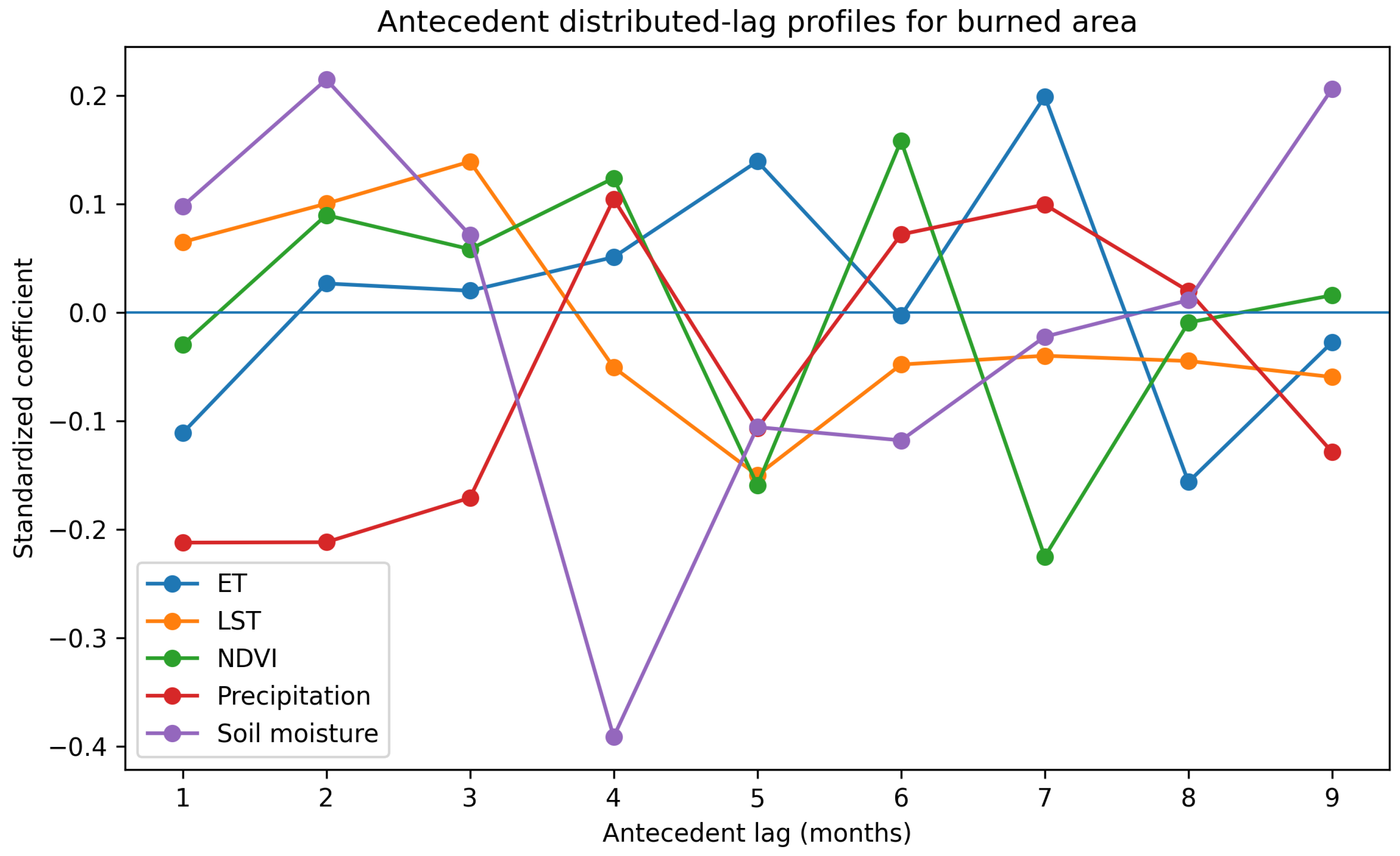
The dedicated 1–9 month distributed-lag model yielded strong joint evidence for precipitation and soil-moisture history (

Table 5. H2 joint 1–9 month lag-block tests with BH-FDR correction.

Predictor History	F	p	${\mathit{q}}_{\mathbf{BH}}$
Precipitation	5.271	$1.81\times {10}^{-6}$	$9.03\times {10}^{-6}$
Near-surface soil moisture	3.407	0.000630	0.001576
Daytime LST	1.205	0.293	0.451
ET	1.104	0.361	0.451
NDVI	0.417	0.925	0.925

FDR-surviving individual lags: precipitation L1 $\beta =-0.212$ ($q=0.0400$); precipitation L2 $\beta =-0.212$ ($q=0.0071$); soil moisture L4 $\beta =-0.391$ ($q=0.0398$). Complete 45-lag results are provided in Supplementary Table S7.

and Figure 4). After BH-FDR correction across predictor blocks, precipitation remained strongly supported ($F=5.271$, $q=9.03\times {10}^{-6}$) and soil moisture was also supported ($F=3.407$, $q=0.0016$). In contrast, the joint histories of LST ($q=0.451$), ET ($q=0.451$), and basin-wide NDVI ($q=0.925$) were not supported.

Multiplicity control substantially reduced the number of interpretable individual lags. Of 45 predictor-lag coefficients, only precipitation at one month ($\beta =-0.212$, $q=0.0400$), precipitation at two months ($\beta =-0.212$, $q=0.0071$), and soil moisture at four months ($\beta =-0.391$, $q=0.0398$) survived BH-FDR. The negative precipitation result was robust to ERA5-Land substitution. Soil-moisture history remained significant in most product configurations but weakened when ERA5 precipitation was paired with GLDAS soil moisture. Persistent-cropland NDVI had a significant joint lag block in sensitivity analysis, but basin-wide NDVI did not; this isolated sensitivity is insufficient to support a general basin-wide fuel-accumulation claim.

3.5. VAR Specification and Reduced-Form Dynamics

The lag diagnostics do not support VAR(9) as a unique or preferred specification (

Table 6. Selected VAR lag-order and diagnostic results. Information criteria are calculated on the common 251-month comparison sample used for lag selection; residual degrees of freedom and whiteness tests are from the corresponding order-specific fitted models.

Lag	Coef./Eq.	System Coef.	Residual df	AIC	BIC	FPE	HQIC	Whiteness p
1	7	42	255	$-5.390$	$-4.800$	0.004561	$-5.153$	$8.48\times {10}^{-9}$
4	25	150	234	$-5.471$	$-3.365$	0.004222	$-4.624$	0.00404
9	55	330	199	$-5.305$	$-0.670$	0.005187	$-3.440$	$1.45\times {10}^{-7}$

BIC/HQIC select lag 1; AIC/FPE select lag 4. System whiteness rejects at every tested lag order, motivating secondary rather than primary use of VAR inference.

). On the common 251-month comparison sample, BIC and HQIC selected VAR(1), whereas AIC and FPE selected VAR(4). VAR(9) estimates 55 coefficients per equation (330 system coefficients) and leaves 199 residual degrees of freedom per equation; VAR(4) estimates 25 coefficients per equation (150 system coefficients) and leaves 234 residual degrees of freedom. All orders through nine lags were companion-matrix stable, but the multivariate residual-whiteness test rejected at every order. For VAR(4), equation-level Ljung–Box tests did not reject residual autocorrelation, although ARCH effects remained for NDVI and precipitation and normality was rejected for burned area, NDVI, and precipitation.

Joint predictive-precedence tests were more stable than individual VAR coefficients. Precipitation history improved prediction of burned area after BH-FDR at VAR(1) ($q=0.0145$), VAR(4) ($q=0.000855$), and VAR(9) ($q=0.00935$); no individual non-self lag in the VAR(9) burned-area equation survived FDR. Generalized VAR(4) impulse responses and Cholesky-order sensitivity are therefore presented in the Supplement rather than used as primary H1–H3 evidence.

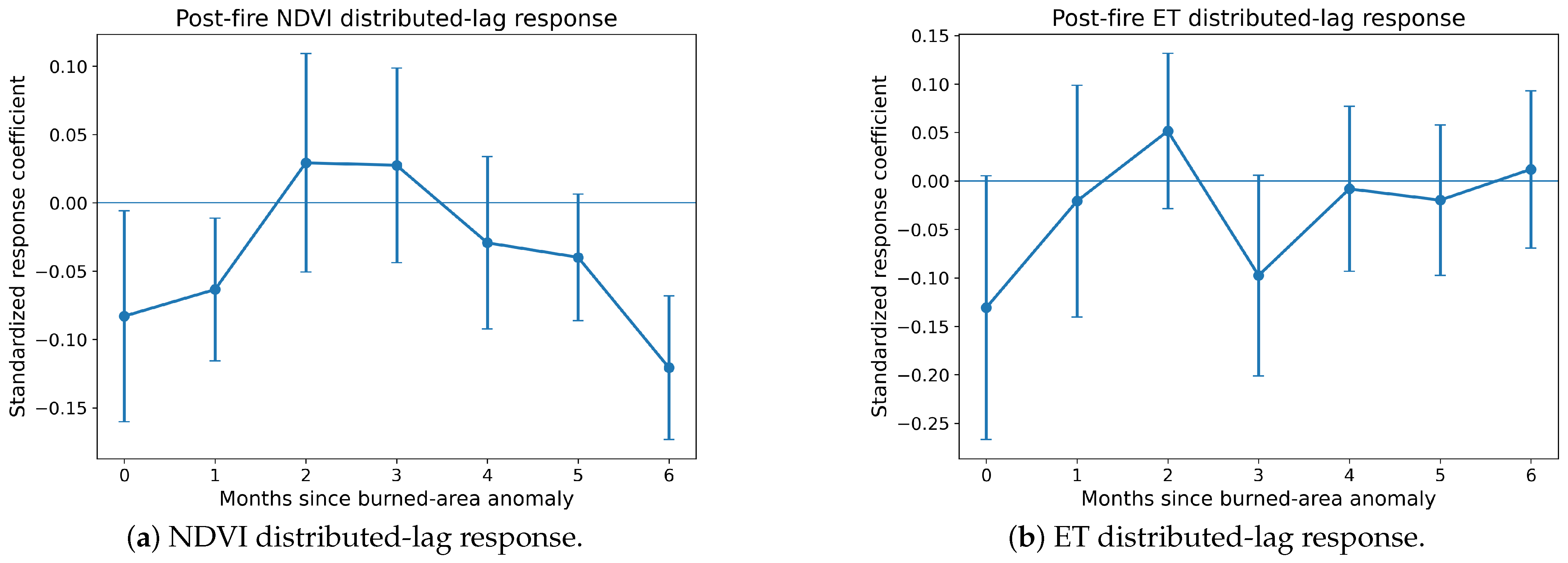
3.6. H3: Post-Fire Vegetation and Water-Flux Response

Burned-area history was associated with a delayed basin-wide NDVI response after adjustment for NDVI persistence and concurrent hydroclimate (

Table 7. Primary and lag-window sensitivity results for H3.

Outcome	Window	Joint p	Cumulative $\mathit{\beta }$	95% CI Low	95% CI High
NDVI	0–3 months	0.266	$-0.028$	$-0.137$	0.080
NDVI	0–6 months	$1.05\times {10}^{-5}$	$-0.280$	$-0.452$	$-0.107$
NDVI	0–9 months	$2.40\times {10}^{-7}$	$-0.323$	$-0.519$	$-0.128$
ET	0–3 months	0.00738	$-0.196$	$-0.352$	$-0.040$
ET	0–6 months	0.0175	$-0.214$	$-0.419$	$-0.008$
ET	0–9 months	0.00756	$-0.178$	$-0.423$	0.068

Future-burn placebo $p=0.740$ for NDVI and $p=0.061$ for ET in the 0–6 month specification.

and Figure 5). The 0–6 month burn-lag block was jointly significant ($F=5.343$, $p=1.05\times {10}^{-5}$), with cumulative standardized effect $\Theta =-0.280$ (95% CI $[-0.452,-0.107]$). A future-burn placebo was null ($p=0.740$). The cumulative 0–3 month interval crossed zero, whereas 0–6 and 0–9 month intervals were negative, indicating a delayed rather than immediate net greenness response. The result remained negative under alternate precipitation and soil-moisture controls; persistent-cropland NDVI did not show a cumulative interval excluding zero.

ET also declined following high burned-area anomalies. The 0–6 month burn-lag block was significant ($F=2.487$, $p=0.0175$), with cumulative effect $\Theta =-0.214$ (95% CI $[-0.419,-0.008]$). The future-burn placebo exceeded the 0.05 threshold but was comparatively close ($p=0.061$), warranting more caution than for NDVI. ET cumulative effects were negative over 0–3 and 0–6 months, while the 0–9 month interval crossed zero. The evidence therefore supports a short-to-intermediate post-fire ET reduction, not a persistent long-term hydrologic-memory claim.

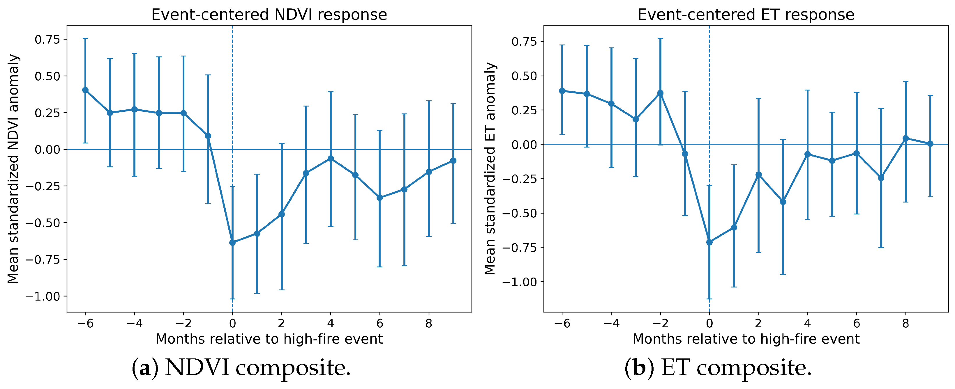
3.7. Event-Centered Descriptive Check

The 90th-percentile rule identified 27 candidate high-fire months; grouping consecutive candidates into contiguous episodes and retaining the maximum-burn month from each episode yielded 20 declustered events. Mean NDVI and ET anomalies were negative in the event month and the following month, with bootstrap intervals below zero at the shortest horizons, but intervals widened and generally crossed zero later. Figure 6 is therefore used as descriptive corroboration only; it does not identify a fire treatment effect and does not replace the controlled distributed-lag models.

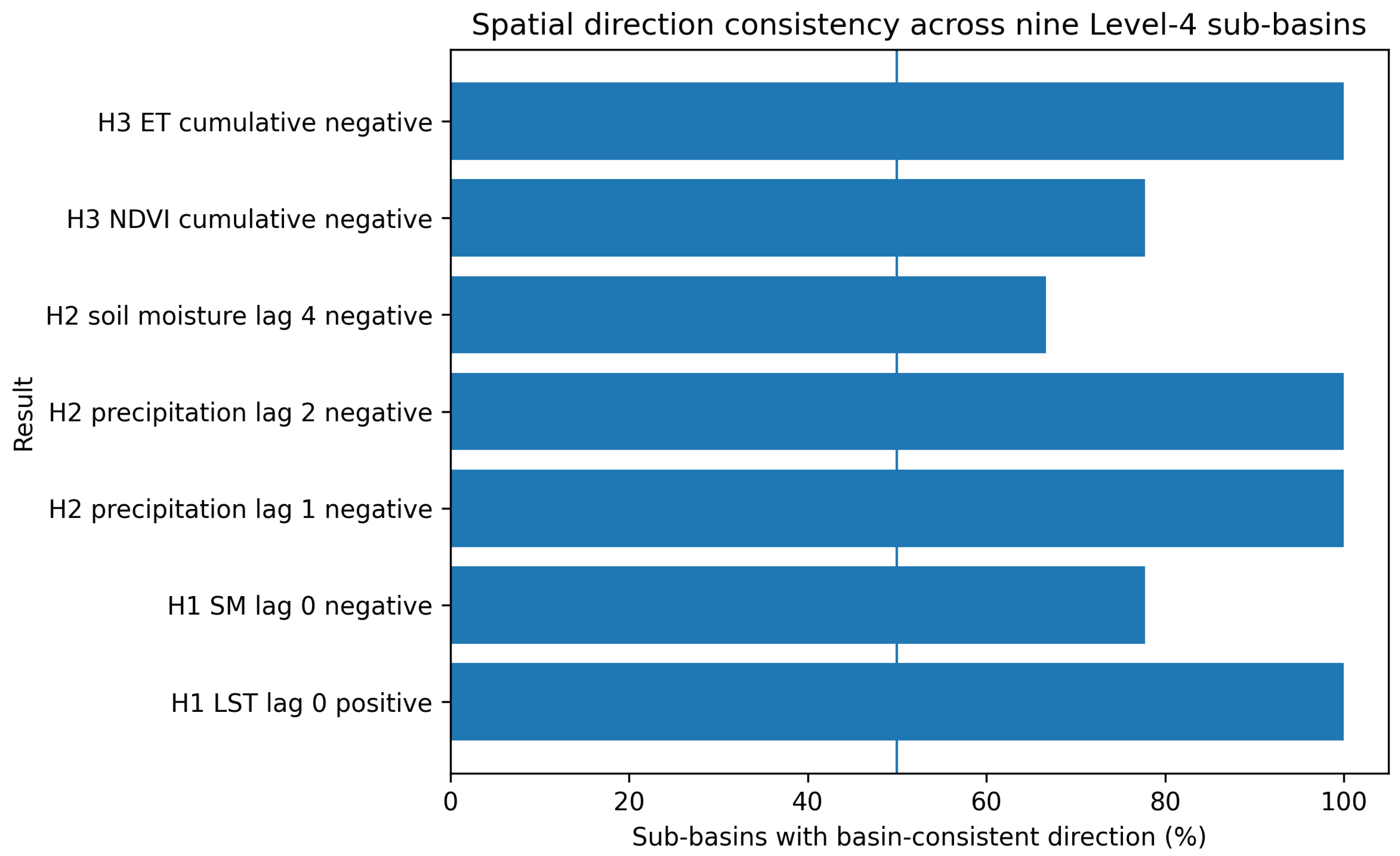
3.8. Spatial Robustness Across Level-4 Sub-Basins

The basin-scale results were not solely artifacts of one spatial average, although the strength of evidence varied among sub-basins (

Table 8. Direction consistency across nine Level-4 HydroBASINS units.

Result	Expected Direction	Units Consistent	Nominally Significant in Direction
H1 LST lag 0	Positive	9/9	8/9
H1 soil moisture lag 0	Negative	7/9	5/9
H2 precipitation lag 1	Negative	9/9	6/9
H2 precipitation lag 2	Negative	9/9	2/9
H2 soil moisture lag 4	Negative	6/9	2/9
H3 NDVI cumulative	Negative	7/9	3/9
H3 ET cumulative	Negative	9/9	3/9

and Figure 7). The current LST coefficient was positive in all nine units and nominally significant in eight. Current near-surface soil moisture was negative in seven of nine. Precipitation coefficients at one and two months were negative in all nine units; the four-month soil-moisture coefficient was negative in six. The cumulative NDVI response was negative in seven of nine units, with three 95% intervals fully below zero. The cumulative ET response was negative in all nine units, also with three intervals fully below zero. The appropriate conclusion is therefore directional basin-scale support with genuine spatial heterogeneity, not spatial uniformity.

4. Discussion

4.1. Evidence Supported by the Analysis

The results support a deliberately constrained interpretation of the Zambezi fire–hydroclimate system. The strongest result is a short-horizon surface-state association: warmer daytime LST and lower near-surface soil moisture coincide with larger burned-area anomalies after adjustment for burned-area persistence and correlated current/lagged land-surface variables. The LST sign is robust to alternate precipitation and soil-moisture products, cropland-NDVI substitution, and removal of low-LST-coverage months, and it is positive in all nine Level-4 sub-basins. This pattern is consistent with near-term surface heating and drying, but the statistical model does not isolate an autonomous thermal mechanism. LST integrates radiation, vegetation, surface moisture, and turbulent exchange, and its coefficient should be read as an integrated surface-state signal rather than as a causal air-temperature effect [10,11].

The antecedent analysis provides a second, distinct result: precipitation and near-surface soil-moisture histories retain joint 1–9 month information about burned-area anomalies after FDR control. The FDR-surviving precipitation coefficients at one and two months and the soil-moisture coefficient at four months are negative, and precipitation L1–L2 signs are negative in all nine sub-basins. These timings are physically consistent with delayed moisture suppression in seasonal savannas, but the mechanism is not uniquely identified. Precipitation, soil moisture, vegetation activity, humidity, VPD, and human burning are coupled; the observed coefficients establish temporal conditional associations, not a controlled moisture pathway.

In contrast, the basin-wide results do not support antecedent NDVI as robust evidence of fuel accumulation. The joint basin-wide NDVI lag block is not significant after FDR, nor are ET or LST histories independently supported over 1–9 months. Cropland-only NDVI becomes significant in one sensitivity specification, which is scientifically interesting but insufficient to generalize a basin-wide fuel-production mechanism. NDVI is optical greenness and does not directly quantify fuel load, continuity, curing, or vegetation water content [15,17,46]. The interpretation therefore distinguishes measured vegetation greenness from hypothesized fuel properties.

The post-fire analysis supports a more specific interpretation than a broad “memory” framing. Basin-wide NDVI exhibits a delayed cumulative decline over 0–6 and 0–9 months, with a null future-burn placebo and robustness to alternate hydroclimate controls. ET shows a shorter-lived negative cumulative response over 0–3 and 0–6 months but the 0–9 month CI crosses zero and the future-burn placebo is borderline. These results support post-fire vegetation and water-flux response, not persistent ecosystem degradation or long-term hydrologic memory. The spatial analysis reinforces this qualification: NDVI and ET directions are often shared across sub-basins, but only a minority of units have cumulative intervals fully below zero.

4.2. Random Forest and Correlated Predictors

Temporal validation removes a potential source of overstatement. The RF does not outperform the linear baseline on average, even though its held-out permutation importance identifies LST and precipitation as the largest contributors and finds positive soil-moisture importance in every fold. This outcome is informative because it shows that nonlinear attribution is not synonymous with superior forecasting. The moderate correlations among predictors, especially ET–NDVI and LST–NDVI, further imply that any feature-importance ranking is conditional on the included predictor set. The VIFs are not large enough to imply extreme linear collinearity, but they do not solve attribution ambiguity in nonlinear models. We therefore use RF only as a sensitivity analysis and give inferential priority to explicitly specified HAC regressions.

4.3. VAR Diagnostics and the Limits of Predictive Precedence

The VAR diagnostics show the consequences of overparameterization and multiple testing. Common-sample information criteria do not select nine months uniformly: BIC and HQIC favor one lag, while AIC and FPE favor four. VAR(9) estimates 330 system coefficients from a 263-month record and leaves 199 residual degrees of freedom per equation. Although fitted systems through nine lags are stable, the multivariate whiteness test rejects at every order. This failure matters because it weakens the usual interpretation of standard VAR innovations and impulse responses. Equation-level diagnostics are less severe for VAR(4), but ARCH effects and non-normality remain in several equations.

For that reason, the VAR no longer carries the main inferential burden. Joint predictive-precedence tests consistently identify precipitation history, but individual VAR(9) lag coefficients do not survive FDR. GIRFs and multiple Cholesky orderings are retained as secondary descriptions of reduced-form propagation only. This is consistent with the broader distinction between temporal prediction and structural causality emphasized in time-series methodology [21,22].

4.4. Spatial Scale, Product Resolution, and Hydrological Interpretation

The Level-4 analysis confirms that several basin-scale directions are geographically widespread, especially current LST, lagged precipitation, and cumulative ET response. At the same time, effect magnitude and significance vary substantially among sub-basins. The Zambezi spans hydroclimatic, vegetation, topographic, and land-use gradients; a single basin-average series cannot resolve all local processes. We therefore limit the conclusions to basin-integrated and major-sub-basin temporal associations.

Spatial-resolution mismatch is handled by native-grid area weighting rather than common-grid upsampling. This preserves the information content of each product but does not remove representativeness uncertainty: a coarse hydroclimatic pixel and a 500-m fire pixel describe different spatial supports. Likewise, the primary GLDAS 0–10 cm soil-moisture series and ERA5-Land 0–7 cm sensitivity are near-surface model/reanalysis variables. Neither is vegetation-accessible root-zone water, live-fuel moisture, or vegetation water content. Those distinctions are particularly important in savannas, where deep-rooted woody vegetation and shallow grass fuels can experience different water constraints [47,48].

Published validation provides context but not basin-specific truth. CHIRPS has demonstrated useful monthly skill in African gauge comparisons while retaining regional and elevation-dependent biases [38,39]. ERA5-Land’s surface soil moisture has also been evaluated against in situ networks, including African sites, but product uncertainty remains [36]. Cross-product agreement in the present study increases confidence that the principal precipitation result is not tied to one dataset; the more modest soil-moisture agreement is consistent with its greater product sensitivity.

4.5. Alternative Explanations and Causal Limits

The statistical models omit important determinants of savanna fire: vapor pressure deficit, relative humidity, wind speed and direction, lightning, human ignition, agricultural burning, grazing, land-cover conversion, roads and accessibility, fire suppression, and local fire-management practices. Several of these factors can influence both the predictors and burned area. Human activity is known to alter African fire regimes substantially [5,49], while atmospheric fire weather can affect ignition and spread independently of the land-surface variables included here [50,51]. These omissions prevent unique mechanistic attribution.

Accordingly, terms such as moisture suppression, fuel accumulation, and recovery are used only as physical interpretations consistent with observed signs and timing. The analysis establishes conditional temporal association, robustness across data products and spatial units, and predictive precedence in limited secondary models. It does not estimate a causal effect of LST, soil moisture, precipitation, NDVI, ET, or burned area under a fully identified intervention.

4.6. Implications

The practical implication is that seasonal fire assessment should preserve time scale and measurement meaning. Current surface thermal and moisture states contain information distinct from antecedent hydroclimatic histories; post-fire NDVI and ET responses occur on yet another horizon. Models that collapse these variables into one contemporaneous ranking can obscure this structure. At the same time, complexity should be justified by temporal generalization: in this dataset, a linear baseline predicts future holdout blocks better on average than the RF.

For multi-source environmental fire studies more broadly, these analyses illustrate a reproducible workflow: define hypotheses in terms of measured variables and lag windows; avoid common-grid upsampling when native resolution is adequate for regional aggregation; export valid-area coverage; validate machine learning chronologically; report full lag results with multiplicity correction; diagnose high-order time-series systems; include cumulative confidence intervals and placebos for post-disturbance models; and test whether basin-average signs persist across meaningful spatial units.

5. Conclusions

Using a quality-audited 263-month multi-source environmental record, we identify three principal results. First, burned-area anomalies are larger during months with warmer daytime LST and lower near-surface soil moisture; these are robust short-horizon surface-state associations, not independently identified causal mechanisms. Second, precipitation and near-surface soil-moisture histories contain significant 1–9 month information about burned area after FDR correction, with negative precipitation L1–L2 and soil-moisture L4 coefficients consistent with delayed wetness-related suppression. Basin-wide NDVI, ET, and LST histories do not provide independent joint evidence over the same window. Third, burned-area history is followed by a delayed basin-wide NDVI decline and a shorter-lived ET reduction, supporting post-fire vegetation and water-flux response while not establishing persistent ecosystem “memory.”

The Level-4 analysis shows that the principal LST, precipitation, and ET directions are geographically widespread, but effect magnitude and certainty vary among sub-basins. Random Forest temporal validation and VAR diagnostics further constrain interpretation: the RF does not outperform a linear baseline, and residual-whiteness failures require VAR/impulse-response results to remain secondary. Taken together, the evidence favors a cautious, time-scale-specific description of wildfire–vegetation–water coupling in the Zambezi Basin.