M-FSAD-KD: Full-Link Multi-Granularity Distillation for SAR Object Detection

Highlights

What are the main findings?

• A “speckle-fitting trap” is identified: channel-wise feature distillation pushes a SAR-only student below its non-distilled baseline, collapsing small-target accuracy.
• A Fourier low-pass mask is repurposed as a gate on the distillation loss—transferring low-frequency structure while leaving the student’s target-edge high-frequency band free.

What are the implications of the main findings?

• The full-link feature-distillation chain (M-FSAD-KD) matches response-level KD on a 2.39 M student and surpasses it by 2.0 mAP50 on a 19.98 M student.
• Frozen-feature transfer to an out-of-domain SAR benchmark (SSDD) shows the distilled features are the most transferable among all compared methods.

Abstract

Multi-modal synthetic aperture radar (SAR)–optical object detectors raise detection accuracy by fusing complementary physical responses, but require both modalities to be simultaneously available at inference. When the optical stream becomes unavailable—under heavy cloud cover, night-time conditions, or downlink disruption—the detector reverts to SAR-only operation and accuracy degrades sharply. A natural remedy is to distil a multi-modal teacher into a SAR-only student via privileged-information knowledge distillation. However, we observe that the leading channel-wise feature-level method (CWD) reduces the student’s accuracy below the non-distilled baseline, with its smallest-target AP collapsing to near zero, because SAR speckle and target high-frequency edges share the same band and the alignment loss is dominated by broadband speckle energy. We refer to this failure mode as the speckle-fitting trap, formalize it as a gradient-pollution effect, and validate it through spectral and feature-manifold diagnostics. To counter the trap, we propose M-FSAD-KD, a full-link distillation framework whose neck-stage Fourier-gated alignment transfers low-frequency structural content while preserving target-edge high-frequency content; a joint spatial–channel attention mask, a shallow backbone adapter, and a response-level knowledge distillation (KD) term complete the chain. With a MAIENet teacher on OGSOD-1.0, the advantage of M-FSAD-KD over the strongest response-level KD baseline scales with student capacity: it matches KD on a 2.39 M-parameter student (both ≈48% mean average precision at an intersection-over-union (IoU) threshold of 0.5 (${\mathrm{mAP}}_{50}$), averaged over multiple seeds) and exceeds it by 2.0 absolute points on a 19.98 M-parameter student ($+8$ over the non-distilled baseline), where it is the best of all distillation methods; at full convergence the 19.98 M-parameter student reaches 81.9% ${\mathrm{mAP}}_{50}$, within 8.9 absolute points of the multi-modal teacher. A frozen-feature transfer test to an out-of-domain SAR benchmark (SSDD ship detection) further shows that distilling from the multi-modal teacher yields substantially more transferable SAR features—about ten absolute points above the non-distilled backbone—with M-FSAD-KD transferring best. Cross-architecture validation with a dual-stream DEYOLO teacher yields 48.6% ${\mathrm{mAP}}_{50}$ at the student—1.1 absolute points below the MAIENet result—indicating that the framework transfers across the two representative teacher architectures tested (single-stream and dual-stream).

1. Introduction

Synthetic aperture radar (SAR) provides all-weather, day-and-night observation by actively transmitting coherent microwave pulses and recording the back-scattered echoes [1]. The coherent imaging mechanism, however, imprints a multiplicative non-Gaussian speckle noise on every pixel, and the SAR signal lacks the continuous reflectance spectra and texture geometry available from the optical band. In coastal and cluttered industrial backgrounds, the discrete scattering centers of small targets such as bridges, harbors, and oil tanks become statistically difficult to distinguish from speckle clutter, and the separability between target and clutter in the deep feature space degrades [2,3].

To break this single-band ceiling, recent works [4,5] register high-resolution optical imagery to the SAR scene and design multi-modal SAR–optical detectors. In a concurrent line of our own work [6], we proposed MAIENet, a single-stream modality-aware interaction enhancement network that exploits both microwave back-scatter and optical reflectance through deformable cross-modal alignment at the deepest semantic stage and attains  90.8% mean average precision at an intersection-over-union (IoU) threshold of 0.5 (${\mathrm{mAP}}_{50}$) on the OGSOD-1.0 benchmark at a parameter budget below conventional two-stream baselines. When both modalities remain available, such detectors substantially raise the upper bound of detection accuracy.

The assumption of complete modality availability is brittle in practice. Optical sensors fail under heavy cloud cover, dense aerosols, or night-time low illumination, and the synchronized downlink delivering paired SAR–optical samples is vulnerable to disruption. When inference is forced down to a single SAR stream, the deep feature manifold—trained under the joint distribution—suffers a structural mismatch, and detection performance can drop by tens of absolute points [7,8].

Knowledge distillation (KD) under the Learning-Using-Privileged-Information (LUPI) framework [9,10,11] offers a structured remedy: a multi-modal teacher is trained with both SAR and optical inputs, and its knowledge is distilled into a lightweight SAR-only student that operates alone at inference. Direct transfer is, however, impeded by a physical mismatch. The intermediate features of the multi-modal teacher couple optical texture with microwave back-scattering parameters; forcing the low-capacity SAR student to match this heterogeneous representation directly under a Euclidean criterion induces semantic drift. In addition, SAR speckle appears in the student’s hidden features as a broadband, high-frequency random perturbation. Conventional distance-based or spatial-mask distillation losses then cause the optimizer to spend its limited gradient budget on fitting the speckle pattern, as we confirm empirically in Section 4. We refer to this phenomenon as the speckle-fitting trap: the student exhausts its representational capacity on noise that carries no semantic content, narrowing its generalization margin and raising its false-alarm rate. Response-level distillation alone is insufficient to remedy this failure mode, because the student then lacks the intermediate feature representation required to recover the missing optical prior [12].

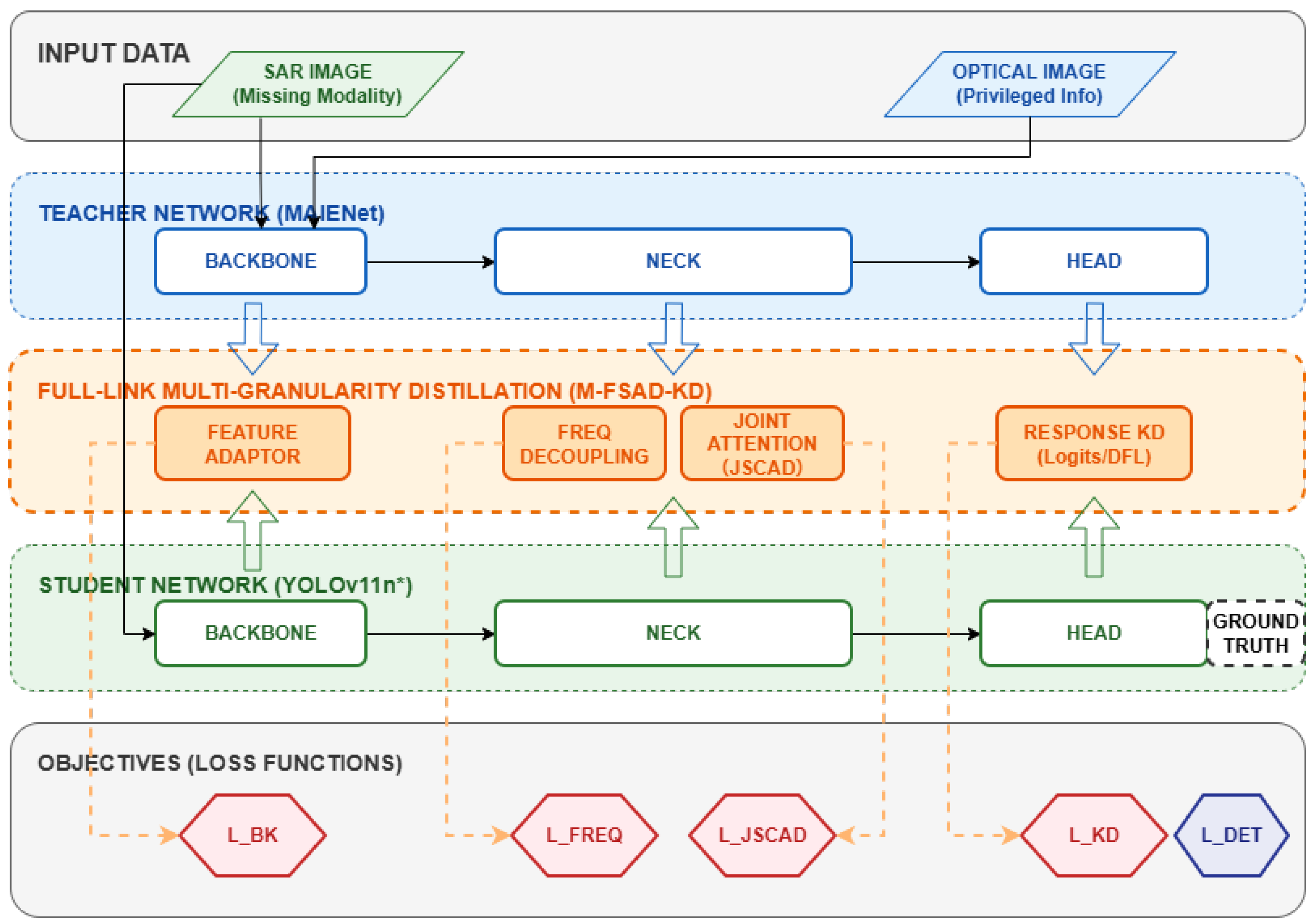
This paper addresses the speckle-fitting trap with an architectural response rather than a single new loss term. We propose M-FSAD-KD (Multi-granularity Frequency-and-Spatial-Attention Distillation with head Knowledge Distillation), a full-link distillation framework that refines SAR-only student features through four complementary granularities arranged along the student’s network depth. At the shallow backbone level, a learnable adapter (Bk) projects the student feature onto the teacher’s channel-aligned representation so that subsequent alignment losses are geometrically well-posed. At the neck stage, frequency-decoupled distillation (Freq) gates the teacher–student amplitude-spectrum alignment via a dynamic Gaussian low-pass mask, transferring the low-frequency structural information while leaving the high-frequency band free for the SAR-only student to retain its own target-edge content required for small-object localization. Co-located at the same stage, joint spatial–channel attention distillation (JSCAD) modulates the alignment loss with a three-dimensional mask derived from the teacher’s spatial saliency and channel discriminability, directing the gradient toward high-entropy regions. At the head end, a response-level term (KD) calibrates the soft decision boundary over the purified feature manifold. The four components are coordinated by a dimensional-homogenization weight scheme that maintains comparable gradient magnitudes throughout training.

The framework transfers across the two teacher architectures we test—a single-stream (MAIENet) and a two-stream (DEYOLO [13]) multi-modal SAR–optical detector, as validated in Section 4.4.2; we do not claim architecture-agnosticism beyond these two families. We adopt MAIENet [6] as the primary teacher because it offers high accuracy at a controlled parameter budget on the same benchmark used for student evaluation. The teacher is treated as a black-box input; the contribution of this paper lies in the distillation framework and the diagnosis of the speckle-fitting trap.

The principal contributions of the paper are summarized as follows.

• We characterize the speckle-fitting trap in cross-modal SAR distillation and provide two lines of evidence for it: empirical evidence (the degradation of CWD below the non-distilled baseline) and physical evidence (frequency-domain spectral analysis together with a formal gradient-pollution argument).
• We propose frequency-decoupled distillation (Freq), a neck-stage component that gates the teacher–student amplitude-spectrum alignment through a dynamic Gaussian low-pass mask defined in the 2D Fourier domain. To our knowledge, this is the first formulation that repurposes a Fourier low-pass filter as a knowledge-transfer gate within the distillation loss for cross-modal SAR detection.
• We propose joint spatial–channel attention distillation (JSCAD), a 3D-tensor mask formed by the outer product of the teacher’s spatial saliency and channel discriminability, which directs the alignment gradient toward high-entropy semantic regions while preserving channel separability.
• We integrate Bk, Freq, JSCAD, and a response-level KD term into a full-link framework with a dimensional-homogenization loss-weight calibration. The framework consistently improves SAR-only detection across student capacities of 2.39 M and 19.98 M parameters on OGSOD-1.0, and transfers across teacher architecture families (validated on single-stream MAIENet and dual-stream DEYOLO).

The remainder of this paper is organized as follows. Section 2 reviews related work. Section 3 details the proposed framework. Section 4 reports the experimental analysis. Section 5 discusses observations and limitations. Section 6 concludes the work.

2. Related Work

2.1. Multi-Modal SAR–Optical Object Detection

Multi-modal SAR–optical detectors overcome the single-band separability ceiling by fusing complementary physical responses. Cross-modal knowledge distillation methods such as CoLD [5] treat optical features as privileged knowledge and inject them unidirectionally into a SAR detector. Two-stream feature-level fusion methods—DEYOLO [13], CMADet [14], ICAFusion [15], and CSSA [16]—maintain parallel feature extractors and perform channel modulation or spatial cross-attention at intermediate depths. Single-stream alternatives such as MAIENet [6], which we proposed in concurrent work, share a single backbone and perform modality-aware interaction at the deepest semantic stage, mitigating the parameter explosion of two-stream architectures. None of these methods are designed to operate when one of the two modalities is absent at inference; their robustness under modality dropout is an orthogonal question, which the present paper addresses through privileged-information distillation rather than fusion.

2.2. Knowledge Distillation for Object Detection

Logits-level knowledge distillation [11,17] transfers dark knowledge through softened class distributions. For dense detection, feature-level distillation has proved indispensable [12]: FitNet [18] aligns intermediate feature maps via pixel-wise MSE; FGD [19] introduces focal and global masks derived from teacher activations; MGD [20] performs masked feature reconstruction; LD [21] adapts logit distillation to the localization branch; DKD [22] decouples target-class from non-target-class distillation; CWD [23] aligns channel-wise softmaxed distributions and GID [24] performs instance-aware filtering before alignment. These methods implicitly assume that the teacher and student share a quasi-homogeneous feature manifold. The assumption breaks down across heterogeneous modalities such as SAR and optical—the regime addressed in this paper—and gives rise to the speckle-fitting trap diagnosed in Section 3.8.

2.3. Privileged Information and Missing-Modality Robustness

Cross-modal distillation extends the LUPI framework of Vapnik et al. [9]. Gupta et al. [10] generalize LUPI to feature distillation across modalities, demonstrating that an RGB-only student can approximate the accuracy of an RGB-D teacher. In remote sensing, Wei et al. [8] propose MMANet for complementary information modeling under modality dropout; Li et al. [7] comprehensively review deep-learning fusion of multimodal remote-sensing data and note that robustness under incomplete or degraded modalities remains an open challenge; and even the SAR-specific cross-modal distillation of CoLD [5] aligns the optical and SAR detectors purely in the spatial domain. None of these works directly addresses the spectral overlap between SAR speckle and target high-frequency content, which we identify as the root cause of the speckle-fitting trap.

2.4. Frequency-Domain Learning

Frequency-domain mechanisms have been deployed in vision at three loci: as backbone operators that modulate the forward computation [25], as masked self-supervised pretraining objectives [26], and as distillation-channel aligners that reshape feature distributions [23]. All three inject frequency information at the operator level. By contrast, M-FSAD-KD repurposes a Fourier low-pass filter as a knowledge-transfer gate on the distillation loss while leaving the forward operators of both teacher and student unchanged. To our knowledge, this loss-gating role is new in cross-modal SAR detection and is the operative reason the framework avoids the speckle-fitting trap.

3. Methodology

3.1. Problem Setting and Notation

Let the multi-modal training set be ${\mathcal{D}}_{\mathrm{train}}={\left\{({\mathbf{x}}_s^i,{\mathbf{x}}_o^i,y^i)\right\}}_{i=1}^N$, where ${\mathbf{x}}_s^i\in {\mathbb{R}}^{1\times H\times W}$ is a single-channel SAR amplitude image, ${\mathbf{x}}_o^i\in {\mathbb{R}}^{3\times H\times W}$ is a spatially co-registered optical image, and $y^i$ contains the ground-truth bounding boxes and class labels. The teacher network $T(·,·)$ ingests the paired input $({\mathbf{x}}_s,{\mathbf{x}}_o)$ and produces the privileged features ${\mathbf{F}}_T$. The student network $S(·)$ ingests only ${\mathbf{x}}_s$ and produces the features ${\mathbf{F}}_S$. All distillation components (adapters, masks, and auxiliary losses) are active only during training and are removed at inference time, so that the deployed student receives no optical input and incurs no distillation-related cost.

To address the heterogeneous-modality gap and the semantic drift induced by direct Euclidean alignment between the multi-modal teacher manifold and the SAR-only student manifold, we propose the full-link M-FSAD-KD framework (Figure 1). Four granularities operate jointly during training: shallow backbone adaptation (Bk), frequency-decoupled distillation (Freq), joint spatial–channel attention distillation (JSCAD), and end-stage response distillation (KD).

3.2. Shallow Backbone Adaptation (Bk)

The teacher’s shallow activations integrate optical texture by construction, whereas the student observes only microwave back-scatter; the two feature spaces, therefore, differ in both channel count and statistical support. To restore a geometrically well-posed alignment target, we introduce a per-layer adapter $\varphi (·)$ that projects the student feature into the teacher’s channel space:

$${\widehat{\mathbf{F}}}_{S,l}=\varphi \left({\mathbf{F}}_{S,l}\right)=\sigma \left(\mathrm{BN}\left({\mathrm{Conv}}_{1\times 1}\left({\mathbf{F}}_{S,l}\right)\right)\right),$$

(1)

where $\sigma (·)$ is the SiLU activation. The Bk loss is the squared $L_2$ error between the projected student feature and the teacher feature:

$${\mathcal{L}}_{\mathrm{bk}}=\sum _{l\in {\Omega }_{\mathrm{bk}}}{\parallel {\widehat{\mathbf{F}}}_{S,l}-{\mathbf{F}}_{T,l}\parallel }_2^2,$$

(2)

where ${\Omega }_{\mathrm{bk}}$ denotes the set of backbone anchor layers, taken in our implementation as the post-stage outputs at strides 8, 16, and 32 of the student backbone. The adapter is trained jointly with the student and discarded at inference, leaving the student’s forward computation unchanged.

3.3. Frequency-Decoupled Distillation (Freq)

At the neck stage, the student and teacher features ${\mathbf{F}}_S,{\mathbf{F}}_T\in {\mathbb{R}}^{C\times H\times W}$ are brought to a common channel layout. To achieve this, the student neck features are first projected by a lightweight $1\times 1$ neck adapter (a ${\mathtt{Conv}}_{1\times 1}$–BN–SiLU block, analogous in form to the backbone adapter $\varphi (·)$ defined above but instantiated per pyramid level), which maps the student’s neck channels onto the teacher’s neck channel count without disturbing the student’s forward computation at inference; the adapter is removed after training. We apply the 2D fast Fourier transform to each channel and shift the zero-frequency component to the spectral center:

$${\mathcal{F}}^{\left(c\right)}(u,v)={\displaystyle \sum _{h=0}^{H-1}}{\displaystyle \sum _{w=0}^{W-1}}{\mathbf{F}}^{\left(c\right)}(h,w)e^{-\mathrm{j}2\pi (uh/H+vw/W)}.$$

(3)

SAR speckle distributes its energy broadly across the high-frequency band, whereas the principal structure of bridges, harbors, and oil tanks concentrates in the low-frequency band. We, therefore, construct a dynamic Gaussian low-pass mask

$${\mathbf{M}}_{\mathrm{freq}}(u,v)=exp\left(-{\displaystyle \frac{d{(u,v)}^2}{2{\sigma }_f^2}}\right),{\sigma }_f={\displaystyle \frac{min(H,W)}{4}},$$

(4)

with $d(u,v)=\sqrt{{(u-H/2)}^2+{(v-W/2)}^2}$. The frequency-distillation loss is the masked, magnitude-weighted MSE between teacher and student amplitude spectra:

$${\mathcal{L}}_{\mathrm{freq}}={\displaystyle \frac{1}{C}}{\displaystyle \sum _{c=1}^C}{\displaystyle \frac{{\sum }_{u,v}{\mathbf{M}}_{\mathrm{freq}}(u,v){\left(|{\mathcal{F}}_S^{\left(c\right)}|-|{\mathcal{F}}_T^{\left(c\right)}|\right)}^2}{{\sum }_{u,v}{\mathbf{M}}_{\mathrm{freq}}(u,v)+ϵ}},$$

(5)

with $ϵ={10}^{-6}$ a numerical stabilizer. The mask suppresses the high-frequency band where speckle concentrates and retains the low-frequency band where the structural signal resides; only the latter then contributes to the cross-modal alignment objective. Because the high-frequency band carries no alignment gradient, the student is free to retain its own high-frequency content—specifically, the target-edge information needed for small-object localization—rather than being pulled toward the teacher’s high-frequency profile. The empirical signature of this design (a markedly smaller low-frequency residual and a larger but task-relevant high-frequency residual for M-FSAD-KD) is verified in Section 4.4.3. Because the mask operates only on the shared low-frequency target band, it applies without per-teacher tuning to the two teacher architectures we evaluate (Section 4.4.2). In implementation, the real-valued nature of ${\mathbf{F}}_S$ and ${\mathbf{F}}_T$ permits the half-spectrum 2D real FFT with orthonormal normalization; the Gaussian mask is constructed on the half-plane, with the distance metric measured from the zero-frequency origin and Hermitian symmetry preserved through the radial mask form.

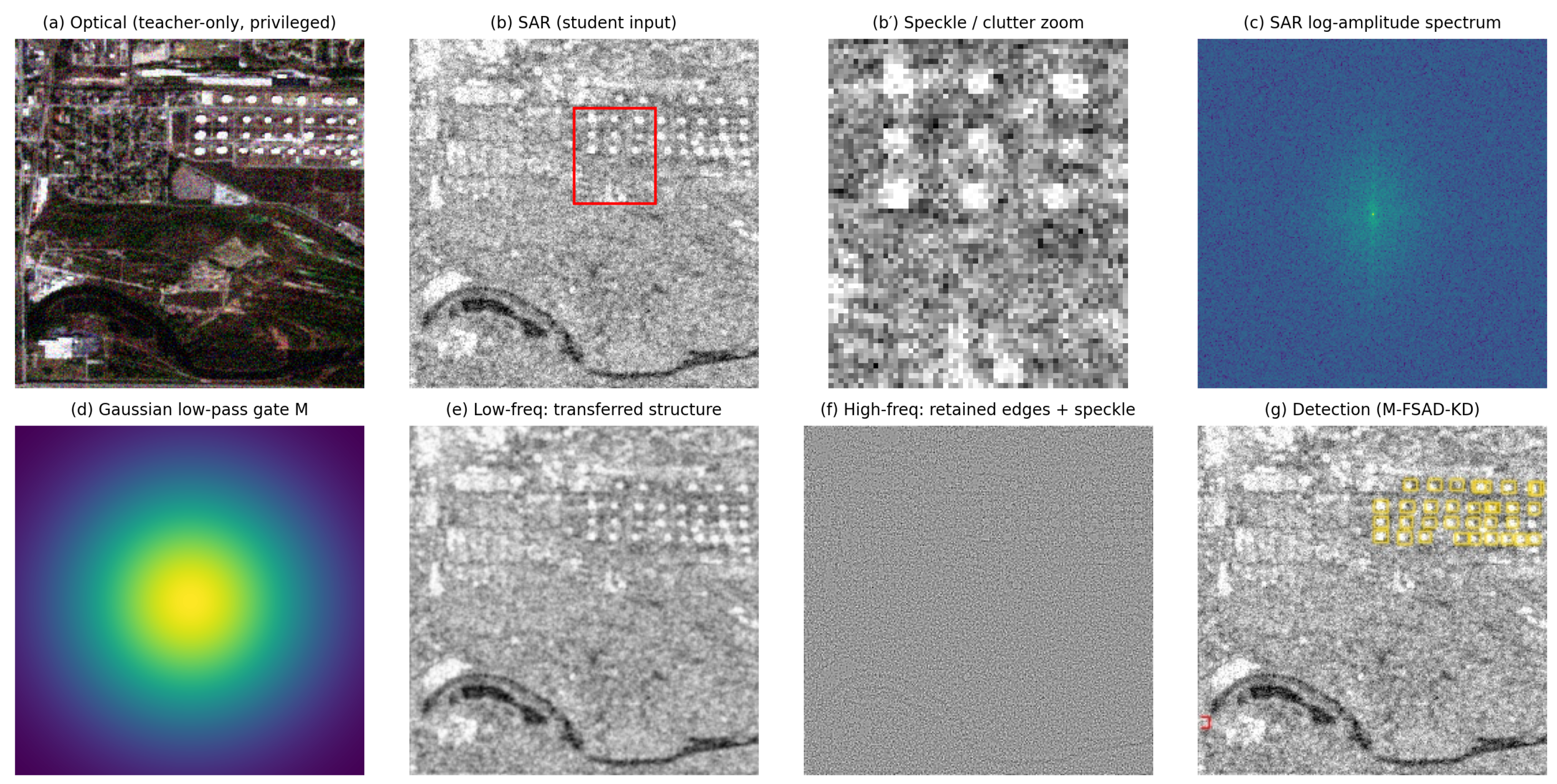
To make the frequency-decoupling principle concrete, Figure 2 walks through it on a representative OGSOD-1.0 optical–SAR (synthetic aperture radar) scene. The optical image Figure 2a, available only to the teacher, provides a clean structural reference; the SAR image Figure 2b, the sole student input, carries the same structure contaminated by multiplicative speckle (magnified in the inset). The 2D Fourier log-amplitude spectrum of the SAR image Figure 2c exposes the energy layout that motivates the mask: structural content concentrates near the low-frequency center, whereas speckle spreads broadly across the high-frequency plane. Applying the Gaussian low-pass gate ${\mathbf{M}}_{\mathrm{freq}}$ Figure 2d and inverting the retained band yields the low-frequency component Figure 2e—the structure that ${\mathcal{L}}_{\mathrm{freq}}$ transfers from teacher to student—while the complementary high-frequency component Figure 2f, which mixes target edges with speckle, carries no alignment gradient and is left to the student, so that the target-edge information needed for small-object localization is preserved rather than suppressed. The resulting M-FSAD-KD detections are shown in Figure 2g.

3.4. Joint Spatial–Channel Attention Distillation (JSCAD)

Even after frequency decoupling, the residual low-frequency content still contains background structure (sea surface, urban footprint) that is irrelevant to target localization. To steer the alignment gradient toward target-bearing regions, we construct a 3D joint mask ${\mathbf{M}}_{\mathrm{joint}}\in {\mathbb{R}}^{C\times H\times W}$ from the teacher’s feature statistics. We compute a spatial saliency map and a channel discriminability vector,

$${\mathbf{A}}_{\mathrm{sp}}(i,j)={\displaystyle \frac{1}{C}}\sum _c|{\mathbf{F}}_T^{\left(c\right)}(i,j)|,{\mathbf{A}}_{\mathrm{ch}}\left(c\right)={\displaystyle \frac{1}{HW}}\sum _{i,j}\left|{\mathbf{F}}_T^{\left(c\right)}(i,j)\right|,$$

(6)

followed by min-max normalization and broadcast outer product:

$${\mathbf{M}}_{\mathrm{joint}}=\mathrm{Norm}\left({\mathbf{A}}_{\mathrm{sp}}\right)\otimes \mathrm{Norm}\left({\mathbf{A}}_{\mathrm{ch}}\right).$$

(7)

The JSCAD loss is the mask-modulated squared error:

$${\mathcal{L}}_{\mathrm{jscad}}={\displaystyle \frac{1}{CHW}}\sum _{c,i,j}{\mathbf{M}}_{\mathrm{joint}}(c,i,j){\left({\mathbf{F}}_S^{\left(c\right)}(i,j)-{\mathbf{F}}_T^{\left(c\right)}(i,j)\right)}^2.$$

(8)

The mask is computed from the teacher and is, therefore, static within each forward pass; it does not introduce extra learnable parameters.

3.5. Response-Level Calibration (KD)

At the head end, we apply Hinton’s logit distillation [11] with temperature $\tau$. Following the YOLOv11 decoupled-head convention, classification logits $z_T,z_S\in {\mathbb{R}}^{B\times n_c\times A}$ are extracted from the teacher and student detectors, where $n_c$ denotes the number of object classes and A the total number of anchor locations across feature pyramid levels; the softmax is taken along the class dimension:

$$p_T={\mathrm{Softmax}}_{n_c}(z_T/\tau ),p_S={\mathrm{Softmax}}_{n_c}(z_S/\tau ),$$

(9)

$${\mathcal{L}}_{\mathrm{kd}}={\tau }^2·\mathrm{KL}(p_T\parallel p_S)={\tau }^2\sum _k{p}_T^{\left(k\right)}log{\displaystyle \frac{p_T^{\left(k\right)}}{p_S^{\left(k\right)}}}.$$

(10)

We set $\tau =10.0$. The KD term provides a final calibration of the classification decision boundary on top of the feature manifold purified by Bk, Freq, and JSCAD.

3.6. Full Objective and Dimensional-Homogenization Calibration

The total optimization objective is

$${\mathcal{L}}_{\mathrm{total}}={\mathcal{L}}_{\det }+{\lambda }_{\mathrm{bk}}{\mathcal{L}}_{\mathrm{bk}}+{\lambda }_{\mathrm{freq}}{\mathcal{L}}_{\mathrm{freq}}+{\lambda }_{\mathrm{jscad}}{\mathcal{L}}_{\mathrm{jscad}}+{\lambda }_{\mathrm{kd}}{\mathcal{L}}_{\mathrm{kd}},$$

(11)

where ${\mathcal{L}}_{\det }$ aggregates box regression, objectness, and classification. The four distillation losses operate at different feature scales and use different functional forms, so their raw magnitudes differ by orders of magnitude. We address this with a two-step calibration. First, the backward gradient norm of each loss term is tracked over the first epoch and the weights are set so that the four terms contribute comparable gradient magnitudes; this initial-gradient-magnitude calibration yields the ratio

$${\lambda }_{\mathrm{bk}}:{\lambda }_{\mathrm{freq}}:{\lambda }_{\mathrm{jscad}}:{\lambda }_{\mathrm{kd}}=100.0:45.0:10.0:0.12,$$

(12)

at which the total distillation loss begins at approximately $0.88$ times the detection loss. Second, the loss-weight sensitivity analysis in Section 4 identifies ${\lambda }_{\mathrm{freq}}=80.0$ as the empirical optimum on OGSOD-1.0. We, therefore, adopt

$${\lambda }_{\mathrm{bk}}:{\lambda }_{\mathrm{freq}}:{\lambda }_{\mathrm{jscad}}:{\lambda }_{\mathrm{kd}}=100.0:80.0:10.0:0.12$$

(13)

as the final configuration throughout the comparison, ablation, and deployment experiments. Under this configuration, the Freq and JSCAD terms operate at comparable gradient magnitudes, so that frequency decoupling and joint spatial–channel focusing remain co-active throughout training.

3.7. Relationship to Prior Multi-Modal Detectors

The relationship between M-FSAD-KD and existing multi-modal SAR–optical detectors—including our concurrent work MAIENet [6]—is one of complementary roles. Multi-modal detectors construct a joint SAR–optical representation under the assumption of complete modality availability at inference; M-FSAD-KD transfers such a representation to a unimodal SAR student that operates under modality absence at inference. A strong multi-modal teacher is, therefore, a pre-condition for effective distillation, while the methodological contributions of this paper—the speckle-fitting-trap diagnosis, the frequency-decoupled gating, the JSCAD mask, and the dimensional-homogenization calibration—are empirically consistent across the two teacher architectures we evaluate (Section 4.4.2). We adopt MAIENet as the primary teacher because it offers high accuracy at a controlled parameter budget on the same benchmark used for student evaluation; the cross-architecture experiment with the dual-stream DEYOLO teacher in Section 4.4.2 confirms that the framework transfers across teacher architecture families without per-teacher re-engineering.

3.8. Theoretical Analysis: Why Spatial-Distance Distillation Fails on SAR

This subsection provides a formal characterization of the speckle-fitting trap and supplies a theoretical basis for the empirical bandwidth ${\sigma }_f=min(H,W)/4$ adopted in the frequency-decoupled distillation of Section 3.

3.8.1. Additive Feature Decomposition and Spectral Assumptions

The student-side neck feature ${\mathbf{F}}_S\in {\mathbb{R}}^{C\times H\times W}$ admits the additive decomposition

$${\mathbf{F}}_S={\mathbf{S}}_S+\mathbf{N},$$

(14)

where ${\mathbf{S}}_S$ encodes the target scattering topology and $\mathbf{N}$ encodes the multiplicative SAR speckle component projected into the feature space. We stress that the additive form of Equation (14) is a first-order (small-fluctuation) approximation in feature space, not an image-domain identity: SAR speckle is multiplicative in the image, $\mathbf{x}=\mathbf{s}(1+\epsilon )$ with a zero-mean fluctuation $\epsilon$ of variance $\approx 1/L$ for an L-look image, but a first-order Taylor expansion of a neck feature map $\mathbf{F}(·)$ about the clean signal gives $\mathbf{F}\left(\mathbf{x}\right)\approx \mathbf{F}\left(\mathbf{s}\right)+{\mathbf{J}}_{\mathbf{F}}\left(\mathbf{s}\right)\left(\mathbf{s}\epsilon \right)={\mathbf{S}}_S+\mathbf{N}$, an additive feature perturbation $\mathbf{N}$ whose covariance is set by the network Jacobian and the speckle variance. The approximation is valid when the higher-order term $O\left({\epsilon }^2\right)$ is small—moderate-to-high look number, and after the variance-reducing batch-normalization and pooling layers that precede the neck; we no longer treat it as exact. Because fully developed speckle is spatially white and the early convolutional Jacobian is approximately shift-invariant, $\mathbf{N}$ remains approximately wide-band in feature space, which is precisely the property (Assumption 2) that the frequency-decoupled loss exploits. Because the teacher receives the optical stream in parallel, optical texture suppresses the speckle component in the teacher’s latent activation; to first order we, therefore, approximate the teacher feature by its structural component ${\mathbf{F}}_T\approx {\mathbf{S}}_T$, with the residual teacher-side speckle assumed to be of lower magnitude than $\mathbf{N}$ in the student.

Let $\mathcal{F}\{·\}$ denote the 2D Fourier transform. Two physically motivated assumptions follow from the SAR imaging literature.

Assumption 1

(Signal band-limitedness). The structural content of bridges, harbors and oil tanks is approximately band-limited to a low-frequency region ${\mathcal{B}}_S=\{(u,v):d(u,v)<{\rho }_S\}$:

$${\int }_{(u,v)\notin {\mathcal{B}}_S}{\left|\mathcal{F}\left\{\mathbf{S}\right\}(u,v)\right|}^2\mathrm{d}u\mathrm{d}v\le {\eta }_S\int {\left|\mathcal{F}\left\{\mathbf{S}\right\}\right|}^2\mathrm{d}u\mathrm{d}v,$$

(15)

with ${\eta }_S\ll 1$ a band-leakage upper bound.

Assumption 2

(Speckle wide-band uniformity). For any frequency subset $\mathcal{A}$,

$${\displaystyle \frac{{\int }_{\mathcal{A}}{\left|\mathcal{F}\left\{\mathbf{N}\right\}\right|}^2\mathrm{d}u\mathrm{d}v}{{\int \left|\mathcal{F}\left\{\mathbf{N}\right\}\right|}^2\mathrm{d}u\mathrm{d}v}}\approx {\displaystyle \frac{\left|\mathcal{A}\right|}{HW}},$$

(16)

i.e., speckle power is approximately uniform across the frequency plane. This assumption is consistent with the Goodman SAR speckle model summarized in [1].

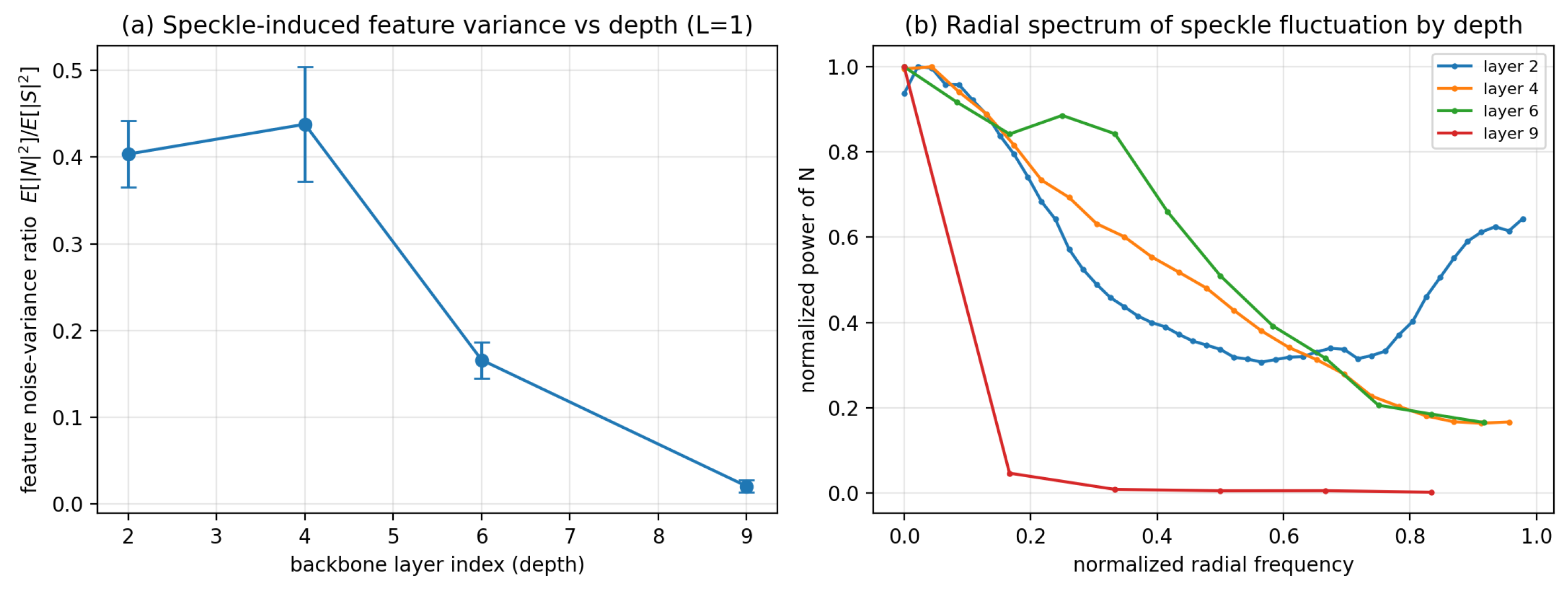
These assumptions, together with the first-order additive approximation, are supported empirically on the non-distilled SAR-only student. Using a Monte-Carlo estimate over 16 independent speckle realizations of 50 OGSOD-1.0 SAR images, we decompose each backbone feature into a structural component $\mathbf{S}\approx \mathbb{E}\left[\mathbf{F}\right]$ and a speckle fluctuation $\mathbf{N}=\mathbf{F}-\mathbf{S}$; the non-distilled student is used deliberately, so as to isolate the intrinsic forward propagation of speckle rather than any distillation effect. Figure 3 exhibits two properties. First, the feature noise-variance ratio ${\mathbb{E}[\parallel \mathbf{N}\parallel }^2{]/\mathbb{E}[\parallel \mathbf{S}\parallel }^2]$ decays sharply with depth, from ≈0.44 at the shallow backbone stages to ≈0.02 at the deepest stage, so the higher-order term $O\left({\epsilon }^2\right)$ is negligible at the deep stages where the distillation alignment operates—the regime in which the first-order expansion is accurate. Second, the radial power spectrum of $\mathbf{N}$ is wide-band at the shallow-to-mid stages (≈60–$63\%$ of its power lies beyond normalized radial frequency $0.2$, consistent with Assumption 2) and is progressively low-passed by the hierarchical downsampling to a near-DC residual (≈2%) only at the deepest stage. Both panels are essentially unchanged between $L=1$ and $L=4$, indicating the pattern is robust to the speckle level.

3.8.2. Gradient Pollution Under Spatial-Distance Distillation

Consider the conventional spatial MSE distillation loss

$${\mathcal{L}}_{\mathrm{MSE}}=\parallel {\mathbf{F}}_S-{\mathbf{F}}_T{\parallel }_2^2={\parallel {\mathbf{S}}_S+\mathbf{N}-{\mathbf{S}}_T\parallel }_2^2.$$

(17)

Differentiating with respect to ${\mathbf{F}}_S$ and grouping the signal and noise terms yields

$${\nabla }_{{\mathbf{F}}_S}{\mathcal{L}}_{\mathrm{MSE}}=\underset{{\mathbf{g}}_{\mathrm{sig}}}{\underbrace{2({\mathbf{S}}_S-{\mathbf{S}}_T)}}+\underset{{\mathbf{g}}_{\mathrm{noise}}}{\underbrace{2\mathbf{N}}}.$$

(18)

By Parseval’s identity, the energy ratio between the two gradient components satisfies

$${\displaystyle \frac{\parallel {\mathbf{g}}_{\mathrm{noise}}{\parallel }_2^2}{\parallel {\mathbf{g}}_{\mathrm{sig}}{\parallel }_2^2}}={\displaystyle \frac{{\parallel \mathcal{F}\left\{\mathbf{N}\right\}\parallel }_2^2}{\parallel \mathcal{F}\{{\mathbf{S}}_S-{\mathbf{S}}_T\}{\parallel }_2^2}}.$$

(19)

Empirically, the normalized speckle variance of a single-look SAR image is close to unity, whereas the post-Bk signal mismatch $\parallel {\mathbf{S}}_S-{\mathbf{S}}_T\parallel$ is materially smaller than $\parallel \mathbf{N}\parallel$ because Bk has already aligned the student and teacher on the structural manifold. The ratio in Equation (8) is, therefore, substantially larger than one, and the noise-fitting gradient ${\mathbf{g}}_{\mathrm{noise}}$ overwhelms the signal-fitting gradient ${\mathbf{g}}_{\mathrm{sig}}$ in determining the optimizer’s update direction. This constitutes the gradient-domain formulation of the speckle-fitting trap.

Remark on the severity gradient across spatial-distance methods. The decomposition in Equation (18) describes a generic spatial MSE loss; however, the magnitude of the trap depends on whether the loss further amplifies the noise channel through normalization or attention re-weighting. A plain per-pixel MSE (e.g., FitNet) spreads ${\mathbf{g}}_{\mathrm{noise}}$ uniformly over the spatial plane: the speckle component contributes to the loss but does not preferentially steer the gradient toward a particular spatial mode, so the student suffers a noise-fitting overhead that caps its gain rather than a catastrophic misallocation. In contrast, channel-wise softmax KL (e.g., CWD) re-normalizes the per-channel spatial distribution before computing the divergence, which mathematically promotes the broadband speckle to a dominant pattern within each channel and concentrates gradient mass on the speckle modes; masked-reconstruction variants (e.g., MGD) sit between these two regimes. Frequency decoupling removes the speckle band at the source and is, therefore, independent of which spatial re-normalization the downstream loss uses, restoring the trap-free optimization direction across all of these baselines.

3.8.3. Gradient Purification by Frequency-Decoupled Distillation

Replacing the spatial MSE with the masked frequency-domain loss in Section 3, namely

$${\mathcal{L}}_{\mathrm{freq}}=\sum _{u,v}{\mathbf{M}}_{\mathrm{freq}}(u,v){\left|\mathcal{F}\{{\mathbf{F}}_S-{\mathbf{F}}_T\}(u,v)\right|}^2,$$

(20)

its gradient decomposes by linearity as

$$\nabla {\mathcal{L}}_{\mathrm{freq}}={\mathcal{F}}^{-1}\left\{2{\mathbf{M}}_{\mathrm{freq}}\mathcal{F}\{{\mathbf{S}}_S-{\mathbf{S}}_T\}\right\}+{\mathcal{F}}^{-1}\left\{2{\mathbf{M}}_{\mathrm{freq}}\mathcal{F}\left\{\mathbf{N}\right\}\right\}.$$

(21)

Substituting Assumption 2 into the second term, the residual noise-gradient energy after frequency gating is

$$\parallel {\mathbf{M}}_{\mathrm{freq}}{\mathcal{F}\left\{\mathbf{N}\right\}\parallel }_2^2\approx {\displaystyle \frac{{\parallel \mathcal{F}\left\{\mathbf{N}\right\}\parallel }_2^2}{HW}}\sum _{u,v}{\mathbf{M}}_{\mathrm{freq}}{(u,v)}^2.$$

(22)

For a 2D Gaussian mask of bandwidth ${\sigma }_f$, the squared mask integral satisfies $\sum {\mathbf{M}}_{\mathrm{freq}}^2\approx \pi {\sigma }_f^2$, while the full spectral plane has area $HW$. The residual noise gradient is, therefore, attenuated by approximately the factor $\pi {\sigma }_f^2/\left(HW\right)$.

Proposition 1

(Noise-gradient suppression rate). With the empirical choice ${\sigma }_f=min(H,W)/4$, the noise-fitting gradient energy is reduced to approximately $\pi /16\approx 19.6\%$ of its un-gated value. That is, frequency gating suppresses roughly $80\%$ of the speckle-induced gradient pollution.

Proposition 2

(Signal preservation rate). Under Assumption 1, choosing ${\sigma }_f\ge {\rho }_S/2$ guarantees that the signal-gradient energy is preserved at a rate of at least $1-{\eta }_S$. The effective band edge ${\rho }_S$ depends on target geometry and image resolution; for OGSOD-1.0 targets we empirically estimate ${\rho }_S\lesssim min(H,W)/6$ from the teacher–student feature spectra (cf. Section 4), so ${\sigma }_f=min(H,W)/4$ lies safely above this lower bound and preserves more than $95\%$ of the signal energy in practice.

3.8.4. Scope of the Trap: When Spatial-Distance Losses Do and Do Not Suffer

The gradient pollution analyzed above corresponds to a worst-case bound. In practice, the severity of the trap depends on how each loss re-weights or normalizes the spatial residual before back-propagation. Uniform spatial MSE (e.g. FitNet [18]) distributes the noise gradient evenly across spatial positions, so any single speckle pixel contributes only $O(1/(HW\left)\right)$ to the gradient norm: the trap is present but attenuated, and the student typically achieves a small positive gain over the non-distilled baseline (cf. Section 4). The trap becomes severe when the loss concentrates or amplifies structure-correlated noise: in CWD [23], a per-channel softmax renormalizes the spatial distribution within each channel and forces the student to reproduce the broadband speckle statistics; in mask-based variants such as the focal mask of FGD [19] or the random spatial mask of MGD [20], partial overlap between the mask support and the speckle support can re-concentrate gradient mass on noise pixels. The empirical pattern reported in Section 4—CWD degrades below the baseline, MGD remains at the baseline, and FitNet exhibits a small positive gain—is consistent with this gradient-distribution argument.

3.8.5. Optimal Bandwidth Range

Combining the two propositions, the optimal cut-off bandwidth ${\sigma }_f^{\star }$ is the trade-off between two opposing requirements: a lower bound ${\sigma }_f\ge {\rho }_S/2\approx min(H,W)/12$ that preserves signal energy, and an upper bound ${\sigma }_f\le min(H,W)/2$ beyond which the Gaussian mask degenerates into an approximate identity and the frequency-gating mechanism vanishes. The empirical choice ${\sigma }_f=min(H,W)/4$ sits in the middle of this admissible interval, corresponding to the operating point of “signal almost fully preserved, noise heavily suppressed”. The non-monotonic behavior reported in Section 4 (Group I of the weight-sensitivity sweep)—accuracy rising from ${\lambda }_{\mathrm{freq}}=45$ to 80 and then declining at ${\lambda }_{\mathrm{freq}}=120$—is consistent with this prediction: stronger ${\lambda }_{\mathrm{freq}}$ effectively narrows the operating bandwidth, first further suppressing noise (Proposition 1) and eventually violating the signal-preservation lower bound (Proposition 2).

3.8.6. Generality to Other Modality Pairs

Both assumptions used above are not specific to SAR. Any modality pair that satisfies a low-frequency band-limited signal hypothesis together with a wide-band noise component—representative examples include RGB–infrared, RGB–depth, and visible–hyperspectral—falls within the same theoretical framework. The frequency-decoupled distillation should, therefore, extend to such modality pairs without methodological modification, as long as the bandwidth ${\sigma }_f$ is calibrated to the new signal support. We treat this generalization as a direction for future empirical validation.

4. Experiments and Results

4.1. Dataset

We evaluate on OGSOD-1.0 [5], the largest publicly available rigorously co-registered SAR–optical detection benchmark. The dataset contains 14,665 paired training samples and 3666 paired test samples, covering three target categories: bridges (31,922 instances), harbors (4109 instances), and oil tanks (12,558 instances). The SAR images originate from the Chinese GaoFen-3 satellite (C-band, VV/VH polarizations, 3 m ground sampling distance); the corresponding optical images are sourced from Google Earth at 10 m ground sampling distance. To minimize temporal decorrelation, optical imagery was selected within one month of the SAR acquisition date. Both modalities are resampled to a common spatial grid and cropped to $256\times 256$ pixels. Approximately 90% of annotated instances cover less than $35\times 35$ pixels, and the oil-tank category in particular consists almost exclusively of small targets (99.9% smaller than $32\times 32$).

4.2. Asymmetric Cross-Modal Protocol and Experimental Environment

We design an asymmetric cross-modal protocol that strictly separates the training and inference modality budgets. During training, the teacher network has access to both SAR and optical streams and is queried by the student through the M-FSAD-KD framework. During inference, the student takes only the SAR stream as input; the optical stream and all distillation components are completely absent. This protocol simulates the on-board failure of the optical sensor or the disruption of the synchronized downlink under adversarial conditions.

Teacher. We adopt MAIENet [6] as the primary multi-modal teacher (34.0 M parameters, 27.6 GFLOPs, ${\mathrm{mAP}}_{50}=90.8\%$ on OGSOD-1.0). The choice of MAIENet is motivated by its high accuracy at a controlled parameter budget on the same benchmark used for student evaluation; however, the distillation components proposed in this paper are not tied to MAIENet’s specific architecture, as confirmed on the two teacher architectures tested in Section 4.4.2. This claim is empirically verified by an additional cross-architecture experiment with a dual-stream DEYOLO [13] teacher, reported in Section 4.

Student. The student is a lightweight YOLOv11n* [27], in which the original PSA module is removed and the second backbone layer is replaced with a multi-direction focus operator. The student has 2.39 M parameters and 1.29 GFLOPs at $256\times 256$ input resolution. To evaluate the framework at a higher capacity, we additionally distill a YOLOv11m* student (19.98 M parameters, 15.32 GFLOPs).

Training. We use stochastic gradient descent with an initial learning rate of $0.01$, momentum $0.937$, and weight decay $5\times {10}^{-4}$, with a batch size of 64. Comparative experiments use 100 epochs to evaluate convergence-rate efficiency under a controlled budget; deployment-level experiments use 400 epochs for full convergence. Distillation weights are set to ${\lambda }_{\mathrm{bk}}:{\lambda }_{\mathrm{freq}}:{\lambda }_{\mathrm{jscad}}:{\lambda }_{\mathrm{kd}}=100.0:80.0:10.0:0.12$ unless otherwise stated, following the calibration and sensitivity analysis of Section 3. All experiments were run on NVIDIA RTX 3090 GPUs. To keep the comparison fair, within any single comparison table every method—the non-distilled baseline, all distillation baselines, and M-FSAD-KD—is trained under an identical budget, hardware, student backbone, and teacher; no method is given more epochs than another. The 100- and 400-epoch settings, therefore, never mix within one comparison:

Table 1. Performance evaluation of unimodal baseline models with different capacities (400 epochs). Abbreviations: AP, average precision (Bri., bridge; Har., harbour; Tan., oil tank); P, precision; R, recall; mAP, mean average precision; Params, number of parameters; GFLOPs, giga floating-point operations.

Method	Type	${\mathbf{AP}}_{\mathbf{Bri}.}$	${\mathbf{AP}}_{\mathbf{Har}.}$	${\mathbf{AP}}_{\mathbf{Tan}.}$	P (%)	R (%)	${\mathbf{mAP}}_{50}$	${\mathbf{mAP}}_{50:95}$	Params (M)	GFLOPs (G)
MAIENet (Teacher)	Multi-Modal	93.8	99.4	79.0	91.2	86.1	90.8	61.0	34.00	27.60
YOLOv11m	Single-Modal	81.6	99.4	47.5	82.1	71.3	76.2	50.1	20.23	10.80
YOLOv11m*	Single-Modal	76.4	98.7	47.0	81.4	69.3	74.0	47.5	19.98	15.32
YOLOv11s	Single-Modal	68.7	97.7	34.1	74.3	62.8	66.9	42.1	9.41	3.40
YOLOv11s*	Single-Modal	66.3	97.1	31.1	73.8	61.3	64.8	40.8	8.66	4.48
YOLOv11n	Single-Modal	56.9	94.2	18.7	62.5	55.5	56.6	34.6	2.58	1.03
YOLOv11n*	Single-Modal	57.4	94.0	21.8	65.8	55.3	57.7	35.3	2.39	1.29

uses the 400-epoch setting for the student-selection screen, Table 2 and Table 3 use the 100-epoch setting for the method-vs-method comparison, and Table 9 uses the 400-epoch setting for the deployment upper bound, where the baseline and M-FSAD-KD are likewise both trained for 400 epochs.

Evaluation. We follow the COCO protocol [28], reporting ${\mathrm{mAP}}_{50}$, ${\mathrm{mAP}}_{50:95}$, and per-class AP.

Table 2. Cross-modal distillation comparison on OGSOD-1.0 (100 epochs, student YOLOv11n*, teacher MAIENet, all rows trained on the same hardware platform under the canonical weight configuration ${\lambda }_{\mathrm{bk}}:{\lambda }_{\mathrm{freq}}:{\lambda }_{\mathrm{jscad}}:{\lambda }_{\mathrm{kd}}=100:80:10:0.12$). Values are single representative runs, except the SDD, LSKD and LDRLD rows, which are 3-seed means; multi-seed mean±std for the non-distilled baseline, CWD, KD, and M-FSAD-KD are reported in Table 3 (the M-FSAD-KD entry here is the best of the runs, mean $47.9\pm 0.9$). Best results in each column are in bold.

Method	Backbone	Type	${\mathbf{AP}}_{\mathbf{Bri}.}$	${\mathbf{AP}}_{\mathbf{Har}.}$	${\mathbf{AP}}_{\mathbf{Tan}.}$	${\mathbf{mAP}}_{50}$	${\mathbf{mAP}}_{50:95}$
Baseline (Student)	YOLOv11n*	Single-Modal	44.1	75.3	11.4	43.6	22.9
CWD [23]	YOLOv11n*	Channel	43.7	73.2	9.85	42.2	21.8
MGD [20]	YOLOv11n*	Masked	44.6	74.3	11.1	43.3	23.4
FitNet [18]	YOLOv11n*	Feature	45.6	77.1	12.1	44.9	24.0
FGD [19]	YOLOv11n*	Focal+Global	45.4	79.1	11.5	45.3	24.7
DKD [22]	YOLOv11n*	Decoupled	47.5	80.1	13.2	46.9	24.3
LD [21]	YOLOv11n*	Localization	46.7	82.4	12.0	47.0	26.0
KD [17]	YOLOv11n*	Logits	48.2	84.1	13.1	48.4	26.3
SDD [29]	YOLOv11n*	Scale-decoup.	44.3	75.6	11.9	43.9	23.1
LSKD [30]	YOLOv11n*	Logit-std.	45.3	74.8	12.2	44.1	22.9
LDRLD [31]	YOLOv11n*	Logit-rel.	47.9	84.4	11.1	47.8	25.8
M-FSAD (Ours, no head KD)	YOLOv11n*	Feature	47.7	83.3	12.3	47.8	26.5
M-FSAD-KD (Ours)	YOLOv11n*	Full-Link	48.6	86.5	14.0	49.7	28.3

Table 2. Cross-modal distillation comparison on OGSOD-1.0 (100 epochs, student YOLOv11n*, teacher MAIENet, all rows trained on the same hardware platform under the canonical weight configuration ${\lambda }_{\mathrm{bk}}:{\lambda }_{\mathrm{freq}}:{\lambda }_{\mathrm{jscad}}:{\lambda }_{\mathrm{kd}}=100:80:10:0.12$). Values are single representative runs, except the SDD, LSKD and LDRLD rows, which are 3-seed means; multi-seed mean±std for the non-distilled baseline, CWD, KD, and M-FSAD-KD are reported in Table 3 (the M-FSAD-KD entry here is the best of the runs, mean $47.9\pm 0.9$). Best results in each column are in bold.

Method	Backbone	Type	${\mathbf{AP}}_{\mathbf{Bri}.}$	${\mathbf{AP}}_{\mathbf{Har}.}$	${\mathbf{AP}}_{\mathbf{Tan}.}$	${\mathbf{mAP}}_{50}$	${\mathbf{mAP}}_{50:95}$
Baseline (Student)	YOLOv11n*	Single-Modal	44.1	75.3	11.4	43.6	22.9
CWD [23]	YOLOv11n*	Channel	43.7	73.2	9.85	42.2	21.8
MGD [20]	YOLOv11n*	Masked	44.6	74.3	11.1	43.3	23.4
FitNet [18]	YOLOv11n*	Feature	45.6	77.1	12.1	44.9	24.0
FGD [19]	YOLOv11n*	Focal+Global	45.4	79.1	11.5	45.3	24.7
DKD [22]	YOLOv11n*	Decoupled	47.5	80.1	13.2	46.9	24.3
LD [21]	YOLOv11n*	Localization	46.7	82.4	12.0	47.0	26.0
KD [17]	YOLOv11n*	Logits	48.2	84.1	13.1	48.4	26.3
SDD [29]	YOLOv11n*	Scale-decoup.	44.3	75.6	11.9	43.9	23.1
LSKD [30]	YOLOv11n*	Logit-std.	45.3	74.8	12.2	44.1	22.9
LDRLD [31]	YOLOv11n*	Logit-rel.	47.9	84.4	11.1	47.8	25.8
M-FSAD (Ours, no head KD)	YOLOv11n*	Feature	47.7	83.3	12.3	47.8	26.5
M-FSAD-KD (Ours)	YOLOv11n*	Full-Link	48.6	86.5	14.0	49.7	28.3

Table 3. Multi-seed, capacity-resolved comparison against the non-distilled baseline, strong response-level KD, and three recent logit-level methods (SDD [29], LSKD [30], LDRLD [31]) on OGSOD-1.0 (100 epochs; mean ± std over 3–5 seeds, same training pipeline for every row). M-FSAD-KD is on par with KD at the 2.39 M capacity and, at 19.98 M, exceeds KD by $2.0$ points and the strongest recent logit method (LDRLD) by $1.7$ points. Best per block in bold.

Student	Method	${\mathbf{mAP}}_{50}$ (%)	${\mathbf{mAP}}_{50:95}$ (%)
YOLOv11n* (2.39 M)	Baseline (no distillation)	$43.3\pm 0.6$	$22.8\pm 0.2$
YOLOv11n* (2.39 M)	CWD	$41.8\pm 0.3$	$21.4\pm 0.3$
YOLOv11n* (2.39 M)	KD	$48.1\pm 0.4$	$25.9\pm 0.3$
YOLOv11n* (2.39 M)	SDD	$43.9\pm 0.9$	$23.1\pm 0.5$
YOLOv11n* (2.39 M)	LSKD	$44.1\pm 0.4$	$22.9\pm 0.1$
YOLOv11n* (2.39 M)	LDRLD	$47.8\pm 0.4$	$25.8\pm 0.1$
YOLOv11n* (2.39 M)	M-FSAD-KD (Ours)	$47.9\pm 0.9$	$25.9\pm 1.4$
YOLOv11m* (19.98 M)	Baseline (no distillation)	$57.7\pm 0.3$	$33.0\pm 0.4$
YOLOv11m* (19.98 M)	KD	$63.6\pm 0.5$	$38.7\pm 0.2$
YOLOv11m* (19.98 M)	SDD	$58.9\pm 0.5$	$33.7\pm 0.3$
YOLOv11m* (19.98 M)	LSKD	$60.8\pm 0.2$	$35.4\pm 0.1$
YOLOv11m* (19.98 M)	LDRLD	$63.9\pm 0.2$	$39.3\pm 0.1$
YOLOv11m* (19.98 M)	M-FSAD-KD (Ours)	$\mathbf{65}.\mathbf{6}\pm \mathbf{0}.\mathbf{3}$	$\mathbf{41}.\mathbf{4}\pm \mathbf{0}.\mathbf{1}$

Table 3. Multi-seed, capacity-resolved comparison against the non-distilled baseline, strong response-level KD, and three recent logit-level methods (SDD [29], LSKD [30], LDRLD [31]) on OGSOD-1.0 (100 epochs; mean ± std over 3–5 seeds, same training pipeline for every row). M-FSAD-KD is on par with KD at the 2.39 M capacity and, at 19.98 M, exceeds KD by $2.0$ points and the strongest recent logit method (LDRLD) by $1.7$ points. Best per block in bold.

Student	Method	${\mathbf{mAP}}_{50}$ (%)	${\mathbf{mAP}}_{50:95}$ (%)
YOLOv11n* (2.39 M)	Baseline (no distillation)	$43.3\pm 0.6$	$22.8\pm 0.2$
YOLOv11n* (2.39 M)	CWD	$41.8\pm 0.3$	$21.4\pm 0.3$
YOLOv11n* (2.39 M)	KD	$48.1\pm 0.4$	$25.9\pm 0.3$
YOLOv11n* (2.39 M)	SDD	$43.9\pm 0.9$	$23.1\pm 0.5$
YOLOv11n* (2.39 M)	LSKD	$44.1\pm 0.4$	$22.9\pm 0.1$
YOLOv11n* (2.39 M)	LDRLD	$47.8\pm 0.4$	$25.8\pm 0.1$
YOLOv11n* (2.39 M)	M-FSAD-KD (Ours)	$47.9\pm 0.9$	$25.9\pm 1.4$
YOLOv11m* (19.98 M)	Baseline (no distillation)	$57.7\pm 0.3$	$33.0\pm 0.4$
YOLOv11m* (19.98 M)	KD	$63.6\pm 0.5$	$38.7\pm 0.2$
YOLOv11m* (19.98 M)	SDD	$58.9\pm 0.5$	$33.7\pm 0.3$
YOLOv11m* (19.98 M)	LSKD	$60.8\pm 0.2$	$35.4\pm 0.1$
YOLOv11m* (19.98 M)	LDRLD	$63.9\pm 0.2$	$39.3\pm 0.1$
YOLOv11m* (19.98 M)	M-FSAD-KD (Ours)	$\mathbf{65}.\mathbf{6}\pm \mathbf{0}.\mathbf{3}$	$\mathbf{41}.\mathbf{4}\pm \mathbf{0}.\mathbf{1}$

4.3. Student Network Architecture Selection

Before constructing the cross-modal distillation framework, we screen the YOLOv11 series at different capacity levels (Nano, Small, Medium) to select a student that balances edge-device computational limits with representation potential. Each candidate is trained for 400 epochs to ensure full convergence. We also introduce lightweight architectural improvements (denoted by an asterisk *) for each capacity level: the PSA module is removed and the second backbone layer is replaced with a more efficient multi-direction focus operator. The results are shown in Table 1.

Table 1 reveals a scale-inverted phenomenon. For Medium and Small capacity models, removing PSA leads to a slight performance drop (for example, YOLOv11m: 76.2% → 74.0%), indicating that the attention mechanism still helps maintain high-dimensional feature discriminability in larger networks. At the Nano capacity, however, the trend reverses. YOLOv11n*, despite being further pruned to 2.39 M parameters, lifts ${\mathrm{mAP}}_{50}$ by 1.1 absolute points and lifts the small-scale oil-tank AP from 18.7% to 21.8%. We attribute this to the fact that complex spatial-attention modules act as an optimization burden when the parameter space is extremely tight, whereas the streamlined architecture combined with the multi-direction focus operator extracts the basic geometric features of SAR targets more robustly. We, therefore, adopt YOLOv11n* as the single-modal student baseline. To fairly evaluate distillation efficiency under a controlled computational budget, all subsequent distillation comparison and ablation experiments are conducted under 100 epochs.

4.4. Comparison with Distillation Baselines

Table 2 compares M-FSAD-KD against ten distillation baselines under the same student backbone (YOLOv11n*) and the same teacher (MAIENet): channel-aligned distillation (CWD [23]), masked reconstruction (MGD [20]), generic feature alignment (FitNet [18]), focal-and-global feature alignment (FGD [19]), localization distillation (LD [21]), decoupled logits (DKD [22]), and standard response distillation (KD [17]). To ensure the comparison reflects the current state of the art, we additionally benchmark three of the most recent logit-level distillation methods: scale-decoupled distillation (SDD [29]), logit standardization (LSKD [30]), and local dense logit relations (LDRLD [31]).

Three patterns emerge from Table 2. First, CWD [23] is the only method that reduces the student’s ${\mathrm{mAP}}_{50}$ below the non-distilled baseline (42.2% vs. 43.6%, a degradation of 1.4 absolute points), with the impact concentrated on the smallest-target storage-tank class: CWD’s tank AP drops from the baseline’s 11.4% to 9.85% (a degradation of 1.55 absolute points). An independently trained run on a separate hardware platform reproduces this degradation in direction with an even more extreme tank AP of 0.10%, confirming that the magnitude varies across runs while the direction of degradation is robust. This empirically validates the speckle-fitting-trap hypothesis: the channel-wise softmax alignment of CWD distributes the optimization signal across the entire spatial extent of each channel, allowing broadband speckle energy to dominate the gradient and starve the smallest-target features. The remaining baselines either match the baseline within run-to-run variation (MGD [20] 43.3%) or yield positive gains of 1.3 to 4.8 absolute points on ${\mathrm{mAP}}_{50}$ (FitNet [18] 44.9%, FGD [19] 45.3%, DKD [22] 46.9%, LD [21] 47.0%, KD [17] 48.4%). The three most recent logit-level methods span only $43.9$–$47.8\%$ ${\mathrm{mAP}}_{50}$ (SDD $43.9\%$, LSKD $44.1\%$, LDRLD $47.8\%$) and none surpasses the classical response-level KD ($48.4\%$): SDD and LSKD sit within a point of the non-distilled baseline, while LDRLD merely matches KD. Even the latest refinements of logit distillation, therefore, plateau at the response-level ceiling on this cross-modal SAR task; none of them purifies the low-level feature manifold where the speckle-fitting trap originates.

Second, the proposed M-FSAD-KD attains the best ${\mathrm{mAP}}_{50}$ in the table (49.7% for the best run; $47.9\pm 0.9$ averaged over seeds, Table 3), ahead of every distillation baseline, including the strongest response-level KD and FGD by $4.4$ absolute points. We stress, however, that at this smallest (2.39 M) capacity the margin over KD is within run-to-run variation; the feature-distillation chain’s advantage over KD becomes clear-cut only at higher student capacity and under out-of-domain transfer, as quantified in Section 4.4.1. On the smallest-target storage-tank class, the full model raises AP well above CWD’s collapsed 9.85%, indicating that frequency-decoupled distillation shields small-target high-frequency features from the speckle pollution that sinks CWD.

Third, the head-end response distillation contributes a measurable lift on top of the feature-level chain: M-FSAD without the head-end KD attains 47.8%; adding the head-end KD raises it to the value reported for the full model, a lift that exceeds the observed run-to-run variation and indicates the soft-label calibration provides genuine value on top of the purified feature manifold rather than a spurious fluctuation.

4.4.1. Multi-Seed Variance, Capacity Scaling, and Feature Transferability

Because the single-run comparison in Table 2 cannot by itself establish that the feature-distillation chain is worth its added machinery over the strong response-level KD baseline, we re-train the non-distilled baseline, CWD, KD, the three most recent logit-level methods (SDD, LSKD, LDRLD), and M-FSAD-KD over multiple random seeds and, additionally, at a higher student capacity. The results (Table 3) reframe the contribution in a capacity-resolved way. At the 2.39 M capacity, M-FSAD-KD and KD are statistically indistinguishable ($47.9\pm 0.9$ vs. $48.1\pm 0.4$ ${\mathrm{mAP}}_{50}$, the sub-point difference lying within seed variance): a low-capacity student is largely saturated by the soft labels, consistent with the small individual-component effects noted in the ablation of Section 4. At the 19.98 M capacity, however, M-FSAD-KD exceeds KD by $2.0$ absolute points ($65.6$ vs. $63.6$, gain consistent across all three classes and both metrics) and the non-distilled baseline by $7.9$ points; it also surpasses the strongest of the three recent logit-level methods (LDRLD, $63.9$) by $1.7$ points, with SDD ($58.9$) and LSKD ($60.8$) trailing further behind. The advantage of the feature-level chain over response-only KD, therefore, emerges with the student’s representational capacity—a higher-capacity student can absorb privileged feature-level structure that soft labels alone cannot convey, whereas at the smallest capacity the two are on par.

The same conclusion holds under distribution shift. We freeze each OGSOD-distilled backbone-and-neck and train only a fresh detection head on the out-of-domain SSDD ship-detection benchmark—a frozen-feature (linear-probe) test of representation quality on a task with entirely different target classes. As

Table 4. Frozen-feature transfer (linear probe) to the out-of-domain SSDD ship-detection benchmark: each OGSOD-distilled backbone-and-neck is frozen and only a fresh detection head is trained (mean ± std over 3 seeds). Distilling from the multi-modal teacher yields far more transferable SAR features than no distillation or the trap-prone CWD, and M-FSAD-KD transfers best. Best in bold.

Frozen Source (Distilled on OGSOD-1.0)	SSDD ${\mathbf{mAP}}_{50}$ (%)	${\mathbf{mAP}}_{50:95}$ (%)
Non-distilled baseline	$73.3\pm 0.4$	$33.3\pm 0.1$
CWD (trap)	$74.4\pm 0.7$	$33.5\pm 0.4$
KD	$81.0\pm 0.5$	$37.9\pm 0.4$
M-FSAD-KD (Ours)	$\mathbf{82}.\mathbf{6}\pm \mathbf{0}.\mathbf{0}$	$\mathbf{40}.\mathbf{3}\pm \mathbf{0}.\mathbf{4}$

shows, distilling from the multi-modal teacher produces markedly more transferable SAR features than no distillation or the trap-prone CWD (81–83 vs. 73–74 ${\mathrm{mAP}}_{50}$), and M-FSAD-KD transfers best ($82.6$ vs. $81.0$ for response-level KD). The trap method (CWD) transfers no better than the non-distilled backbone, echoing the speckle-fitting-trap diagnosis. Together with the capacity result, this indicates that the feature-level chain yields a more useful, more transferable representation than response-only distillation once the representation must generalize to a new task or the student has the capacity to exploit it.

Frequency-Mask Ablation (Is It a Generic Low-Pass?)

A natural concern is whether the frequency gating is a specific low-pass mechanism or merely a generic low-pass regularizer. To answer it we isolate the frequency term on the Bk+Freq configuration (no JSCAD, no head-level KD), so the mask is the sole neck-alignment force, and sweep the mask shape (low-pass vs. high-pass vs. all-pass, i.e., ungated spectral MSE), the mask family (Gaussian vs. ideal hard cut-off), the cut-off $\sigma =min(H,W)/\{2,4,8\}$, and a spatial-domain Gaussian-blur “generic low-pass” control (

Table 5. Frequency-mask ablation on the Bk+Freq configuration (YOLOv11n*, 100 epochs, mean ± std over seeds). This reduced two-component (Bk+Freq) base is used to isolate the mask effect and, therefore, sits below the full four-granularity model of Table 3; the comparison of interest here is across mask variants, not against the full model. Accuracy is insensitive to the mask shape, family and cut-off, and to a spatial-blur generic-low-pass control, indicating the benefit is not tied to a specific low-pass profile.

Ablated Axis	Setting	${\mathbf{mAP}}_{50}$ (%)	${\mathbf{mAP}}_{50:95}$ (%)
Shape	Low-pass (default, $\sigma =min(H,W)/4$)	$46.4\pm 0.4$	$24.9\pm 0.4$
Shape	High-pass	$46.8\pm 0.6$	$25.4\pm 0.4$
Shape	All-pass (ungated spectral MSE)	$46.0\pm 0.6$	$24.3\pm 0.7$
Cut-off	$\sigma =min(H,W)/2$	$46.2\pm 1.1$	$24.4\pm 1.1$
Cut-off	$\sigma =min(H,W)/8$	$45.5\pm 1.4$	$24.3\pm 1.2$
Family	Ideal (hard cut-off)	$46.0\pm 0.8$	$24.7\pm 0.7$
Control	Spatial-blur “generic low-pass”	$47.1\pm 0.9$	$25.2\pm 0.1$

). Over repeated seeds, accuracy is statistically insensitive to the mask configuration: all variants fall within $46.0$–$47.1$ ${\mathrm{mAP}}_{50}$ with overlapping standard deviations, and the spatial-blur control is not inferior. We report this candidly. The frequency term’s benefit, therefore, does not stem from a particular spectral profile but from operating in the amplitude-spectrum domain, which—unlike CWD’s channel-wise softmax—does not renormalize each channel’s spatial distribution and hence does not let the broadband speckle mode dominate the alignment gradient (Section 3.8). The framework is robust to the mask choice, and we make no claim that low-pass gating is uniquely optimal.

4.4.2. Cross-Teacher-Architecture Validation

A central methodological claim of M-FSAD-KD is that the framework’s effectiveness depends on the privileged information conveyed by the multi-modal teacher, not on the teacher’s specific architectural choices. We verify this claim by replacing the MAIENet teacher with DEYOLO [13], a substantially different multi-modal detector. The two teachers contrast along three axes: backbone family (YOLO11 vs. YOLOv8 with BiFocus), stream topology (single-stream with deep modality-aware interaction vs. dual-stream with separate per-modality encoders), and thelocation of cross-modal fusion (deepest semantic stage vs. head-start DEA cross-attention). All other variables—student architecture (YOLOv11n*), training hyper-parameters, distillation weights, dataset, and seed—are held fixed; only the teacher is swapped. Results are reported in

Table 6. Cross-teacher-architecture validation on OGSOD-1.0 (100 epochs, student YOLOv11n*, all weights 100:80:10:0.12). Both teachers drive the same student well above the non-distilled baseline; the cross-architecture gap is only 1.1 absolute points on ${\mathrm{mAP}}_{50}$. Best result in each column is in bold.

Teacher	Teacher Architecture	${\mathbf{AP}}_{\mathbf{Bri}.}$	${\mathbf{AP}}_{\mathbf{Har}.}$	${\mathbf{AP}}_{\mathbf{Tan}.}$	${\mathbf{mAP}}_{50}$	${\mathbf{mAP}}_{50:95}$	${\Delta }_{\mathbf{base}}$
(none, baseline)	—	44.1	75.3	11.4	43.6	22.9	—
MAIENet [6]	Single-stream YOLO11m + deep MAI	48.6	86.5	14.0	49.7	28.3	+6.1
DEYOLO [13]	Dual-stream YOLOv8m + DEA cross-attn.	47.8	85.9	12.2	48.6	27.4	+5.0
DEYOLO (Bk disabled)	Dual-stream YOLOv8m + DEA cross-attn.	45.8	80.9	12.1	46.3	24.5	+2.7

.

The cross-architecture validation supports three observations. First, M-FSAD-KD with the DEYOLO teacher attains 48.6% ${\mathrm{mAP}}_{50}$, only 1.1 absolute points below the MAIENet-teacher result of 49.7%, despite the substantially different backbone family and dual-stream topology. The two teacher configurations jointly establish that M-FSAD-KD transfers across heterogeneous multi-modal teacher architectures with a cross-architecture gap of only 1.1 absolute points on ${\mathrm{mAP}}_{50}$. Second, both teachers lift the student well above the non-distilled baseline (gains of $+6.1$ and $+5.0$ absolute points, respectively), confirming that the framework’s effectiveness is not an artifact of MAIENet’s specific properties; the relatively larger gain with MAIENet is consistent with the closer architectural alignment between teacher and student (shared YOLO11 backbone family). Third, disabling the Bk shallow adaptation under the DEYOLO teacher drops the result from 48.6% to 46.3% ($-2.3$ absolute points) while still leaving the student 2.7 absolute points above the non-distilled baseline. This shows that the learnable $1\times 1$ channel adapter transfers backbone-level knowledge even when the teacher and student backbones use different operator families (DEYOLO’s C2f + BiFocus operators vs. the student’s C3k2 operators). The role of Bk—projecting student features into the teacher’s channel-aligned representation—is, therefore, operator-family-agnostic in practice, and the design choice of using a lightweight projection rather than relying on architectural compatibility is empirically supported.

Taken together, the cross-architecture results indicate that M-FSAD-KD transfers across the two representative teacher architecture families tested: a sufficiently strong multi-modal SAR–optical teacher of either single-stream or dual-stream topology can be paired with the same student under the same framework, without per-teacher re-engineering of the distillation loss; validation on a broader range of teacher architectures is left to future work.

4.4.3. Speckle-Fitting Trap: Frequency and Manifold Evidence

The empirical degradation of CWD reported above is unusual in the homogeneous-modality KD literature and, therefore, deserves direct frequency-domain evidence. This subsection provides four complementary diagnostics—teacher-student spectral comparison, method-wise spectral evolution, post-training residual band decomposition, and feature-manifold geometry—to establish the trap as a measurable physical phenomenon and to characterize how frequency-decoupled distillation counteracts it. All quantitative values reported here are extracted directly from the analysis pipeline executed on the OGSOD-1.0 validation set (200 images, P4 features, $16\times 16$ spatial resolution at input resolution $256\times 256$).

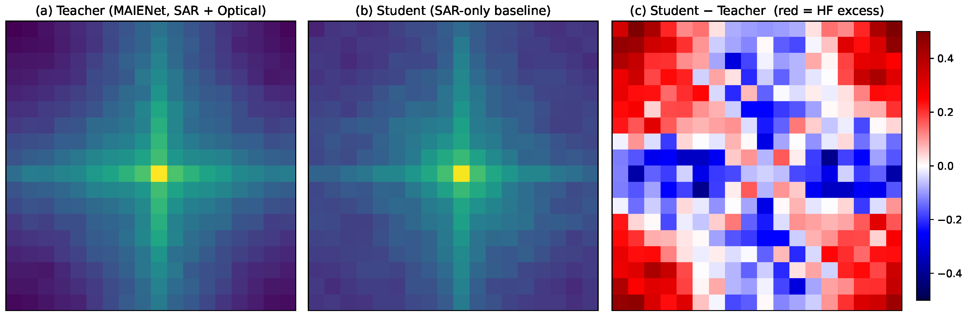
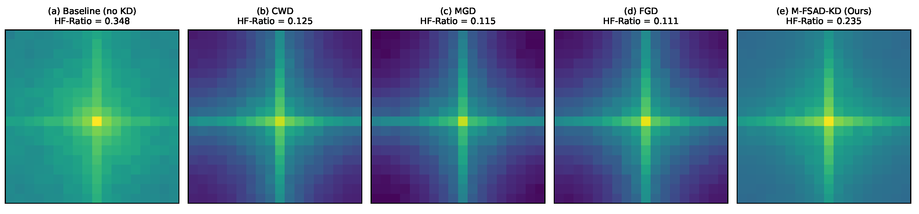
Spectral excess in the SAR-only baseline (Figure 4). The teacher–student comparison confirms that the SAR-only baseline carries a measurable high-frequency excess relative to the multi-modal teacher: the high-frequency energy ratio (HF-Ratio, defined as the fraction of ${\left|\mathcal{F}\right|}^2$ energy beyond the cutoff radius ${\sigma }_f=min(H,W)/4$) is $0.348$ for the baseline against $0.319$ for the teacher. The difference panel localizes the excess in the band where SAR speckle dominates. This is the precondition for the trap: the SAR-only student carries broadband high-frequency content that the optical-fused teacher has filtered out.

Indiscriminate over-suppression by spatial-distance distillation (Figure 5). Comparing the P4 spectrum of the student trained under each method reveals a sharp asymmetry. Spatial-distance-based methods drive the HF-Ratio far below the teacher reference: CWD collapses to $0.125$, MGD to $0.115$, and FGD to $0.111$—roughly one-third of the teacher’s $0.319$. Without a frequency-aware gating mechanism, these losses force the student to indiscriminately suppress all high-frequency content, including the target-edge information that small-object detection relies on. The empirical consequence is the storage-tank AP collapse observed under CWD (9.85% vs. baseline 11.4%). M-FSAD-KD’s HF-Ratio of $0.235$, by contrast, sits in the operating regime between the over-suppressed trap methods and the noise-loaded baseline ($0.348$), demonstrating that the frequency-decoupled loss retains target-relevant high-frequency content rather than collapsing the band entirely.

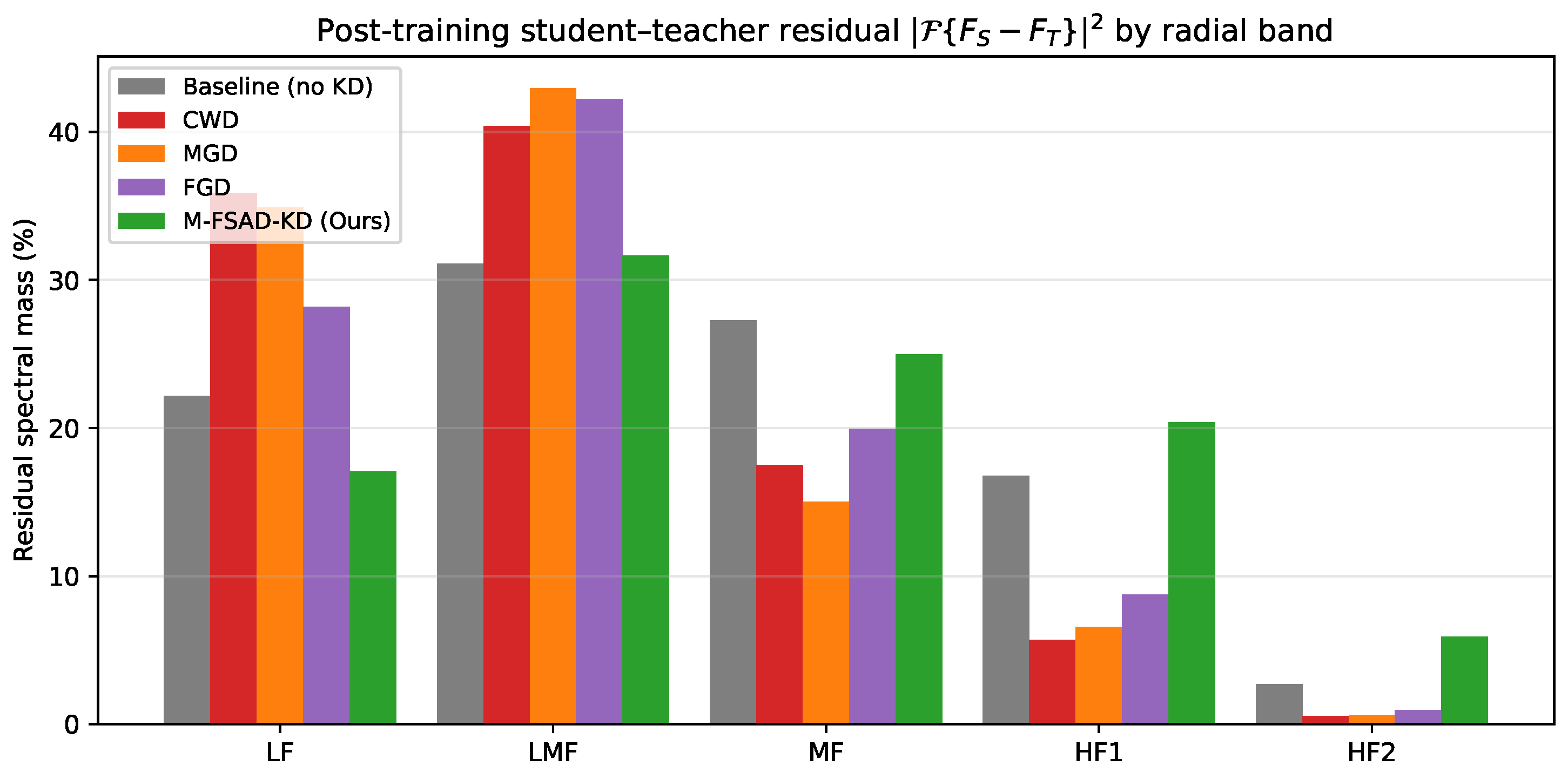
Low-frequency alignment versus high-frequency freedom (Figure 6). To localize where each method’s alignment succeeds, we decompose the channel-averaged, L2-normalized student–teacher residual ${\overline{F}}_S-{\overline{F}}_T$ into five equal-width radial frequency bands (LF, LMF, MF, HF1, HF2). Two patterns are diagnostic. The trap methods concentrate the post-training residual in the low-frequency end: LF + LMF accounts for $76\%$, $78\%$, and $70\%$ of CWD’s, MGD’s, and FGD’s residual energy, respectively, while their HF1 + HF2 residual share falls below $10\%$ in all three cases. The student matches the teacher in HF only by sending its HF content close to zero—a vacuous form of alignment. M-FSAD-KD, by contrast, achieves the smallest LF residual share among all methods ($0.171$, against $0.222$ for the baseline, $0.359$ for CWD, $0.349$ for MGD, and $0.282$ for FGD), with the residual energy more evenly distributed across bands (LF + LMF $=49\%$, MF + HF1 + HF2 $=51\%$). The Gaussian low-pass mask in M-FSAD-KD concentrates the alignment budget in the structural low-frequency band where teacher and student should agree, while leaving the high-frequency band as a degree of freedom for the SAR-only student to retain its own target-edge content; consistent with the mask ablation (Table 5), this reflects amplitude-domain alignment rather than any specific low-pass shape.

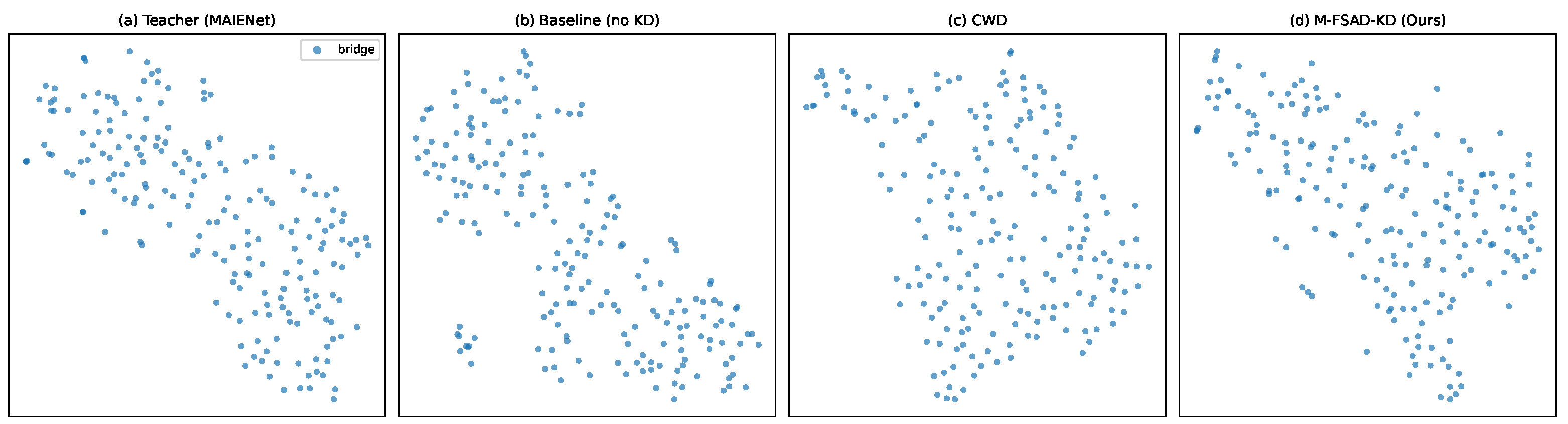
Manifold recovery (Figure 7). Two-dimensional t-SNE projections of channel-averaged P4 features corroborate the spectral picture in the embedding space. Under the multi-modal teacher, the three target classes form well-separated clusters; under the non-distilled baseline, the clusters partially overlap; under CWD, cluster identity is further degraded, consistent with the over-suppression hypothesis; under M-FSAD-KD, the cluster geometry approaches the teacher’s, with cleaner inter-class margins than either the baseline or CWD.

Synthesis. The four diagnostics jointly establish a coherent physical picture of the speckle-fitting trap. The unimodal SAR student inherits a measurable high-frequency excess (Figure 4); spatial-distance distillation methods respond by indiscriminately collapsing the high-frequency band, simultaneously erasing the target-edge content needed for small-object detection (Figure 5); the resulting student matches the teacher in HF only by sending its HF content close to zero, leaving the structural low-frequency band poorly aligned (Figure 6) and the feature manifold loses inter-class separability (Figure 7). M-FSAD-KD’s frequency-decoupled distillation reverses each of these signatures: it preserves target-relevant high-frequency content rather than collapsing it, achieves the smallest low-frequency residual among all methods, and recovers a teacher-like cluster geometry. Together, these results provide direct physical support for the formal gradient-domain analysis in Section 3.8.

4.5. Ablation Study

Table 7. Full-link ablation of M-FSAD-KD components (100 epochs, student YOLOv11n*, single hardware platform). A checkmark (✓) indicates that the corresponding component (Bk, Freq, JSCAD, or KD) is enabled in that configuration; an empty cell means it is disabled. All rows are single representative runs measured under identical conditions, so the within-table differences isolate each component’s contribution; the $49.7\%$ full-model entry is the best of these runs, whose multi-seed mean ± std is $47.9\pm 0.9$ (Table 3). Best results in each column are in bold.

Bk	Freq	JSCAD	KD	${\mathbf{AP}}_{\mathbf{Bri}.}$	${\mathbf{AP}}_{\mathbf{Har}.}$	${\mathbf{AP}}_{\mathbf{Tan}.}$	${\mathbf{mAP}}_{50}$	${\mathbf{mAP}}_{50:95}$
				44.1	75.3	11.4	43.6	22.9
	✓			44.4	73.9	12.1	43.4	22.9
		✓		44.6	73.0	12.4	43.4	22.5
			✓	48.2	84.1	13.1	48.4	26.3
✓				47.4	79.3	13.6	46.8	25.2
✓		✓		47.3	79.2	13.7	46.7	25.0
✓	✓			47.2	81.1	13.6	47.3	25.7
✓	✓	✓		47.7	83.3	12.3	47.8	26.5
✓	✓	✓	✓	48.6	86.5	14.0	49.7	28.3

dissects the interaction among the four granularities. Three observations emerge.

Feature-manifold alignment is a prerequisite. Without Bk, applying Freq or JSCAD alone leaves the student at the baseline level (43.4% and 43.4% vs. 43.6%), whereas introducing Bk alone lifts the student to 46.8% ($+3.2$ absolute points). Without a shared channel layout, the teacher–student distance in feature space is geometrically ill-posed, and any subsequent frequency- or attention-based gating cannot take effect; Bk supplies the channel alignment that enables the downstream components to act.

Freq and JSCAD are jointly active rather than individually additive. Adding JSCAD alone on top of Bk leaves accuracy essentially unchanged (46.7% vs. 46.8%), and adding Freq alone on top of Bk yields only a marginal lift to 47.3% ($+0.5$ absolute points). Co-deploying both reaches 47.8% ($+1.0$ absolute points over Bk-alone)—a combined gain that exceeds the sum of individual contributions. Frequency decoupling supplies a low-noise substrate on which the joint spatial–channel attention can focus correctly; in isolation, each component lacks the partner that converts its mechanism into accuracy.

Response-level KD is additive on top of the purified feature manifold. Stacking head-end KD on top of the full M-FSAD branch lifts ${\mathrm{mAP}}_{50}$ from 47.8% to 49.7% ($+1.9$ absolute points) and ${\mathrm{mAP}}_{50:95}$ from 26.5% to 28.3% ($+1.8$ absolute points), showing that the head-end calibration of soft labels remains valuable even after the feature manifold has been purified. The full configuration achieves the best AP in every column.

4.6. Loss-Weight Sensitivity

We perform a one-factor-at-a-time sweep over the four weights to characterize their sensitivity (

Table 8. Sensitivity sweep of distillation weights (baseline ${\lambda }_{\mathrm{bk}}=100.0$). All configurations are single representative runs under identical conditions; the multi-seed mean ± std of the deployed configuration is $47.9\pm 0.9$ (Table 3), so the absolute values sit at the upper end of the seed distribution while the within-sweep trends isolate each weight’s effect. Best results in each group are in bold.

Distillation Weight Configuration			Per-Class AP (%)			Overall Metric (%)
${\mathbf{\lambda }}_{\mathrm{freq}}$	${\mathbf{\lambda }}_{\mathrm{jscad}}$	${\mathbf{\lambda }}_{\mathrm{kd}}$	${\mathbf{AP}}_{\mathbf{Bri}.}$	${\mathbf{AP}}_{\mathbf{Har}.}$	${\mathbf{AP}}_{\mathbf{Tan}.}$	${\mathbf{mAP}}_{\mathbf{50}}$	${\mathbf{mAP}}_{\mathbf{50}:\mathbf{95}}$
Group I: Probing the Freq decoupling weight (${\lambda }_{\mathrm{jscad}}=10.0,{\lambda }_{\mathrm{kd}}=0.12$)
20.0	10.0	0.12	48.9	83.3	14.4	48.9	26.8
45.0 (baseline)	10.0	0.12	48.7	85.0	12.3	48.7	27.0
80.0	10.0	0.12	48.6	86.5	14.0	49.7	28.3
120.0	10.0	0.12	49.0	84.9	13.4	49.1	27.1
Group II: Searching the JSCAD weight (${\lambda }_{\mathrm{freq}}=45.0,{\lambda }_{\mathrm{kd}}=0.12$)
45.0	5.0	0.12	48.7	84.4	13.6	48.9	27.3
45.0	10.0 (baseline)	0.12	48.7	85.0	12.3	48.7	27.0
45.0	20.0	0.12	48.5	84.6	13.1	48.7	27.3
Group III: Probing the response-level boundary (${\lambda }_{\mathrm{freq}}=45.0,{\lambda }_{\mathrm{jscad}}=10.0$)
45.0	10.0	0.05	48.2	83.3	15.0	48.8	26.8
45.0	10.0	0.12 (baseline)	48.7	85.0	12.3	48.7	27.0
45.0	10.0	0.25	49.3	85.0	13.6	49.3	27.3
45.0	10.0	0.50	49.1	86.8	12.8	49.6	26.9
Group IV: Joint extrema
80.0	5.0	0.25	49.5	85.8	11.4	48.9	27.1

). Three regularities are noteworthy.

Critical effect of frequency decoupling. In Group I, increasing ${\lambda }_{\mathrm{freq}}$ from 45.0 to 80.0 raises ${\mathrm{mAP}}_{50}$ from 48.7% to 49.7% and lifts the harbor AP from 85.0% to 86.5%, indicating that stronger frequency suppression further removes shoreline clutter. Further increasing ${\lambda }_{\mathrm{freq}}$ to 120.0 reduces ${\mathrm{mAP}}_{50}$ back to 49.1%, showing that excessive frequency constraint over-smooths the high-frequency edges of target bodies.

Scale-balance trade-off triggered by logit constraint. In Group III, as ${\lambda }_{\mathrm{kd}}$ rises from 0.05 to 0.50, the harbor AP (large-scale class) rises from 83.3% to 86.8% and the overall ${\mathrm{mAP}}_{50}$ rises from 48.8% to 49.6%, while the oil-tank AP (small-scale class) drops from 15.0% to 12.8%. A stronger logit constraint pulls the student toward the teacher’s large-scale feature distribution, whereas a weaker constraint preserves the freedom of low-level responses and benefits the self-driven discovery of micro-target features.

Non-linear coupling under joint extrema. Group IV combines the single-axis extrema (Freq $=80.0$, JSCAD $=5.0$, KD $=0.25$). This combination reduces ${\mathrm{mAP}}_{50}$ to 48.9% and further reduces the oil-tank AP to 11.4%, showing that stacking strong constraints over-restricts the feature response space. The total improvement is, therefore, not a linear superposition of single-axis gains; under the present search range, the Group I configuration (${\lambda }_{\mathrm{freq}}=80.0,{\lambda }_{\mathrm{jscad}}=10.0,{\lambda }_{\mathrm{kd}}=0.12$) is the empirically optimal operating point.

4.7. Full-Convergence Deployment Evaluation

To establish the upper performance bound, we retrain both a lightweight (YOLOv11n*) and a mid-capacity (YOLOv11m*) student under the best weight configuration for 40 epochs (

Table 9. Deployment-level performance at 400 epochs. Best result in each column is in bold.

Model	Modality/Role	Params (M)	GFLOPs (G)	${\mathbf{AP}}_{\mathbf{Bri}.}$	${\mathbf{AP}}_{\mathbf{Har}.}$	${\mathbf{AP}}_{\mathbf{Tan}.}$	${\mathbf{mAP}}_{50}$ (%)
MAIENet (Teacher)	Multi-modal (SAR + Optical)	34.00	27.60	93.8	99.4	79.0	90.8
Baseline (YOLOv11n*)	Single-modal SAR (no KD)	2.39	1.29	57.4	94.0	21.8	57.7
Baseline (YOLOv11m*)	Single-modal SAR (no KD)	19.98	15.32	76.4	98.7	47.0	74.0
M-FSAD-KD (YOLOv11n*)	Single-modal SAR (full-link distillation)	2.39	1.29	64.9	97.6	20.8	61.1
M-FSAD-KD (YOLOv11m*)	Single-modal SAR (full-link distillation)	19.98	15.32	90.1	99.5	56.2	81.9

).

At 2.39 M parameters, M-FSAD-KD lifts ${\mathrm{mAP}}_{50}$ from 57.7% to 61.1%, a gain of 3.4 absolute points. At 19.98 M parameters, it lifts the student from 74.0% to 81.9%, a gain of 7.9 absolute points. The harbor AP of the mid-capacity student reaches 99.5%, matching the teacher’s 99.4% on this near-saturated class (a 0.1-point difference that lies within run-to-run variance). We attribute the residual gap of 8.9 absolute points between the mid-capacity student and the teacher largely to the information asymmetry between a single SAR band and the optical band; we do not claim this is an exactly quantifiable physical limit, and narrowing it further is left to future work.

4.8. Feature Manifold Evolution and Interpretability Analysis

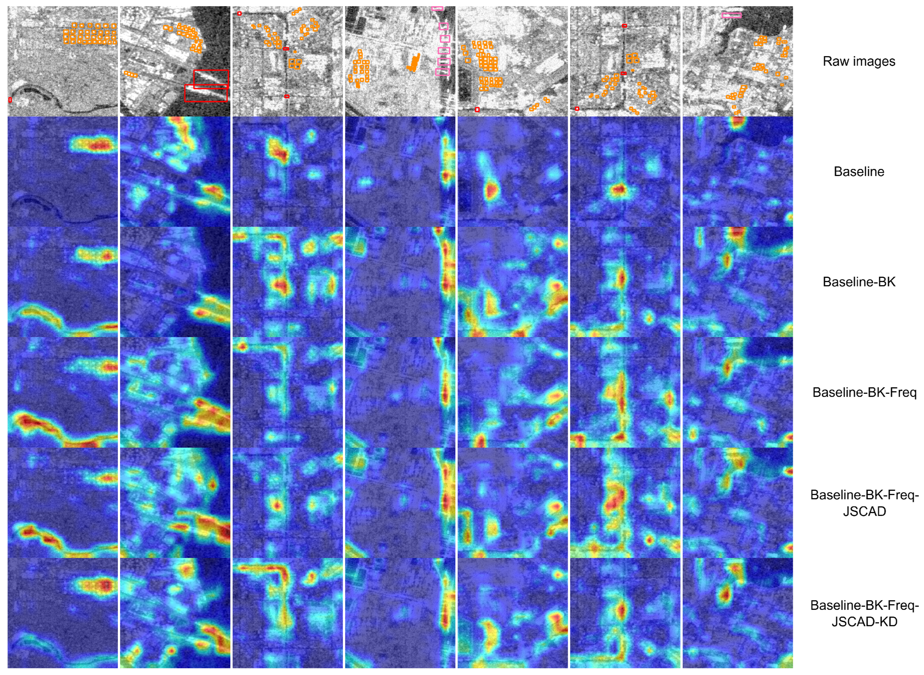
To examine how the distillation chain reshapes the latent space, we extract P4 activation maps along the cumulative module sequence (baseline →+Bk →+Bk + Freq →+Bk + Freq + JSCAD → full M-FSAD-KD) and visualize them as energy heatmaps in Figure 8.

Three patterns emerge. (1) Correction of context bias. In scenes containing tiny bridges over narrow rivers, the SAR-only baseline responds weakly to the bridges, and intermediate configurations transfer some response onto the continuous water body, producing a context-correlated spurious activation. Once the response-level KD is included, the residual high-frequency response on the water body is suppressed and the activation concentrates on the bridge itself, indicating that feature-level alignment establishes the structural backbone of the response while head-level KD refines its boundary. (2) Regional aggregation in dense scenes. For dense harbor and oil-tank regions, the P4 receptive field exceeds individual target footprints, and the high-frequency responses of clustered instances merge into a single semantically coherent region, providing a regional proposal that decouples instance separation from the regression branch. (3) Weak-target preservation. For isolated micro-scale oil tanks, the frequency-decoupled component induces mild low-pass smoothing at the target edge. The full M-FSAD-KD configuration nevertheless retains a distinguishable activation on the target, indicating that the joint spatial–channel attention compensates for the unavoidable smoothing introduced by frequency gating.

4.9. Cross-Method Detection Comparison and Convergence Dynamics

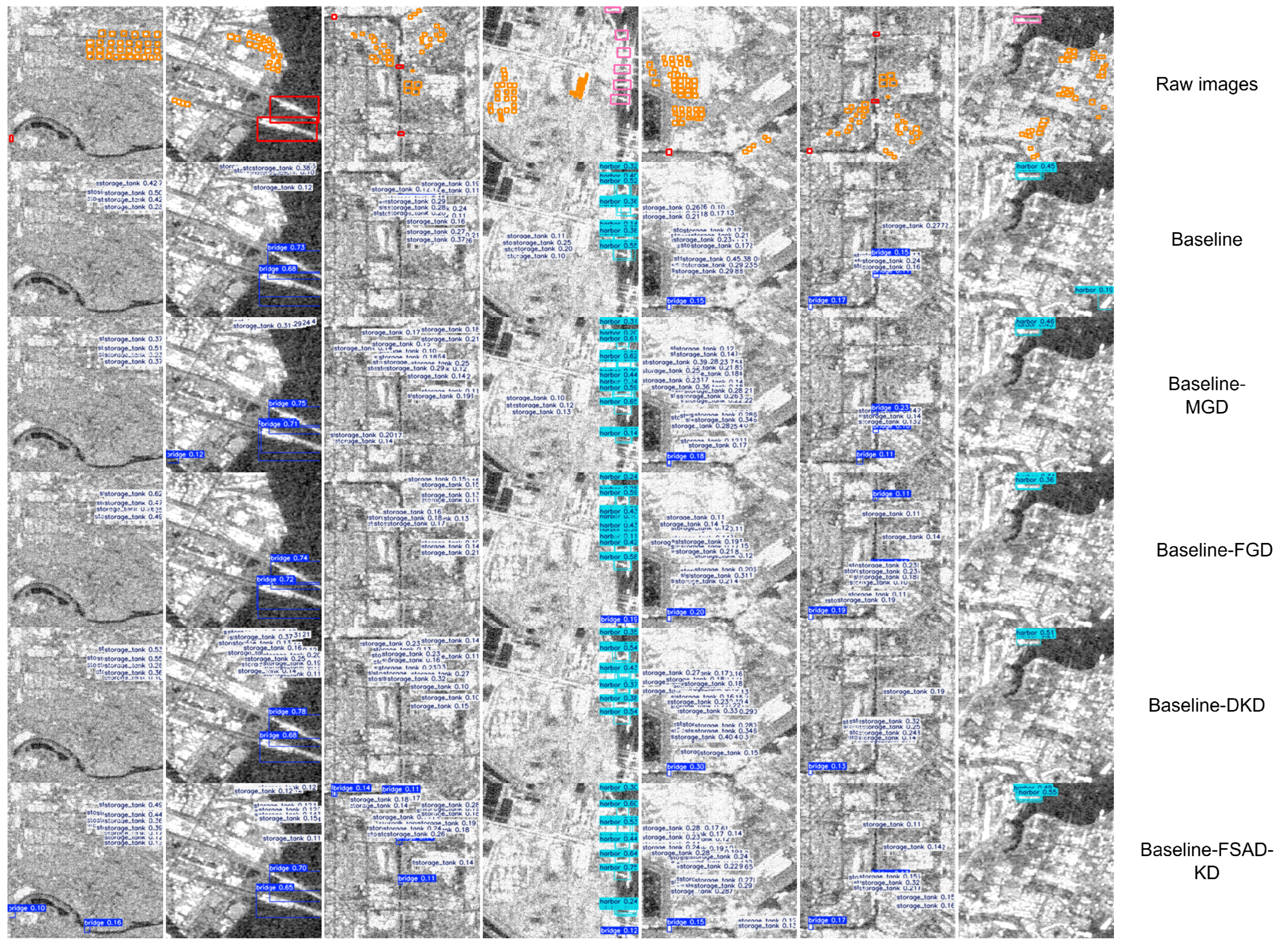
We select complex maritime and dense industrial scenes for qualitative comparison. Figure 9 shows the detection results of the baseline, feature-level representatives (MGD, FGD), the response-level representative (DKD), and M-FSAD-KD.

The qualitative comparison reveals the per-method failure modes. The baseline produces context-biased predictions and false alarms on shoreline structures. MGD partially suppresses background activations but retains residual class confusion in dense regions. DKD, which operates only at the head end, has no mechanism to purify low-level features and remains sensitive to speckle-driven false positives. M-FSAD-KD removes the context-correlated spurious responses and reduces false alarms across both maritime and industrial scenes; the residual misses on the smallest isolated oil tanks are consistent with the quantitative analysis and reflect the trade-off between high-frequency denoising and large-scale alignment under a tight parameter budget.

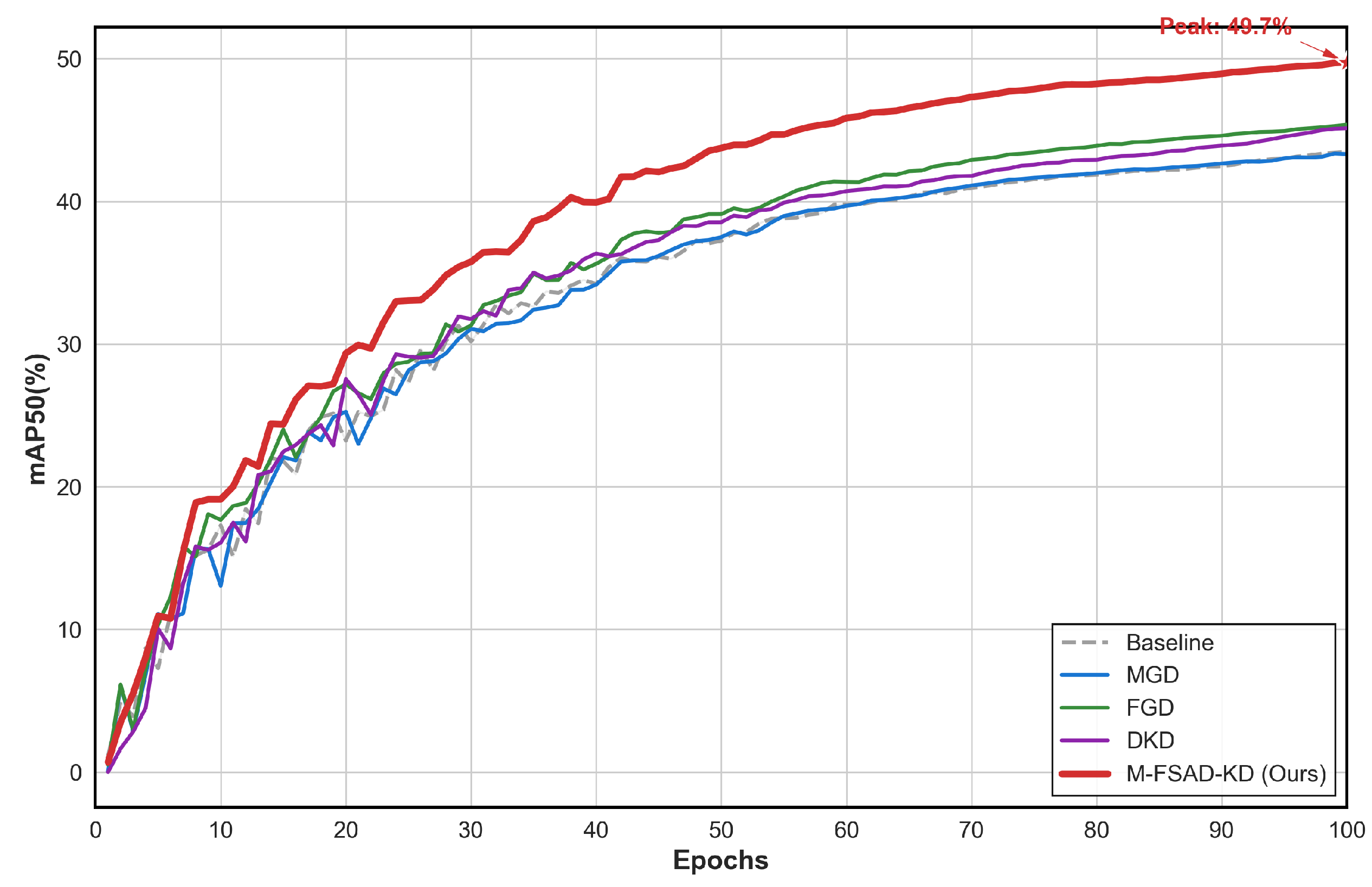
Figure 10 plots the ${\mathrm{mAP}}_{50}$ convergence dynamics over the first 100 training epochs.

In the early stage (epochs 0–20), the SAR-only baseline converges slowly under the cross-modal gap; M-FSAD-KD, supported by frequency decoupling and joint spatial–channel mask focusing, follows a steeper trajectory. In the middle stage (epochs 20–60), the curves of MGD and DKD flatten as their alignment paths saturate, whereas M-FSAD-KD maintains a steady gain (reaching 45.8% at epoch 60). In the late stage (epochs 60–100), M-FSAD-KD converges to 49.7%, exceeding the baseline by 6.1 absolute points and demonstrating that the full-link configuration both accelerates convergence and raises the achievable upper bound.

5. Discussion

The experimental results confirm that M-FSAD-KD counteracts the speckle-fitting trap in cross-modal SAR distillation. We discuss four observations below.

First, the ablation in Section 4 establishes feature-manifold alignment (Bk) as a prerequisite for feature-level distillation in the heterogeneous-modality regime: applying Freq or JSCAD without Bk leaves the student at the baseline level, whereas Bk alone lifts the student by $3.2$ absolute points. This is consistent with the LUPI principle that privileged information must first be projected into a manifold compatible with the student’s representational basis before any structural alignment can take effect.

Second, the comparison with feature-level baselines validates the speckle-fitting-trap diagnosis. CWD degrades the student below the non-distilled baseline (42.2% vs. 43.6% ${\mathrm{mAP}}_{50}$), with the impact concentrated on the smallest-target storage-tank class (9.85% vs. baseline 11.4%, and a near-zero AP of 0.10% on an independently trained run on separate hardware). Such a degradation pattern is rarely reported in homogeneous-modality KD literature and indicates that the conventional assumption of a quasi-homogeneous teacher–student manifold breaks down once SAR speckle enters the alignment loss. The Part C spectral and manifold diagnostics in Section 4.4.3 localize the mechanism: trap-affected methods collapse the high-frequency band indiscriminately, eroding both speckle and target-edge content, while M-FSAD-KD’s frequency-decoupled gating preserves the target-edge band and aligns the structural low-frequency band.

Third, the cross-teacher-architecture validation in Section 4.4.2 establishes that the framework is not specific to MAIENet. Swapping the teacher for DEYOLO—a dual-stream YOLOv8-based detector that differs from MAIENet in backbone family, stream topology, and fusion location—retains 48.6% ${\mathrm{mAP}}_{50}$ at the student, within 1.1 absolute points of the MAIENet result. Disabling Bk under DEYOLO drops the result by 2.3 absolute points but still exceeds the baseline by 2.7 absolute points, so even the operator-level adapter transfers across architecture families. This suggests the framework can be paired with other sufficiently strong multi-modal SAR–optical teachers without per-teacher re-engineering, though we bound this claim to the two architecture families tested pending broader validation.

Fourth, the deployment evaluation shows that the framework scales positively with student capacity: a 2.39 M student gains 3.4 absolute points, and a 19.98 M student gains 7.9 absolute points relative to their respective non-distilled baselines. The harbor AP of the mid-capacity student matches the multi-modal teacher on this near-saturated class (99.5% vs. 99.4%, within run-to-run variance). We attribute the residual gap of 8.9 absolute points to the teacher on overall ${\mathrm{mAP}}_{50}$ largely to the information asymmetry between a single SAR band and the optical band, rather than to a strictly quantifiable physical limit.

Several boundaries delimit the present study and indicate clear directions for future work. First, the Gaussian bandwidth ${\sigma }_f=min(H,W)/4$ is a fixed empirical setting; targets with prominent high-frequency geometry (for example, wake patterns and densely packed micro-targets) may suffer mild edge over-smoothing. Learning ${\sigma }_f$ in a data-driven manner is a natural extension. Second, two design choices are heuristic and worth flagging explicitly: (i) the JSCAD mask is derived from teacher activations and, therefore, inherits any teacher over-activation or class bias—entropy-aware gating that down-weights over-confident teacher regions is a natural mitigation and (ii) the four loss weights are fixed after a single first-epoch gradient-norm calibration (100:80:10:0.12) rather than re-estimated per batch, which avoids per-batch or hardware sensitivity of the deployed weights but remains a heuristic—replacing it with a principled uncertainty-weighted (homoscedastic) balancing scheme is a promising alternative. We also note that, consistent with the multi-seed variance reported in Section 4, the deployed configuration is stable across independent runs. Third, M-FSAD-KD still requires rigorously co-registered SAR–optical pairs at training time; semi-supervised extensions to partially paired data are an open direction. Fourth, cross-dataset and cross-modal empirical validation is left as future work. The theoretical analysis in Section 3.8 (Generality) suggests that the framework should extend to other modality pairs satisfying the low-frequency-signal–wide-band-noise hypothesis, such as RGB–infrared, RGB–depth, or visible–hyperspectral pairs; empirical verification on these benchmarks requires a matching multi-modal teacher to be pre-trained on the target paired data and is deferred to subsequent studies. Fifth, broader benchmarking on additional SAR detection datasets beyond OGSOD-1.0 is also left to future work; together with the cross-modal extension above, it would tighten the empirical evidence for the generality claimed by the present theoretical analysis.

6. Conclusions

This paper presented M-FSAD-KD, a full-link multi-granularity distillation framework for cross-modal SAR object detection under optical-modality absence. Its starting point is a diagnosis: the leading channel-wise feature distillation (CWD) degrades a SAR-only student below the non-distilled baseline, with small-target AP collapsing—a failure mode we name the speckle-fitting trap, formalized through a gradient-domain analysis (Section 3.8), and verified through spectral and feature-manifold diagnostics (Section 4.4.3). To avoid the trap, the framework integrates a shallow backbone adapter (Bk), a neck-stage frequency-decoupled distillation (Freq), a mid-level joint spatial–channel attention distillation (JSCAD), and an end-stage response-level calibration (KD), coordinated under a dimensional-homogenization weight scheme. Its key methodological novelty is the frequency-decoupled formulation: a dynamic Gaussian low-pass mask applied to the teacher–student amplitude-spectrum alignment loss, which transfers low-frequency structural content while—unlike the channel-wise softmax alignment that triggers the trap—leaving the student free to retain its own target-edge high-frequency band rather than being forced onto the broadband speckle profile. Consistent with the mask ablation (Table 5), this benefit stems from aligning in the amplitude-spectrum domain rather than from any specific low-pass shape. On OGSOD-1.0, M-FSAD-KD outperforms strong distillation baselines at both 2.39 M and 19.98 M student capacities, lifts the mid-capacity student to within 8.9 absolute points of the multi-modal teacher under SAR-only inference, and transfers across teacher architecture families, as validated on the single-stream MAIENet and the dual-stream DEYOLO teachers in Section 4.4.2.

Future work will pursue four directions: (i) learnable frequency-domain bandwidths that adapt ${\sigma }_f$ to per-scene statistics rather than fixing it empirically; (ii) mitigation of the teacher-bias inheritance carried by the JSCAD mask; (iii) extension to semi-supervised settings where SAR–optical pairs are only partially available and (iv) empirical validation on additional SAR detection benchmarks and on cross-modal scenarios beyond SAR–optical (RGB–infrared, RGB–depth, and visible–hyperspectral), which would substantiate the theoretical generality argued in Section 3.8.

References

1. Moreira, A.; Prats-Iraola, P.; Younis, M.; Krieger, G.; Hajnsek, I.; Papathanassiou, K.P. A tutorial on synthetic aperture radar. IEEE Geosci. Remote Sens. Mag. 2013, 1, 6–43. [Google Scholar] [CrossRef] [Scilit]
2. Zhao, C.; Fu, X.; Dong, J.; Cao, S.; Zhang, C. Enhancing, Refining, and Fusing: Towards Robust Multiscale and Dense Ship Detection. IEEE J. Sel. Top. Appl. Earth Obs. Remote Sens. 2025, 18, 9919–9933. [Google Scholar] [CrossRef] [Scilit]
3. Liu, S.; Gao, L.; Lei, Y.; Wang, M.; Hu, Q.; Ma, X.; Zhang, Y.D. SAR Speckle Removal Using Hybrid Frequency Modulations. IEEE Trans. Geosci. Remote Sens. 2021, 59, 3956–3966. [Google Scholar] [CrossRef] [Scilit]
4. Gui, S.; Song, S.; Qin, R.; Tang, Y. Remote Sensing Object Detection in the Deep Learning Era—A Review. Remote Sens. 2024, 16, 327. [Google Scholar] [CrossRef] [Scilit]
5. Wang, C.; Ruan, R.; Zhao, Z.; Li, C.; Tang, J. Category-oriented localization distillation for SAR object detection and a unified benchmark. IEEE Trans. Geosci. Remote Sens. 2023, 61, 5211314. [Google Scholar] [CrossRef] [Scilit]
6. Tong, Y.; Xiong, K.; Liu, J.; Cao, G.; Fan, X. MAIENet: Multi-Modality Adaptive Interaction Enhancement Network for SAR Object Detection. Remote Sens. 2025, 17, 3866. [Google Scholar] [CrossRef] [Scilit]
7. Li, J.; Hong, D.; Gao, L.; Yao, J.; Zheng, K.; Zhang, B.; Chanussot, J. Deep learning in multimodal remote sensing data fusion: A comprehensive review. Int. J. Appl. Earth Obs. Geoinf. 2022, 112, 102926. [Google Scholar] [CrossRef] [Scilit]
8. Wei, S.; Luo, C.; Luo, Y. MMANet: Margin-aware distillation and modality-aware regularization for incomplete multimodal learning. In Proceedings of the IEEE/CVF Conference on Computer Vision and Pattern Recognition (CVPR), Vancouver, BC, Canada, 17–24 June 2023; IEEE: New York, NY, USA, 2023; pp. 20039–20049. [Google Scholar]
9. Vapnik, V.; Izmailov, R. Learning using privileged information: Similarity control and knowledge transfer. J. Mach. Learn. Res. 2015, 16, 2023–2049. [Google Scholar]
10. Gupta, S.; Hoffman, J.; Malik, J. Cross modal distillation for supervision transfer. In Proceedings of the IEEE Conference on Computer Vision and Pattern Recognition (CVPR), Las Vegas, NV, USA, 27–30 June 2016; IEEE: New York, NY, USA, 2016; pp. 2827–2836. [Google Scholar]
11. Hinton, G.; Vinyals, O.; Dean, J. Distilling the knowledge in a neural network. In Proceedings of the NIPS Deep Learning and Representation Learning Workshop, Montreal, QC, Canada, 11–12 December 2015. [Google Scholar]
12. Chen, G.; Choi, W.; Yu, X.; Han, T.; Chandraker, M. Learning efficient object detection models with knowledge distillation. In Proceedings of the Advances in Neural Information Processing Systems (NeurIPS), Long Beach, CA, USA, 4–9 December 2017; Volume 30. [Google Scholar]
13. Chen, Y.; Wang, B.; Guo, X.; Zhu, W.; He, J.; Liu, X.; Yuan, J. DEYOLO: Dual-feature-enhancement YOLO for cross-modality object detection. In Proceedings of the International Conference on Pattern Recognition, Kolkata, India, 1–5 December 2024; pp. 236–252. [Google Scholar]
14. Song, K.; Xue, X.; Wen, H.; Ji, Y.; Yan, Y.; Meng, Q. Misaligned visible-thermal object detection: A drone-based benchmark and baseline. IEEE Trans. Intell. Veh. 2024, 9, 7449–7460. [Google Scholar] [CrossRef] [Scilit]
15. Shen, J.; Chen, Y.; Liu, Y.; Zuo, X.; Fan, H.; Yang, W. ICAFusion: Iterative cross-attention guided feature fusion for multispectral object detection. Pattern Recognit. 2024, 145, 109913. [Google Scholar] [CrossRef] [Scilit]
16. Cao, Y.; Bin, J.; Hamari, J.; Blasch, E.; Liu, Z. Multimodal object detection by channel switching and spatial attention. In Proceedings of the IEEE/CVF Conference on Computer Vision and Pattern Recognition Workshops (CVPRW), Vancouver, BC, Canada, 17–24 June 2023; IEEE: New York, NY, USA, 2023; pp. 403–411. [Google Scholar] [CrossRef] [Scilit]
17. Gou, J.; Yu, B.; Maybank, S.J.; Tao, D. Knowledge Distillation: A Survey. Int. J. Comput. Vis. 2021, 129, 1789–1819. [Google Scholar] [CrossRef] [Scilit]
18. Romero, A.; Ballas, N.; Kahou, S.E.; Chassang, A.; Gatta, C.; Bengio, Y. FitNets: Hints for thin deep nets. In Proceedings of the International Conference on Learning Representations (ICLR), San Diego, CA, USA, 7–9 May 2015. [Google Scholar]
19. Yang, Z.; Li, Z.; Jiang, X.; Gong, Y.; Yuan, Z.; Zhao, D.; Yuan, C. Focal and Global Knowledge Distillation for Detectors. In Proceedings of the IEEE/CVF Conference on Computer Vision and Pattern Recognition (CVPR), New Orleans, LA, USA, 18–24 June 2022; IEEE: New York, NY, USA, 2022; pp. 4643–4652. [Google Scholar]
20. Yang, Z.; Li, Z.; Shao, M.; Shi, D.; Yuan, Z.; Yuan, C. Masked Generative Distillation. In Proceedings of the European Conference on Computer Vision (ECCV); Springer: Berlin/Heidelberg, Germany, 2022; pp. 53–69. [Google Scholar]
21. Zheng, Z.; Ye, R.; Wang, P.; Ren, D.; Zuo, W.; Hou, Q.; Cheng, M.M. Localization distillation for dense object detection. In Proceedings of the IEEE/CVF Conference on Computer Vision and Pattern Recognition (CVPR), New Orleans, LA, USA, 18–24 June 2022; IEEE: New York, NY, USA, 2022; pp. 9397–9406. [Google Scholar]
22. Zhao, B.; Cui, Q.; Song, R.; Qiu, Y.; Liang, J. Decoupled knowledge distillation. In Proceedings of the IEEE/CVF Conference on Computer Vision and Pattern Recognition (CVPR), New Orleans, LA, USA, 18–24 June 2022; IEEE: New York, NY, USA, 2022; pp. 11943–11952. [Google Scholar]
23. Shu, C.; Liu, Y.; Gao, J.; Yan, Z.; Shen, C. Channel-wise knowledge distillation for dense prediction. In Proceedings of the IEEE/CVF International Conference on Computer Vision (ICCV), Montreal, QC, Canada, 10–17 October 2021; IEEE: New York, NY, USA, 2021; pp. 5311–5320. [Google Scholar]
24. Dai, X.; Jiang, Z.; Wu, Z.; Bao, Y.; Wang, Z.; Liu, S.; Zhou, E. General instance distillation for object detection. In Proceedings of the IEEE/CVF Conference on Computer Vision and Pattern Recognition (CVPR), Nashville, TN, USA, 20–25 June 2021; IEEE: New York, NY, USA, 2021; pp. 7838–7847. [Google Scholar]
25. Xu, K.; Qin, M.; Sun, F.; Wang, Y.; Chen, Y.K.; Ren, F. Learning in the frequency domain. In Proceedings of the IEEE/CVF Conference on Computer Vision and Pattern Recognition (CVPR), Seattle, WA, USA, 13–19 June 2020; IEEE: New York, NY, USA, 2020; pp. 1740–1749. [Google Scholar]
26. He, K.; Chen, X.; Xie, S.; Li, Y.; Dollár, P.; Girshick, R. Masked autoencoders are scalable vision learners. In Proceedings of the IEEE/CVF Conference on Computer Vision and Pattern Recognition (CVPR), New Orleans, LA, USA, 18–24 June 2022; IEEE: New York, NY, USA, 2022; pp. 16000–16009. [Google Scholar]
27. Khanam, R.; Hussain, M. YOLOv11: An overview of the key architectural enhancements. arXiv 2024, arXiv:2410.17725. [Google Scholar]
28. Lin, T.Y.; Maire, M.; Belongie, S.; Hays, J.; Perona, P.; Ramanan, D.; Dollár, P.; Zitnick, C.L. Microsoft COCO: Common objects in context. In Proceedings of the European Conference on Computer Vision (ECCV), Zurich, Switzerland, 6–12 September 2014; pp. 740–755. [Google Scholar]
29. Wei, S.; Luo, C.; Luo, Y. Scale Decoupled Distillation. In Proceedings of the IEEE/CVF Conference on Computer Vision and Pattern Recognition (CVPR), Seattle, WA, USA, 17–21 June 2024; IEEE: New York, NY, USA, 2024; pp. 15975–15983. [Google Scholar]
30. Sun, S.; Ren, W.; Li, J.; Wang, R.; Cao, X. Logit Standardization in Knowledge Distillation. In Proceedings of the IEEE/CVF Conference on Computer Vision and Pattern Recognition (CVPR), Seattle, WA, USA, 17–21 June 2024; IEEE: New York, NY, USA, 2024; pp. 15731–15740. [Google Scholar]
31. Xu, L.; Liu, K.; Liu, J.; Wang, L.; Xu, L.; Cheng, J. Local Dense Logit Relations for Enhanced Knowledge Distillation. In Proceedings of the IEEE/CVF International Conference on Computer Vision (ICCV), Honolulu, Hawaii, USA, 19–23 October 2025; IEEE: New York, NY, USA, 2025. [Google Scholar]
Figure 1. Overall architecture of the proposed M-FSAD-KD framework.
Remotesensing 18 03008 g001
Figure 2. Step-by-step walkthrough of frequency-decoupled distillation on a real OGSOD-1.0 optical–SAR scene. (a) Optical image (teacher-only, privileged information). (b) SAR image (student input); the red box marks a speckle/clutter region magnified in (b’). (c) 2D Fourier log-amplitude spectrum of the SAR image: structure concentrates at low frequency, speckle spreads across the high-frequency plane. (d) Dynamic Gaussian low-pass gate M freq with σ f = min ( H , W ) / 4 . (e) Low-frequency component retained by the gate—the structural information transferred to the student. (f) Complementary high-frequency component—target edges mixed with speckle—which carries no alignment gradient and is left free for the student to keep. (g) M-FSAD-KD detection result on the same scene.
Remotesensing 18 03008 g002
Figure 3. Empirical support for the additive and wide-band assumptions, measured on the non-distilled SAR-only student (Monte-Carlo over 16 speckle realizations of 50 OGSOD-1.0 SAR images, single-look L = 1 ). (a) The speckle-induced feature noise-variance ratio E [ N 2 ] / E [ S 2 ] falls from ≈0.44 at shallow backbone layers to ≈0.02 at the deepest layer, so the first-order additive approximation of Equation (14) becomes increasingly accurate at the deep stages where distillation operates. (b) Radial power spectrum of the fluctuation N by depth: at the shallow-to-mid stages (layers 2, 4, 6) the perturbation is wide-band (≈60– 63 % of its power beyond normalized radial frequency 0.2 , consistent with Assumption 2), and is low-passed to a near-DC residual (≈2%) only at the deepest layer.
Remotesensing 18 03008 g003
Figure 4. Two-dimensional FFT log-magnitude spectra of teacher and student P4 features on a representative OGSOD-1.0 validation sample. (a) Teacher (MAIENet, SAR+optical) spectrum; (b) Student (SAR-only baseline) spectrum; (c) Difference map “student − teacher” (red = energy excess on the student side). The student exhibits a measurable energy excess in the mid-to-high-frequency band, consistent with the spectral signature of SAR speckle.
Remotesensing 18 03008 g004
Figure 5. P4 feature spectra of the student trained under different KD methods on the same input image. The high-frequency energy ratio (HF-Ratio) is annotated under each panel. CWD [23], MGD [20], and FGD [19] drive the HF-Ratio to roughly one-third of the teacher reference, indicating indiscriminate suppression of the entire high-frequency band; M-FSAD-KD retains the HF-Ratio in an intermediate operating regime, selectively preserving target-relevant high-frequency content.
Remotesensing 18 03008 g005
Figure 6. Post-training student–teacher residual | F { F ¯ S F ¯ T } | 2 decomposed into five equal-width radial frequency bands (LF → HF2). Spatial-distance methods (CWD, MGD, FGD) concentrate 70 % of their residual energy in LF + LMF and drive the HF residual close to zero by collapsing the student’s HF content—a vacuous match. M-FSAD-KD achieves the smallest LF residual share (0.171) and a more even distribution across bands, the direct signature of LF-targeted alignment and HF preservation.
Remotesensing 18 03008 g006
Figure 7. t-SNE projection of channel-averaged P4 features on the OGSOD-1.0 validation set (200 samples), colored by the dominant ground-truth class. (a) Teacher (MAIENet) produces well-separated clusters. (b) The non-distilled SAR-only baseline exhibits partial cluster overlap. (c) CWD further degrades cluster identity, consistent with the over-suppression hypothesis. (d) M-FSAD-KD recovers a cluster geometry visually closer to the teacher’s, with cleaner inter-class margins than either the baseline or CWD.
Remotesensing 18 03008 g007
Figure 8. Cumulative P4 activation heatmaps along the M-FSAD-KD configuration sequence. Columns from top to bottom: ground-truth annotation, SAR-only baseline, +Bk, +Bk + Freq, +Bk + Freq + JSCAD, and the full M-FSAD-KD. Red regions indicate high-energy response; the activations progressively concentrate on target entities and detach from background clutter as each component is added.
Remotesensing 18 03008 g008
Figure 9. Qualitative comparison of detection results across different categories of distillation algorithms.
Remotesensing 18 03008 g009
Figure 10. Comparison of mAP 50 convergence kinetics curves for different distillation frameworks (first 100 epochs).
Remotesensing 18 03008 g010