Integrating Kernel-Based Vegetation Indices and Ensemble Learning for Mangrove Canopy Height Mapping Using GEDI and Sentinel Data

Highlights

What are the main findings?

• Regularization Utility of Nonlinear Feature Engineering: This study reveals that the primary role of kernel-based vegetation indices (KVIs) in mangrove canopy height retrieval is not merely to improve global accuracy, but to function as a nonlinear topological enhancement mechanism. By reconstructing spectral relationships within a kernelized Hilbert space, KVIs achieve spectral-value redistribution that effectively alleviates upper-bound feature compression and background noise, acting as an adaptive feature-space regularizer rather than an absolute accuracy booster.
• Performance Trade-offs in Algorithmic Architecture: Comparative analysis indicates that while XGBoost demonstrates strength in reducing footprint-level residuals (point accuracy), the DeepForest architecture excels in spatial stability and ensemble prediction dispersion reduction through its multi-layer cascaded tree-ensemble mechanism. This significantly enhances the robustness of retrieval results, particularly in complex estuarine and intertidal heterogeneous environments.

What are the implications of the main findings?

• Paradigm Shift in Retrieval Frameworks: The study calls for a shift in mangrove structural monitoring from a “purely accuracy-driven” approach to a “balance between accuracy and spatial reliability” paradigm. In model evaluation, researchers should prioritize ensemble prediction dispersion (standard deviation) and spatial consistency alongside mean performance metrics.
• Robust Architecture for Complex Coastal Ecosystem Monitoring: The proposed integration of kernelized feature engineering and hierarchical cascaded modeling provides an adaptive technical foundation with high local regional adaptability and spatial robustness across contrasting mangrove structural types. This offers a more physically interpretable and spatially reliable structural foundation for regional mangrove monitoring and coastal habitat management.

Abstract

Mangrove canopy height (MCH) is a fundamental structural variable for monitoring ecosystem health and quantifying carbon stocks. However, MCH retrieval from optical satellite imagery is often constrained by spectral saturation in dense stands and environmental noise in intertidal zones. This study investigates the utility of kernel-based spectral features (KVIs) as non-linear topological enhancements for MCH estimation by integrating GEDI spaceborne LiDAR with Sentinel-2 and Sentinel-1 data across three mangrove ecosystems along the South China coast. Utilizing four regression models under spatial cross-validation, we evaluated the performance of traditional indices, KVIs, and integrated feature sets against GEDI reference measurements. Results indicate that traditional optical indices exhibit limited linear sensitivity to MCH. Rather than serving as universal accuracy boosters, KVIs function as non-linear stabilizers by redistributing spectral values in Hilbert space, which effectively enhances feature representation in high biomass stands and mitigates background noise. Furthermore, model comparisons reveal that while traditional indices yield competitive baseline accuracy in specific architectures (e.g., 1D-CNN), kernel-based features provide nuanced advantages in spatial stability and ensemble dispersion reduction. Ultimately, this study demonstrates that kernel-based features enhance model robustness under rigorous cross-validation, providing a reliable structural foundation for large-scale ecological monitoring and regional carbon dynamics assessments in heterogeneous coastal environments.

1. Introduction

Mangrove forests are among the most productive coastal ecosystems in tropical and subtropical regions, providing multiple ecological functions that make them a central component of blue carbon ecosystems [1]. Mangroves can store exceptionally large amounts of carbon per unit area, with a substantial proportion stored in belowground biomass and organic-rich soils [2]. Therefore, accurate monitoring of mangrove structure is essential for assessing ecosystem conditions, structural carbon dynamics, restoration outcomes, and coastal management priorities [3,4].

Among mangrove structural attributes, MCH is particularly important because it is closely linked to stand development, aboveground biomass, carbon stocks, and habitat complexity [4,5]. Global and regional studies have demonstrated that mangrove canopy height varies substantially across climatic, geomorphic, and hydrological gradients, and that precipitation, temperature, cyclone disturbance, sediment supply, and local geomorphology jointly regulate mangrove vertical development [6,7,8]. Consequently, MCH is not only a structural variable but also an integrative indicator of ecosystem function and environmental constraints.

The monitoring of MCH generally includes on-site monitoring and remote sensing monitoring [9]. Traditional field-based inventories, while providing high accuracy, are inherently labor-intensive, time-consuming, and spatially constrained, rendering them inadequate for long-term, large-scale dynamic monitoring [10]. To address these challenges, remote sensing has emerged as a transformative solution. Recent global products derived from satellite Light Detection and Ranging (LiDAR), TerraSAR-X add-on for Digital Elevation Measurements (TanDEM-X), and multi-source remote sensing further indicate that high-resolution MCH mapping has become an important direction in mangrove monitoring [6,7,8]. Spaceborne LiDAR has substantially improved the capacity to characterize forest vertical structure [11,12]. In particular, the Global Ecosystem Dynamics Investigation (GEDI) provides full-waveform LiDAR footprints specifically designed to retrieve vegetation structure, canopy height, terrain elevation, and biomass-related metrics [11]. GEDI has therefore become a valuable reference source for forest and mangrove height estimation [7,8,12]. However, GEDI observations are spatially discontinuous footprints rather than wall-to-wall maps, a sampling constraint that limits their direct application to fine-scale mangrove management and regional carbon dynamics assessments. In contrast, spaceborne optical-radar synergies—specifically combining Sentinel-2 multispectral imagery (providing high-resolution canopy greenness and spectral indices) with Sentinel-1 C-band synthetic aperture radar (SAR) backscatter (offering strong sensitivity to canopy structural roughness, volume scattering, and moisture conditions independently of cloud cover)—yield seamless, spatially continuous observations. This multi-sensor framework provides an ideal foundation for upscaling LiDAR-derived height samples into continuous canopy height maps [13]. The core challenge, however, remains that optical reflectance lacks direct sensitivity to vertical structure and is prone to signal saturation over dense, high biomass stands [14,15].

Traditional vegetation and water-related indices, including NDVI, EVI, SAVI, NDWI, and MNDWI, have been widely used to characterize vegetation greenness, canopy vigor, soil background effects, and surface water interference [14,16]. These indices provide an interpretable feature basis for optical remote sensing models. Nevertheless, their linear or ratio-based formulations are prone to information redundancy and spectral saturation when canopy cover is high [15,17]. In mangrove environments, this problem is further complicated by tidal inundation, exposed sediments, mixed pixels at forest–water boundaries, and heterogeneous stand structures [18,19]. Therefore, simply adding more conventional indices may not provide sufficient additional information for resolving vertical structural differences in mature or fragmented mangrove stands.

Kernel-based vegetation indices provide a principled way to address this limitation by transforming spectral relationships into a nonlinear feature space [20], thereby serving as feature-space regularizers and topological enhancers rather than mere accuracy boosters. Although conventional machine learning models (e.g., standard tree-based ensembles) can handle nonlinear relationships, their reliance on hard-threshold partitioning over raw feature spaces inevitably suffers from feature-space compression in extreme high-biomass saturation zones. In contrast, explicit kernel mapping (the kernel trick) mathematically reconstructs feature separability by projecting raw spectral vectors into a higher-dimensional Hilbert space. This formulation extends the representational capacity of traditional spectral indices, achieving a spectral-value redistribution that enhances feature separability and structural stability in complex or dense-canopy environments [17,20,21].

Furthermore, machine learning models provide an operational framework for integrating GEDI-derived canopy height samples with multispectral features. Random Forest and XGBoost are widely used in remote sensing because of their ability to handle nonlinear relationships, high-dimensional predictors, and feature interactions [21,22]. DeepForest, or gcForest, offers a tree-based deep ensemble architecture that can perform hierarchical feature transformation without relying on large neural-network training datasets [23,24]. However, model complexity does not inherently guarantee superior predictive performance. For tabular remote sensing features, traditional gradient boosting and tree ensembles frequently remain highly competitive. Therefore, a comprehensive evaluation must extend beyond mean prediction accuracy to encompass feature-set dependence, site-level robustness, and spatial ensemble dispersion. Crucially, this involves examining whether kernel-based features function effectively as spatial regularizers and saturation-mitigation tools rather than acting merely as global accuracy boosters [25,26].

Existing studies frequently integrate multi-source remote sensing data and machine learning algorithms primarily to maximize global prediction accuracy. However, this conventional “accuracy-driven” paradigm often overlooks the underlying physical and structural constraints of optical observations—specifically spectral saturation in dense canopies and background noise interference in fragmented estuarine zones. Unlike the previous literature that treats kernel transformations and machine learning models merely as black-box accuracy boosters, this study explicitly reframes feature engineering as a mechanism of spectral-value redistribution, feature-space regularization, and topological enhancement.

Accordingly, this study develops an integrated GEDI, Sentinel-2, and Sentinel-1 framework for MCH mapping across three representative mangrove ecosystems along the South China coast. The specific objectives are to: (1) quantitatively compare the sensitivity and performance of traditional RSIs versus their kernel-based counterparts (KVIs) in MCH retrieval, evaluating their operational role as feature-space regularizers and mechanisms for spectral-value redistribution rather than direct accuracy boosters; (2) quantify how traditional, kernelized, and fused feature sets affect MCH retrieval performance and spatial stability across RF, XGBoost, 1D-CNN, and DeepForest models, focusing on whether kernelization yields subtle refinements in spatial regularization rather than massive leaps in global numerical accuracy; and (3) generate spatially continuous MCH and ensemble dispersion maps to explicitly evaluate the trade-off between point-level precision and spatial stability under different mangrove landscape configurations. Addressing these objectives will be essential for translating LiDAR-optical/radar upscaling into reliable, site-adaptive canopy structure information for mangrove conservation, restoration monitoring, and future biomass estimation.

2. Materials and Methods

2.1. Study Areas and Landscape Contrast

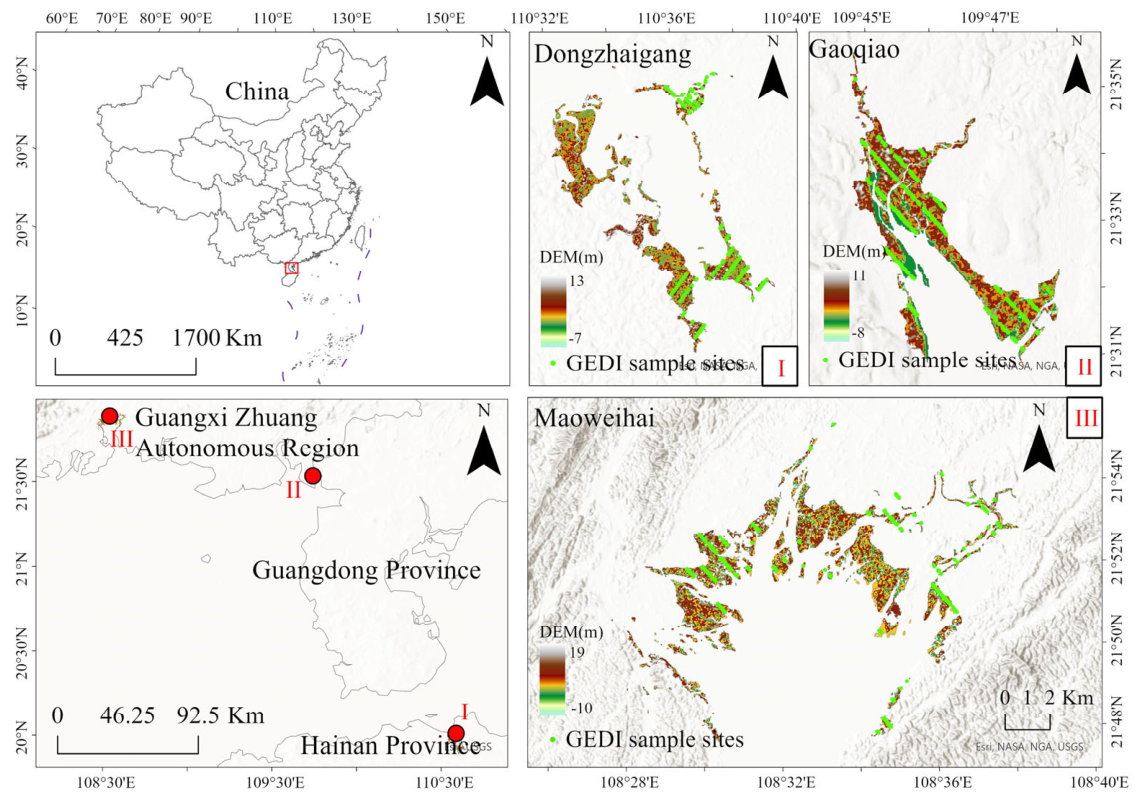
Three representative mangrove ecosystems along the South China coast were selected to evaluate the applicability of GEDI, Sentinel-1, and Sentinel-2 MCH retrieval under contrasting structural and hydrological settings: Dongzhaigang (DZG) in Hainan Province (19°51′–20°01′N, 110°30′–110°37′E), Gaoqiao (GQ) in Guangdong Province (21°30′–21°35′N, 109°40′–109°50′E), and Maoweihai (MWH) in Guangxi Province (21°42′–21°55′N, 108°25′–108°40′E) (Figure 1). Spanning a tropical-to-subtropical monsoonal gradient with distinct structural and hydrological characteristics, these sites have been frequently utilized in national and regional mangrove remote-sensing studies [10]. Furthermore, they represent a gradient from mature, closed-canopy mangrove stands to fragmented estuarine mangrove mosaics, thereby providing a suitable testbed for assessing whether kernel-based spectral features can improve MCH retrieval under varying canopy-density and background-complexity conditions [15,27,28].

DZG is a ria-type bay featuring a tropical monsoon climate and mixed semidiurnal tides. Characterized by multi-layered, closed canopies of Rhizophora stylosa exceeding 10 m, its closed and multi-layered structure creates a high-biomass setting where conventional optical vegetation indices are more prone to spectral saturation [28]. GQ represents one of the most extensive contiguous subtropical mangrove forests in mainland China, governed by irregular diurnal tides (with a range of 2.0 m), making it ideal for evaluating prediction stability under continuous forest cover combined with heterogeneous hydrological backgrounds [29].

In contrast, MWH is a semi-enclosed estuarine system subject to significant riverine discharge and high precipitation (>2100 mm). Notably, it experiences regular diurnal tides with a large mean range (2.24–2.5 m), leading to frequent tidal inundation. Mangroves in this area, primarily Avicennia marina, exist as fragmented mosaic patches [30]. Consequently, this site was selected to test model robustness under pronounced mixed-pixel and landscape-fragmentation effects.

2.2. Overall Workflow

The methodological workflow comprised five sequential steps. First, GEDI L2A waveform metrics were filtered and utilized as footprint-level reference samples for MCH. Second, Sentinel-2 Level-2A surface reflectance images and Sentinel-1 C-band SAR backscatter data were composited during site-specific growing seasons to generate spatially continuous optical-radar predictors. Third, traditional vegetation and water-related indices were calculated and transformed into their kernel-based counterparts, yielding three distinct feature configurations: traditional indices, kernel-based indices, and fused indices [16,31,32,33]. Fourth, four regression models—Random Forest (RF), XGBoost, 1D-Convolutional Neural Network (1D-CNN), and DeepForest—were trained and compared under identical feature configurations [22,24,34]. Finally, model performance was evaluated using repeated train–test splits, and spatially continuous maps of MCH and ensemble dispersion were generated across the three study areas.

This workflow was structured to address the three primary objectives of this study: comparing the sensitivity and saturation characteristics of traditional versus kernel-based indices, evaluating model performance across different feature configurations, and assessing the spatial applicability of the optimized retrieval framework over contrasting mangrove landscapes.

2.2.1. GEDI-Derived Canopy Height Samples

To achieve high-precision MCH inversion, this study utilized spaceborne LiDAR observations from the GEDI mission as reliable footprint-level reference samples for canopy height [35].

GEDI Level-2A Version 2 (v002) data were employed as footprint-level reference observations for MCH. GEDI (https://gedi.umd.edu/ (accessed on 18 July 2026)) is a spaceborne full-waveform LiDAR mission designed to characterize vegetation vertical structure, canopy height, terrain elevation, and biomass-related metrics by sampling the Earth’s surface from the International Space Station [11]. Compared to the v001 product, the v002 product significantly optimizes denoising algorithms and waveform fitting accuracy across diverse vegetation types. GEDI data comprises multiple observation tracks containing full-power beams (e.g., BEAM0101, BEAM0110, BEAM1000, BEAM1011) and coverage beams (e.g., BEAM0000, BEAM0001). Strong beams possess higher signal-to-noise ratios (SNRs) and ensure superior stability in canopy height retrieval. To guarantee laser penetration and vertical structural accuracy, footprints with a sensitivity threshold below 0.9 (90%) were filtered out.

The relative height metric $rh98$, defined as the height below which 98% of the cumulative waveform energy is returned, was selected as the proxy for MCH because it approximates upper canopy height while remaining less sensitive to waveform noise than $rh100$. Footprints were filtered using standard quality layers, retaining only those meeting $\mathrm{quality}\text{\_}\mathrm{flag}=1$ and $\mathrm{degrade}\text{\_}\mathrm{flag}=0$ to eliminate low-quality waveforms, poor geolocation, or cloud contamination.

To ensure temporal consistency between spaceborne LiDAR observations and multi-source optical/SAR predictors, the temporal window for GEDI footprints and optical/SAR imagery was strictly synchronized within each respective study site according to data availability: from 1 May 2022, to 31 October 2022, for Gaoqiao; from 1 April 2022, to 31 October 2022, for Maoweihai; and from 1 April 2023, to 31 July 2025, for Dongzhaigang. Cloud-filtered Sentinel-2 observations and Sentinel-1 SAR data during these corresponding site-specific windows were processed into median composites to mitigate short-term meteorological fluctuations and tidal extremes. Specifically, to extract predictor values for each GEDI footprint, a footprint rasterization and co-registration workflow was implemented within Google Earth Engine (GEE): GEDI footprint locations were rasterized onto the 10 m spatial grid of the Sentinel imagery, allowing direct pixel-level spatial stacking and extraction while ensuring computational efficiency and precise co-registration. Furthermore, for the Dongzhaigang (DZG) site, which required an extended temporal span (2023–2025) due to persistent cloud cover, a multi-year median compositing strategy combined with C-band SAR integration was adopted to ensure adequate footprint density. This long-term temporal aggregation effectively smoothed out inter-annual phenological shifts and localized short-term growth dynamics, maintaining robust temporal consistency between the optical-radar predictors and the GEDI reference samples.

To address potential tidal interferences in intertidal mangrove environments—such as inundation effects reducing reflectance via water absorption or soil moisture variations—long-term median compositing and multi-source feature stacking (incorporating Sentinel-1 SAR features insensitive to water inundation) were jointly employed [36]. Furthermore, rigorous spatial filtering was applied: footprints located on slopes greater than ${30}^{\circ }$ (derived from SRTM DEM) were excluded to prevent footprint smearing and terrain-induced height distortions [37]. A conservative NDVI threshold of $>0.05$ was intentionally enforced to exclude pure water bodies and deep-sea surfaces while safely preserving highly stressed, sparse, or low-stature mangrove pixels (such as stunted dwarf stands whose greenness often approaches bare-soil baselines). While this low threshold risks minor commission errors over high-turbidity tidal flats or wet sediments, such edge-pixel ambiguities were effectively constrained by intersecting footprints strictly with a high-accuracy baseline mangrove mask. Finally, only footprints falling within the site-specific baseline mangrove mask (derived from high-resolution imagery and Global Mangrove Watch products with an overall accuracy $>90\%$) were retained.

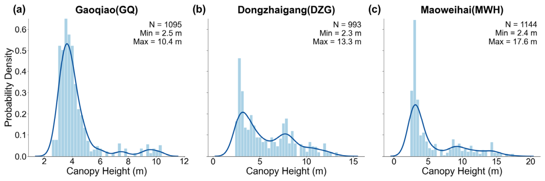
The MCH samples across the three study sites exhibited distinct structural heterogeneity (Figure 2). Gaoqiao (GQ) is characterized by a 3–4 m unimodal distribution ($N=1095$; range: 2.5–10.4 m), whereas Dongzhaigang (DZG) displays a broader, bimodal profile ($N=993$; 2.3–13.3 m). In contrast, Maoweihai (MWH) presents a right-skewed distribution with a sharp peak at 3 m and a long tail extending to 17.6 m ($N=1144$; 2.4–17.6 m). These structural variations reflect the diverse successional stages of the mangrove stands, providing a robust, comprehensive gradient for model training and cross-site generalizability.

2.2.2. Sentinel-1 and Sentinel-2 Compositing and Predictors

Sentinel-2 multispectral imagery, featuring high spatial resolution (10 m for visible and near-infrared bands) and frequent revisit capability, combined with Sentinel-1 C-band synthetic aperture radar (SAR) data, provides an advanced optical-radar synergistic backbone for characterizing regional mangrove biophysical parameters [38]. In this study, Sentinel-2 Level-2A bottom-of-atmosphere (BOA) surface reflectance products and Sentinel-1 Ground Range Detected (GRD) high-resolution backscatter data were utilized. Sentinel-2’s surface reflectance represents the fraction of incoming solar radiation reflected from the Earth’s surface after atmospheric correction, whereas Sentinel-1 provides backscatter coefficients (${\sigma }^{\circ }$) in VV and VH polarizations, which are highly sensitive to canopy structure, surface roughness, and moisture conditions independently of cloud cover.

All Sentinel-1 and Sentinel-2 preprocessing tasks were conducted within Google Earth Engine (GEE), a cloud-based platform designed for large-scale geospatial data processing. To maintain strict temporal consistency with the GEDI reference observations, imagery was selected and aggregated within the corresponding site-specific growing-season windows defined previously.

A streamlined image synthesis workflow was implemented to ensure the fidelity of the spectral and radar composites. For Sentinel-2, initial filtering excluded granules with cloud cover exceeding 15% based on metadata. Subsequently, residual clouds and cirrus shadows were masked using the QA60 quality assessment band. A median compositing technique was then applied to the cloud-masked Sentinel-2 observations to generate a seamless, representative optical image for each site. For Sentinel-1, GRD data were preprocessed in GEE through thermal noise removal, radiometric calibration, and terrain correction using the SRTM DEM to derive normalized backscatter coefficients in VV and VH polarizations, followed by temporal median compositing matching the site-specific optical windows. This multi-sensor optical-SAR integration approach is particularly effective in mangrove studies because it suppresses transient noise, outliers, and ephemeral tidal inundation effects, thereby providing a standardized representation of the mangrove ecosystem [35]. Crucially, all subsequent feature extraction, spatial modeling, and accuracy assessments were comprehensively executed based on this standardized Sentinel-1 and Sentinel-2 dataset.

2.3. Feature Engineering and Characterization

2.3.1. Traditional Vegetation and Water-Related Indices

To establish a multidimensional feature space and provide a comparative baseline for advanced modeling architectures, a set of traditional remote sensing indices was systematically calculated from Sentinel-2 surface reflectance and Sentinel-1 backscatter data to characterize complementary spectral and structural dimensions relevant to mangrove canopy and background conditions. Specifically, core optical vegetation and canopy structure indices—including NDVI, EVI, VARI, and SLAVI—were derived from Sentinel-2 to represent canopy vigor, vegetation fraction, and structural variations. To capture subtle color variations and pigment dynamics, specialized indicators such as SIPI and ExGR were incorporated. Furthermore, water- and soil-background adjustment features, including MNDWI, AWEInsh, and BSI, were utilized to mitigate the confounding influence of exposed intertidal sediments, mixed vegetation-soil pixels, and tidal inundation dynamics. Finally, cross-domain microwave radar metrics, represented by the Sentinel-1 dual-polarization radar vegetation index (S1_DpRVI), were integrated at the feature level to capture backscatter intensity effects that are particularly crucial in complex mangrove estuarine environments [38].

2.3.2. Construction of Kernel-Based Indices

Kernel-based indices were constructed to extend traditional spectral-index formulations into a non-linear feature space, aiming to mitigate the asymptotic saturation commonly encountered in high-biomass mangrove canopies [20]. For any two spectral or composite variables $V_1$ and $V_2$, the non-linear relationship was captured using the Gaussian Radial Basis Function (RBF) kernel similarity:

$$K\left(V_1,V_2\right)=exp\left(-{\displaystyle \frac{(V_1-V_2{)}^2}{2{\sigma }^2}}\right)$$

(1)

where $\mathsf{\sigma }$ is the kernel scale parameter controlling the degree of nonlinear transformation. A small $\mathsf{\sigma }$ increases sensitivity to subtle spectral differences but may amplify noise, whereas a large $\mathsf{\sigma }$ smooths the feature space and may weaken discrimination among dense-canopy pixels.

For normalized-difference-type indices, kernelization was implemented by replacing the original linear band contrast with a kernel similarity term. For example, the kernelized normalized-difference formulation can be written as:

$$kNDVI=1-exp\left(-{\displaystyle \frac{(NIR-Red{)}^2}{2{\sigma }_{NIR,Red}^2}}\right)$$

(2)

where the adaptive scale parameter ${\sigma }_{NIR,Red}$ is parameterized locally by the meaning of the two interacting bands. The Gaussian kernel therefore transforms the original spectral contrast into a bounded non-linear response.

Following this RBF projection framework, ten traditional vegetation, water, soil, and radar indices were extended into their kernel-based counterparts (

Table 1. Summary of traditional and kernel-based vegetation indices used in this study.

Full Name	Original Formulation	Kernelized Formulation	Ref.
Kernel Normalized Difference Vegetation Index	NDVI = ${\displaystyle \frac{\mathrm{N}\mathrm{I}\mathrm{R}-\mathrm{R}\mathrm{e}\mathrm{d}}{\mathrm{N}\mathrm{I}\mathrm{R}+\mathrm{R}\mathrm{e}\mathrm{d}}}$	$kNDVI=1-\exp \left(-{\displaystyle \frac{{\left(NIR-Red\right)}^2}{2{\sigma }_{NIR,Red}^2}}\right)$	[20]
Kernel Enhanced Vegetation Index	$\mathrm{EVI}=G\times {\displaystyle \frac{\mathrm{NIR}-\mathrm{Red}}{\mathrm{NIR}+C_1\times \mathrm{Red}-C_2\times \mathrm{Blue}+L}}$	$k\mathrm{EVI}=G\times {\displaystyle \frac{k\left(\mathrm{NIR},\mathrm{NIR}\right)-k\left(\mathrm{NIR},\mathrm{Red}\right)}{k\left(\mathrm{NIR},\mathrm{NIR}\right)+C_1\times k\left(\mathrm{Red},\mathrm{Red}\right)-C_2\times k\left(\mathrm{Blue},\mathrm{Blue}\right)+L}}$	[20,39]
Kernel Modified Normalized Difference Water Index	$\mathrm{M}\mathrm{N}\mathrm{D}\mathrm{W}\mathrm{I}={\displaystyle \frac{\mathrm{G}\mathrm{r}\mathrm{e}\mathrm{e}\mathrm{n}-\mathrm{S}\mathrm{W}\mathrm{I}\mathrm{R}}{\mathrm{G}\mathrm{r}\mathrm{e}\mathrm{e}\mathrm{n}+\mathrm{S}\mathrm{W}\mathrm{I}\mathrm{R}}}$	$kMNDWI=1-\exp \left(-{\displaystyle \frac{{\left(Green-SWI{R}_1\right)}^2}{2{\sigma }_{Green,SWI{R}_1}^2}}\right)$	[20,40]
Kernel Automated Water Extraction Index	$\mathrm{AWEInsh}=4\times \left(\mathrm{Green}-\mathrm{SWIR}1\right)-\left(0.25\times \mathrm{NIR}+2.75\times \mathrm{SWIR}2\right)$	$kAWEInsh=\exp \left(-{\displaystyle \frac{1}{2{\sigma }_{\mathrm{AWEI}}^2}}{\left(\mathrm{Blu}+2.5\times \mathrm{Green}-1.5\times \mathrm{NIR}-1.5\times {\mathrm{SWIR}}_1-0.25\times {\mathrm{SWIR}}_2\right)}^2\right)$	[16,20]
Kernel Visible Atmospherically Resistant Index	$VARI={\displaystyle \frac{Green-Red}{Green+Red-Blue}}$	$kVARI=\exp \left(-{\displaystyle \frac{{\left(Green-Red\right)}^2}{2{\sigma }^2}}\right)\times {\displaystyle \frac{Green}{Green+Red-Blue}}$	[20,41]
Kernel Soil-Adjusted Index	$BSI={\displaystyle \frac{({SWIR}_1+Red)-(NIR+Blue)}{({SWIR}_1+Red)+(NIR+Blue)}}$	$kBSI=\exp \left(-{\displaystyle \frac{{\left(\left(SWI{R}_1+Red\right)-\left(NIR+Blue\right)\right)}^2}{2{\sigma }^2}}\right)$	[20,42]
Kernel Structure Sensitive Pigment Index	$SIPI={\displaystyle \frac{NIR-Blue}{NIR+Red}}$	$kSIPI={\displaystyle \frac{1-\exp \left(-\frac{{\left(NIR-Blue\right)}^2}{2{\sigma }_{NIR,Blue}^2}\right)}{1-\exp \left(-\frac{{\left(NIR-Red\right)}^2}{2{\sigma }_{NIR,Red}^2}\right)}}$	[20,43]
Kernel Specific Leaf Area Vegetation Index	$SLAVI={\displaystyle \frac{NIR}{Red+{SWIR}_2}}$	$kSLAVI=\exp \left(-{\displaystyle \frac{{\left(NIR-\left(Red+SWIR\right)\right)}^2}{2{\sigma }^2}}\right)$	[20,44]
Kernelized Excess Green Index	$ExGR=2Green-Red-Blue$	$kExG=\exp \left(-{\displaystyle \frac{{\left(2\times Green-Red-Blue\right)}^2}{2{\sigma }^2}}\right)$	[20,45]
Kernel Sentinel-1 Dual-Polarization Radar Vegetation Index	$DpRVI={\displaystyle \frac{4V{H}_{pow}}{V{V}_{pow}+V{H}_{pow}}}$	$kDpRVI=4\times {\displaystyle \frac{\exp \left(-\frac{V{H}_{pow}^2}{2{\sigma }^2}\right)\times V{H}_{pow}}{V{V}_{pow}+V{H}_{pow}}}$	[20,46]

). It should be explicitly noted that certain formulations incorporate self-similarity terms (e.g., $k\left(V_1,V_1\right)$). Given that the RBF kernel evaluates self-similarity to a constant of unity ($K\left(x,x\right)=1$), these terms act as bounded normalization anchors rather than preserving the exact proportional responses of original linear ratios; thus, physical properties of conventional indices are not automatically retained. To clarify, while certain established formulations (e.g., $kNDVI$) are grounded in theoretical kernel derivations, other variants implemented here represent exploratory non-linear feature transformations tailored for high-biomass structural mapping. It is important to emphasize that these kernel-based indices were not presupposed to universally outperform traditional linear formulations. Rather, they were implemented here as an exploratory framework to rigorously evaluate their true generalization capacity, saturation thresholds, and noise-suppression boundaries under multi-model architectures across contrasting mangrove environments.

2.3.3. Parameter Optimization and Robustness

Notably, the configuration of the scale parameter ($\sigma$) within the kernel function is pivotal to the model’s local sensitivity and feature representation. Rather than relying on a global static constant or an ad hoc site-specific parameter, $\sigma$ was formulated as an index-specific and spatially adaptive parameter, analytically derived from the local statistics of the interacting spectral or radar bands corresponding to each kernelized index. Specifically, for each individual index, $\sigma$ was adaptively parameterized using the local mean or composite variance within a moving window. To strictly exclude potential information leakage and ensure reproducibility, this local parameter estimation was performed independently within each training fold during cross-validation, using exclusively the training data partitions rather than the global dataset or validation folds. This index-specific local adaptive formulation ensures that the kernel function dynamically accommodates the distinct radiometric properties and spectral dynamic ranges of different VIs.

2.3.4. Feature Collinearity and Redundancy Diagnostics

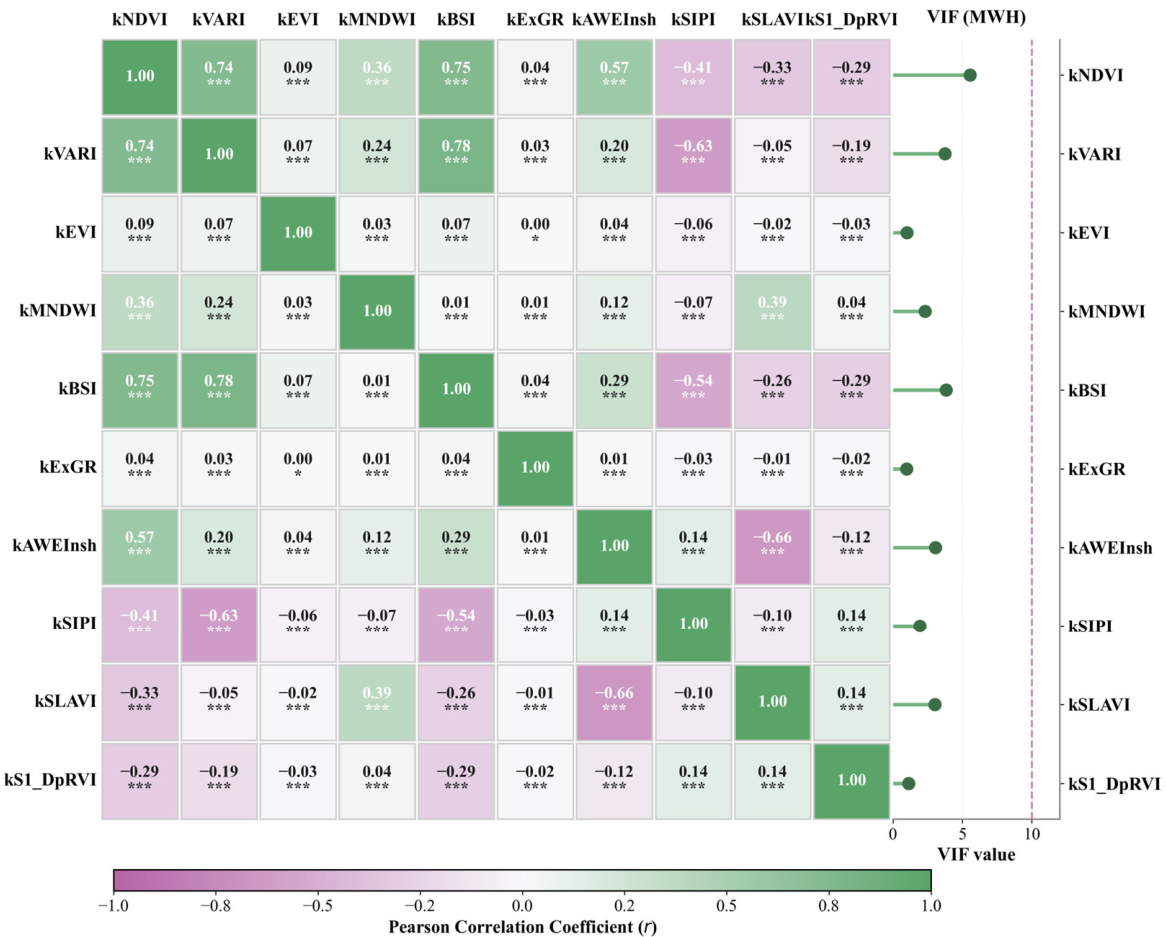
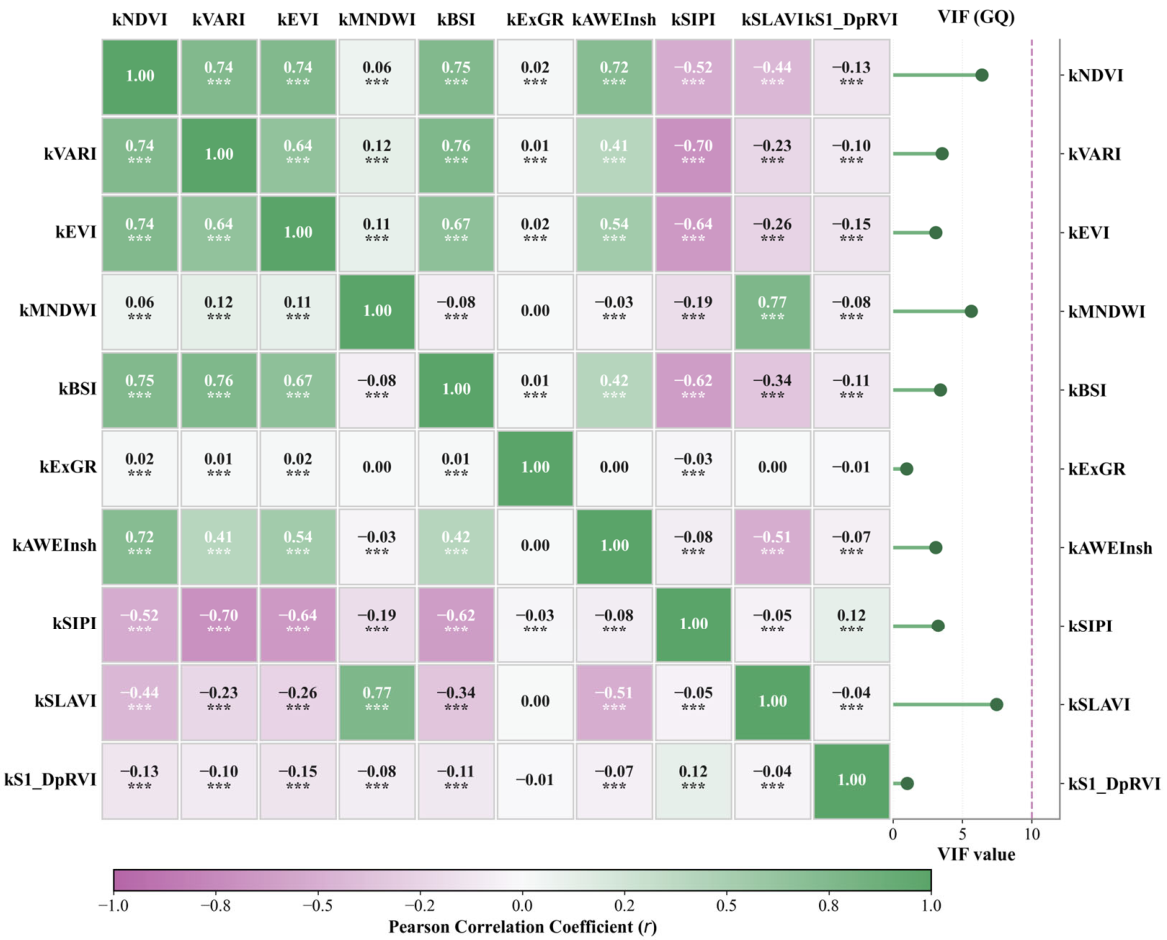
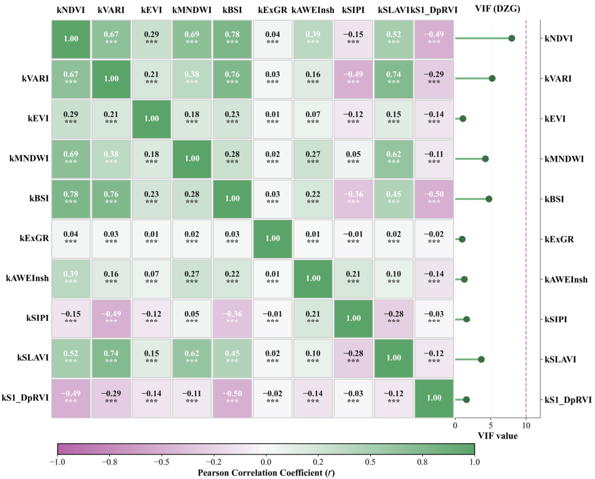
To address potential concerns regarding feature redundancy and multicollinearity among the derived kernel-based indices, a rigorous diagnostic framework utilizing the Pearson correlation matrix and Variance Inflation Factor (VIF) was implemented across all study zones. Although kernel transformations project spectral indices into a non-linear feature space, localized high pairwise correlations (e.g., $r=0.78$ between $\mathrm{kNDVI}$ and $\mathrm{kBSI}$, or $r=0.77$ between $\mathrm{kMNDWI}$ and $\mathrm{kSLAVI}$ in specific zones) can occasionally emerge.

However, comprehensive VIF diagnostics explicitly confirm that all feature VIF values remain well below the conventional critical threshold of 10.0 (with maximum VIF values restricted under 7.5 across all regions) [47]. This indicates that despite moderate-to-high pairwise collinearity among certain kernel features, the non-linear expansion does not lead to severe multicollinearity or structural matrix instability. Consequently, the combined feature set effectively retains non-redundant variational information suitable for robust machine learning assimilation, as illustrated in the regional correlation and VIF profiles (Figure 3, Figure 4 and Figure 5).

2.4. Predictive Modeling Framework

2.4.1. Algorithmic Implementation and Cross-Validation

Following the regional feature diagnostics across all study zones (Figure 3, Figure 4 and Figure 5), to guarantee a robust and unbiased comparative analysis across different levels of model complexity, all predictive architectures were systematically trained and validated under identical sample conditions. To mitigate the inflation of accuracy metrics caused by spatial autocorrelation among adjacent GEDI footprints, a spatially blocked cross-validation scheme (with a spatial block size of 2 km $\times$ 2 km, designed to exceed the local range of residual spatial autocorrelation) was integrated into the training pipeline, ensuring complete spatial separation between training and evaluation folds.

For each modeling scenario, the independent variables corresponding to the multi-feature configurations were linked against footprint-level GEDI LiDAR references. A nested cross-validation design was implemented to strictly decouple hyperparameter optimization from final performance evaluation, thereby preventing information leakage. Specifically, a 5-fold outer spatial block validation and a 3-fold inner spatial block cross-validation loop were established. To prevent cross-track contamination, adjacent GEDI footprints belonging to the same orbital overpass within the same spatial block were assigned exclusively to the same fold. Hyperparameter tuning was conducted within this inner loop powered by randomized grid searches and Bayesian optimization (implemented in Python 3.9), with distinct random seeds assigned to each individual model to ensure independent stochastic initialization. Crucially, to ensure a completely fair comparison, identical spatial block partitions were strictly maintained across all candidate regression models and feature configurations. Furthermore, to eliminate any potential data leakage during preprocessing, all data scaling and normalization parameters were estimated exclusively from the training folds and subsequently applied to the corresponding validation and testing folds.

2.4.2. Regression Models for MCH Retrieval

Four regression models were employed to retrieve mangrove canopy height (MCH) using Sentinel-1 and Sentinel-2 feature sets: Random Forest (RF), XGBoost, 1D-CNN, and DeepForest [22,24,34,48]. The models represented different levels of algorithmic complexity, from conventional tree ensembles to gradient boosting, neural-network-based feature extraction, and tree-based deep ensemble learning. The detailed search spaces and optimized hyperparameters for all models are summarized in

Table 2. Search spaces and optimized hyperparameters for the four regression models in mangrove canopy height estimation.

Model	Parameter	Search Space	Optimal Value
RF	n_estimators	{100, 200, 300, 500}	500
	max_features	{‘sqrt’, ‘log2’, 0.5, 0.8}	‘sqrt’
	max_depth	{10, 20, 30, None}	None
XGBoost	n_estimators	{100, 300, 500, 1000}	500
	learning_rate	[0.01, 0.2]	0.05
	max_depth	[3, 9]	6
	subsample	[0.5, 1.0]	0.8
	colsample_bytree	[0.5, 1.0]	0.8
1D-CNN	learning_rate	{${10}^{-4}$, ${10}^{-3}$, ${10}^{-2}$}	${10}^{-3}$
	batch_size	{32, 64, 128}	64
	dropout	[0.3, 0.4]	0.3
DeepForest	n_trees_per_forest	Fixed	500
	max_cascade_layers	[2, 10]	6 (Early stopped)
	max_depth_per_tree	Fixed	16

.

RF served as a robust ensemble baseline. It constructs multiple decision trees using bootstrap samples and random feature subsets, and predictions are obtained by averaging individual tree outputs. This structure handles nonlinear relationships, high-dimensional predictors, and multicollinearity. In this study, RF was trained under all feature configurations. Key hyperparameters, including the number of trees ($n_{\mathrm{estimators}}=500$, searched within $\left[100,1000\right]$), maximum features per split ($max\_features=\text{‘}\mathrm{sqrt}\text{’}$), maximum tree depth ($max\_depth=16$, searched within $\left[4,30\right]$), and minimum samples per leaf, were optimized by the inner spatial block cross-validation.

XGBoost was included as a gradient-boosting benchmark. Unlike RF, which builds trees in parallel, XGBoost sequentially adds trees to reduce residual errors from previous iterations and incorporates regularization terms to control model complexity. XGBoost also includes sparsity-aware learning and efficient tree construction. The optimized XGBoost model was trained for each feature configuration. Hyperparameters, including the number of boosting rounds ($400$), learning rate ($0.01$, searched within $\left[0.001,0.1\right]$), maximum tree depth ($5$, searched within $\left[3,10\right]$), subsampling ratio ($0.85$), column-sampling ratio ($0.85$), and L1/L2 regularization parameters, were systematically optimized through the nested spatial cross-validated grid search.

A 1D-CNN was implemented to examine whether local feature extraction along multi-source spectral-index sequences could enhance MCH retrieval. The input vector consisted of structured sequences of engineered feature indices for each configuration. To mitigate potential sensitivity to feature ordering, alternative randomized sequence permutations were evaluated to ensure robustness. The network architecture comprised one-dimensional convolutional layers, activation functions, pooling operations, dropout regularization, and fully connected regression layers. Because 1D-CNN performance can be sensitive to sample size, feature ordering, and hyperparameter settings, it was treated as a comparative baseline rather than a presumed superior model, given that GEDI-derived training samples are footprint-based and inherently more limited than the large datasets typically required by deep neural networks [13]. By traversing these input sequences of multi-source kernelized vegetation indices with 1D kernels, the model captured latent spectral–structural interactions among adjacent indices, distilling high-level representations closely coupled with mangrove canopy vertical complexity rather than raw spectral bands. The optimized 1D-CNN regressor adopted a deep cascaded structure consisting of multiple convolutional layers followed by dense layers. To facilitate gradient propagation and accelerate convergence, each convolutional layer was integrated with a batch normalization layer and a Leaky ReLU activation function. Dimensionality reduction and feature refinement were performed via max-pooling ($MaxPooling1D$). Training was governed by the Adam optimizer ($\mathrm{learning}\mathrm{rate}=0.0005$, $\mathrm{clipnorm}=0.5$, $\mathrm{batch}\mathrm{size}=32$) over a maximum of 300 epochs, utilizing early stopping ($\mathrm{patience}=30$ on validation loss) and learning rate reduction ($\mathrm{factor}=0.5$). A global average pooling layer summarized feature maps while preserving the semantic integrity of the spectral–structural sequence. The final regression head consisted of a dense layer with dropout regularization ($0.3\text{–}0.4$) to mitigate overfitting and enforce a physical constraint bounding predictions within valid mangrove height limits across the heterogeneous landscapes of MWH, GQ, and DZG [19].

DeepForest (also known as gcForest) was utilized as a tree-based deep ensemble model. Unlike conventional neural networks, gcForest constructs a multi-layer cascade of tree ensembles and performs layer-wise feature transformation without backpropagation. It serves as an alternative deep learning framework featuring fewer hyperparameters and stronger applicability to moderate-sized tabular datasets. The architecture incorporates two core mechanisms: multi-grained scanning, which uses sliding windows of varying dimensions to traverse input feature sequences and capture multi-scale contextual interactions (analogous to receptive fields in CNNs); and a cascade forest, which channels extracted feature vectors into a multi-level structure comprising random forests and completely random trees (each forest containing 500 trees with a maximum depth of 16). Each cascade level receives augmented feature vectors from the previous layer, enabling iterative feature refinement and progressive noise reduction to isolate structural components indicative of MCH. Governed by the nested spatial validation architecture, critical hyperparameters—including maximum cascade depth (dynamically capped at up to 10 layers via an automated early stopping rule that halts growth if validation performance fails to improve across consecutive layers) and feature subsampling ($max\_features=0.8$)—were optimized using Bayesian optimization [49,50].

2.5. Model Validation and Accuracy Assessment

To rigorously evaluate the predictive accuracy and spatial generalization proficiency of the regression models, an independent spatial block validation framework was implemented. Consistent with the nested cross-validation design described in Section 2.4.1, the GEDI footprint dataset within each study site was partitioned into spatially distinct training and testing subsets using block-based partitioning. This spatial partitioning ensures that the testing phase remains geographically separated from the training data, thereby mitigating the inflation of performance metrics typically induced by spatial autocorrelation and providing an unbiased assessment of the model’s ability to predict canopy height in geographically adjacent yet unobserved plots [51]. Model performance was evaluated using the coefficient of determination ($R^2$), root mean square error (RMSE) and mean absolute error (MAE).

To further characterize the robustness and stability of the inversion framework, especially when dealing with the stochastic nature of machine learning algorithms, each model was subjected to 50 independent Monte Carlo-style iterations with randomized spatial block splits. We subsequently analyzed the statistical distribution of these metrics through histograms and boxplots, which allowed for the comprehensive quantification of model prediction variability [42].

To rigorously evaluate the performance enhancements achieved by the hybrid feature space, a paired Wilcoxon signed-rank test was conducted to examine the statistical significance of performance differences between the single-feature baselines and the combined feature configuration. Given the non-normal distribution of multi-round evaluation metrics across localized ecosystems, the paired structure was established by aligning the evaluation scores ($R^2$, RMSE, and MAE) derived from the exact same spatial validation folds. The null hypothesis assumed no median difference between paired feature strategies, with the significance thresholds strictly set at $p<0.05$ and $p<0.01$.

After model training and cross-validation, the optimized model–feature combinations were applied to the multi-source composite predictors to generate spatially continuous MCH maps for DZG, GQ, and MWH. Predictions were restricted to mangrove pixels using the mangrove mask to avoid extrapolation into non-mangrove surfaces.

Ensemble prediction dispersion was quantified using the standard deviation of pixel-level predictions across the 50 repeated runs [52]:

$$S{D}_{pred}=\sqrt{{\displaystyle \frac{1}{m-1}}{\displaystyle \sum _{j=1}^m}{\left({\hat{y}}_j-{\hat{y}}_{mean}\right)}^2}$$

(3)

where ${\hat{y}}_j$ is the predicted MCH for a pixel in the $j$-th repeated run, $\overline{y}$ is the mean prediction across repeated runs, and $m=50$. The resulting dispersion maps were used to identify spatial regions susceptible to prediction instability, such as forest–water boundaries, fragmented patches, and dense stands affected by optical saturation.

Spatial maps were interpreted together with model accuracy metrics. This joint evaluation was necessary because the objective of MCH mapping was not only to maximize footprint-level prediction accuracy but also to produce spatially coherent and reliable canopy-height surfaces, while recognizing that lower prediction dispersion achieved by tree-based deep ensembles reflects enhanced stability rather than the complete elimination of estimation error.

3. Results

3.1. Correlation-Based Sensitivity of Spectral Indices to Mangrove Canopy Height

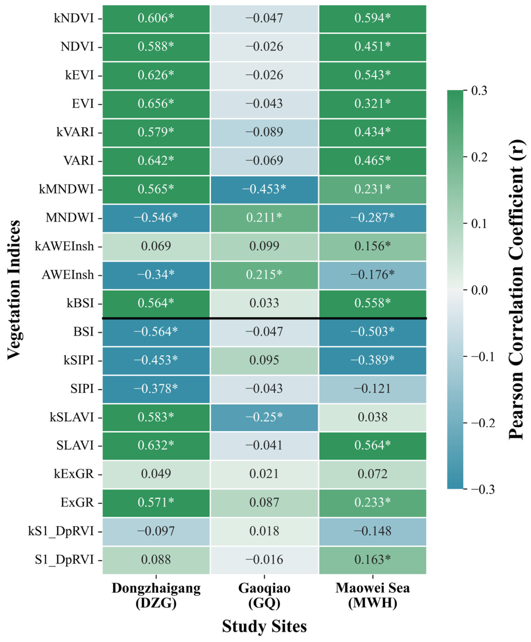
To evaluate the spectral sensitivity of different feature groups to GEDI-derived MCH, Pearson correlation coefficients between each remote sensing index and GEDI $rh98$ were calculated across the three study sites (Figure 6). Unlike the weak associations observed in preliminary assessments, the updated multi-source feature sets revealed substantially enhanced correlation magnitudes, with maximum absolute $r$ values reaching up to $0.656$ in DZG, $0.453$ in GQ, and $0.564$ in MWH.

A notable pattern in Figure 6 is the cross-site consistency observed among core vegetation indices. Rather than complete sign inversions across all indices, conventional and kernel-based vegetation indices such as $\mathrm{kNDVI}$, $\mathrm{NDVI}$, $\mathrm{kEVI}$, $\mathrm{EVI}$, $\mathrm{kVARI}$, and $\mathrm{VARI}$ maintained consistent positive correlations with MCH across both DZG and MWH (with $r$ values ranging from $0.321$ to $0.656$, all $p<0.05$). This structural alignment confirms that robust greenness and structural indices reliably capture canopy height variations in well-developed mangrove ecosystems where canopy closure is pronounced [17].

However, pronounced spatial heterogeneity and sign inversions persisted in specific environments, particularly among water/moisture-related indices. For instance, indices such as $\mathrm{MNDWI}$ and $\mathrm{AWEInsh}$ exhibited positive correlations in GQ ($r=0.211$ and $0.215$, respectively) but shifted to significant negative correlations in DZG ($r=-0.546$ and $-0.34$) and MWH ($r=-0.287$ and $-0.176$, respectively). Similarly, overall correlation magnitudes at the GQ site remained generally subdued and statistically insignificant for most indices, with the exception of $\mathrm{kMNDWI}$ ($r=-0.453$) and $\mathrm{kSLAVI}$ ($r=-0.25$).

This regional divergence and sign reversal stems from distinct hydrodynamic regimes and site-specific tidal inundation frequencies. In Gaoqiao (GQ), which predominantly occupies higher intertidal positions or micro-topographic edges with moderate moisture, higher water-index values often trace moist, nutrient-rich estuarine margins that favor mangrove development, resulting in a positive association. Conversely, in Dongzhaigang (DZG) and Maoweihai (MWH)—both characterized by extensive tidal networks and frequent inundation—high water-index values directly capture deep water columns, saturated muddy substrates, or prolonged tidal submersion. In these low-intertidal zones, severe hydrodynamic stress and water absorption suppress canopy growth, creating an inverse relationship where elevated water indices correspond to lower, water-stressed, or sparse mangrove stands. Furthermore, the localized saturation limits of traditional indices across varying structural stages underscore the necessity of employing multi-source composite features and advanced machine learning models rather than relying on single linear indices for universal MCH retrieval.

3.2. Spectral Value Redistribution and Its Implication for Saturation Expression

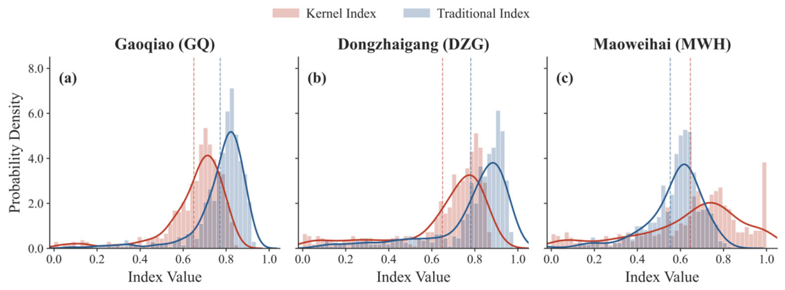
To systematically elucidate the non-linear scaling behaviors and spectral redistribution mechanisms of the constructed spectral features, the probability density distributions (PDDs) of traditional NDVI and the proposed kNDVI were comparatively evaluated across the three distinct mangrove ecosystems (Figure 7). Characteristically, the traditional linear NDVI consistently exhibited a compressed, leptokurtic distribution with a prominently sharp peak across the sites, indicating that a substantial proportion of mangrove pixels were constrained within narrow greenness intervals due to linear vector-space limitations.

To ensure rigorous cross-index mathematical compatibility and statistical alignment within the unified [0, 1] operational domain, a standard local linear scaling operator was executed to map the kernelized descriptors, with scaling limits determined strictly based on training datasets to prevent data leakage. Specifically, within the mature and dense forest communities of Gaoqiao (GQ, Figure 7a), the traditional NDVI exhibited a high-value clustering, signifying an asymptotic upper-bound compression effect as the index approached its intrinsic saturation plateau under high-canopy-closure conditions. Conversely, the proposed kNDVI shifted the distribution median downward while broadening the distribution spread. This downward shift does not imply a direct recovery of lost structural information; rather, it indicates that the densely clustered high values originally squeezed within the upper saturation zone were redistributed toward a broader numerical range, thereby revising feature representation under high biomass conditions and widening the spatial dynamic range. This structural dispersion suggests that the Gaussian kernel mechanism effectively redistributes the high-value spectrum, converting compressed vegetative plateaus into a more widely spread value continuum.

Within the mature, closed, and multi-layered canopy environments of Dongzhaigang (DZG, Figure 7b), the traditional NDVI peaked sharply at a high level, reflecting strong susceptibility to signal compression in dense canopy patches. In contrast, the scale-normalized kNDVI shifted downward with an enhanced spread across lower-to-moderate value ranges. By dispersing the clustered high values into a non-linear numerical continuum, this downward adjustment relieves feature compression near the upper boundary. This prominent broadening of the PDD curve demonstrates that the kernelized formulation effectively stretches restricted dynamic ranges.

Similarly, within the fragmented estuarine habitats of Maoweihai (MWH, Figure 7c), the traditional NDVI stabilized at a high clustering level, whereas the kNDVI adjusted smoothly to a lower median trajectory. This balanced alignment confirms that the kernel-transformed trajectory maintains structural stability, effectively buffering against saturation effects in dense core zones while preserving sensitivity in background-dominated landscapes. Cumulatively, these cross-site empirical distributions indicate that the proposed kernelized framework smoothly modulates feature distribution skewness while maintaining baseline spectral performance across varying ecological gradients.

3.3. Prediction Performance of Model Architecture and Feature Configuration in Different Locations

3.3.1. Quantitative Benchmarking of Model Architecture

To rigorously evaluate the predictive capabilities of different algorithmic paradigms, four representative machine learning and deep learning architectures—DeepForest, XGBoost, Random Forest (RF), and 1D-CNN—were benchmarked across traditional, kernel-based, and combined feature configurations under the spatial validation framework (

Table 3. Quantitative performance comparison ($R^2$ MAE, RMSE) of regression models under different feature configurations.

Model	Traditional Index			Kernel Index			Combined Index
	${\mathit{R}}^2$	MAE	RMSE	${\mathit{R}}^2$	MAE	RMSE	${\mathit{R}}^2$	MAE	RMSE
DeepForest	0.471	1.196	1.665	0.414	1.442	1.579	0.451	1.212	1.693
XGBoost	0.474	1.197	1.661	0.416	1.236	1.77	0.434	1.218	1.733
RF	0.468	1.211	1.692	0.405	1.274	1.811	0.449	1.222	1.72
CNN	0.531	1.167	1.555	0.442	1.309	1.737	0.484	1.22	1.64

).

Unlike random-k-fold evaluations that often suffer from spatial autocorrelation inflation, independent spatial cross-validation yielded realistic generalization accuracies across the complex mangrove ecosystems. Overall, the quantitative comparison revealed a competitive yet distinct performance hierarchy among the models. Under the traditional index configuration, the 1D-CNN model achieved the highest global retrieval accuracy, yielding an $R^2$ of $0.531$, an MAE of $1.167\mathrm{m}$, and an RMSE of $1.555\mathrm{m}$. In contrast, XGBoost, DeepForest, and RF exhibited highly comparable baseline performances, registering $R^2$ values of $0.474$ ($\mathrm{RMSE}=1.661\mathrm{m}$), $0.471$ ($\mathrm{RMSE}=1.665\mathrm{m}$), and $0.468(\mathrm{RMSE}=1.692\mathrm{m})$, respectively.

When transitioning to the kernel-based and combined feature configurations, overall performance experienced a moderate recalibration across all models. While the traditional indices established a robust performance baseline, the integration of kernel-derived and multi-source combined features induced notable shifts in metric distributions rather than uniform accuracy enhancements. Specifically, while 1D-CNN maintained a comparative edge under the combined feature set ($R^2=0.484,\mathrm{RMSE}=1.640\mathrm{m}$), its performance experienced a pronounced contraction compared to its traditional baseline $(R^2$ dropping from $0.531$ to $0.484$, and $\mathrm{RMSE}$ increasing from $1.555\mathrm{m}$ to $1.640\mathrm{m}$). This performance regression under expanded features sheds light on a critical architectural vulnerability of 1D-CNN: unlike tree-based ensembles that handle heterogeneous feature spaces via recursive partitioning, convolutional neural networks fundamentally rely on the assumption of local ordering and sequential continuity within the input vector. When high-dimensional kernelized and combined features disrupt this pseudo-sequential structure, the convolutional kernels fail to extract meaningful local representations, leading to feature confusion, spatial overfitting, and parameter redundancy under strict spatial cross-validation.

A potential conceptual tension in our framework is why feature combinations induce performance fluctuations despite VIF diagnostics confirming low multicollinearity (mostly below 5.0). It is essential to clarify that a low VIF merely ensures the absence of severe variance inflation that destabilizes matrix inversion; it does not preclude subtle information overlap or functional redundancy within high-dimensional feature spaces. When conventional indices, kernel-transformed variants, and multi-source predictors are densely stacked, certain non-linear features may share overlapping variance proportions that do not trigger mathematical collinearity thresholds yet still introduce marginal noise or dimensional burden for sensitive architectures.

More broadly, this quantitative pattern indicates that high-dimensional feature expansions must be carefully balanced against potential feature redundancy, multicollinearity, and architectural constraints within complex spatial transfer frameworks. Taken together, these benchmarks demonstrate that under strict spatial partitioning, spatial generalization in mangrove canopy height inversion remains a formidable challenge, depending heavily on environmental stratification and structural compatibility rather than dimensional complexity alone.

3.3.2. Effects of Feature Configurations on Predictive Performance

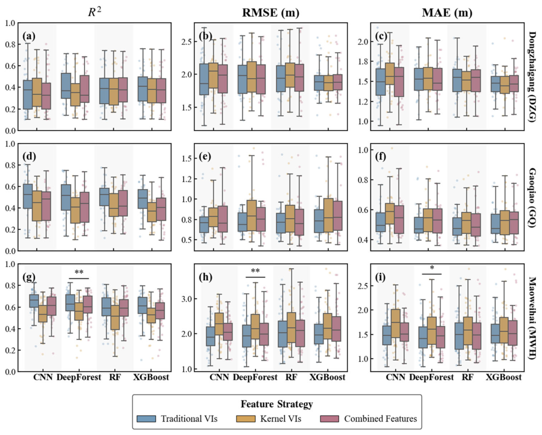
While global benchmarks provide average accuracy snapshots (Table 2), the multi-round spatial cross-validation boxplots (Figure 8) uncover a deeper dimension of model behavior: the distribution stability and error dispersion across localized ecosystems. Across all evaluation tiers, the performance metrics exhibited considerable sensitivity to both architectural choices and regional environmental gradients.

A prominent spatial heterogeneity is evident across the three geographic domains (Hainan-DZG, Gaoqiao-GQ, and Maowei-MWH). Specifically, the absolute retrieval performance and distribution spread varied markedly from site to site, reflecting how underlying canopy structures and background interferences modulate model generalization. In Hainan-DZG (Figure 8a–c) and Gaoqiao-GQ (Figure 8d–f), the boxplots display relatively broad interquartile ranges (IQRs) and extended whiskers across most models, indicating that complex tidal inundation and structural fragmentation induce substantial prediction variability during spatial transfer.

In contrast, within the Maowei-MWH ecosystem (Figure 8g–i), models demonstrated more compact error distributions. Notably, for the DeepForest architecture in MWH (Figure 8g–i), the performance metrics revealed statistically significant variations among feature strategies (indicated by the ** and * significance markers). While the traditional feature configuration (blue boxes) established a robust baseline with competitive median accuracies, the incorporation of kernel-derived and combined features induced measurable shifts in metric distribution and dispersion. This statistical divergence highlights that in mature and semi-closed mangrove stands, tree-based cascade architectures are highly sensitive to feature space transformations, where high-dimensional feature expansions must be carefully balanced against potential collinearity and local variance.

3.3.3. Regional Adaptability and Performance Convergence Under Independent Site Calibration

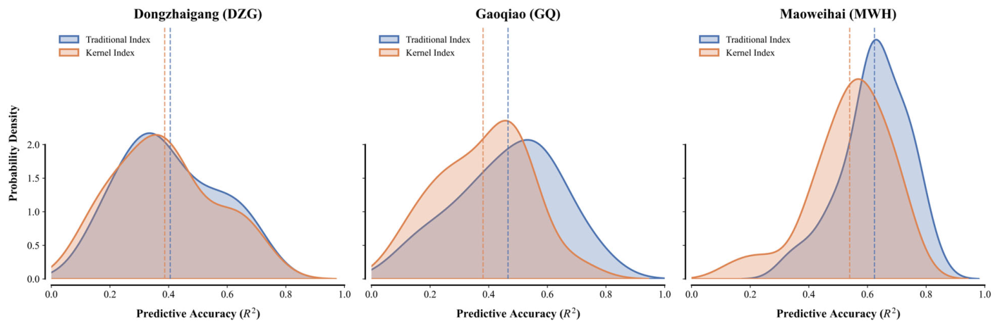
To evaluate the local regional adaptability and structural robustness of the proposed framework across distinct estuarine environments, the DeepForest model was analyzed through independent regionalized modeling across the three heterogeneous study sites: Hainan (DZG), Guangdong (GQ), and Guangxi (MWH). This site-specific validation strategy is essential to verify how effectively feature configurations resolve the distinct spectral-height relationships inherent in diverse estuarine contexts. The probability density distributions (PDDs) of predictive accuracy ($R^2$), derived from 50 randomized iterations using both traditional and kernel-enhanced feature configurations, are visualized in Figure 9.

As illustrated in the probability curves, localized regional calibration established clear and stable performance convergence bounds across all three ecosystems. Notably, within the Guangxi (MWH) study area (right panel), the model achieved the highest overall predictive accuracy, with prominent probability density peaks clustering densely around $0.60$ to $0.65$ and extending toward $0.80$. This superior localized stability corroborates earlier findings from spectral redistribution analyses, confirming that in mature, relatively continuous mangrove stands, the integrated feature-model framework enables tree-based architectures to efficiently capture dense structural variations without suffering from extreme value compression or feature-space stagnation.

In contrast, the probability distributions for Hainan-DZG (left panel) and Gaoqiao-GQ (middle panel) exhibited broader spreads with lower median $R^2$ values, peaking around $0.35$ to $0.45$. These variations directly mirror the persistent environmental hurdles identified in spatial sensitivity analyses—specifically, severe tidal inundation, sparse dwarf patches, and strong background soil/water interference in intertidal zones. While both traditional and kernel index configurations maintain stable performance baselines in these complex zones, localized structural heterogeneity continues to induce non-trivial prediction variance across independent runs.

Ultimately, these regionalized distribution profiles demonstrate that while feature expansions and kernel transformations do not serve as universal boosters for direct spatial transfer, they provide robust local adaptability and reliable non-linear alignment. The high degree of predictive stability across diverse successional stages underscores the practical reliability of the integrated KVI-DeepForest approach for operational mangrove canopy height retrieval within site-specific regional domains.

3.4. Spatial Patterns of Mapped MCH Across Three Mangrove Ecosystems

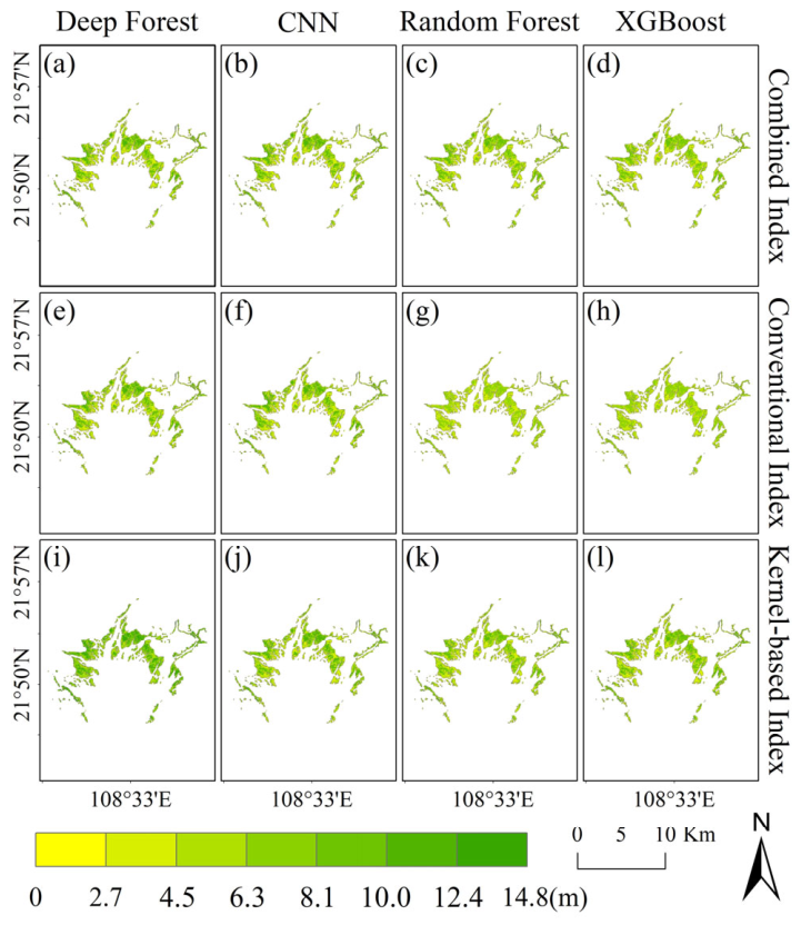
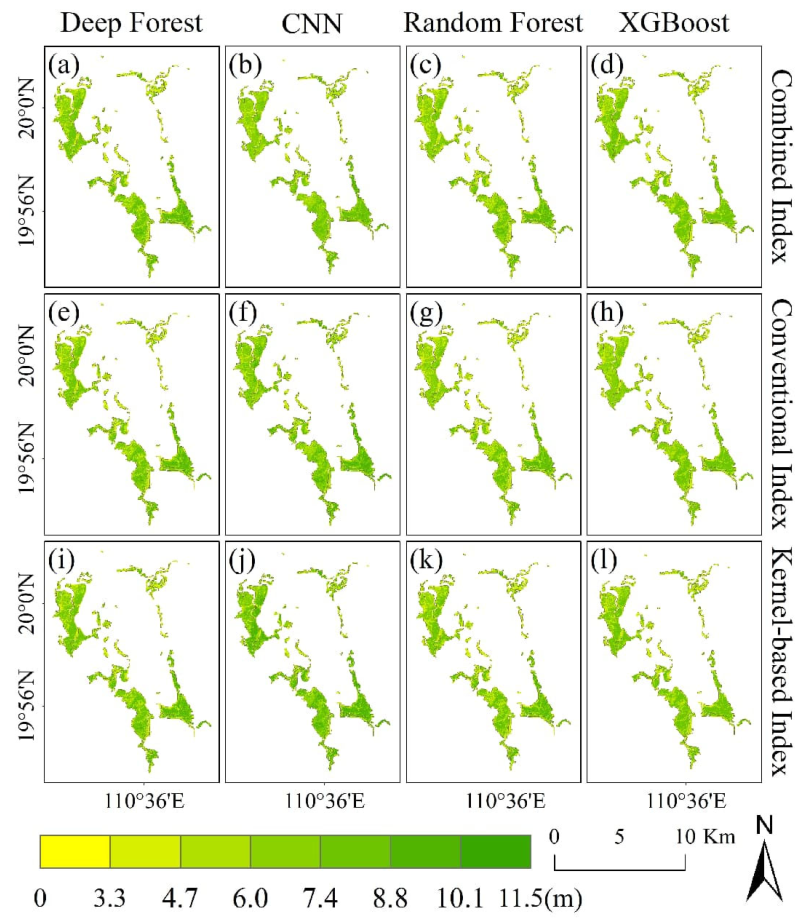
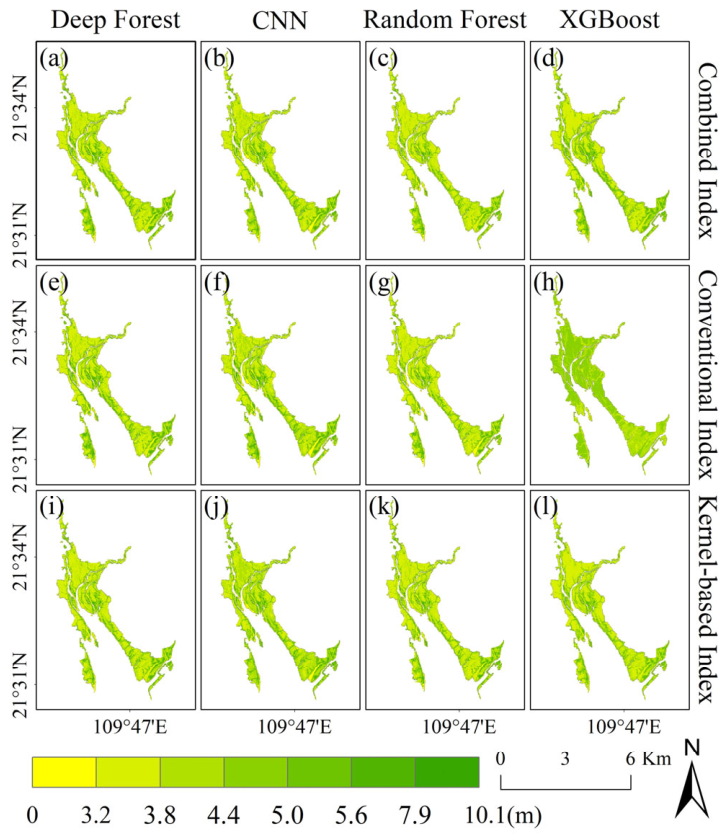
The spatially continuous MCH maps revealed clear differences in canopy-height magnitude and spatial organization among the three mangrove ecosystems (Figure 10, Figure 11 and Figure 12). The mapped height ranges reflected the distinct ecological baselines across sites, with the color scales spanning $0\mathrm{m}$ to $11.5\mathrm{m}$ in DZG, $0\mathrm{m}$ to $10.1\mathrm{m}$ in GQ, and $0\mathrm{m}$ to $14.8\mathrm{m}$ in MWH.

In DZG (Figure 10), predicted MCH showed a relatively continuous spatial structure, with higher canopy values concentrated in mature core stands and riverine zones. Across the model-feature combinations, most mapped pixels fell within the intermediate height classes (approximately $4.7\mathrm{m}$ to $8.8\mathrm{m}$), while localized high-value patches approached the upper limit of $11.5\mathrm{m}$. The spatial patterns exhibited high consistency across different feature sets and algorithms, indicating a strong structural robustness in this regional mapping.

In GQ (Figure 11), the mapped canopy-height range was narrower, with the color scale extending up to $10.1\mathrm{m}$. Most mangrove pixels were visually concentrated within lower-to-intermediate classes (approximately $3.2\mathrm{m}$ to $5.6\mathrm{m}$), and high-canopy patches above $7.9\mathrm{m}$ were spatially sparse. Compared with DZG, the GQ maps exhibited consistent spatial coverage but subdued height contrast, reflecting the stunted structural characteristics typical of this regional environment.

In MWH (Figure 12), the predicted MCH maps reached the highest upper bound among the three sites, extending up to $14.8\mathrm{m}$. The spatial patterns displayed a more heterogeneous arrangement embedded within estuarine boundaries. Most mapped areas appeared within intermediate height classes ($4.5\mathrm{m}$ to $8.1\mathrm{m}$), whereas high-value pixels ($>12.4\mathrm{m}$) were localized in core patches. Overall, spatial predictions remained stable across various feature configurations, reinforcing the reliability of the mapping framework in complex, fragmented estuarine landscapes.

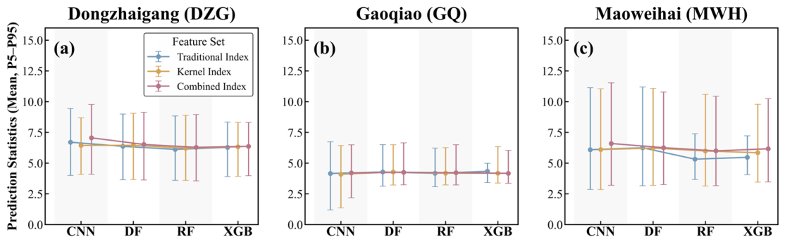
To further dissect how different feature configurations—Traditional, Kernel, and Combined Index—and machine learning architectures interact with site-specific ecological baselines, the statistical distributions (mean and P5–P95 ranges) of predicted MCH were evaluated (Figure 13). As shown in Figure 13a (DZG), predicted mean values remained relatively stable across all algorithms, clustering around 6.0–7.0 m. Notably, all feature configurations under the CNN model yielded elevated P95 upper bounds (approaching 9.5–10.0 m), indicating that convolutional architectures broaden sensitivity to structural extremes. In contrast, Figure 13b (GQ) demonstrates a compressed statistical range, with means stably constrained around 4.0 m and error bounds spanning roughly from 1.2 m to 6.6 m across models, reflecting the homogeneous structural baseline of this region. Critical divergence is evident in Figure 13c (MWH). While Traditional Index configurations under RF and XGB models trend toward lower mean values (5.3–5.5 m), various feature configurations maintain higher baseline means and extend the P95 upper whiskers up to 11.0–11.5 m under CNN and DF architectures. This confirms that advanced architectural and feature transformations effectively alleviate upper-bound feature compression and expand the captured structural range in dense canopy conditions. These statistical trends provide the necessary context for understanding the spatial dispersion patterns analyzed in the subsequent section, where the trade-off between captured structural heterogeneity and algorithmic sensitivity is mapped across the study landscapes.

3.5. Prediction Stability and Dispersion Patterns of Mapped MCH Across Three Mangrove Ecosystems

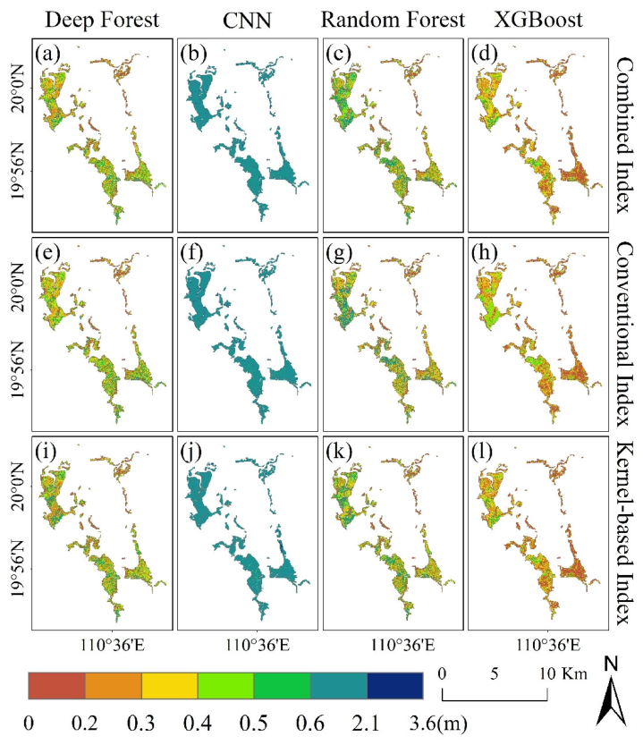
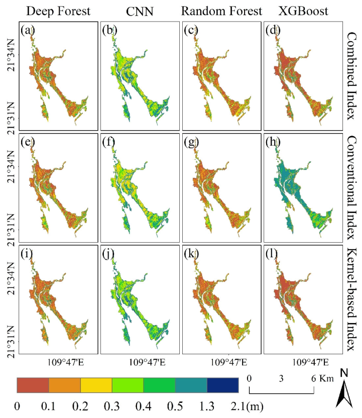
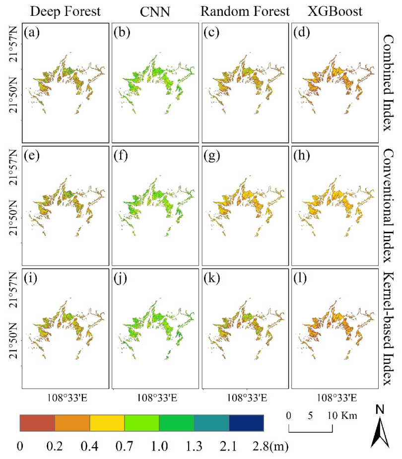
Pixel-level model dispersion across repeated model runs was evaluated using standard deviation maps derived from 50 randomized models (Figure 14, Figure 15 and Figure 16). It is important to note that this pixel-level standard deviation represents ensemble prediction dispersion or sampling variability resulting from different data splits and initialization seeds, rather than a fully calibrated estimate of predictive uncertainty. The dispersion ranges differed clearly among the three study sites, with color-scale upper limits of 3.6 m in DZG, 2.1 m in GQ, and 2.8 m in MWH. This site-level contrast indicates that prediction variability was not uniform across the study domains and was modulated by structural complexity and algorithmic sensitivity to feature perturbations.

In DZG (Figure 14), the spatial distribution of ensemble prediction dispersion revealed a strong model-dependent pattern. Notably, CNN outputs (Figure 14b,f,j) consistently exhibited higher standard deviation values (dominated by cyan classes in the 0.6–2.1 m range) across the spatial extent, indicating greater prediction variance and lower iteration consistency in this mature ecosystem. In contrast, Deep Forest and Random Forest produced more spatially coherent distributions with lower dispersion levels. XGBoost displayed intermediate dispersion with localized patches of elevated variance near forest edges. Furthermore, comparing across rows, the dispersion patterns within the same model showed minimal variation across feature sets (Combined, Conventional, and Kernel-based), suggesting that model architecture exerted a more dominant control on ensemble prediction dispersion than input feature configurations in DZG.

In GQ (Figure 15), the overall dispersion range was compressed to a maximum of 2.1 m. Most models and feature configurations maintained predominantly low standard deviation levels. However, a striking anomaly was observed in XGBoost under conventional feature configurations (Figure 15h), which anomalously displayed an extensive high-dispersion surface, whereas its performance stabilized under combined (Figure 15d) and kernel-based (Figure 15l) configurations. This indicates that conventional index features can induce high algorithmic instability for gradient boosting trees in stunted mangrove environments. Meanwhile, Deep Forest and CNN maintained relatively balanced spatial variance bounds across feature variations, reflecting more robust convergence in linear, strip-like coastal settings.

In MWH (Figure 16), dispersion distributions reflected the highly fragmented nature of this estuarine landscape, with the color scale extending to an upper limit of 2.8 m. A distinct divergence among model architecture was observed. XGBoost outputs (Figure 16d,h,l) predominantly occupied the lower standard-deviation bounds, indicating high iteration consistency across repeated runs in this complex setting. In contrast, Deep Forest, Random Forest, and CNN produced comparatively higher variance surfaces, reflecting greater sensitivity to background mixing between water, exposed sediment, and fragmented vegetation patches. Furthermore, like DZG and GQ, the spatial patterns for each model remained largely invariant across the three feature sets, reinforcing the conclusion that model structure was the primary driver of prediction dispersion.

Notably, the 1D-CNN architecture exhibited a distinct behavioral divergence: while its localized convolutional filters occasionally captured fine-scale feature variations yielding competitive point-level residual metrics in certain subsets, it consistently showed elevated standard deviation values and run-to-run variability across repeated runs (Figure 14b,f,j). This trade-off arises because deep sequence-based architectures are inherently sensitive to minor feature perturbations and edge-pixel noise. When upscaled from discrete footprints to continuous wall-to-wall mapping, such local sensitivity is propagated and amplified across spatial grids, resulting in high prediction variance despite acceptable localized point accuracy. Crucially, a spatially smooth prediction dispersion map or lower standard deviation should not be automatically equated with superior predictive accuracy or absolute reliability, as ensemble dispersion primarily reflects algorithmic robustness against random data splits rather than verified error distributions.

4. Discussion

4.1. Spectral–Structural Mismatch Constrains Optical Retrieval of Mangrove Canopy Height

A central difficulty in MCH retrieval is that canopy height is a vertical structural attribute, whereas optical sensors primarily record horizontal spectral responses from the canopy surface and its background. This spectral–structural mismatch is a fundamental limitation of optical upscaling approaches and explains why LiDAR-derived vertical information has become increasingly important for forest and mangrove height mapping [11,12]. This mismatch is amplified in mangrove ecosystems because canopy reflectance is jointly affected by stand maturity, canopy closure, species composition, tidal inundation, exposed sediments, shadow effects, and forest–water mixed pixels [18,19]. Therefore, MCH cannot be treated as a simple greenness-related variable. This is consistent with the present correlation analysis, which revealed that while multi-source feature sets enhanced correlations (with maximum absolute values reaching up to 0.656 in DZG, 0.453 in GQ, and 0.564 in MWH), individual conventional indices often exhibited limited single-index linear sensitivity or regional sign inversions (e.g., water/moisture indices shifting positive in GQ to negative in DZG and MWH). This weak and spatially variable index–height relationship is ecologically plausible. Global mangrove studies have shown that canopy height is regulated by broad climatic and disturbance gradients rather than by canopy greenness alone. For example, precipitation, temperature, and cyclone frequency explain a large proportion of global variation in maximum mangrove canopy height, while local geomorphology and hydrological conditions further shape regional variability [6].

Kernel-based indices partially address this limitation by transforming band relationships into a nonlinear similarity space, acting as structural stabilizers and non-linear topological enhancements rather than direct accuracy boosters [20]. This approach follows the kNDVI framework, which generalizes conventional vegetation-index formulations by exploiting higher-order relationships among spectral channels [20]. Unlike traditional ratio- or difference-based indices, kernelized indices can redistribute spectrally compressed pixels, especially when conventional indices approach saturation under dense vegetation conditions [17,20,53]. This mechanism is consistent with the broader literature showing that spectral saturation remains a major constraint in estimating high-density vegetation traits such as biomass, leaf area index, and canopy structural attributes [15,17]. However, kernel transformation does not introduce direct vertical measurements; it only modifies the spectral representation provided to the regression model.

It is noteworthy that kernel-based vegetation indices (KVIs) do not consistently yield uniform improvements in global predictive metrics (e.g., $R^2$ or RMSE) across all models and sites. Consequently, the utility of KVIs should be understood as a form of “defensive” performance optimization rather than “offensive” accuracy mining. Although experimental metrics occasionally show localized improvements in global $R^2$ or RMSE, the direct contribution of KVIs to predictive performance is primarily manifested as bias suppression and spatial regularization. In regions prone to systematic under- or overestimation due to upper-bound spectral compression, KVIs reshape the feature manifold, effectively reducing prediction standard deviations and mitigating structural bias without serving as a universal accuracy booster. Specifically, KVIs function primarily as a structural stabilizer that decouples vegetation height from compressed spectral plateaus in high-biomass stands, mitigates background noise induced by water–soil mixed pixels in fragmented estuarine zones, and enhances the spatial consistency and robustness of the predictive models.

A potential skepticism regarding kernel-based feature engineering is whether high-dimensional kernel indices introduce redundant information or simply replicate traditional linear metrics. Our regional correlation and VIF diagnostics explicitly counter this hypothesis. As evidenced by the VIF panels in the correlation matrices, although certain kernel indices exhibit moderate-to-high pairwise correlations (e.g., for 0.78 and 0.76), their corresponding VIF values consistently remain well below critical thresholds (mostly below 5.0). This phenomenon occurs because VIF evaluates the collective multicollinearity across the entire feature space rather than isolated pairwise relationships, confirming that the kernel transformation maps spectral data into a non-linear feature space without inducing severe variance inflation. Consequently, these kernelized indices provide complementary dimensions that assist tree-based ensemble models in resolving vertical heterogeneity without suffering from multicollinearity-driven overfitting.

4.2. Model Performance Reflects a Trade-Off Between Point-Level Accuracy and Spatial Reliability

The comparison among RF, XGBoost, 1D-CNN, and DeepForest indicates that algorithmic structure had a stronger influence on average MCH retrieval accuracy than feature configuration alone. Furthermore, our regional evaluation reveals that the inherent structural heterogeneity and sample distribution profiles across study sites critically modulate model convergence and regional performance consistency. Specifically, the distinct GEDI reference sample configurations—ranging from the unimodal pattern in Gaoqiao (GQ) and the bimodal profile in Dongzhaigang (DZG) to the right-skewed long-tail configuration in Maoweihai (MWH reaching up to 17.6 m)—provide a compelling ecological and machine-learning explanation for regional variations in predictive accuracy (e.g., the elevated $R^2$ observed in MWH). From a methodological perspective, MWH’s broader vertical dynamic range and extended high-stature tail provide a richer and more continuous feature gradient for non-linear learning algorithms. In contrast to narrow or compressed height ranges that easily induce target clipping or gradient starvation during tree-partitioning, a comprehensive structural gradient supplies sufficient training instances across diverse successional stages. This expansive feature space empowers tree ensembles (such as XGBoost and DeepForest) to better resolve extreme biomass values and remedy upper-bound feature compression, underscoring that robust spatial prediction heavily relies on the breadth and representativeness of training sample gradients [54].

Under the traditional index configuration, 1D-CNN achieved competitive baseline footprint-level accuracy (e.g., yielding higher point-level $R^2$ or lower residuals in specific subsets), whereas tree-based models exhibited comparable baseline metrics. When transitioning to kernel-based and combined feature configurations, overall performance experienced a moderate recalibration rather than universal accuracy enhancements across all models. This quantitative reality indicates that while KVIs and multi-source fusions effectively restructure the feature manifold (as verified by VIF and dispersion reductions), they do not function as indiscriminate global accuracy boosters; rather, their quantitative utility is manifested primarily in spatial regularization and structural bias mitigation under complex canopy configurations.

DeepForest and XGBoost exhibit distinct architectural trade-offs in local regional adaptability and spatial stability. As demonstrated by independent regionalized modeling and probability density distributions, localized calibration established clear convergence bounds (such as higher $R^2$ peaks clustering around $0.60$ to $0.65$ in MWH compared to broader spreads in DZG and GQ). In these complex estuarine and intertidal environments, DeepForest and RF generally produced more spatially coherent ensemble dispersion patterns than CNN and certain XGBoost configurations (such as the elevated ensemble dispersion observed in XGBoost under conventional features in GQ). This suggests that cascaded forest ensembles effectively dampen local prediction volatility and handle background water–soil interferences, even where mean-value convergence is secondary to spatial smoothness. The original gcForest framework was proposed precisely to provide deep representation learning through ensemble forests rather than gradient-based neural networks [24].

The behavior of 1D-CNN further clarifies the importance of matching model architecture to predictor structure. A one-dimensional convolutional model assumes meaningful local ordering in the input vector. This assumption is reasonable for spectral curves, waveforms, or time-series signals, but it is less secure for a set of engineered vegetation and water indices whose ordering is not physically continuous. The performance shifts in CNN under different feature configurations suggest that kernelized or engineered indices do not always provide a uniform sequential structure for convolutional feature extraction, requiring traditional index components to maintain stability.

These findings imply that MCH model selection should distinguish between point-level accuracy and map-level reliability, because point-based validation can overestimate the reliability of spatially continuous predictions when spatial dependence is not properly accounted for. XGBoost and DeepForest serve complementary roles depending on whether footprint-level residual minimization or spatial dispersion suppression is prioritized. This distinction is especially important because random train–test splits can underestimate prediction error in spatially autocorrelated ecological data. Spatially structured validation has therefore been recommended when assessing the spatial robustness of geospatial models [51].

The broader implication of this study is that mangrove remote sensing should move beyond extent mapping toward structure-sensitive monitoring. Global Mangrove Watch has substantially improved the capacity to monitor mangrove extent and change from 1996 to 2020, supporting conservation planning and risk assessment [55]. However, mangrove extent alone cannot characterize canopy development, degradation status, restoration trajectories, habitat vertical complexity, or biomass potential. MCH provides a structural layer that links spatial mapping with ecological function.

Recent global products have already demonstrated the value of LiDAR–image fusion for canopy-height mapping. GEDI provides spaceborne waveform measurements of forest vertical structure, while optical, radar, or interferometric predictors provide spatial continuity. Global mangrove canopy-height products have been generated using ICESat-2 and multi-source imagery at $30\mathrm{m}$ resolution, as well as TanDEM-X products calibrated and validated with GEDI at $12\mathrm{m}$ resolution. Our results underscore that engineering, particularly the deployment of KVIs, must be conditioned on landscape-scale ecological constraints: dense closed-canopy systems require spectral redistribution to alleviate upper-bound compression, whereas fragmented estuarine systems demand robust separation of tidal background and vegetation signals.

In high-canopy mangrove stands, feature engineering—specifically the deployment of KVIs—should be conditioned on the target landscape’s structural and hydrological constraints to leverage their feature-stretching and noise-suppression capabilities, rather than being applied as a uniform processing default. Consequently, the selection and evaluation of these features must be informed by local canopy closure, tidal dynamics, and patch fragmentation. Beyond mapping, mangrove forests are among the most carbon-rich coastal ecosystems, where canopy height is a fundamental proxy for biomass and carbon-stock estimation. Given that robust carbon accounting requires integrating species composition, wood density, and belowground parameters, this study offers a structure-sensitive layer that stabilizes canopy height retrieval in heterogeneous mangrove patches. Such reliable structural baseline data are essential for supporting subsequent carbon dynamics assessments and biomass estimations in recovering or fragmented ecosystems where linear optical indices typically falter.

4.3. Limitations and Future Directions

Although this study demonstrates the utility of an integrated GEDI-optical framework for mapping mangrove canopy height, several aspects require further development to enhance its ecological applicability and local regional adaptability.

First, the current framework relies primarily on optical spectral features and kernel-based transformations to spatially upscale GEDI-derived height samples. While optical data and kernel indices provide non-linear feature adjustments that help stabilize predictions against upper-bound feature compression and background noise, they remain indirectly related to vertical canopy structure. In dense mangrove stands, canopy closure continues to constrain the sensitivity of optical signals, whereas in fragmented estuarine landscapes, mixed water–sediment–vegetation pixels complicate the spectral–structural relationship. Furthermore, the multi-year temporal window (spanning from 2023 to 2025) necessitated by persistent cloud cover in sites such as Dongzhaigang (DZG)—despite mitigation via multi-year median compositing—may inherently introduce unresolved phenological noise, inter-annual vegetation growth dynamics, or localized anthropogenic disturbances (such as mangrove clearance or restoration activities) that decouple older footprint observations from concurrent spectral predictors. Future work should therefore incorporate complementary structural predictors, such as Sentinel-1 or ALOS/PALSAR radar backscatter, interferometric height metrics, Sentinel-2 red-edge bands, and multi-seasonal temporal descriptors, to better capture canopy vertical complexity and transient landscape changes [6].

Second, the spatial generalizability and local regional adaptability of the proposed feature-model framework face notable challenges when extrapolated to unseen environmental gradients, as reflected by performance variations across distinct regional test partitions. Although the three study sites capture important contrasts in canopy density, landscape fragmentation, and hydrological backgrounds, significant environmental heterogeneity and distribution shifts among sites constrain the model’s out-of-sample predictive power. Furthermore, mangrove height–spectral relationships vary substantially among river-dominated deltas, carbonate islands, arid coasts, cyclone-prone shorelines, and restoration plantations. Extending the framework through domain adaptation or transfer learning techniques across a broader spectrum of biogeographic and geomorphic settings would allow a more rigorous assessment of the context-dependent utility of kernel-based features, helping to determine whether the observed patterns can be robustly scaled across diverse mangrove systems.

Third, this study focuses on MCH retrieval as a critical structural layer rather than direct biomass or blue-carbon estimation. While canopy height serves as a fundamental proxy for forest vertical structure and supports biomass modeling, accurate carbon-stock estimation requires additional information, including species composition, wood density, stand density, allometric relationships, belowground biomass, soil carbon, and uncertainty propagation. Future studies should consequently couple remote-sensing-derived MCH maps with field inventory data and carbon accounting models, enabling the structure-sensitive mapping framework developed herein to better support biomass estimation and blue-carbon assessments.

Finally, future mangrove height products should be evaluated not only by footprint-level prediction accuracy but also by spatial reliability, ensemble dispersion distribution, and ecological interpretability. The present results indicate that the model yielding the highest point-level accuracy is not necessarily the one with the most spatially stable prediction surface, thereby highlighting a trade-off between residual minimization and dispersion suppression. This trade-off is particularly critical for coastal management, as forest edges, tidal channels, fragmented patches, and restoration zones typically represent areas of highest mapping dispersion and greatest sensitivity in management decision-making. Consequently, future research should develop comprehensive evaluation strategies that jointly account for accuracy, ensemble dispersion, spatial robustness, and ecological relevance, rather than relying on any single performance metric.

5. Conclusions

This study evaluated the utility of kernel-based spectral features for GEDI–Sentinel-2 and Sentinel-1 MCH retrieval across three representative mangrove ecosystems in South China. Single optical and radar-derived indices exhibited limited linear sensitivity to GEDI-derived MCH. Although the traditional-index 1D-CNN achieved a competitive baseline point-level accuracy (e.g., yielding higher $R^2$ under conventional features), overall performance exhibited a moderate recalibration rather than universal accuracy enhancements when transitioning to kernel-based and combined configurations. Rather than serving as universal accuracy boosters, kernel-based transformations functioned as adaptive feature-space regularizers and mechanisms for feature-compression alleviation, redistributing spectral-radar signals to suppress signal compression in dense canopies and reduce background noise in fragmented landscapes. Their value was manifested in localized spatial regularization and bias suppression rather than massive leaps in global numerical accuracy.

Furthermore, model comparison demonstrated a clear trade-off between point-level accuracy and spatial reliability. XGBoost remained a strong benchmark for minimizing footprint-level residuals, whereas the DeepForest framework offered enhanced spatial stability and reduced ensemble prediction dispersion, particularly in complex canopy configurations. However, the evaluation across unseen environmental gradients also revealed that spatial generalizability and local regional adaptability remain challenging, as significant environmental heterogeneity and data distribution shifts among sites constrain out-of-sample predictive power. Spatial mapping further revealed distinct canopy-height and ensemble dispersion patterns among DZG, GQ, and MWH, confirming that MCH inversion performance is modulated by regional geomorphology, tidal dynamics, and localized environmental contexts.

Ultimately, these findings indicate that mangrove canopy height retrieval should be evaluated through the dual lens of prediction accuracy and spatial reliability. Kernel-based features are best interpreted as adaptive topological supplements to traditional indices, and their operational effectiveness depends strictly on local canopy density, background complexity, and model architecture. It should be noted that these findings are based on representative ecosystems along the South China coast; the proposed framework should be applied with caution in other global mangrove sub-types, as varying geomorphic and biogeographic conditions may necessitate further model calibration. Moving forward, addressing spatial adaptation challenges across heterogeneous domains through domain adaptation or advanced transfer learning strategies will be critical. Collectively, the synergy between kernelized feature engineering and structure-sensitive modeling offers a robust and adaptive technical foundation for mapping complex coastal biophysical parameters in these study regions, providing reliable structural support for the ecological assessment and habitat management of mangrove ecosystems.

References

1. Alongi, D.M. Carbon Cycling and Storage in Mangrove Forests. Annu. Rev. Mar. Sci. 2014, 6, 195–219. [Google Scholar] [CrossRef] [Scilit] [PubMed]
2. Donato, D.C.; Kauffman, J.B.; Murdiyarso, D.; Kurnianto, S.; Stidham, M.; Kanninen, M. Mangroves among the most carbon-rich forests in the tropics. Nat. Geosci. 2011, 4, 293–297. [Google Scholar] [CrossRef] [Scilit]
3. McLeod, E.; Chmura, G.L.; Bouillon, S.; Salm, R.; Björk, M.; Duarte, C.M.; Lovelock, C.E.; Schlesinger, W.H.; Silliman, B.R. A blueprint for blue carbon: Toward an improved understanding of the role of vegetated coastal habitats in sequestering CO2. Front. Ecol. Environ. 2011, 9, 552–560. [Google Scholar] [CrossRef] [Scilit]
4. Lagomasino, D.; Fatoyinbo, T.; Lee, S.; Feliciano, E.; Trettin, C.; Simard, M. A Comparison of Mangrove Canopy Height Using Multiple Independent Measurements from Land, Air, and Space. Remote Sens. 2016, 8, 327. [Google Scholar] [CrossRef] [Scilit] [PubMed]
5. Feliciano, E.A.; Wdowinski, S.; Potts, M.D.; Lee, S.-K.; Fatoyinbo, T.E. Estimating Mangrove Canopy Height and Above-Ground Biomass in the Everglades National Park with Airborne LiDAR and TanDEM-X Data. Remote Sens. 2017, 9, 702. [Google Scholar] [CrossRef] [Scilit]
6. Simard, M.; Fatoyinbo, L.; Smetanka, C.; Rivera-Monroy, V.H.; Castañeda-Moya, E.; Thomas, N.; Van Der Stocken, T. Mangrove canopy height globally related to precipitation, temperature and cyclone frequency. Nat. Geosci. 2019, 12, 40–45. [Google Scholar] [CrossRef] [Scilit]
7. Simard, M.; Fatoyinbo, L.; Thomas, N.M.; Stovall, A.E.; Parra, A.; Barenblitt, A.; Bunting, P.; Hajnsek, I. A New Global Mangrove Height Map with a 12 meter spatial resolution. Sci. Data 2025, 12, 15. [Google Scholar] [CrossRef] [Scilit] [PubMed]
8. Yu, J.; Nie, S.; Liu, W.; Zhu, X.; Sun, Z.; Li, J.; Wang, C.; Xi, X.; Fan, H. Mapping global mangrove canopy height by integrating Ice, Cloud, and Land Elevation Satellite-2 photon-counting LiDAR data with multi-source images. Sci. Total Environ. 2024, 939, 173487. [Google Scholar] [CrossRef] [Scilit] [PubMed]
9. Pham, T.D.; Yokoya, N.; Bui, D.T.; Yoshino, K.; Friess, D.A. Remote Sensing Approaches for Monitoring Mangrove Species, Structure, and Biomass: Opportunities and Challenges. Remote Sens. 2019, 11, 230. [Google Scholar] [CrossRef] [Scilit]
10. Pradisty, N.A.; Schlund, M.; Horstman, E.M.; Willemen, L. Estimating canopy height and aboveground biomass in tropical mangrove restoration areas through multisource remote sensing. Ecol. Inform. 2025, 92, 103522. [Google Scholar] [CrossRef] [Scilit]
11. Dubayah, R.; Blair, J.B.; Goetz, S.; Fatoyinbo, L.; Hansen, M.; Healey, S.; Hofton, M.; Hurtt, G.; Kellner, J.; Luthcke, S.; et al. The Global Ecosystem Dynamics Investigation: High-resolution laser ranging of the Earth’s forests and topography. Sci. Remote Sens. 2020, 1, 100002. [Google Scholar] [CrossRef] [Scilit]
12. Potapov, P.; Li, X.; Hernandez-Serna, A.; Tyukavina, A.; Hansen, M.C.; Kommareddy, A.; Pickens, A.; Turubanova, S.; Tang, H.; Silva, C.E.; et al. Mapping global forest canopy height through integration of GEDI and Landsat data. Remote Sens. Environ. 2021, 253, 112165. [Google Scholar] [CrossRef] [Scilit]
13. Lang, N.; Jetz, W.; Schindler, K.; Wegner, J.D. A high-resolution canopy height model of the Earth. Nat. Ecol. Evol. 2023, 7, 1778–1789. [Google Scholar] [CrossRef] [Scilit] [PubMed]
14. Yulianto, F.; Kushardono, D.; Budhiman, S.; Nugroho, G.; Chulafak, G.A.; Dewi, E.K.; Pambudi, A.I. Evaluation of the Threshold for an Improved Surface Water Extraction Index Using Optical Remote Sensing Data. Sci. World J. 2022, 2022, 4894929. [Google Scholar] [CrossRef] [Scilit] [PubMed]
15. Mutanga, O.; Masenyama, A.; Sibanda, M. Spectral saturation in the remote sensing of high-density vegetation traits: A systematic review of progress, challenges, and prospects. ISPRS J. Photogramm. Remote Sens. 2023, 198, 297–309. [Google Scholar] [CrossRef] [Scilit]
16. Feyisa, G.L.; Meilby, H.; Fensholt, R.; Proud, S.R. Automated Water Extraction Index: A new technique for surface water mapping using Landsat imagery. Remote Sens. Environ. 2014, 140, 23–35. [Google Scholar] [CrossRef] [Scilit]
17. Wang, Q.; Moreno-Martínez, Á.; Muñoz-Marí, J.; Campos-Taberner, M.; Camps-Valls, G. Estimation of vegetation traits with kernel NDVI. ISPRS J. Photogramm. Remote Sens. 2023, 195, 408–417. [Google Scholar] [CrossRef] [Scilit]
18. Kuenzer, C.; Bluemel, A.; Gebhardt, S.; Quoc, T.V.; Dech, S. Remote Sensing of Mangrove Ecosystems: A Review. Remote Sens. 2011, 3, 878–928. [Google Scholar] [CrossRef] [Scilit]
19. Pimple, U.; Simonetti, D.; Leadprathom, K.; Pungkul, S.; Pravinvongvuthi, T.; Berger, U.; Gond, V. Tracking mangrove ecosystem dynamics: A remote sensing approach for species classification and conservation assessment. Glob. Ecol. Conserv. 2025, 63, e03865. [Google Scholar] [CrossRef] [Scilit]
20. Camps-Valls, G.; Campos-Taberner, M.; Moreno-Martínez, A.; Walther, S.; Duveiller, G.; Cescatti, A.; Mahecha, M.D.; Muñoz-Marí, J.; García-Haro, F.J.; Guanter, L.; et al. A unified vegetation index for quantifying the terrestrial biosphere. Sci. Adv. 2021, 7, eabc7447. [Google Scholar] [CrossRef] [Scilit] [PubMed]
21. Belgiu, M.; Drăguţ, L. Random forest in remote sensing: A review of applications and future directions. ISPRS J. Photogramm. Remote Sens. 2016, 114, 24–31. [Google Scholar] [CrossRef] [Scilit]
22. Chen, T.; Guestrin, C. XGBoost. In Proceedings of the 22nd ACM SIGKDD International Conference on Knowledge Discovery and Data Mining, San Francisco, CA, USA, 13–17 August 2016; pp. 785–794. [Google Scholar]
23. Utkin, L.V.; Meldo, A.A.; Konstantinov, A.V. Deep Forest as a framework for a new class of machine-learning models. Natl. Sci. Rev. 2019, 6, 186–187. [Google Scholar] [CrossRef] [Scilit] [PubMed]
24. Zhou, Z.H.; Feng, J. Deep forest. Natl. Sci. Rev. 2019, 6, 74–86. [Google Scholar] [CrossRef] [Scilit] [PubMed]
25. Kattenborn, T.; Schiefer, F.; Frey, J.; Feilhauer, H.; Mahecha, M.D.; Dormann, C.F. Spatially autocorrelated training and validation samples inflate performance assessment of convolutional neural networks. ISPRS Open J. Photogramm. Remote Sens. 2022, 5, 100018. [Google Scholar] [CrossRef] [Scilit]
26. Lang, N.; Kalischek, N.; Armston, J.; Schindler, K.; Dubayah, R.; Wegner, J.D. Global canopy height regression and uncertainty estimation from GEDI LIDAR waveforms with deep ensembles. Remote Sens. Environ. 2022, 268, 112760. [Google Scholar] [CrossRef] [Scilit]
27. Chen, B.; Xiao, X.; Li, X.; Pan, L.; Doughty, R.; Ma, J.; Dong, J.; Qin, Y.; Zhao, B.; Wu, Z.; et al. A mangrove forest map of China in 2015: Analysis of time series Landsat 7/8 and Sentinel-1A imagery in Google Earth Engine cloud computing platform. ISPRS J. Photogramm. Remote Sens. 2017, 131, 104–120. [Google Scholar] [CrossRef] [Scilit]
28. Xia, Q.; Qin, C.-Z.; Li, H.; Huang, C.; Su, F.-Z. Mapping Mangrove Forests Based on Multi-Tidal High-Resolution Satellite Imagery. Remote Sens. 2018, 10, 1343. [Google Scholar] [CrossRef] [Scilit]
29. Zhao, D.; Zhang, Y.; Wang, J.; Zhen, J.; Shen, Z.; Xiang, K.; Xiang, H.; Wang, Y.; Wu, G. Spatiotemporal dynamics and geo-environmental factors influencing mangrove gross primary productivity during 2000–2020 in Gaoqiao Mangrove Reserve, China. For. Ecosyst. 2023, 10, 100137. [Google Scholar] [CrossRef] [Scilit]
30. Ming, X.; Tian, Y.; Zhang, Q.; Zhang, Y.; Tao, J.; Lin, J. Coupling ICESat-2 and Sentinel-2 data for inversion of mangrove tidal flat to predict future distribution pattern of mangroves. Int. J. Appl. Earth Obs. Geoinf. 2025, 136, 104398. [Google Scholar] [CrossRef] [Scilit]
31. Huete, A.R. A soil-adjusted vegetation index (SAVI). Remote Sens. Environ. 1988, 25, 295–309. [Google Scholar] [CrossRef] [Scilit]
32. Huete, A.; Didan, K.; Miura, T.; Rodriguez, E.P.; Gao, X.; Ferreira, L.G. Overview of the radiometric and biophysical performance of the MODIS vegetation indices. Remote Sens. Environ. 2002, 83, 195–213. [Google Scholar] [CrossRef] [Scilit]
33. McFeeters, S.K. The use of the Normalized Difference Water Index (NDWI) in the delineation of open water features. Int. J. Remote Sens. 1996, 17, 1425–1432. [Google Scholar] [CrossRef] [Scilit]
34. Breiman, L. Random forests. Mach. Learn. 2001, 45, 5–32. [Google Scholar] [CrossRef] [Scilit]
35. Jamaluddin, I.; Chen, Y.-N.; Ayudyanti, A.G.; Fan, K.-C. Exploring red-edge spectral indices for mangrove canopy height mapping using random forest regression with Sentinel-2 and spaceborne GEDI LiDAR data. In Land Surface and Cryosphere Remote Sensing V; SPIE: Bellingham, WA, USA, 2025. [Google Scholar]
36. Hemati, M.; Mahdianpari, M.; Shiri, H.; Mohammadimanesh, F. Integrating SAR and Optical Data for Aboveground Biomass Estimation of Coastal Wetlands Using Machine Learning: Multi-Scale Approach. Remote Sens. 2024, 16, 831. [Google Scholar] [CrossRef] [Scilit]
37. Farr, T.G.; Rosen, P.A.; Caro, E.; Crippen, R.; Duren, R.; Hensley, S.; Kobrick, M.; Kobrick, M.; Paller, M.; Rodriguez, E.; et al. The Shuttle Radar Topography Mission. Rev. Geophys. 2007, 45, RG2004. [Google Scholar] [CrossRef] [Scilit]
38. Sharifi, A.; Felegari, S.; Tariq, A. Mangrove forests mapping using Sentinel-1 and Sentinel-2 satellite images. Arab. J. Geosci. 2022, 15, 1593. [Google Scholar] [CrossRef] [Scilit]
39. Huete, A.; Justice, C.; Liu, H. Development of vegetation and soil indices for MODIS-EOS. Remote Sens. Environ. 1994, 49, 224–234. [Google Scholar] [CrossRef] [Scilit]
40. Xu, H. Modification of normalised difference water index (NDWI) to enhance open water features in remotely sensed imagery. Int. J. Remote Sens. 2006, 27, 3025–3033. [Google Scholar] [CrossRef] [Scilit]
41. Gitelson, A.A.; Kaufman, Y.J.; Stark, R.; Rundquist, D. Novel algorithms for remote estimation of vegetation fraction. Remote Sens. Environ. 2002, 80, 76–87. [Google Scholar] [CrossRef] [Scilit]
42. Rikimaru, A.; Roy, P.S.; Miyatake, S. Tropical forest cover density mapping. Trop. Ecol. 2002, 43, 39–47. [Google Scholar]
43. Penuelas, J.; Baret, F.; Filella, I. Semi-empirical indices to assess carotenoids/chlorophyll a ratio from leaf spectral reflectance. Photosynthetica 1995, 31, 221–230. [Google Scholar]
44. Lymburner, L.; Beggs, P.J.; Jacobson, C.R. Estimation of canopy-average surface-specific leaf area using Landsat TM data. Photogramm. Eng. Remote Sens. 2000, 66, 183–191. [Google Scholar]
45. Meyer, G.E.; Neto, J.C. Verification of color vegetation indices for automated crop imaging applications. Comput. Electron. Agric. 2008, 63, 282–293. [Google Scholar] [CrossRef] [Scilit]
46. Attema, E.P.W.; Ulaby, F.T. Vegetation modeled as a water cloud. Radio Sci. 1978, 13, 357–364. [Google Scholar] [CrossRef] [Scilit]
47. O’Brien, R.M. A Caution Regarding Rules of Thumb for Variance Inflation Factors. Qual. Quant. 2007, 41, 673–690. [Google Scholar] [CrossRef] [Scilit]
48. Wang, J.; Shen, X.; Cao, L. Upscaling Forest Canopy Height Estimation Using Waveform-Calibrated GEDI Spaceborne LiDAR and Sentinel-2 Data. Remote Sens. 2024, 16, 2138. [Google Scholar] [CrossRef] [Scilit]
49. Lei, R.; Fang, Y.; Du, C.; Zhou, J.; Hang, S.; Xiang, H. Navigating yield-density trade-offs in maize production: A Bayesian-ML framework for uncertainty attribution and management. Field Crops Res. 2026, 342, 110480. [Google Scholar] [CrossRef] [Scilit]
50. Correndo, A.A.; Tremblay, N.; Coulter, J.A.; Ruiz-Diaz, D.; Franzen, D.; Nafziger, E.; Prasad, V.; Rosso, L.H.M.; Steinke, K.; Du, J.; et al. Unraveling uncertainty drivers of the maize yield response to nitrogen: A Bayesian and machine learning approach. Agric. For. Meteorol. 2021, 311, 108668. [Google Scholar] [CrossRef] [Scilit]
51. Ploton, P.; Mortier, F.; Réjou-Méchain, M.; Barbier, N.; Picard, N.; Rossi, V.; Dormann, C.; Cornu, G.; Viennois, G.; Bayol, N.; et al. Spatial validation reveals poor predictive performance of large-scale ecological mapping models. Nat. Commun. 2020, 11, 4540. [Google Scholar] [CrossRef] [Scilit] [PubMed]
52. Fayad, I.; Ienco, D.; Baghdadi, N.; Gaetano, R.; Alvares, C.A.; Stape, J.L.; Scolforo, H.F.; Le Maire, G. A CNN-based approach for the estimation of canopy heights and wood volume from GEDI waveforms. Remote Sens. Environ. 2021, 265, 112652. [Google Scholar] [CrossRef] [Scilit]
53. Pérez-Suay, A.; Amorós-López, J.; Gómez-Chova, L.; Laparra, V.; Muñoz-Marí, J.; Camps-Valls, G. Randomized kernels for large scale Earth observation applications. Remote Sens. Environ. 2017, 202, 54–63. [Google Scholar] [CrossRef] [Scilit]
54. Ren, C.; Jiang, H.; Xi, Y.; Liu, P.; Li, H. Quantifying Temperate Forest Diversity by Integrating GEDI LiDAR and Multi-Temporal Sentinel-2 Imagery. Remote Sens. 2023, 15, 375. [Google Scholar] [CrossRef] [Scilit]
55. Bunting, P.; Rosenqvist, A.; Lucas, R.M.; Rebelo, L.M.; Hilarides, L.; Thomas, N.; Hardy, A.; Itoh, T.; Shimada, M.; Finlayson, C.M. The Global Mangrove Watch—A New 2010 Global Baseline of Mangrove Extent. Remote Sens. 2018, 10, 1669. [Google Scholar] [CrossRef] [Scilit]
Figure 1. Schematic map of the study areas (I. Dongzhaigang, II. Gaoqiao, III. Maoweihai) along the South China coast. The color gradients represent the DEM elevation (in meters), and the green dots represent the GEDI sample sites.
Remotesensing 18 02834 g001
Figure 2. Distribution of GEDI-derived canopy height (MCH) samples for the three study sites. The blue bars represent the frequency histograms, and the blue solid curves represent the probability density functions. N , Min, and Max denote the sample size, minimum canopy height, and maximum canopy height, respectively.
Remotesensing 18 02834 g002
Figure 3. Multivariate collinearity and correlation matrix for the MWH region. Note: *** p < 0.001 and * p < 0.05 indicate statistical significance.
Remotesensing 18 02834 g003
Figure 4. Multivariate collinearity and correlation matrix for the GQ region. Note: *** p < 0.001 indicates statistical significance.
Remotesensing 18 02834 g004
Figure 5. Multivariate collinearity and correlation matrix for the DZG region. Note: *** p < 0.001 indicates statistical significance.
Remotesensing 18 02834 g005
Figure 6. Pearson correlation analysis between mangrove canopy height (MCH) and remote sensing indices across the three study sites (Dongzhaigang, Gaoqiao, and Maoweihai). Core vegetation indices exhibit consistent positive correlations with canopy height in well-developed mangrove ecosystems ( r ranging from 0.321 to 0.656, all p < 0.05 ). Note: Asterisks (*) denote statistically significant correlations ( p < 0.05 ).
Remotesensing 18 02834 g006
Figure 7. Statistical distributions of traditional NDVI and proposed kNDVI across three study sites. The red and blue colors represent the kernel index and traditional index, respectively. The solid curves denote probability density functions, and the vertical dashed lines indicate the mean values.
Remotesensing 18 02834 g007
Figure 8. Statistical distribution of predictive performance across study sites and feature configurations. Specifically: (a) R 2 , (b) RMSE, and (c) MAE at the Dongzhaigang (DZG) site; (d) R 2 , (e) RMSE, and (f) MAE at the Gaoqiao (GQ) site; and (g) R 2 , (h) RMSE, and (i) MAE at the Maowei Sea (MWH) site. Box plots illustrate performance distributions across different machine learning models and feature strategies (Traditional VIs, Kernel VIs, and Combined Features). Note: The alternating background shading is used to visually separate different machine learning models. Asterisks denote statistical significance derived from paired significance tests (e.g., Wilcoxon signed-rank tests or t -tests), where * p < 0.05 and ** p < 0.01 indicate significant differences, respectively.
Remotesensing 18 02834 g008
Figure 9. Probability density distributions of prediction performance ( R 2 ) for the DeepForest model under traditional and kernel index configurations across the three mangrove study areas (Hainan, Gaoqiao, and Maoweihai). The vertical dashed lines represent the mean values of the corresponding distributions.
Remotesensing 18 02834 g009
Figure 10. Spatial distribution of predicted means MCH in Dongzhaigang (DZG) across different models and feature sets. (a) Deep Forest with Combined Index; (b) CNN with Combined Index; (c) Random Forest with Combined Index; (d) XGBoost with Combined Index; (e) Deep Forest with Conventional Index; (f) CNN with Conventional Index; (g) Random Forest with Conventional Index; (h) XGBoost with Conventional Index; (i) Deep Forest with Kernel-based Index; (j) CNN with Kernel-based Index; (k) Random Forest with Kernel-based Index; (l) XGBoost with Kernel-based Index.
Remotesensing 18 02834 g010
Figure 11. Spatial distribution of predicted mean MCH in Gaoqiao (GQ) across different models and feature sets. (a) Deep Forest with Combined Index; (b) CNN with Combined Index; (c) Random Forest with Combined Index; (d) XGBoost with Combined Index; (e) Deep Forest with Conventional Index; (f) CNN with Conventional Index; (g) Random Forest with Conventional Index; (h) XGBoost with Conventional Index; (i) Deep Forest with Kernel-based Index; (j) CNN with Kernel-based Index; (k) Random Forest with Kernel-based Index; (l) XGBoost with Kernel-based Index.
Remotesensing 18 02834 g011
Figure 12. Spatial distribution of predicted mean MCH in Maowei Sea (MWH) across different models and feature sets. (a) Deep Forest with Combined Index; (b) CNN with Combined Index; (c) Random Forest with Combined Index; (d) XGBoost with Combined Index; (e) Deep Forest with Conventional Index; (f) CNN with Conventional Index; (g) Random Forest with Conventional Index; (h) XGBoost with Conventional Index; (i) Deep Forest with Kernel-based Index; (j) CNN with Kernel-based Index; (k) Random Forest with Kernel-based Index; (l) XGBoost with Kernel-based Index.
Remotesensing 18 02834 g012
Figure 13. Statistical distributions of predicted mangrove canopy height (MCH)—represented by mean values and P5–P95 percentile dispersion intervals—across different machine learning algorithms and feature configurations in three study sites. The alternating background shading is used to visually distinguish different model groups. The blue, yellow, and pink lines represent the Traditional Index, Kernel Index, and Combined Index, respectively.
Remotesensing 18 02834 g013
Figure 14. Ensemble prediction dispersion (standard deviation) maps of MCH inversion in Dongzhaigang (DZG) across different models and feature sets. (a) Deep Forest with Combined Index; (b) CNN with Combined Index; (c) Random Forest with Combined Index; (d) XGBoost with Combined Index; (e) Deep Forest with Conventional Index; (f) CNN with Conventional Index; (g) Random Forest with Conventional Index; (h) XGBoost with Conventional Index; (i) Deep Forest with Kernel-based Index; (j) CNN with Kernel-based Index; (k) Random Forest with Kernel-based Index; (l) XGBoost with Kernel-based Index.
Remotesensing 18 02834 g014
Figure 15. Ensemble prediction dispersion (standard deviation) maps of MCH inversion in Gaoqiao (GQ) across different models and feature sets. (a) Deep Forest with Combined Index; (b) CNN with Combined Index; (c) Random Forest with Combined Index; (d) XGBoost with Combined Index; (e) Deep Forest with Conventional Index; (f) CNN with Conventional Index; (g) Random Forest with Conventional Index; (h) XGBoost with Conventional Index; (i) Deep Forest with Kernel-based Index; (j) CNN with Kernel-based Index; (k) Random Forest with Kernel-based Index; (l) XGBoost with Kernel-based Index.
Remotesensing 18 02834 g015
Figure 16. Ensemble prediction dispersion (standard deviation) maps of MCH inversion in Maowei Sea (MWH) across different models and feature sets. (a) Deep Forest with Combined Index; (b) CNN with Combined Index; (c) Random Forest with Combined Index; (d) XGBoost with Combined Index; (e) Deep Forest with Conventional Index; (f) CNN with Conventional Index; (g) Random Forest with Conventional Index; (h) XGBoost with Conventional Index; (i) Deep Forest with Kernel-based Index; (j) CNN with Kernel-based Index; (k) Random Forest with Kernel-based Index; (l) XGBoost with Kernel-based Index.
Remotesensing 18 02834 g016