Landslide Susceptibility Modeling Constrained by Multi-Scale Polygon Sampling and InSAR Deformation for High-Relief Mountainous Areas: A Case Study in the Upper Jinsha River, Southwest China

Highlights

• A multi-scale polygon-based landslide inventory with information about 3831 landslides in the upper Jinsha River.
• A novel integrating surface deformation RF-OFR LSA framework.
• Fluvial incision and precipitation control landslide occurrence and spatial distribution.
• Multi-scale sampling reduces spatial errors and preserves the heterogeneity of the landslide.
• The provision of a transferable methodology for LSA in high-relief mountainous regions.

What are the main findings?

• The integrated RF-OFR framework combining multi-scale polygon sampling and surface deformation constraints outperforms single and hybrid benchmark models, reaching an AUC of 0.906; fluvial incision, terrain relief and precipitation dominate landslide distribution, while high-susceptibility zones align with river valleys, active faults and persistent surface deformation areas.
• The multi-scale polygon-based sampling strategy captures landslide spatial heterogeneity far better than conventional single-scale point sampling, effectively eliminating sampling bias and lowering evaluation uncertainties in high-relief mountain terrain.

What are the implications of the main findings?

• The proposed modeling workflow clarifies how multi-scale spatial sampling and dynamic surface deformation data jointly improve landslide susceptibility mapping, offering a robust technical scheme for geohazard assessment in rugged plateau mountainous regions.
• This refined assessment method can support regional landslide risk prevention, disaster mitigation and provide a rational layout of major infrastructure projects along river basins on the Tibetan Plateau.

Abstract

The Upper Jinsha River region on the southeastern Tibetan Plateau is characterized by intense tectonic activity, extreme topographic relief, and widespread large-scale landslides, which pose significant threats to communities, transportation networks and major infrastructure. However, accurate landslide susceptibility assessment in high-relief mountainous terrain remains challenging. Conventional methods rely on point-based sampling and static environmental factors, which fail to capture the spatial heterogeneity of large landslides and adequately represent the influence of continuous surface deformation on landslide evolution, resulting in considerable uncertainty and limited predictive accuracy. To address these issues, this study established a polygon-based landslide inventory comprising 3831 landslides and developed an improved susceptibility assessment framework integrating multi-scale polygon-based sampling with InSAR-derived surface deformation constraints. By coupling the Random Forest (RF) and Optimized Frequency Ratio (OFR) models, quantitative susceptibility assessment and model validation were conducted. The results show that the integrated RF-OFR model achieved the best predictive performance, with an Area Under the Curve (AUC) of 0.906, representing improvements of 6.0%, 4.2%, and 2.7% over the conventional FR, RF-FR, and OFR models, respectively. Fluvial incision, terrain relief, and precipitation were identified as the dominant conditioning factors controlling regional landslide occurrence. High-susceptibility zones are primarily distributed along the Jinsha River and deeply incised tributary valleys, showing strong spatial agreement with active fault zones and persistent surface deformation. Compared with conventional single-scale point sampling, the proposed multi-scale polygon sampling strategy more effectively represents the spatial characteristics of large landslides in high-relief mountain regions, reduces sampling bias and incorporating InSAR-derived deformation information further enhances the identification of actively deforming slopes, demonstrating the value of integrating dynamic surface deformation with conventional environmental factors in landslide susceptibility modeling. The proposed framework provides an effective approach for regional landslide susceptibility assessment and can support hazard identification and risk-informed infrastructure and land use planning in high-relief mountainous regions.

1. Introduction

Landslides are among the most destructive geological hazards in mountainous regions worldwide. Along the eastern margin of the Tibetan Plateau, intense tectonic activity, deep fluvial incision, and extreme climatic conditions have promoted the widespread development of large landslides. Many of these landslides undergo prolonged deformation before catastrophic failure, generating landslide–river blockage–dam breach hazard chains that pose severe threats to major engineering projects and densely populated river valleys [1,2].

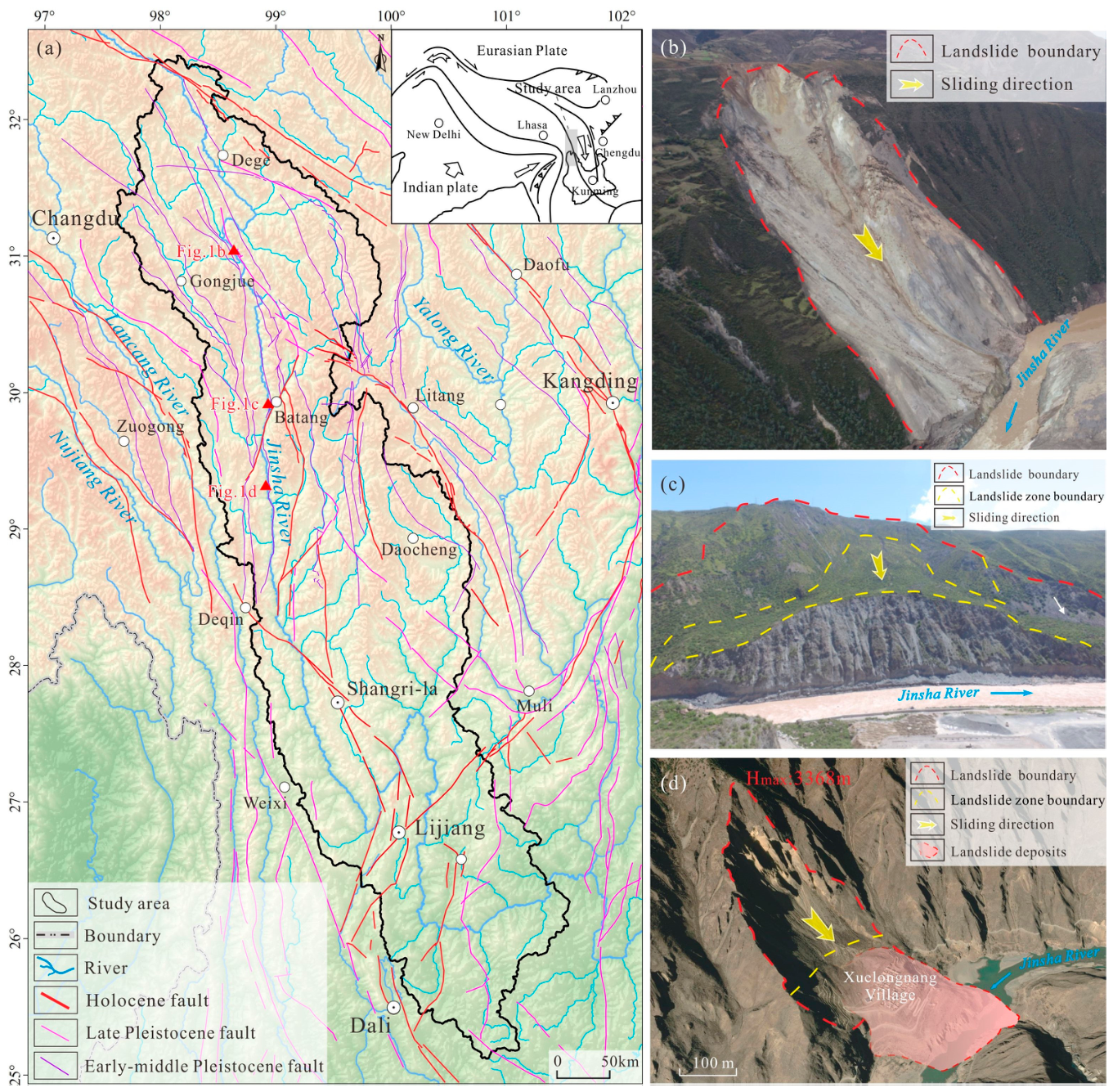
The upper Jinsha River, located along the southeastern margin of the Tibetan Plateau, is characterized by dense active fault systems, frequent seismic activity, and intense fluvial incision, making it one of the regions with the highest concentrations of large landslides in China. According to the classification system proposed by Varnes [3] and Hungr [4], these landslides are mainly categorized as slides, including rotational and translational slides, which are also the main types of subsequent landslide inventories. In recent years, the rapid development of major infrastructure projects, including the Sichuan–Tibet Railway, cascade hydropower stations, and transportation corridors, has substantially increased regional exposure to landslide hazards. Landslides in high-relief mountainous regions often experience progressive deformation processes before catastrophic failure. In the study area, several large unstable slopes exhibit long-term deformation characteristics, and some have evolved into catastrophic river-blocking events after prolonged deformation. A representative example is the 2018 Baige landslide in Tibet, one of the most significant landslide disasters recorded in the upper Jinsha River basin. Under the combined influence of long-term fluvial incision, rainfall infiltration, and persistent slope deformation, approximately 20~24 million m³ of rock and soil suddenly failed and blocked the Jinsha River (Figure 1b). One month later, an additional ~3.7 million³ of material collapsed from the rear scarp due to unloading-induced instability [5]. These events caused extensive damage to downstream bridges, hydropower facilities, and transportation infrastructure, resulting in substantial economic losses. Large landslides in high-relief mountainous regions are characterized not only by long-term progressive deformation but also by complex spatial heterogeneity and cascading hazard effects, such as the Chashushan landslide located in the eastern Tibetan Plateau, where Batang active fault creep and water infiltration couple to affect long-term slope instability [6]. Therefore, regional-scale landslide susceptibility assessment is of critical importance for infrastructure planning and regional geological hazard mitigation.

Landslide susceptibility assessment aims to evaluate the spatial probability of landslide occurrence based on historical landslide inventories and environmental conditioning factors [7,8]. Existing landslide susceptibility modeling approaches can generally be classified into heuristic methods, statistical models, and machine learning methods. Early studies mainly rely on heuristic approaches, such as the Analytic Hierarchy Process (AHP), which integrates expert knowledge to assign weights to conditioning factors for susceptibility evaluation [9], their results are strongly influenced by expert experience and may introduce subjective uncertainty. Subsequently, statistical models, including the Frequency Ratio (FR) model [10], Certainty Factor (CF) model [11], and Weight of Evidence (WOE) model [12], were widely applied in regional landslide susceptibility assessments. These methods quantify the relationship between landslide occurrence and environmental factors based on statistical probability theory, providing improved objectivity compared with heuristic approaches. However, they generally assume relatively simple relationships between conditioning factors and landslide occurrence, and their ability to capture complex nonlinear interactions among multiple factors remains limited. With the development of data-driven techniques, machine learning algorithms, including Random Forest (RF), Support Vector Machine (SVM), Artificial Neural Network (ANN), and deep learning models, have been increasingly applied to landslide susceptibility mapping [13,14]. Compared with conventional statistical models, machine learning approaches can effectively capture nonlinear relationships and complex interactions among multiple conditioning factors, thereby improving predictive performance, especially in regions characterized by strong topographic heterogeneity and complex geological environments. Recently, optimization-based statistical methods, such as the OFR model developed by Li et al. [15,16], have further improved the representation of conditioning factors by reducing classification subjectivity through continuous factor partitioning and standardized parameter settings. By integrating OFR-derived optimized factor representations with RF algorithms, the RF-OFR framework combines improved factor characterization with nonlinear learning capability, providing a more robust approach for susceptibility assessment in high-relief mountainous regions.

Despite these advances, several critical research limitations remain in landslide susceptibility assessment for high-relief mountainous regions. First, existing studies predominantly rely on landslide-point representations or fixed-scale grid sampling strategies, which may inadequately represent the spatial characteristics of large landslides. Because large landslides usually exhibit considerable variations in size, geometry, and internal deformation patterns, single-scale sampling approaches may result in boundary information loss and spatial representation bias. Therefore, effective multi-scale spatial representation strategies based on complete landslide polygons remain insufficiently explored. Second, most existing susceptibility models mainly incorporate static environmental conditioning factors, including topography, lithology, precipitation and fault distribution, while dynamic slope deformation information obtained from InSAR observations has received comparatively limited attention. In high-relief mountainous regions, large landslides commonly experience prolonged deformation processes before failure, and surface deformation measurements provide important information regarding current slope activity and potential instability. However, how to effectively integrate Interferometric Synthetic Aperture Radar (InSAR) deformation information with conventional susceptibility factors remains insufficiently investigated. Third, the complex geological and geomorphological conditions of high-relief mountainous regions, characterized by active tectonics, deep fluvial incision, and strong climatic variability, introduce substantial spatial heterogeneity and nonlinear interactions among controlling factors. Consequently, conventional susceptibility models may face limitations in representing complex landslide–environment relationships and achieving reliable regional-scale predictions.

To address these research limitations, this study selected the upper Jinsha River as the target area and established a detailed polygon-based inventory of large landslides. In this study, deformation information derived from InSAR observations is incorporated as a dynamic conditioning factor to characterize ongoing slope activity and progressive deformation processes. Building upon this inventory, a multi-scale polygon-based sampling strategy was developed to better represent and characterize the spatial heterogeneity of large landslides. An integrated RF-OFR susceptibility assessment framework was then constructed by combining optimized factor representation, machine-learning-based nonlinear modeling, and dynamic surface deformation information. The proposed framework aims to improve the accuracy and spatial reliability of landslide susceptibility assessment in high-relief mountainous regions with complex geological environments.

2. Study Area

2.1. Geographic and Climatic Characteristics

The study area is located along the upper Jinsha River in the northern Hengduan Mountains, on the southeastern margin of the Tibetan Plateau (Figure 1). It is a good example for high-relief mountainous region and is one of the most geomorphically dynamic areas for landscape evolution and large landslide development along the eastern margin of the Tibetan Plateau [17]. The study area extends for approximately 782 km from north to south along the main course of the Jinsha River, with elevations ranging from approximately 980 to 6000 m and a maximum relative relief exceeding 5000 m [18]. Controlled by rapid neotectonic uplift and long-term fluvial incision, the region is characterized by deeply incised valleys, steep mountain slopes, and extreme topographic relief. River valleys are predominantly V-shaped, with steep valley walls and widespread development of high-elevation, deep-seated landslides, providing highly favorable geomorphic conditions for large landslide formation [19].

The major geomorphic units include tectonic denudation mountains, fluvial erosion–accumulation landforms, and glacial depositional terrains. Intense incision by the Jinsha River and its major tributaries, including the Baqu, Dingqu, and Zengqu Rivers, has generated both remarkable vertical relief and highly complex slope morphologies. Continuous fluvial incision and progressive unloading at slope toes have persistently reduced slope stability, thereby promoting the development of large landslides.

Due to the extreme elevation gradients and complex terrain conditions, the study area exhibits pronounced vertical climatic zonation. The regional climate represents a transitional regime between cold–arid plateau conditions and humid monsoonal environments, characterized by highly uneven spatial and temporal distributions of precipitation. Most annual rainfall occurs between June and September. Under the combined influence of the Indian monsoon system and the rugged mountainous topography, localized short-duration, high-intensity rainfall events frequently occur and serve as important triggers of landslide deformation and failure. In addition, large diurnal temperature variations, intense freeze–thaw cycles, and strong weathering processes further accelerate the degradation of slope rock masses.

2.2. Geological and Geomorphological Features

The upper Jinsha River constitutes one of the most tectonically active deformation zones in eastern Tibet. The study area is located at the junction of several major tectonic blocks, including the Tibetan. Western Sichuan–Yunnan and Gansu–Qinghai blocks. Regional tectonic compression and strike–slip faulting jointly control the development of numerous active fault systems [20], resulting in intense crustal deformation and the formation of a typical active alpine orogenic belt.

The geological substrate of the study area is highly heterogeneous, with widespread exposures of sedimentary, igneous, and metamorphic rocks. The region is located within the Jinsha River suture zone, where strata ranging from Proterozoic to Cenozoic are extensively exposed. The dominant lithologies include sandstone, slate, sandy mudstone, limestone, marble, volcanic rocks, and intrusive granitoids. Such complex lithological variations, together with intensive tectonic deformation, have resulted in widespread development of fractures, faults, and weak structural planes within rock masses, which provide potential sliding surfaces and preferential pathways for slope deformation and failure [21].

Major active fault systems within the study area include the Jinsha River Fault, Batang Fault, and Deqin–Zhongdian Fault, all of which exhibit strong tectonic activity (Figure 1). The region spans both the Litang–Batang and Zhongdian–Deqin seismic belts, where Peak Ground Acceleration (PGA) values range from 0.15 g to 0.30 g, indicating moderate-to-strong seismic activity. Historical earthquake records show that 281 earthquakes with magnitudes Ms ≥ 5.0 have occurred within the study area, including 51 events with magnitudes between Ms 6.0 and 6.9, and 13 events exceeding Ms 7.0 [22]. Strong earthquakes are primarily concentrated along the central segment of the Jinsha River fault zone and the active tectonic region of northwestern Yunnan.

Frequent seismic activity has not only fractured bedrock and promoted the development of structural discontinuities, but has also substantially reduced slope integrity and shear strength by increasing rock mass damage and weakening geological structures. Previous studies have demonstrated that earthquake-induced fractures and fault zones can enhance rainfall infiltration and groundwater circulation, thereby accelerating the progressive degradation of slope stability and long-term deformation processes [5,23].

Hydrogeological conditions also play an important role in slope evolution in the upper Jinsha River. Due to the steep terrain, deeply incised valleys, abundant monsoon precipitation, and highly fractured bedrock, groundwater flow is mainly controlled by fracture networks, weathered zones, and unconsolidated Quaternary deposits. Active faults and structural discontinuities provide preferential groundwater pathways, while river incision continuously modifies groundwater drainage conditions and slope stress states. Variations in groundwater infiltration and pore water pressure can weaken potential sliding zones and promote the development of landslides.

2.3. Characteristics of Landslide Development and Distribution

Large landslides in the upper Jinsha River region are generally characterized by deep-seated deformation and complex internal structures, with rupture surfaces commonly controlled by lithological interfaces, tectonic fractures, fault zones, and weathered weak layers [24]. Owing to the combined influence of deeply incised canyon topography, active tectonic settings, and complex geological conditions, this region has become one of the areas with the highest concentrations of large landslides along the eastern margin of the Tibetan Plateau [6]. Many large landslides remain in a long-term state of slow deformation before catastrophic failure and may be reactivated by intense rainfall, strong earthquakes, or continued river incision, subsequently generating landslide–river blockage–dam breach hazard chains.

More than 60 large landslides, including the Xuelongnang, Suwalong, Wangdalong, and Suoduoxi landslides, are densely distributed along several tens of kilometers of the Jinsha River corridor. Among these, the Suoduoxi ancient landslide dammed the Jinsha River at approximately 6.3 ka B.P. and subsequently caused the experienced dam failure at approximately 2.3 ka B.P. [25], highlighting the long-term evolutionary processes and cascading hazard potential of large landslides in the region.

The most representative recent disaster was the 2018 Baige landslide, which experienced two episodes of catastrophic failures in October and November 2018. The estimated volumes of the two failures were approximately 22~35 × 10⁶ m³ and 1.6~3.7 × 10⁶ m³, respectively [5]. Both events blocked the Jinsha River and generated catastrophic dammed-lake outburst floods. Resulting floods and debris flows went propagated for more than 700 km downstream, reaching Hutiaoxia Town in Yunnan Province and causing extensive damage to bridges, highways, villages, and agricultural land, with substantial economic losses [25]. Furthermore, the Baige landslide dam-break event significantly altered downstream slope stress fields and hydrodynamic conditions, leading to a 14~18-fold increase in the deformation rates of large ancient landslides, including the Xiongba landslide [23].

These catastrophic events demonstrate that large landslides in the upper Jinsha River exhibit pronounced long-term deformation behavior, strong spatial clustering, and complex cascading hazard effects. Therefore, the region provides an ideal natural laboratory for investigating landslide formation mechanisms, spatial distribution patterns, and regional landslide susceptibility in high-relief mountainous regions.

3. Data and Methodology

Landslide occurrence in the upper Jinsha River is jointly controlled by multiple environmental factors. Based on the regional geological setting, landslide characteristics, and data availability, conditioning factors were selected for susceptibility assessment, including elevation, slope angle, aspect, terrain relief, Topographic Wetness Index (TWI), engineering geological lithological, PGA, distance to faults, distance to rivers, distance to roads, mean annual precipitation, and the Normalized Difference Vegetation Index (NDVI) and InSAR deformation.

3.1. Landslide Inventory

This study established a comprehensive landslide inventory through the integration of multi-source remote sensing interpretation, InSAR deformation monitoring, Unmanned Aerial Vehicle (UAV) photogrammetry, and detailed field investigations. The inventory mainly includes large landslides and complex slope deformation bodies developed in the high-relief mountainous environment.

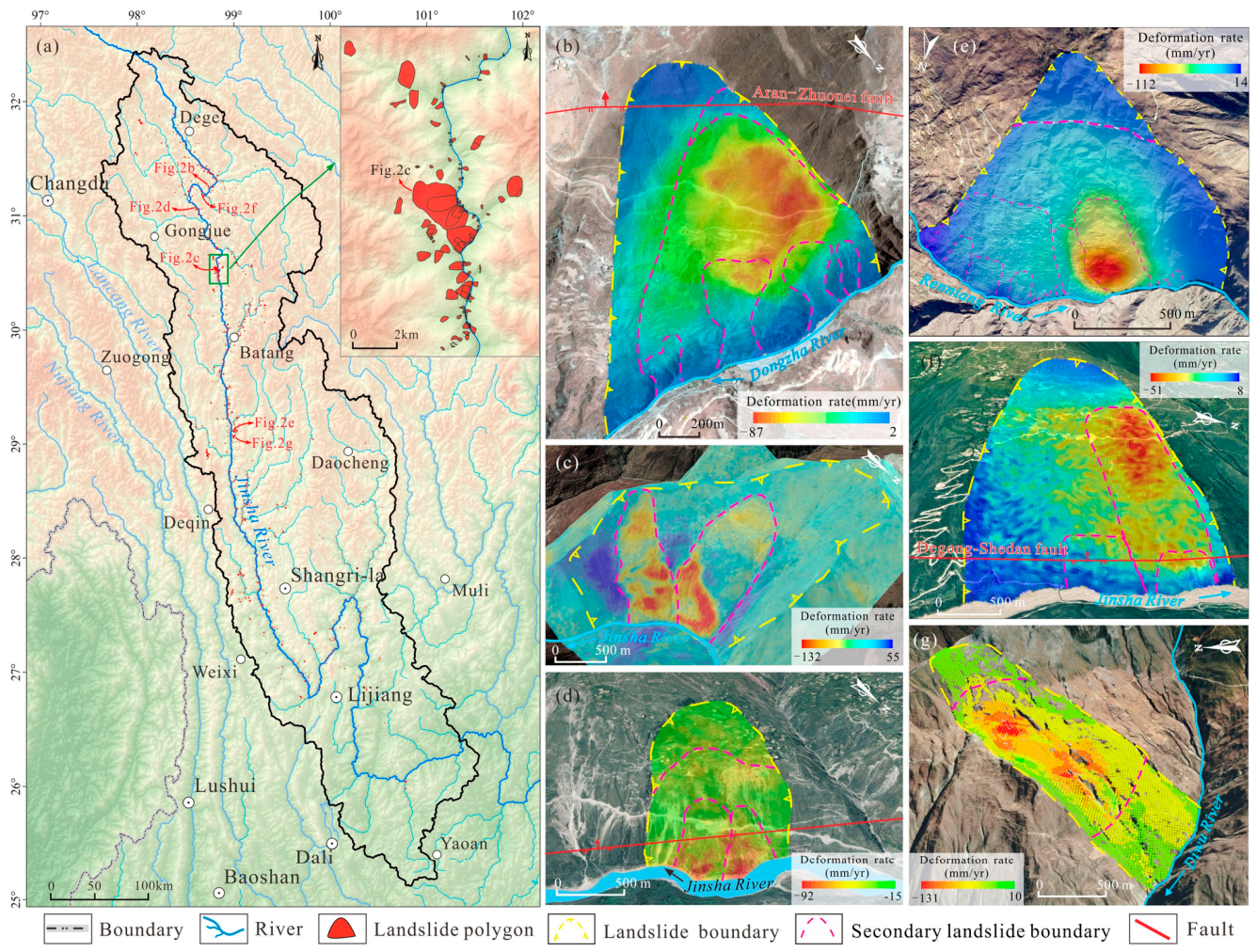
The landslide inventory was compiled based on existing geological hazard investigation datasets collected during 2014–2023 and updated using multi-temporal remote sensing observations. Sentinel-1 InSAR deformation measurements were used to identify active deformation zones and characterize the progressive deformation behavior of unstable slopes. UAV photogrammetry and field investigations conducted during July to August 2022 were performed for representative landslides, including the Tange, Shadingmai, Guili, Xiongba, and Gonghuo landslides to validate the interpreted boundaries and deformation characteristics to validate the interpreted boundaries and deformation features. The identification and delineation of landslide boundaries were based on geomorphological indicators, including main scarp, tension cracks, accumulation zones and persistent surface deformation zones.

By integrating county-level geological hazard datasets, remote sensing interpretation, InSAR observations, UAV validation, and field investigation results, a polygon-based landslide inventory containing 3831 mapped landslide polygons was established (Figure 2a). Unlike conventional point-based inventories, the polygon representation preserves the complete spatial extent, geometric characteristics, and internal structural features of landslides, including source areas, accumulation zones, and secondary deformation zones.

Data Sources and Types

Landslide susceptibility assessment generally requires integrating multi-source datasets, including topography, geological structures, lithology, seismic activity, and precipitation, to characterize the environmental, geological, and climatic conditions of the study area. The main datasets used in this study are as follows:

• Remote sensing imagery: High-resolution satellite images, including Landsat (available at https://earthexplorer.usgs.gov accessed on 14 June 2023), Sentinel-2 (available at https://scihub.copernicus.eu accessed on 18 June 2023), and Planet imagery (available at https://www.planet.com accessed on 1 June 2023), together with UAV aerial photographs, were used for landslide identification. The UAV photogrammetry campaign was carried out in August 2022 using a D20 drone, yielding DSM data with a spatial resolution of approximately 0.2 m/pixel.
• Digital Elevation Model (DEM): The ALOS 12.5 m DEM, downloaded from the Alaska Satellite Facility (https://search.asf.alaska.edu accessed on 21 August 2023), was employed to provide detailed topographic information. It was used to derive elevation, slope, aspect, terrain relief, and river networks, enabling the evaluation of the relationship between landslide occurrence and river proximity.
• Geological maps: The 1:250,000 regional geological map provided by the China Geological Survey (available at http://geocloud.cgs.gov.cn accessed on 12 November 2022) was used to extract lithological information, fault distributions, and geological structural characteristics for engineering geological analysis.
• Active faults and seismic data: Active fault datasets were obtained from the China Earthquake Administration (available at https://www.activefault-datacenter.cn accessed on 12 November 2022) and field investigations, and were used to calculate fault distance. PGA data were obtained from the Fifth-Generation Seismic Zoning Map of China (GB18306-2015, available at http://www.gb18306.net/ accessed on 12 November 2022) to characterize seismic inertial forces that may trigger surface deformation and landslide occurrence.
• Climatic data: Annual mean precipitation data from 2018 to 2022 with a spatial resolution of 30 m × 30 m were obtained from the Resource and Environment Science Data Platform (https://www.resdc.cn accessed on 12 December 2022) and used to characterize regional rainfall conditions.
• Vegetation coverage: The Normalized Difference Vegetation Index (NDVI) was derived from Sentinel-2 remote sensing imagery acquired in 2023 through the Google Earth Engine (GEE) platform (https://www.resdc.cn accessed on 12 December 2022). The NDVI dataset has a spatial resolution of 10 m × 10 m and was calculated using the red (B4) and near-infrared (B8) bands of Sentinel-2 imagery. The NDVI value was used to characterize the vegetation coverage and surface ecological conditions of the study area. In this study, the NDVI dataset represents a single-period vegetation condition indicator and was considered a static environmental conditioning factor in the landslide susceptibility assessment.

Before landslide susceptibility modeling, all multi-source datasets were harmonized to ensure spatial consistency. All raster and vector datasets were transformed into the same coordinate reference system (CGCS2000_3_Degree_GK_CM_99E) and resampled into a unified 30 m × 30 m grid system. Continuous variables, including elevation, precipitation, NDVI, and InSAR-derived deformation rates, were resampled using bilinear interpolation, whereas categorical variables, such as engineering geological rock groups, were processed using the nearest-neighbor method to preserve their original characteristics. The polygon-based landslide inventory was subsequently rasterized according to the same grid system, and all conditioning factors were integrated into a consistent spatial database for model calculations.

3.2. InSAR Deformation Monitoring-Informed Landslide Susceptibility Assessment Framework

Large landslide deformation before failure is jointly controlled by tectonic activity, fluvial incision, rainfall infiltration, and slope unloading. Susceptibility assessment frameworks that only rely on static environmental variables, such as topography, lithology, and fault distribution, are often insufficient for accurately characterizing landslide activity and potential instability.

InSAR technology has been widely applied to landslide detection and surface deformation monitoring [26]. Persistent surface deformation effectively reflects internal stress adjustment and progressive deformation within slopes and can therefore serve as a valuable indicator of landslide activity. Particularly in regions such as the upper Jinsha River, where creeping landslides are extensively developed, continuous deformation information provides important insights into the spatial distribution of potentially active landslides and deep-seated deformation zones.

3.2.1. SAR Datasets and Data Preprocessing

The Sentinel-1A satellite, operated by the European Space Agency (ESA), is equipped with a C-band synthetic aperture radar with a wavelength of 5.6 cm, VV + VH dual polarization mode, and IW imaging mode, and offers a resolution of 5 × 20 m [27,28]. A total of 764 ascending and 876 descending orbit Sentinel-1A images were gathered for the study area, covering the period from November 2014 to October 2023 (

Table 1. The basic parameters of SAR data.

Parameters	Sentinel-1A
Direction	Ascending	Descending
Path	99	33, 135
Frame	1285, 1280, 1275, 1270	487, 492, 497, 498, 502, 503, 508
Band	C	C
Radar wavelength (cm)	5.6	5.6
Incident angle (°)	36.9	38.7
Image interval (days)	12	12
Time	5 November 2014 to 1 October 2023	24 November 2014 to 8 October 2023
Number of images	764	876

).

3.2.2. SBAS-InSAR Method

The Small Baseline Subset InSAR (SBAS-InSAR) method utilizes multi-temporal radar data to monitor ground surface deformation, offering high spatial resolution and low noise interference [29]. This method reconstructs deformation time series by leveraging the spatial coherence of radar targets and connecting multiple interferometric pairs constrained by short temporal and spatial baselines. The SBAS-InSAR data processing sequence comprised the following steps:

• SAR Data Co-registration Process. The initial SAR image was designated as the master image, with the ascending orbit dated 5 November 2014, and the descending orbit dated 24 November 2014. Subsequent auxiliary images were registered against this master image. Using conventional intensity cross-correlation for range co-registration, ensuring a registration accuracy of 1/1000 of a pixel [30].
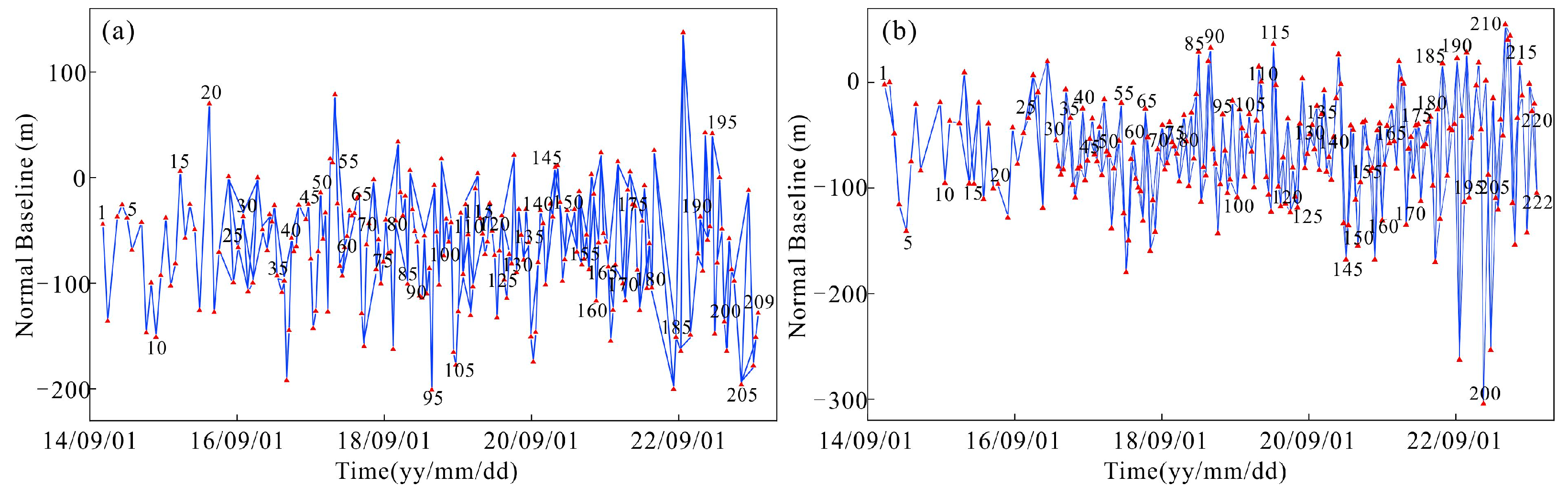
• Differential Interferogram Generation. A multi-look factor of 10:2 was applied to suppress noise and enhance coherence. Interferometric pairs were selected under constraints of a 48-day temporal baseline and a 300-m spatial baseline. After data interferometric processing, and excluding interferograms with poor coherence, a total of 416 high-quality interferograms were obtained from the ascending orbit, and 428 from the descending orbit (Figure 3).

• Phase Filtering and Unwrapping. An adaptive filtering algorithm was applied to reduce phase noise while preserving geophysical signals. Minimum Cost Flow (MCF) was employed for phase unwrapping to resolve integer ambiguities in the filtered interferograms.
• Deformation Parameter Inversion. Atmospheric phase delays were mitigated through spatial filtering and temporal high-pass filtering. High-coherence distributed scatterers were identified and used to derive deformation time series and velocity fields via Singular Value Decomposition (SVD). This process allows the integration of phase velocities from each period in the time domain to obtain the deformation time series for the entire observation period. The reliability of the derived deformation measurements was evaluated through coherence-based quality control and deformation time series stability analysis. Pixels with insufficient coherence were excluded to reduce the influence of decorrelation noise. Furthermore, the uncertainty of deformation measurements was assessed by calculating the standard deviation of deformation time series in stable areas without obvious deformation signals. Only deformation results with reliable quality were retained and subsequently incorporated as a dynamic conditioning factor in the landslide susceptibility model.

In this study, InSAR-derived surface deformation information was not only used to identify active landslide deformation zones but also quantitatively incorporated into the susceptibility model as a dynamic conditioning factor. The deformation rate was calculated from Sentinel-1 InSAR observations and assigned to each sampling unit, enabling the susceptibility assessment model to capture the influence of ongoing slope deformation on landslide occurrence. By introducing dynamic indicators of persistent slope activity alongside conventional static environmental variables, the framework improves the capability of landslide susceptibility assessment in high-relief mountainous regions.

3.3. FR and OFR Models

The FR model is a statistical approach that quantifies the spatial relationship between historical landslide occurrences and environmental conditioning factors and has been widely used in regional landslide susceptibility assessment [31]. The method evaluates the relative contribution of each conditioning factor by calculating the ratio between the probability of landslide occurrence within a specific factor interval and the average probability across the entire study area [32,33]. However, continuous environmental variables need to be discretized into predefined intervals before analysis. Different classification schemes may introduce substantial subjectivity and discontinuities into the calculated frequency ratios, particularly in geomorphologically complex high-relief regions, thereby reducing the sensitivity of the model to environmental variability. The FR model captures the statistical correlation between factor classes and landslide frequency, but cannot reflect nonlinear interactions between factors [34,35].

The Landslide Susceptibility Index (LSI) derived from the FR model is calculated as follows [34] (Equations (1) and (2)):

$$F{R}_j={\displaystyle \frac{A_j/A}{B_j/B}}$$

(1)

$$LSI={\displaystyle \sum _{i=1}^m}{FR}_{ij}$$

(2)

where A_j is the number of grid cells containing landslides within the j interval of a conditioning factor; A is the total number of landslide grid cells in the study area; B_j is the total number of grid cells within the j interval of the conditioning factor; and B is the total number of grid cells in the study area.

To reduce the uncertainty associated with conventional discretization schemes, this study adopted the OFR model proposed by Li et al. [16]. Unlike the conventional FR model, the OFR model calculates frequency ratios based on normalized continuous factor values. The calculation is controlled by only two unified parameters, namely precision and bin width, thereby improving the continuity and stability of FR estimation. By preserving the continuous response characteristics of the environmental variables, the OFR model minimizes the influence of artificial discretization and better characterizes the continuous relationships between conditioning factors and landslide occurrence. The OFR model could provide smoother and more explainable statistical weights; however, it cannot sufficiently characterize nonlinear interactions of complex topographic factors when applied separately [15,16].

The OFR weight and susceptibility index are calculated as follows [16]:

$${OFR}_{i,j}={\displaystyle \frac{P\left(L\right|F_{i,j})}{P\left(L\right|F_i)}}$$

(3)

$${LSI}_{OFR}={\displaystyle \sum _{i=1}^n}{OFR}_{i,j}$$

(4)

where P(L|F_i,j) represents the conditional probability of landslide occurrence within the j interval of factor i, and P(L|F_i) denotes the overall probability of landslide occurrence associated with factor i.

3.4. RF-FR Model and RF-OFR Model

Landslide occurrence in high-relief mountainous regions is controlled by multiple environmental factors exhibiting complex nonlinear interactions. Conventional statistical models often have limited capability to capture these nonlinear relationships among multidimensional variables.

The RF model is a representative ensemble learning algorithm that improves model stability and generalization by integrating a large number of decision trees [36]. Each decision tree in RF is constructed using the Classification and Regression Tree (CART) algorithm, in which the optimal split at each node is selected according to the Gini impurity criterion [37]. The Gini index measures the probability of incorrectly classifying a randomly selected sample if it were labeled according to the class distribution within the node. Therefore, a smaller Gini value indicates a purer node with better class separation. Owing to its computational efficiency, robustness, and effectiveness in handling nonlinear classification problems, the Gini impurity criterion has been widely adopted as the default splitting rule in RF classification models [36]. Assuming that dataset t contains records belonging to n classes, the Gini index is calculated as:

$$Gini\left(t\right)=1-{\displaystyle \sum _{j=1}^n}{p}_j^2$$

(5)

where Gini(t) represents the impurity of dataset t, and P_j denotes the proportion of samples belonging to category j.

Feature importance is evaluated according to the reduction in node impurity achieved by each split. Variables producing larger decreases in Gini impurity contribute more to classification and are therefore assigned higher importance scores. The normalized importance weight of each conditioning factor is calculated as [38]:

$$W_j={\displaystyle \frac{∆j}{{\displaystyle \sum _{j=1}^k}∆j}}$$

(6)

where k is the total number of conditioning factors, Δ_j is the average decrease in the Gini impurity contributed by factor j across all trees, and W_j is the normalized importance weight of the j factor, satisfying:

$${\displaystyle \sum _{j=1}^k}{W}_j=1$$

(7)

To further improve susceptibility assessment performance, coupled RF-FR and RF-OFR models were developed by incorporating RF-derived factor weights into the FR and OFR frameworks, respectively. The RF-FR model could strengthen nonlinear simulation by coupling FR with RF, yet it makes inadequate use of optimized FR weighting information and suffers from low computational efficiency over extensive high-relief terrain [39,40]. The RF-OFR model developed in this research embeds optimized frequency ratios into random forest. It jointly accounts for statistical weights and nonlinear factor interactions to produce robust, interpretable susceptibility outputs. The calculation formula is as follows (Equations (8) and (9)):

$${LSI}_{RF-FR}={\displaystyle \sum _{i=1}^n}{W}_i{FR}_{ij}$$

(8)

$${LSI}_{RF-OFR}={\displaystyle \sum _{i=1}^n}{W}_i{OFR}_{ij}$$

(9)

where W_i is the RF-derived importance weight of conditioning factor i, and FR_ij and OFR_ij represent the FR and OFR values of factor i within interval j, respectively, and n represents the total number of conditioning factors.

3.5. Multi-Scale Polygon-Based Sampling Strategy

The spatial representation of landslide samples exerts a critical influence on landslide susceptibility assessment results. Most regional-scale studies currently employ either point-based sampling or fixed-grid raster sampling strategies. Point-based approaches represent each landslide with the use of a single pixel or centroid, thereby reducing computational cost but inevitably neglecting the pronounced internal spatial heterogeneity of large landslides. Fixed-grid raster approaches preserve spatial completeness by sampling all pixels within landslide polygons. However, they may introduce scale-mismatch problems and spatial bias in complex mountainous environments [41].

In regions such as the upper Jinsha River, where landslides exhibit substantial variability in size, boundary complexity, and internal deformation characteristics, a single sampling resolution cannot adequately represent the full spectrum of landslide spatial heterogeneity. Coarse resolutions may oversimplify large landslide geometries, whereas excessively fine resolutions can introduce redundant information and significantly increase computational cost. Consequently, conventional single-scale sampling approaches are insufficient for accurately characterizing landslide spatial variability in high-relief mountainous regions.

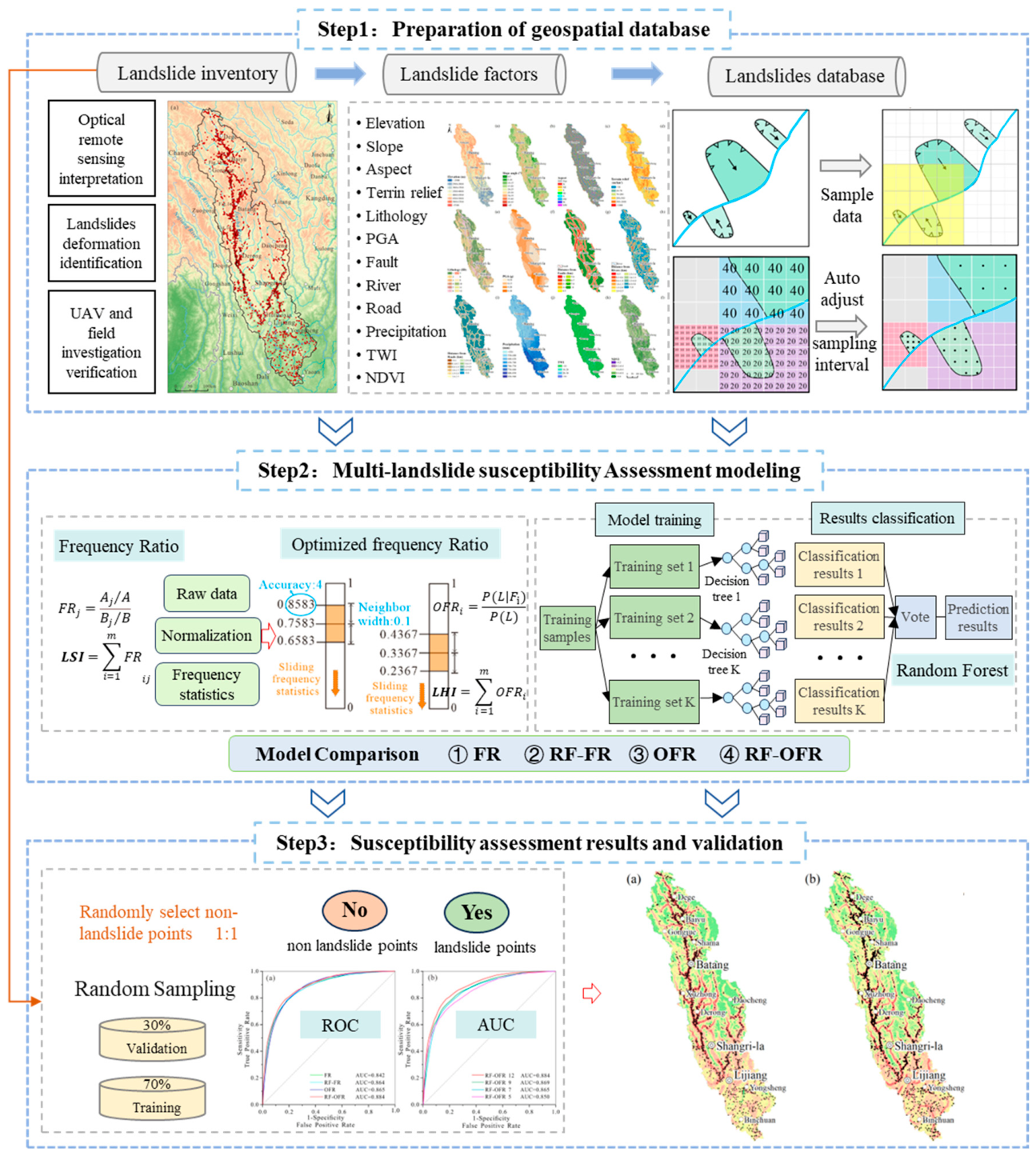
To address this limitation, a multi-scale polygon-based sampling strategy was developed. The method dynamically adjusts sampling resolution according to landslide area by assigning different spatial resolutions to landslides of different sizes (Figure 4). It retains the boundary and internal spatial heterogeneity details of small landslides using fine sampling grids, and simplifies redundant pixel information of large landslides using coarse grids, to balance spatial representativeness and computational efficiency of landslide samples. The whole generation workflow is detailed as follows:

• Through integrated interpretation of optical images, Sentinel-1 InSAR deformation results and field geological surveys, this study established a complete polygon landslide inventory containing 3831 landslides where each independent landslide is enclosed by a closed vector polygon to fully record its real boundary and coverage range.

2.

All landslide polygons were classified of varying sizes based on landslide area thresholds. The corresponding sampling grid resolution allocated to each group is presented in

Table 2. The classification of landslide size and corresponding sampling-grid resolution used in the multi-scale areal sampling strategy.

Scale	Class (n)	Minimum Area (m2)	Grid Size (m)	Number of Landslides
Small	1	<1000	10	291
Medium	2	1000–10,000	20	1051
	3	10,000–100,000	40	1442
	4	100,000–500,000	80	759
Large	5	500,000–1,000,000	160	179
	6	1,000,000–10,000,000	320	109

, and the classification criteria refer to the research of McColl and Cook [42].

3.

Regular raster sampling grids matching the designated resolution were generated inside each landslide polygon, and all grid pixels falling within the polygon boundary were extracted as raster landslide samples.

4.

All sampling pixels derived from landslide polygons of distinct sizes were combined to construct the multi-scale landslide sample dataset. The corresponding environmental factor values were extracted from each sampling unit and used as input variables for subsequent RF-OFR modeling, enabling the model to capture the spatial heterogeneity of large landslides across different scales.

3.6. Model Training and Validation

To develop the regional landslide susceptibility assessment models, both landslide and non-landslide samples were used to construct the modeling dataset. Based on the 74,212 landslide samples, potential non-landslide areas were first identified by excluding mapped landslide polygons, areas within 1000 m buffers around mapped landslides, and persistent InSAR deformation zones. This spatial exclusion strategy was applied to reduce the possibility of including potentially unstable locations in the negative class and minimize negative-class contamination. The spatial distribution of the generated non-landslide samples was further checked against the existing landslide inventory and InSAR deformation results to ensure that they were located in relatively stable areas. Subsequently, an equal number of non-landslide samples were randomly selected from the remaining areas, resulting in a balanced dataset comprising 148,424 samples.

The balanced dataset was randomly partitioned into training and validation subsets at the pixel level with a 70:30 split ratio, where 70% of samples were used for model training and the remaining 30% for independent validation. RF model parameters were optimized using out-of-bag (OOB) error estimation. The number of decision trees was set to 500, while the number of variables considered at each split was set to three [43]. Model performance was evaluated using Receiver Operating Characteristic (ROC) curves and corresponding AUC values, allowing quantitative comparison of the predictive capabilities of the different susceptibility assessment models.

4. Results Analysis

4.1. Conditioning-Factor Analysis of Landslide Occurrence

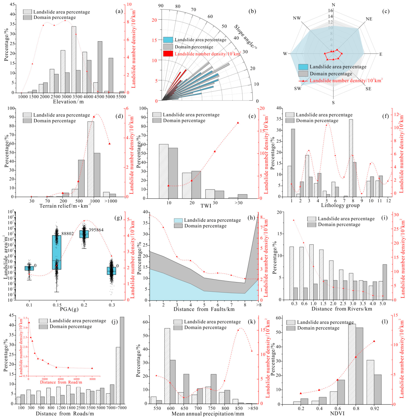
Landslide occurrence in the upper Jinsha River is controlled by the combined effects of topographic, geological, tectonic, climatic, hydrological, and anthropogenic factors. To quantify the relationships between landslide occurrence and environmental conditions, the Landslide Area Percentage (LAP) and Landslide Number Density (LND) were calculated for each factor class. LAP represents the proportion of total landslide area within a given factor interval, whereas LND describes the density of landslides per unit area, and the results are presented in Figure 5 and Figure 6.

4.1.1. Topographic and Geomorphic Factors

The statistical results indicate that 86.28% of landslides occur at elevations of between 2000 and 4000 m, with the highest LND within the 2000~3000 m elevation range (Figure 5a). This elevation interval corresponds to deeply incised valleys with strong relief and active slope adjustment, providing favorable conditions for large-landslide development.

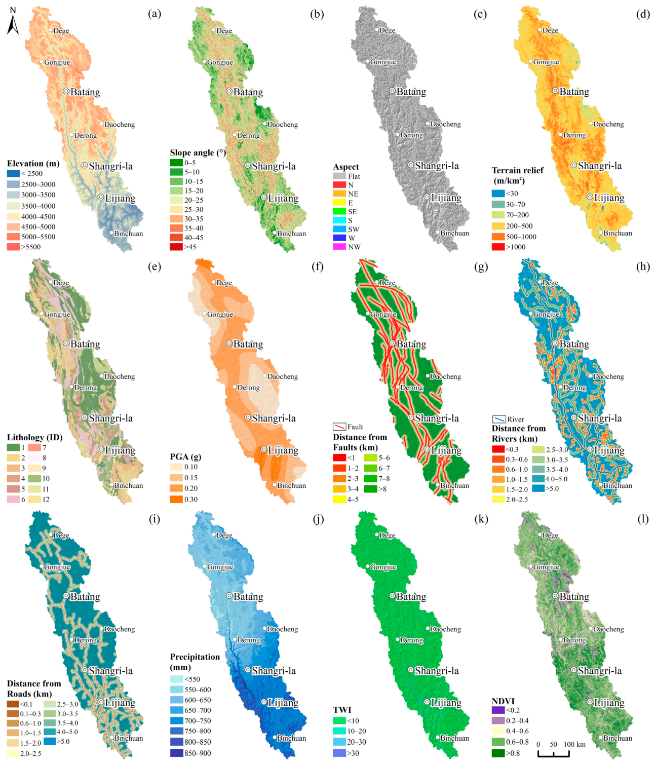
Figure 5. The Spatial distribution of landslide conditioning factors in the upper Jinsha River. (a) Elevation distribution map; (b) Slope angle distribution map; (c) Aspect distribution map; (d) Terrain relief distribution map; (e) Engineering geological lithology distribution map (the descriptions of lithological group ID are provided in Table 3); (f) PGA distribution map; (g) Distance from faults distribution map; (h) Distance from rivers distribution map; (i) Distance from roads distribution map; (j) Mean annual precipitation distribution map; (k) TWI distribution map; (l) NDVI distribution map.

Figure 5. The Spatial distribution of landslide conditioning factors in the upper Jinsha River. (a) Elevation distribution map; (b) Slope angle distribution map; (c) Aspect distribution map; (d) Terrain relief distribution map; (e) Engineering geological lithology distribution map (the descriptions of lithological group ID are provided in Table 3); (f) PGA distribution map; (g) Distance from faults distribution map; (h) Distance from rivers distribution map; (i) Distance from roads distribution map; (j) Mean annual precipitation distribution map; (k) TWI distribution map; (l) NDVI distribution map.

Figure 6. The statistical relationships between landslide and conditioning factors in the upper Jinsha River. (a) Landslide and elevation distribution statistics; (b) Landslide and slope angle distribution statistics; (c) Landslide and aspect distribution statistics; (d) Landslide and terrain relief distribution statistics; (e) Landslide and TWI distribution statistics; (f) Landslide and engineering geological lithology distribution statistics; (g) Landslide and PGA distribution statistics; (h) Landslide and distance from faults distribution statistics; (i) Landslide and distance from rivers distribution statistics; (j) Landslide and distance from roads distribution statistics; (k) Landslide and mean annual precipitation distribution statistics; (l) Landslide and NDVI distribution statistics.

Figure 6. The statistical relationships between landslide and conditioning factors in the upper Jinsha River. (a) Landslide and elevation distribution statistics; (b) Landslide and slope angle distribution statistics; (c) Landslide and aspect distribution statistics; (d) Landslide and terrain relief distribution statistics; (e) Landslide and TWI distribution statistics; (f) Landslide and engineering geological lithology distribution statistics; (g) Landslide and PGA distribution statistics; (h) Landslide and distance from faults distribution statistics; (i) Landslide and distance from rivers distribution statistics; (j) Landslide and distance from roads distribution statistics; (k) Landslide and mean annual precipitation distribution statistics; (l) Landslide and NDVI distribution statistics.

Table 3. Engineering geological lithostratigraphy of Jinsha River.

Lithology ID	Engineering Geological Units	Strata Symbol
1	Hard thick-bedded conglomerate and sandstone rock group	T3l
2	Moderately hard to hard medium- to thick-bedded sandstone interbedded with conglomerate, mudstone, and slate rock group	T3z, P1j
3	Alternating hard and soft medium- to thick-bedded sandstone and mudstone interbedded with limestone, argillaceous limestone, and their interlayers rock group	SDr, T3w, P2, J, C1
4	Weak to moderately hard thin- to medium-thick-bedded sandstone and mudstone with conglomerate–mudstone interbeds rock group	T2–3j
5	Hard medium- to thick-bedded limestone and dolomite rock group	T3g, Sg, P1m
6	Moderately hard thin- to medium-thick-bedded limestone and argillaceous limestone rock group	Dg-t
7	Alternating hard and soft medium- to thick-bedded limestone and dolomite interbedded with sandstone, mudstone, phyllite, and slate rock group	T1–2m
8	Moderately hard to hard thin- to medium-thick-bedded slate, phyllite, and metamorphic sandstone interbedded rock group	D1–2h
9	Weak to moderately hard thin- to medium-thick-bedded phyllite and schist interbedded with limestone, sandstone, and volcanic rocks rock group	T1–2Y, P1e
10	Hard massive basalt-dominated rock group	P2g, T3gl
11	Hard massive granite, andesite, and diorite rock group	Pt2–3N, Pt2, T3MC, Jγδ
12	Soft unconsolidated rock group	Qp, Qh

Table 3. Engineering geological lithostratigraphy of Jinsha River.

Lithology ID	Engineering Geological Units	Strata Symbol
1	Hard thick-bedded conglomerate and sandstone rock group	T3l
2	Moderately hard to hard medium- to thick-bedded sandstone interbedded with conglomerate, mudstone, and slate rock group	T3z, P1j
3	Alternating hard and soft medium- to thick-bedded sandstone and mudstone interbedded with limestone, argillaceous limestone, and their interlayers rock group	SDr, T3w, P2, J, C1
4	Weak to moderately hard thin- to medium-thick-bedded sandstone and mudstone with conglomerate–mudstone interbeds rock group	T2–3j
5	Hard medium- to thick-bedded limestone and dolomite rock group	T3g, Sg, P1m
6	Moderately hard thin- to medium-thick-bedded limestone and argillaceous limestone rock group	Dg-t
7	Alternating hard and soft medium- to thick-bedded limestone and dolomite interbedded with sandstone, mudstone, phyllite, and slate rock group	T1–2m
8	Moderately hard to hard thin- to medium-thick-bedded slate, phyllite, and metamorphic sandstone interbedded rock group	D1–2h
9	Weak to moderately hard thin- to medium-thick-bedded phyllite and schist interbedded with limestone, sandstone, and volcanic rocks rock group	T1–2Y, P1e
10	Hard massive basalt-dominated rock group	P2g, T3gl
11	Hard massive granite, andesite, and diorite rock group	Pt2–3N, Pt2, T3MC, Jγδ
12	Soft unconsolidated rock group	Qp, Qh

Approximately 63% of landslides are distributed on slopes between 20° and 40°. The 25°~40° slope interval exhibits the highest LAP of 48.97% and an LND of 13.15 × 10² km⁻², indicating that moderately steep slopes provide suitable conditions for slope instability (Figure 5b). Extremely gentle slope lack sufficient gravitational driving forces, whereas very steep slopes generally have limited material accumulation.

Landslides are preferentially distributed on E-, SE-, and SW-facing slopes (Figure 5c and Figure 6c). These slope orientations are commonly exposed along river valleys and may experience stronger slope unloading and lateral erosion effects.

Terrain relief shows a strong relationship with landslide occurrence. The highest LAP of 85.23% occurs within the 500~1000 m km⁻² relief range (Figure 5d and Figure 6d), demonstrating that strong relief promotes gravitational deformation and the development of large landslides.

4.1.2. Engineering Geological Lithology

The engineering of the geological lithology exhibits a strong control on landslide distribution. Landslides are mainly concentrated within interbedded weak–strong rock sequences, including sandstone–mudstone–limestone assemblages, and metamorphic rock associations composed of slate, phyllite, and metasandstone (Table 3, Figure 5f). These lithological units commonly contain weak interlayers, discontinuities, and differential weathering zones, which facilitate the formation of potential slip surfaces. Representative large landslides, including the Baige, Temi, and Diwu landslides, are mainly distributed within tectonically fractured zones along the Jinsha River, indicating the combined influence of lithological weakness and structural deformation.

4.1.3. Active Tectonics and Seismicity

Active tectonics and seismic activity show significant relationships with landslide distribution. Landslides are highly concentrated near active fault zones, with LAP reaching 26.78% within 2 km of faults and LND increasing to 15.3 × 10² km⁻² (Figure 6h). Approximately 57.56% of mapped landslides occur within 5 km of fault zones, particularly along the Batang Fault and associated secondary fault (Figure 2).

The decreasing landslide density with increasing distance from faults highlighting the influence of tectonic damage zones on slope instability. In addition, areas with moderate-to-high PGA values exhibit relatively higher landslide density (Figure 6g), suggesting that seismic shaking may further weaken fractured rock masses and promotes slope development.

4.1.4. Fluvial Incision

Landslides exhibit a strong spatial concentration along the Jinsha River and its major tributaries, including the Zengqu, Jiangqu, Baqu, Moqu, and Dingqu Rivers. Within 600 m of river channels, LAP reaches 24.07%, while LND reaches 48.16 × 10² km⁻² (Figure 6i).

The decrease in landslide density with increasing river distance indicates that sustained river incision, lateral erosion and slope toe unloading play important roles in promoting slope instability.

4.1.5. Road Construction Activities

Road construction locally influences landslide occurrence by modifying slope geometry and hydrological conditions through excavation, blasting, and drainage alteration. Where there are slopes within 500 m of roads, the LAP reaches 17.17%, while LND increases to 19.33 × 10² km⁻² (Figure 6j) indicating the relevance of an elevated landslide density in the vicinity of transportation corridors. These results suggest that anthropogenic disturbances can locally enhance slope instability, particularly in areas already characterized by unfavorable geological and geomorphic conditions.

4.1.6. Precipitation and TWI

Precipitation and hydrological conditions exhibit complex relationships with landslide occurrence. The highest LAP occurs within the range of 550~600 mm precipitation rising to a total of 55.61%. However, landslide occurrence does not show a simple increasing trend with precipitation, suggesting that rainfall effects are controlled by multiple factors, including rock mass fracturing, permeability, and groundwater responses (Figure 6k).

The positive relationship between TWI and landslide density (Figure 5k) indicates that areas with stronger water convergence and moisture accumulation are more susceptible to landsliding.

4.1.7. Vegetation Cover

Vegetation cover exhibits a nonlinear relationship with landslide distribution. The highest LAP of up to 55.98% occurs within the NDVI range of 0.6~0.8 (Figure 5l and Figure 6l). This pattern is probably a reflection of the combined influence of vegetation distribution, elevation, precipitation and valley environments rather than the result of a direct causal relationship between vegetation cover and landslide occurrence.

Overall, landslide occurrence in the upper Jinsha River results from the combined influences of deeply incised canyon topography, tectonic deformation, weak lithological conditions, precipitation infiltration, and anthropogenic disturbance. The observed spatial relationships between conditioning factor and landslide distribution provide a quantitative basis for subsequent RF-OFR modeling and susceptibility assessment.

4.2. Response Characteristics of Conditioning Factors

4.2.1. Weight Estimation Based on the OFR Model

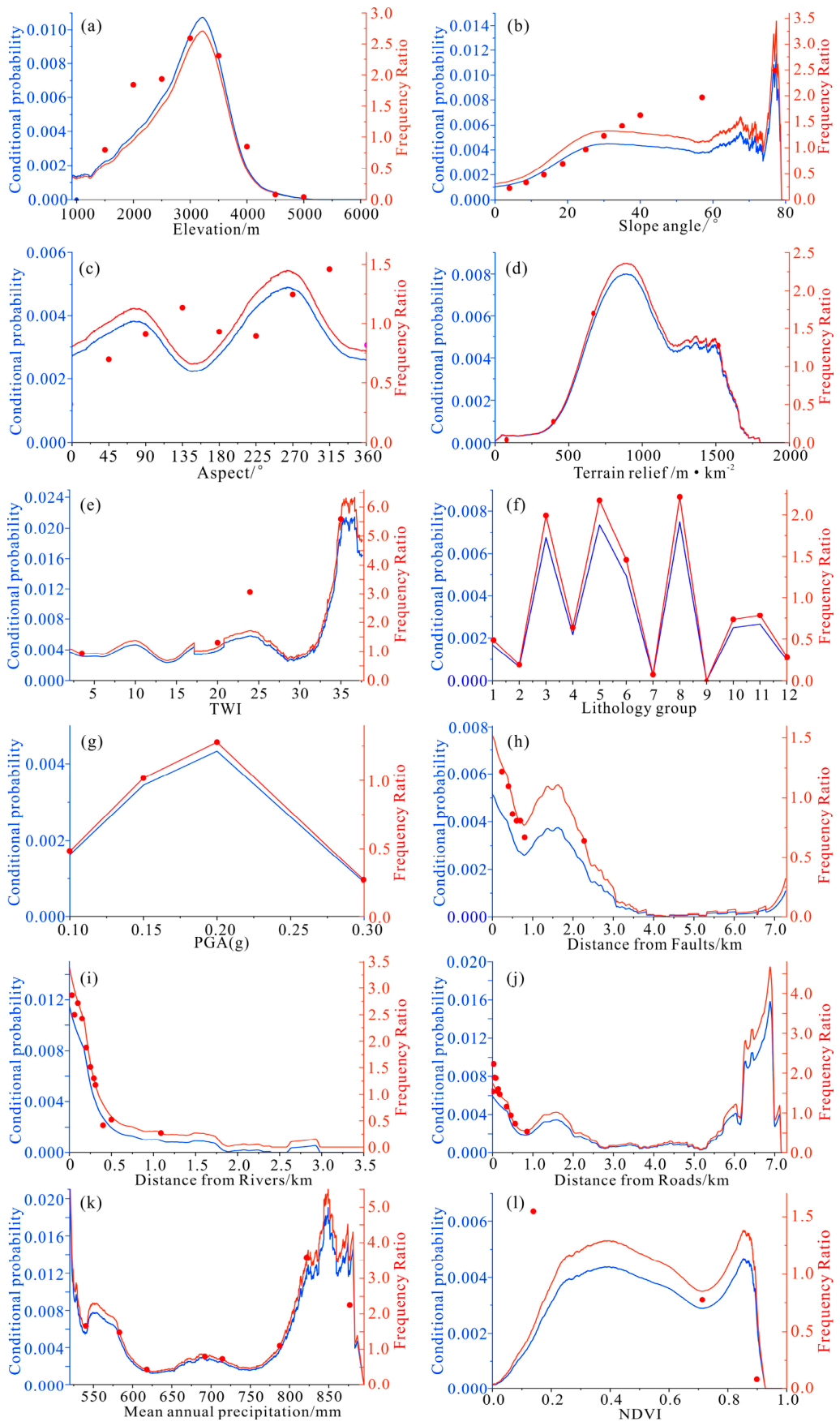
To investigate the response relationships between environmental conditioning factors and landslide occurrence, both the FR and OFR models were applied to the conditioning variables. For discrete variables such as lithology and PGA, the FR method was employed. For continuous variables, including elevation, slope angle, and distance to rivers, the OFR model was additionally applied to achieve continuous representation and reduce the uncertainty associated with subjective classification schemes. The output raster resolution, precision parameter, and neighborhood window width were set to 30 m, 4, and 0.1, respectively. The results demonstrate that the OFR model provides a more continuous and physically meaningful representation of the relationships between environmental variables and landslide occurrence (Figure 7).

Compared with the FR model, the OFR model substantially reduces abrupt fluctuations in frequency ratio values and improves the detection of subtle sensitivity variations among conditioning factors. This advantage is particularly evident in high-relief mountainous regions, where environmental variables such as topography and fluvial incision exhibit strong spatial gradients. Consequently, the OFR-derived response curves are smoother, more stable and better able to capture the continuous response characteristics of landslide occurrence.

4.2.2. Weight Estimation Based on the RF Model

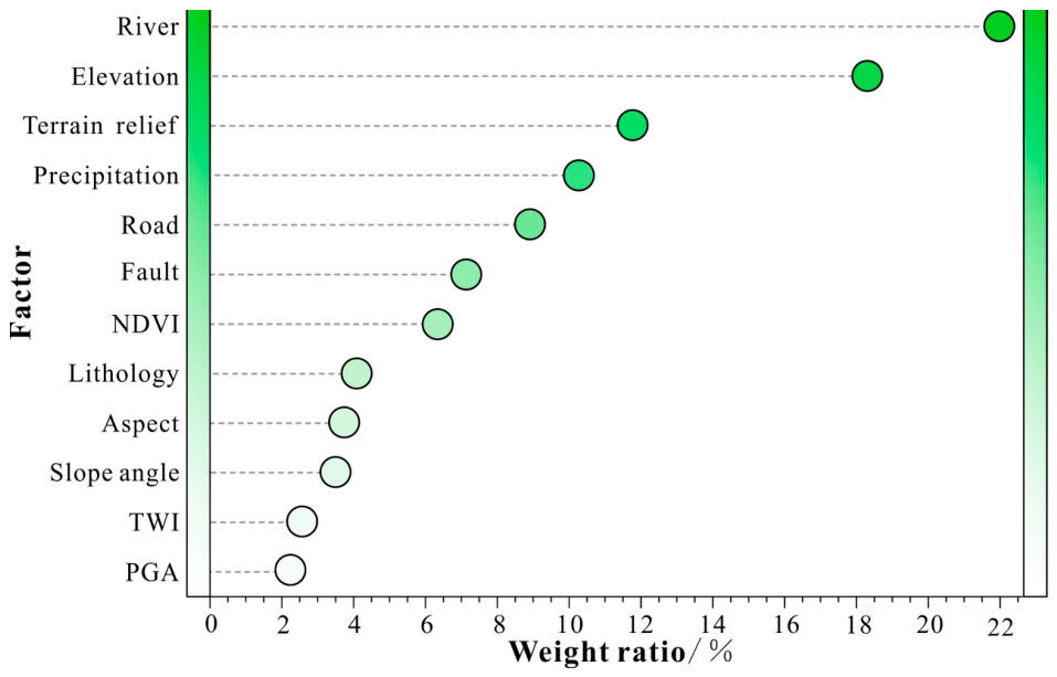
In the RF model, feature importance is quantified according to the contribution of each conditioning factor to impurity across all decision trees in the ensemble. Factors producing greater reductions in node impurity reduction are considered more influential in controlling landslide occurrence [44]. The Mean Decrease Gini results (Figure 8) indicate that distance to rivers, elevation, terrain relief, and mean annual precipitation are the dominant controlling factors governing landslide spatial distribution in the study area. These variables collectively reflect the coupled influences of fluvial incision, topographic differentiation, and climatic forcing on landslide development. In contrast, factors such as aspect and distance to roads exhibit relatively lower importance, suggesting that their effects are secondary and largely dependent on interactions with other environmental variables.

4.3. Model Validation and Predictive Performance

The ROC Curve is a graphical tool used to depict the performance of a classifier. The ROC curve evaluates the model’s ability to distinguish between landslide and non-landslide samples and is widely employed for assessing the performance of landslide susceptibility prediction models [45,46].

In this study, True Positive (TP) refers to the number of landslide pixels correctly identified, while False Positive (FP) refers to non-landslide pixels incorrectly classified as landslides. Similarly, True Negative (TN) denotes the number of correctly identified non-landslide pixels, and False Negative (FN) indicates landslide pixels incorrectly identified as non-landslides. Specificity and sensitivity are calculated using Equations (10) and (11). The AUC quantitatively represents the classification accuracy of the model.

$$Sensitivity={\displaystyle \frac{TP}{TP+FN}}$$

(10)

$$1-Specificity={\displaystyle \frac{FP}{FP+TN}}$$

(11)

The AUC represents the area beneath the ROC curve and is used to evaluate classifier performance, with values ranging from 0 to 1. An AUC value close to 1 indicates excellent model performance, whereas a value near 0.50 suggests poor predictive capability. In general, an AUC greater than 0.70 is considered indicative of high model accuracy [45].

$$AUC={\int }_0^{1}TPR\left(FPR\right)dFPR$$

(12)

where TPR refers to the True Positive Rate, and FPR refers to the False Positive Rate.

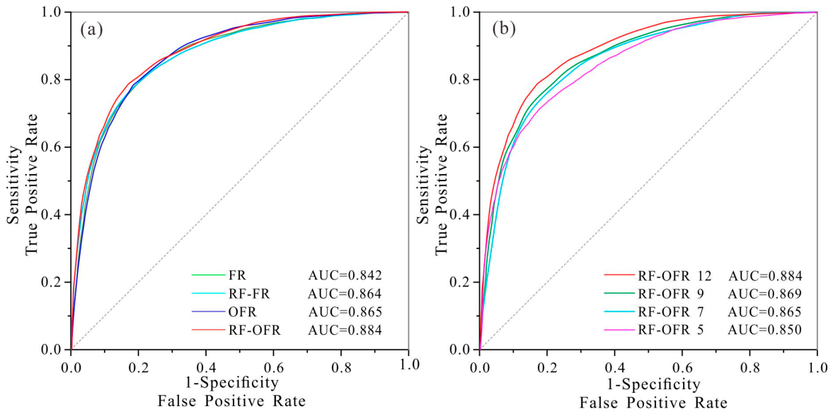
The ROC curves and corresponding AUC values indicate that all evaluated models achieved satisfactory performance in characterizing the spatial distribution of landslides within the study area (Figure 9). The AUC values of the FR, RF-FR, OFR, and RF-OFR models are 0.846, 0.864, 0.879, and 0.906, respectively, demonstrating that the RF-OFR model provides the highest predictive accuracy among all tested approaches.

Compared with the FR model, the RF-OFR framework more effectively captures the complex nonlinear interactions among environmental conditioning factors in the high-relief mountainous regions while reducing information loss associated with the discretization of continuous variables. The OFR component improves the continuous representation of environmental responses and preserves the intrinsic relationships between conditioning factors and landslide occurrence. Meanwhile, the RF component enhances the model’s ability to identify multidimensional nonlinear coupling effects and quantify the relative importance of conditioning factors. Consequently, the integrated RF-OFR model exhibits superior predictive capability under complex mountainous terrain conditions.

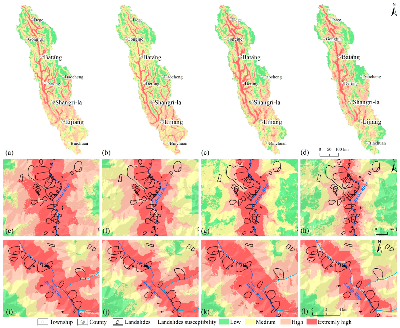
Furthermore, susceptibility maps generated by the RF-OFR model reveal a distinct belt-like zone of high susceptibility distributed along the main Jinsha River corridor and its major tributaries. These spatial patterns closely correspond to the observed distribution of large landslides and InSAR-derived surface deformation zones, highlighting the importance of long-term deformation processes in controlling landslide evolution and spatial occurrence.

4.4. Spatial Distribution of Landslide Susceptibility

The continuous landslide susceptibility index generated by the RF-OFR model was classified into four susceptibility levels, including low, medium, high, and extremely high susceptibility, using the Natural Breaks (Jenks optimization) method. The classification thresholds were automatically determined according to the statistical distribution characteristics of susceptibility values by minimizing within-class variance and maximizing between-class variance [47].

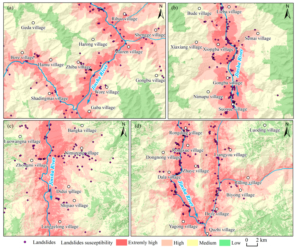
The susceptibility map generated using the RF-OFR model indicates that high and extremely high susceptibility zones are predominantly distributed in elongated belts along the main channel of the Jinsha River and its major tributaries, including the Baqu and Dingqu Rivers (Figure 10 and Figure 11;

Table 4. A comparison of the landslide susceptibility assessment results and the predictive performance of the four models.

Models	Percentage of Susceptibility Areas (%)				AUC
	Extremely High	High	Medium	Low
FR	9.10	29.06	40.4	21.44	0.846
RF-FR	9.56	25.66	45.58	19.20	0.864
OFR	12.76	27.10	37.91	22.23	0.879
RF-OFR	9.65	30.83	32.13	27.39	0.906

). These areas exhibit strong spatial correspondence with active fault systems, zones of intense fluvial incision, and regions characterized by high concentrations of large landslides.

From a regional perspective, the study area can be divided into five major landslide concentration zones: the Jiangda–Baiyu, Xiongba–Sela, Lawa–Suwalong, Zhongxinrong–Diwu, and Derong–Guxue sections (Figure 11). These zones are characterized by deeply incised valleys, dense active fault networks, highly fractured rock masses, and strong fluvial incision. Among them, Baiyu County, Batang County and Derong County exhibit the most extensive and continuous high susceptibility zones. These regions show strong spatial agreement with InSAR-derived deformation patterns and the distribution of large landslides, emphasizing the critical role of long-term deformation processes in landslide development.

• Extremely high and high susceptibility zones: occupy approximately 4.62 × 10⁴ km², accounting for 40.48% of the total study area. These zones are concentrated along the Jinsha River and its major tributaries and are characterized by steep slopes, active tectonic deformation, weak lithological conditions, and relatively high precipitation. Landslide occurrence is particularly concentrated in river valleys and fault damage zones, where multiple conditioning factors interact to promote slope instability.
• Medium susceptibility zones: cover approximately 3.66 × 10⁴ km², representing 32.13% of the study area. These areas are primarily distributed around urbanized regions, including Lijiang, along major transportation corridors, and within transitional zones between mountain ridges and valley bottoms. They are characterized by moderate slope gradients, intermediate relief, and mixed geological conditions.
• Low susceptibility zones: cover approximately 3.12 × 10⁴ km², accounting for 27.39% of the study area. These areas are mainly located in high-elevation regions characterized by relatively gentle terrain, competent bedrock and limited human activity. Consequently, the probability of landslide occurrence is comparatively low.

5. Discussion

5.1. Advantages of the RF–OFR Model for Landslide Susceptibility Assessment in High-Relief Mountainous Regions

To overcome the limitations of conventional statistical approaches, this study developed an RF-OFR susceptibility framework by integrating the RF algorithm with the OFR model. Comparative analyses demonstrate that the RF-OFR model achieves the highest predictive performance among all of the evaluated models, with an AUC value of 0.906. Rather than simply reflecting the superiority of a hybrid algorithm, this improvement suggests that integrating nonlinear machine learning with continuous probabilistic analysis is better suited to representing the complex environmental conditions and spatial heterogeneity of large landslides in high-relief mountainous regions. The superior performance of the RF-OFR model can be attributed to three key advantages:

First, the RF algorithm possesses strong nonlinear learning capabilities and can effectively capture complex interactions among multiple conditioning factors. Through bootstrap resampling and ensemble decision tree construction, RF reduces model variance and mitigates overfitting, thereby enhancing model stability and predictive generalization [48]. This capability is particularly important in the upper Jinsha River, where landslide development results from long-term interactions among the tectonic deformation, river incision, hydrogeological processes, and hydrogeological processes, and climate forcing rather than from any single conditioning factor.

Second, the OFR model addresses a major limitation of the FR approaches by avoiding a subjective discretization of continuous variables. Conventional FR models require environmental variables to be divided into predefined intervals, and the resulting susceptibility estimates can vary substantially depending on the classification scheme adopted. In contrast, the OFR model preserves the continuity of environmental responses and more accurately represents the intrinsic relationships between conditioning factors and landslide occurrence. This characteristic is especially advantageous in the study area because environmental variables often exhibit strong spatial gradients associated with deeply incised valleys and rapid elevation changes.

Third, the integration of RF and OFR combines the nonlinear predictive capability of machine learning with the interpretability and statistical rigor of probabilistic susceptibility analysis. The RF-derived factor weights enable objective quantification of variable importance, while the OFR framework provides continuous response relationships between conditioning factors and landslide occurrence. Consequently, the coupled model can capture both the nonlinear relationships among conditioning factors and the continuous environmental responses that characterize large-landslide development in tectonically active mountainous regions.

From a spatial perspective, the susceptibility patterns generated by the RF-OFR model show strong agreement with the observed distribution of landslides. High-susceptibility zones are predominantly concentrated along the main Jinsha River valley and major tributaries, including the Baqu and Dingqu Rivers. These regions are characterized by steep valley-side slopes, intense fluvial incision, active faulting, highly fractured rock masses, and persistent rainfall infiltration. This strong spatial correspondence suggests that the proposed framework effectively captures the dominant geomorphic and tectonic controls governing regional landslide occurrence, rather than merely improving statistical prediction accuracy.

Importantly, the incorporation of InSAR-derived surface deformation information represents an additional advantage of the proposed framework. Persistent surface deformation serves as a direct indicator of slope activity and reflects ongoing stress adjustment and progressive deformation processes within landslide bodies. By integrating dynamic deformation information with conventional environmental variables, the RF-OFR framework more effectively captures both the preconditioning and evolutionary characteristics of landslide development. This capability is particularly valuable in high-relief mountainous regions, where many large landslides undergo prolonged deformation before catastrophic failure. These findings highlight that incorporating dynamic deformation information complements conventional static conditioning factors and is particularly valuable for identifying large landslides that remain in prolonged stages of progressive deformation.

5.2. Multi-Factor Coupling Mechanisms and Dominant Conditioning Factors

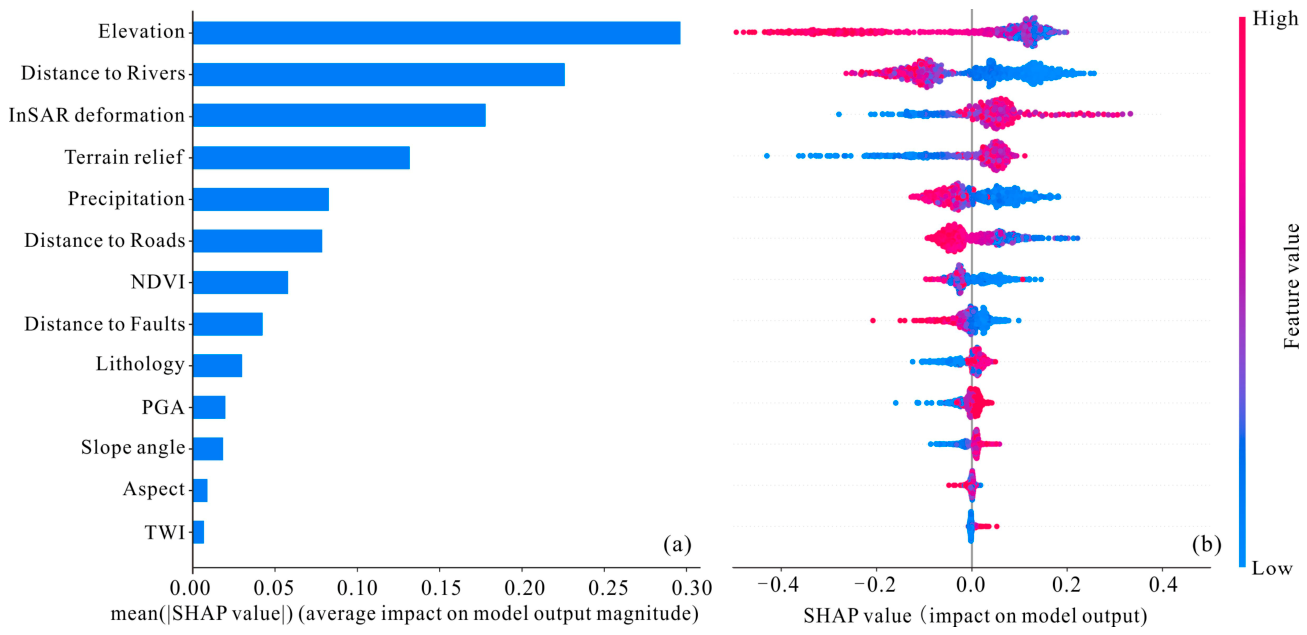
Landslide initiation and evolution are governed by the combined influences of topography, geological structure, hydrological processes, climatic forcing, and human activities. Owing to differences in tectonic setting, geomorphic evolution, and external driving forces, the dominant controls on landslide occurrence vary considerably among regions [10]. To further elucidate the mechanisms controlling landslide development in the upper Jinsha River, Shapley Additive Explanations (SHAP) analysis was applied to interpret the RF-OFR model and quantify both the relative importance and directional influence of individual conditioning factors. Positive SHAP values indicate a positive contribution to landslide occurrence, Class 1, whereas negative values indicate a contribution toward non-landslide conditions, Class 0.

The SHAP results reveal that distance to rivers, elevation, terrain relief, and mean annual precipitation are the most influential factors controlling landslide occurrence in the study area. Among these variables, distance to rivers exhibits the highest contribution, highlighting the dominant role of fluvial incision in landslide development. Locations closer to river channels are generally associated with positive SHAP values, whereas increasing distance from rivers corresponds to progressively lower susceptibility. This pattern reflects the long-term effects of river incision and lateral erosion, which continuously remove slope support, induce stress redistribution, and promote deep-seated gravitational deformation and traction-induced landslides [49]. The widespread concentration of large landslides along deeply incised valleys throughout the study area provides further evidence for the critical geomorphic control exerted by fluvial erosion (Figure 12).

Elevation and terrain relief also exhibit strong explanatory power. Low- to mid-elevation zones are generally associated with positive SHAP values, whereas high-elevation areas contribute negatively to landslide susceptibility. This pattern is consistent with the geomorphic framework of the upper Jinsha River, where most large landslides are concentrated along deeply incised valley slopes rather than on high-elevation ridge crests. Similarly, increasing terrain relief corresponds to progressively higher susceptibility values, indicating that intense topographic dissection promotes gravitational stress concentration, slope unloading, and long-term deformation. These processes ultimately facilitate progressive failure of deep-seated landslides.

Precipitation represents another critical triggering factor. Areas characterized by higher annual precipitation generally exhibit positive SHAP contributions, indicating that rainfall infiltration promotes landslide deformation by increasing pore water pressure and reducing the shear strength of slope materials. In tectonically fractured rock masses, precipitation-induced infiltration may further accelerate groundwater circulation and amplify instability processes. The combined effects of fractured bedrock, intense relief, and concentrated rainfall therefore create favorable conditions for progressive landslide deformation.

In addition to geomorphic and climatic controls, active tectonics exerts a fundamental influence on landslide occurrence. The SHAP analysis indicates elevated susceptibility values in proximity to active faults, reflecting strong structural control on landslide distribution. The study area is traversed by several major fault systems, including the Jinsha River Fault and Batang Fault. Long-term tectonic activity has generated highly fractured rock masses, pervasive discontinuities, and weakened structural zones, substantially reducing slope integrity. Furthermore, repeated seismic loading promotes crack propagation, stress redistribution, and rock mass degradation, thereby preconditioning slopes for failure under the combined influences of fluvial incision and precipitation. These observations indicate that landslide development in the upper Jinsha River is fundamentally controlled by the long-term coupling of tectonic deformation, river incision, climatic forcing, and progressive slope deformation.

To investigate how conditioning-factor selection affects model performance and eliminate circularity in feature selection, this study conducted factor subsets of 12, 9, 7, and 5 variables on a SHAP importance ranking derived purely from the training dataset (

Table 5. The comparison of susceptibility assessment results obtained using different conditioning-factor combinations within the RF-OFR model.

Num.	Factors	Percentage of Susceptibility Areas (%)				AUC
		Extremely High	High	Medium	Low
5	elevation, distance to rivers, InSAR deformation, terrain relief, mean annual precipitation	9.89	26.87	35.69	27.55	0.862
7	elevation, distance to rivers, InSAR deformation, terrain relief, mean annual precipitation, distance to roads, NDVI	10.87	27.68	36.8	24.65	0.866
9	elevation, distance to rivers, InSAR deformation, terrain relief, mean annual precipitation, distance to roads, NDVI, distance to faults, lithological units	13.48	25.66	35.14	25.72	0.885
12	elevation, distance to rivers, InSAR deformation, terrain relief, mean annual precipitation, distance to roads, NDVI, distance to faults, lithological units, PGA, slope, aspect	9.65	30.83	32.13	27.39	0.906

; Figure 12). Briefly, the RF-OFR model was trained on training samples to compute SHAP values and quantify factor contributions, models corresponding to each factor subset were then trained independently and validated using separate test samples. The model incorporating all conditioning factors achieved the highest predictive accuracy, with an AUC value of 0.906. When only the five most important factors were retained, predictive performance decreased markedly, with the AUC declining to 0.862. Intermediate models containing seven and nine factors gave AUC values of 0.866 and 0.885, respectively.

The SHAP analysis further demonstrates that the relative importance of conditioning factors reflects the regional geomorphic evolution of the upper Jinsha River. In particular, the dominant contribution of distance to rivers emphasizes the critical role of long-term fluvial incision in controlling the spatial distribution of large landslides, whereas tectonic activity and precipitation mainly act by preconditioning slopes and triggering instability. Although the five highest-ranked variables explain the principal regional susceptibility pattern, the remaining conditioning factors provide complementary information that reflects local geological heterogeneity. Variables such as lithology, fault proximity, slope aspect, and land cover help distinguish slopes with similar topographic characteristics but different geological or environmental settings, thereby improving the model’s spatial generalization capability. These findings suggest that factor selection should not rely solely on statistical importance rankings. Instead, both the regional geological setting and the physical mechanisms controlling landslide development should be considered. In complex high-relief mountainous regions, combining dominant regional controls with complementary local factors is more effective than relying exclusively on a limited number of predictors, thereby improving both model robustness and geological interpretability.

It should definitely to noted that increasing the number of conditioning factors does not necessarily guarantee improved model performance. Previous studies have demonstrated that excessive or highly correlated variables may introduce redundancy, increase model complexity, and reduce computational efficiency [7]. Therefore, future susceptibility studies should integrate statistical feature selection techniques with geological knowledge to identify an optimal combination of conditioning factors rather than simply increasing the number of input variables.

6. Conclusions

This study developed a refined landslide susceptibility assessment framework that integrates multi-scale polygon-based sampling and surface deformation constraints and applied it to the upper Jinsha River region on the southeastern Tibetan Plateau. The principal conclusions are as follows:

First, by integrating optical remote sensing, InSAR observations, UAV surveys, and field investigations, a polygon-based landslide inventory containing 3831 landslides was established. The inventory provides a comprehensive dataset for regional landslide susceptibility assessment and supports analyses of landslide spatial characteristics in high-relief mountainous terrain.

Second, landslides are predominantly distributed at elevations of between 2000 and 3500 m and on slopes ranging from 25° to 40°. East-, southeast-, and southwest-facing slopes exhibit the highest landslide densities. Approximately 32.39% of mapped landslides are concentrated along the main Jinsha River corridor, whereas 57.56% occur within active fault-influenced zones, particularly along the Batang Fault and Jinsha River Fault, indicating the combined influence of fluvial incision and tectonic activity on regional landslide distribution.

Third, the proposed multi-scale polygon-based sampling strategy accounts for the substantial variability in landslide size and morphology by adjusting sampling resolution according to landslide area. Compared with conventional point-based sampling, this approach better preserves the spatial characteristics of large landslides, reduces sampling bias, and improves the representativeness of training samples for susceptibility modeling within the study area.

Fourth, among the evaluated models, the RF-OFR model achieved the highest predictive performance, with an AUC value of 0.906, representing improvements of 6.0%, 4.2%, and 2.7% over the FR, RF-FR, and OFR models, respectively. The results suggest that integrating machine learning techniques with continuous probabilistic analysis can improve susceptibility prediction for large landslides under the environmental conditions represented in the study area.

Five, SHAP analysis indicates that distance to rivers, elevation, terrain relief, and mean annual precipitation are the dominant conditioning factors in the upper Jinsha River region. The results suggest that the spatial distribution of large landslides reflects the combined effects of long-term fluvial incision, tectonic deformation, climatic forcing, and progressive slope evolution. Factor-combination experiments further demonstrate that incorporating complementary geological and environmental variables improves susceptibility prediction by better representing regional environmental heterogeneity.

Although the proposed framework achieved satisfactory predictive performance in the upper Jinsha River region, its applicability to other mountainous environments requires further validation because landslide-controlling factors and their relative importance vary among different geological and climatic settings. In addition, the present study relied on a single regional landslide inventory and InSAR deformation dataset. Future studies should evaluate the transferability of the proposed framework in other regions and incorporate additional time-dependent deformation observations and geological information to further improve model robustness and general applicability.

References

1. Cui, P.; Ge, Y.G.; Li, S.J.; Li, Z.H.; Xu, X.W.; Zhou, G.; Chen, H.Y.; Wang, H.; Lei, Y.; Zhou, L.B.; et al. Scientific challenges in disaster risk reduction for the Sichuan-Tibet Railway. Eng. Geol. 2022, 309, 106837. [Google Scholar] [CrossRef] [Scilit]
2. Li, Z.Z.; Chen, J.P.; Cao, C.; Zhang, W.; Li, Y.C.; Hu, J.Y.; Li, Z. Detecting subtle nonlinear changes in slow-moving landslides with a hybrid InSAR change point detection framework: Methodological assessment and validation. Int. J. Appl. Earth Obs. Geoinf. 2025, 144, 104949. [Google Scholar] [CrossRef] [Scilit]
3. Varnes, D.J. Slope Movement Types and Processes. In Landslides, Analysis and Control, Special Report 176; Schuster, R.L., Krizek, R.J., Eds.; Transportation Research Board, National Academy of Sciences: Washington, DC, USA, 1978; pp. 11–33. [Google Scholar]
4. Hungr, O.; Leroueil, S.; Picarelli, L. The Varnes classification of landslide types, an update. Landslides 2014, 11, 167–194. [Google Scholar] [CrossRef] [Scilit]
5. Fan, X.M.; Xu, Q.; Alonso-Rodriguez, A.; Subramanian, S.S.; Li, W.L.; Zheng, G.; Dong, X.J.; Huang, R.Q. Successive landsliding and damming of the Jinsha River in eastern Tibet, China: Prime investigation, early warning, and emergency response. Landslides 2019, 16, 1003–1020. [Google Scholar] [CrossRef] [Scilit]
6. Zhang, Y.S.; Ren, S.S.; Liu, X.Y.; Guo, C.B.; Li, J.Q.; Bi, J.B.; Ran, L.N. Reactivation mechanism of old landslide triggered by coupling of fault creep and water infiltration: A case study from the east Tibetan Plateau. Bull. Eng. Geol. Environ. 2023, 82, 291. [Google Scholar] [CrossRef] [Scilit]
7. Ullah, I.; Aslam, B.; Shah, S.H.I.A.; Tariq, A.; Qin, S.J.; Majeed, M.; Havenith, H. An integrated approach of machine learning, remote sensing, and GIS data for the landslide susceptibility mapping. Land 2022, 11, 1265. [Google Scholar] [CrossRef] [Scilit]
8. Huang, W.B.; Ding, M.T.; Li, Z.H.; Yu, J.C.; Ge, D.Q.; Liu, Q.; Yang, J. Landslide susceptibility mapping and dynamic response along the Sichuan-Tibet transportation corridor using deep learning algorithms. CATENA 2023, 222, 106866. [Google Scholar] [CrossRef] [Scilit]
9. Myronidis, D.; Papageorgiou, C.; Theophanous, S. Landslide susceptibility mapping based on landslide history and analytic hierarchy process (AHP). Nat. Hazards 2016, 81, 245–263. [Google Scholar] [CrossRef] [Scilit]
10. Guo, C.B.; Montgomery, D.R.; Zhang, Y.S.; Wang, K.; Yang, Z.H. Quantitative assessment of landslide susceptibility along the Xianshuihe fault zone, Tibetan Plateau, China. Geomorphology 2015, 248, 93–110. [Google Scholar] [CrossRef] [Scilit]
11. Pradhan, A.M.S.; Kim, Y.T. Evaluation of a combined spatial multi-criteria evaluation model and deterministic model for landslide susceptibility mapping. CATENA 2016, 140, 125–139. [Google Scholar] [CrossRef] [Scilit]
12. Regmi, N.R.; Giardino, J.R.; Vitek, J.D. Modeling susceptibility to landslides using the weight of evidence approach: Western Colorado, USA. Geomorphology 2010, 115, 172–187. [Google Scholar] [CrossRef] [Scilit]
13. Huang, Y.; Zhao, L. Review on landslide susceptibility mapping using support vector machines. CATENA 2018, 165, 520–529. [Google Scholar] [CrossRef] [Scilit]
14. Hussain, M.A.; Chen, Z.; Zhou, Y.; Meena, S.R.; Ali, N.; Shah, S.U. Landslide susceptibility mapping using artificial intelligence models: A case study in the Himalayas. Landslides 2005, 22, 2089–2103. [Google Scholar] [CrossRef] [Scilit]
15. Li, L.P.; Lan, H.X.; Guo, C.B.; Zhang, Y.S.; Li, Q.W.; Wu, Y.M. A modified frequency ratio method for landslide susceptibility assessment. Landslides 2017, 14, 727–741. [Google Scholar] [CrossRef] [Scilit]
16. Li, L.P.; Lan, H.X. Bivariate landslide susceptibility analysis: Clarification, optimization, open software, and preliminary comparison. Remote Sens. 2023, 15, 1418. [Google Scholar] [CrossRef] [Scilit]
17. Liu, X.J.; Zhao, C.Y.; Zhang, Q.; Lu, Z.; Li, Z.H.; Yang, C.S.; Zhu, W.; Liu-Zeng, J.; Chen, L.Q.; Liu, C.J. Integration of Sentinel-1 and ALOS/PALSAR-2 SAR datasets for mapping active landslides along the Jinsha River corridor, China. Eng. Geol. 2021, 284, 106033. [Google Scholar] [CrossRef] [Scilit]
18. Zhou, J.W.; Xu, W.Y.; Yang, X.G.; Shi, C.; Yang, Z.H. The 28 October 1996 landslide and analysis of the stability of the current Huashiban slope at the Liangjiaren Hydropower Station, Southwest China. Eng. Geol. 2010, 114, 45–56. [Google Scholar] [CrossRef] [Scilit]
19. Yan, Y.Q.; Guo, C.B.; Qiu, Z.D.; Li, C.H.; Liu, G.; Yuan, H.; Pudasaini, S.P. Types and mechanism of deep-seated gravitational-deformation slopes in tectonics active zone: A high-resolution study of the Diwu landslide along the Jinsha River Fault Zone, Tibetan Plateau. Landslides 2026, 23, 159–178. [Google Scholar] [CrossRef] [Scilit]
20. Chang, H.; Chang, Z.F.; Liu, C.W. The relationship between activity of Jinsha River fault zone and large-scale landslides: A case study of the section between Narong and Rongxue along the Jinsha River. Seismol. Geol. 2021, 43, 1435–1458, (In Chinese with English). [Google Scholar]
21. Zhou, H.F.; Wang, M.; Xue, J.Y.; Li, R.; Hu, J.P.; Xing, J.; Fang, T. Slide-controlling modes and classification system of the mélange high slopes: Insight into a disaster-causing mechanism of the Jinsha River mélange belt in the eastern Tibetan Plateau. Bull. Eng. Geol. Environ. 2024, 83, 328. [Google Scholar] [CrossRef] [Scilit]
22. Li, Y.C.; Chen, J.P.; Li, Z.H.; Han, X.D.; Zhai, S.J.; Li, Y.C.; Zhang, Y.W.; Gu, F.F. Comprehensive analysis of a paleo-landslide damming event on the upper reach of the Jinsha River, SE Tibetan Plateau. Bull. Eng. Geol. Environ. 2022, 81, 334. [Google Scholar] [CrossRef] [Scilit]
23. Guo, C.B.; Yan, Y.Q.; Zhang, Y.S.; Zhang, X.J.; Zheng, Y.Z.; Li, X.; Yang, Z.H.; Wu, R.A. Study on the creep-sliding mechanism of the giant Xiongba ancient landslide based on the SBAS-InSAR method, Tibetan Plateau, China. Remote Sens. 2021, 13, 3365. [Google Scholar] [CrossRef] [Scilit]
24. Iqbal, J.; Dai, F.; Hong, M.; Tu, X.B.; Xie, Q.Z. Failure mechanism and stability analysis of an active landslide in the Xiangjiaba Reservoir Area, Southwest China. J. Earth Sci. 2018, 29, 646–661. [Google Scholar] [CrossRef] [Scilit]
25. Li, Y.C.; Chen, J.P.; Zhou, F.J.; Song, S.Y.; Zhang, Y.W.; Gu, F.F.; Cao, C. Identification of ancient river-blocking events and analysis of the mechanisms for the formation of landslide dams in the Suwalong section of the upper Jinsha River, SE Tibetan Plateau. Geomorphology 2020, 368, 107351. [Google Scholar] [CrossRef] [Scilit]
26. Xiao, R.Y.; Yu, C.; Li, Z.H.; He, X.F. Statistical assessment metrics for InSAR atmospheric correction: Applications to generic atmospheric correction online service for InSAR (GACOS) in Eastern China. Int. J. Appl. Earth Obs. Geoinf. 2021, 96, 102289. [Google Scholar] [CrossRef] [Scilit]
27. Intrieri, E.; Raspini, F.; Fumagalli, A.; Lu, P.; Del Conte, S.; Farina, P.; Allievi, J.; Ferretti, A.; Casagli, N. The maoxian landslide as seen from space: Detecting precursors of failure with Sentinel-1 data. Landslides 2018, 15, 123–133. [Google Scholar] [CrossRef] [Scilit]
28. Xiao, R.Y.; Jiang, M.; Li, Z.H.; He, X.F. New insights into the 2020 Sardoba dam failure in Uzbekistan from Earth observation. Int. J. Appl. Earth Obs. Geoinf. 2022, 107, 102705. [Google Scholar] [CrossRef] [Scilit]
29. Berardino, P.; Fornaro, G.; Lanari, R.; Sansosti, E. A new algorithm for surface deformation monitoring based on small baseline differential SAR interferograms. IEEE Trans. Geosci. Remote Sens. 2002, 40, 2375–2383. [Google Scholar] [CrossRef] [Scilit]
30. Yague-Martinez, N.; Prats-Iraola, P.; Gonzalez, F.R.; Brcic, R.; Shau, R.; Geudtner, D.; Eineder, M.; Bamler, R. Interferometric processing of sentinel-1 TOPS data. IEEE Trans. Geosci. Remote Sens. 2016, 54, 2220–2234. [Google Scholar] [CrossRef] [Scilit]
31. Khan, H.; Shafique, M.; Khan, M.A.; Bacha, M.A.; Shah, S.U.; Calligaris, C. Landslide susceptibility assessment using Frequency Ratio, a case study of northern Pakistan. Egypt. J. Remote Sens. Space Sci. 2019, 22, 11–24. [Google Scholar] [CrossRef] [Scilit]
32. Reis, S.; Yalcin, A.; Atasoy, M.; Nisanci, R.; Bayrak, T.; Erduran, M.; Sancar, C.; Ekercin, S. Remote sensing and GIS-based landslide susceptibility mapping using frequency ratio and analytical hierarchy methods in Rize province (NE Turkey). Environ. Earth Sci. 2012, 66, 2063–2073. [Google Scholar] [CrossRef] [Scilit]
33. Mondal, S.; Maiti, R. Integrating the analytical hierarchy process (AHP) and the frequency ratio (FR) model in landslide susceptibility mapping of Shiv-khola watershed, Darjeeling Himalaya. Int. J. Disaster Risk Sci. 2013, 4, 200–212. [Google Scholar] [CrossRef] [Scilit]
34. Shano, L.; Raghuvanshi, T.K.; Meten, M. Landslide susceptibility evaluation and hazard zonation techniques–a review. Geoenvironmental Disasters 2020, 7, 18. [Google Scholar] [CrossRef] [Scilit]
35. Li, Y.W.; Xu, L.R.; Shang, Y.H.; Chen, S.Y. Debris flow susceptibility evaluation in Meizoseismal region: A case study in Jiuzhaigou, China. J. Earth Sci. 2024, 35, 263–279. [Google Scholar] [CrossRef] [Scilit]
36. Cutler, D.R.; Edwards, T.C., Jr.; Beard, K.H.; Cutler, A.; Hess, K.T.; Gibson, J.; Lawler, J.J. Random forests for classification in ecology. Ecology 2007, 88, 2783–2792. [Google Scholar] [CrossRef] [Scilit] [PubMed]
37. Breiman, L.; Friedman, J.H.; Olshen, R.A.; Stone, C.J. Classification and Regression Trees; Wadsworth International Group: Fairview, TN, USA, 1984. [Google Scholar]
38. Quinlan, J.R. Improved use of continuous attributes in C4.5. J. Artif. Intell. Res. 1996, 4, 77–90. [Google Scholar] [CrossRef] [Scilit]
39. Wang, Y.; Sun, D.L.; Wen, H.J.; Zhang, H.; Zhang, F.T. Comparison of random forest model and frequency ratio model for landslide susceptibility mapping (LSM) in Yunyang County (Chongqing, China). Int. J. Environ. Res. Public Health 2020, 17, 4206. [Google Scholar] [CrossRef] [Scilit]
40. Sultana, N.; Hossain, A.; Hossen, M.F.; Riaz, R. Landslide susceptibility mapping using Frequency Ratio (FR) and Random Forest (RF) model in the Bandarban Hill District, Bangladesh. Phys. Geogr. 2025, 46, 467–515. [Google Scholar] [CrossRef] [Scilit]
41. Hussin, H.Y.; Zumpano, V.; Reichenbach, P.; Sterlacchini, S.; Micu, M.; van Westen, C.; Bălteanu, D. Different landslide sampling strategies in a grid-based bi-variate statistical susceptibility model. Geomorphology 2016, 253, 508–523. [Google Scholar] [CrossRef] [Scilit]
42. McColl, S.T.; Cook, S.J. A universal size classification system for landslides. Landslides 2024, 21, 111–120. [Google Scholar] [CrossRef] [Scilit]
43. Liaw, A.; Wiener, M. Classification and regression by random forest. R News 2002, 2, 18–22. [Google Scholar]
44. Breiman, L. Random forests. Mach. Learn. 2001, 45, 5–32. [Google Scholar] [CrossRef] [Scilit]
45. Raja, N.B.; Çiçek, I.; Türkoğlu, N.; Aydin, O.; Kawasaki, A. Landslide susceptibility mapping of the Sera River Basin using logistic regression model. Nat. Hazards 2017, 85, 1323–1346. [Google Scholar] [CrossRef] [Scilit]
46. Sun, D.L.; Xu, J.H.; Wen, H.J.; Wang, Y. An Optimized Random Forest model and its generalization ability in landslide susceptibility mapping: Application in two areas of Three Gorges Reservoir, China. J. Earth Sci. 2020, 31, 1068–1086. [Google Scholar] [CrossRef] [Scilit]
47. Wei, Y.D.; Qiu, H.J.; Liu, Z.J.; Huangfu, W.C.; Zhu, Y.R.; Liu, Y.; Yang, D.D.; Kamp, U. Refined and dynamic susceptibility assessment of landslides using InSAR and machine learning models. Geosci. Front. 2024, 15, 101890. [Google Scholar] [CrossRef] [Scilit]
48. Chen, W.; Xie, X.S.; Wang, J.L.; Pardhan, B.; Hong, H.Y.; Bui, D.T.; Duan, Z.; Ma, J.Q. A comparative study of logistic model tree, random forest, and classification and regression tree models for spatial prediction of landslide susceptibility. CATENA 2017, 151, 147–160. [Google Scholar] [CrossRef] [Scilit]
49. Yang, Z.H.; Guo, C.B.; Wu, R.A.; Ni, J.W.; Yan, Y.Q.; Mai, X.M. Deformation mechanism of large deep-seated deposit landslide under the combined action of river and surface erosion: A case study of the Xiaomojiu landslide in the upper Jinsha River, Tibetan Plateau. Landslides 2025, 22, 1973–1988. [Google Scholar] [CrossRef] [Scilit]
Figure 1. The distribution map of active faults and typical large landslides in the upper Jinsha River. (a) Distribution of faults in the study area (fault data from 1:250,000 regional geological map, available at http://geocloud.cgs.gov.cn); (b) Baige landslide (mirror to N); (c) Temi landslide; (d) Xuelongnang landslide.
Remotesensing 18 02788 g001
Figure 2. The landslide inventory and representative landslides in the upper Jinsha River. (a) Spatial distribution of large landslides; (b) Tange landslide; (c) Xiongba landslide; (d) Guili landslide; (e) Gonghuo landslide; (f) Shadingmai landslide; (g) Diwu landslide.
Remotesensing 18 02788 g002
Figure 3. The temporal and spatial baseline of SAR image data in Jinsha River. (a) The temporal–spatial baseline graph for ascending orbit data; (b) The temporal–spatial baseline graph for descending orbit data.
Remotesensing 18 02788 g003
Figure 4. The workflow of the proposed landslide susceptibility assessment framework for the upper Jinsha River.
Remotesensing 18 02788 g004
Figure 7. The OFR response characteristics of landslide conditioning factors in the upper Jinsha River. (a) Elevation; (b) Slope angle; (c) Aspect; (d) Terrain relief; (e) TWI; (f) Engineering geological lithology; (g) PGA; (h) Distance from faults; (i) Distance from rivers; (j) Distance from roads; (k) Mean annual precipitation; (l) NDVI. The red circle in the figure is FR model response characteristics.
Remotesensing 18 02788 g007
Figure 8. The relative importance of landslide conditioning factors derived from the RF model.
Remotesensing 18 02788 g008
Figure 9. The validation of landslide susceptibility models. (a) Comparison of predictive performance among the FR, RF-FR, OFR, and RF-OFR models; (b) Model performance under different conditioning factor combinations within the RF-OFR framework.
Remotesensing 18 02788 g009
Figure 10. The landslide susceptibility map generated by different models. (a) Landslide susceptibility based on the FR model; (b) Landslide susceptibility based on the RF-FR model; (c) Landslide susceptibility based on the OFR model; (d) Landslide susceptibility based on the RF-OFR model; (e) Landslide susceptibility based on the FR model in Xiongba–Sela section; (f) Landslide susceptibility based on the RF-FR model in Xiongba–Sela section; (g) Landslide susceptibility based on the OFR model in Xiongba–Sela section; (h) Landslide susceptibility based on the RF-OFR model in Xiongba–Sela section; (i) Landslide susceptibility based on the FR model in Baiyu section; (j) Landslide susceptibility based on the RF-FR model in Baiyu section; (k) Landslide susceptibility based on the OFR model in Baiyu section; (l) Landslide susceptibility based on the RF-OFR model in Baiyu section.
Remotesensing 18 02788 g010
Figure 11. The spatial distribution of the high susceptibility zone in the upper Jinsha River. (a) Distribution of high landslide susceptibility zones in the Jiangda–Baiyu section; (b) Distribution of high landslide susceptibility zones in the Xiongba–Sela section; (c) Distribution of high landslide susceptibility zones in the Zhongxinrong–Diwu section; (d) Distribution of high landslide susceptibility zones in the Derong–Guxue section.
Remotesensing 18 02788 g011
Figure 12. The SHAP-based interpretation of landslide conditioning factors derived from the training subset of the RF–OFR model. (a) Mean absolute SHAP values representing the relative importance of conditioning factors; (b) SHAP summary plot showing the influence of individual conditioning factors on model predictions.
Remotesensing 18 02788 g012