Energy Optimization-Based Segmentation and Extraction of 3D Sonar Point Clouds for Complex Underwater Structures

Highlights

What are the main findings?

• Global Energy Optimization Framework: A novel object-based energy optimization segmentation model is proposed, enabling the simultaneous and precise extraction of both large-area conspicuous planes and small-scale inconspicuous structural features from 3D sonar point clouds.
• Integrated Denoising and Complexity Reduction: By combining VCCS supervoxel clustering with a multi-attribute-constrained region-growing algorithm, the method significantly reduces computational costs and effectively filters typical sonar noise artifacts, such as scattering and multipath effects.

What are the implications of the main findings?

• Enhanced Underwater Monitoring Accuracy: Experimental results show that the method achieves high F1-scores (up to 93.75%), providing more reliable and refined technical support for the detection and health assessment of complex underwater structures compared with conventional methods.
• Preservation of Critical Geometric Details: The model successfully mitigates under-segmentation of inconspicuous surfaces, ensuring that crucial geometric details for structural assembly and transition are accurately retained for engineering monitoring.

Abstract

3D sonar is the primary technical means for the detection and health assessment of underwater structures. However, due to the harsh constraints of underwater imaging conditions, these point clouds experience severe noise interference and inconspicuous features. This complicates structural surface extraction and hinders the engineering monitoring process. To address this challenge, we propose an object-based energy-optimization segmentation method for precise extraction. First, the Voxel Cloud Connectivity Segmentation (VCCS) algorithm transforms massive discrete point clouds into semantically coherent supervoxel objects, significantly reducing computational complexity. Next, a global energy optimization framework is constructed, integrating a data term that characterizes structural surfaces and a smoothness term based on spatial neighborhood constraints. Through a graph-cut optimization procedure, this model enables the joint extraction of conspicuous and inconspicuous surfaces. Finally, a region-growing algorithm with multi-attribute constraints effectively filters typical sonar noise. Experimental results demonstrate the method’s effectiveness, achieving an average F1-score of 89.19%. This approach maintains high segmentation accuracy and provides reliable technical support for underwater structure detection and assessment.

1. Introduction

With ongoing technological advancement, underwater data acquisition has entered a new era of high precision and high automation [1,2]. 3D sonar systems can efficiently acquire high-precision and high-resolution underwater 3D spatial information and are widely used for underwater structure detection and local seabed topographic mapping [3,4]. Compared with the time-consuming, labor-intensive, and low-efficiency traditional methods that rely on manual underwater inspection, as well as the inadequate local resolution of multibeam echosounder systems [5,6], 3D sonar significantly improves operational efficiency and result accuracy, offering a more reliable and sophisticated technical solution for underwater structure monitoring [7]. Accurate segmentation of the massive point cloud data acquired via 3D sonar scanning has thus become a critical focus of subsequent research [8].

In practical underwater caisson scenarios, the target objects are typically composed of surfaces with diverse scales and geometries [9]. According to structural characteristics and the echo response properties of sonar echoes [10], the target surfaces can be broadly categorized into two types: conspicuous surfaces and inconspicuous surfaces. Conspicuous surfaces generally correspond to the large-area primary planes of the structure, where point clouds are densely distributed and geometric features are obvious, making them easy to identify and segment. In contrast, inconspicuous surfaces mostly refer to inclined transition zones between adjacent conspicuous surfaces, chamfered edges, or small-scale raised structures. Limited by the local resolution of the 3D sonar system and complex imaging conditions such as the underwater multipath effect [11], inconspicuous surfaces typically appear as sparse point clouds with blurred boundaries, making them highly susceptible to merging with adjacent conspicuous surfaces or being filtered out as noise during processing [12]. Nevertheless, inconspicuous surfaces often contain crucial geometric details of structural assembly joints and transition regions. Accordingly, achieving the segmentation of conspicuous and inconspicuous surfaces holds important practical value for underwater caisson engineering.

To achieve the precise segmentation of conspicuous and inconspicuous surfaces in point clouds, existing technical routes primarily focus on four directions: geometric model fitting, clustering segmentation, machine learning, and energy optimization. While these methods have laid a theoretical foundation for underwater point cloud segmentation, there is still room for improvement in their segmentation accuracy and universality when applied to the extraction and segmentation of fine geometric details in sonar imaging.

For geometric model fitting methods, researchers typically perform point cloud target extraction based on the geometric morphological features of targets and model-fitting algorithms. The earliest widely used plane segmentation methods based on geometric model fitting include Random Sample Consensus (RANSAC) [13] and the Hough transform (HT) [14]. In recent years, scholars have carried out extensive extensions and optimizations on these baseline methods to improve segmentation accuracy and efficiency. Boulaassal et al. [15] utilized the RANSAC algorithm to extract the elevation plane parts scanned by terrestrial laser scanners. Schnabel et al. [16] optimized and extended the RANSAC algorithm to detect multiple geometric primitives in unorganized point clouds. Building on the weighting function concepts of MSAC(M-estimator Sample Consensus) and MLESAC (Maximum Likelihood Estimator Sample Consensus) proposed by Torr et al. [17], Xu et al. [18] improved this into a soft-threshold voting mechanism based on a dual-weight function adapted to the error distributions of correct and incorrect plane hypotheses, which effectively suppresses pseudo-planes and leads to a significant improvement in segmentation accuracy and topological correctness. Li et al. [19] proposed an improved RANSAC algorithm based on Normal Distributions Transform (NDT) cells. By selecting planar NDT cells as the minimum sampling set for each iteration, they ensured the validity of coplanar sampling, which resolved the pseudo-plane issue and enhanced both segmentation accuracy and computational efficiency. Building on the original HT framework, Vosselman et al. [20] improved the efficiency and reliability of the traditional HT by determining two parameters: the plane normal vector and the distance from the plane to the origin. By combining the HT and RANSAC algorithms, Oehler et al. [21] proposed an efficient multi-resolution method that first uses HT technology to detect coplanar clusters, then extracts connected components on the clusters, and determines the optimal plane through RANSAC. However, these methods exhibit notable limitations in complex underwater scenes. On the one hand, such methods rely heavily on model priors, making it difficult to directly apply them to complex targets where conspicuous and inconspicuous surfaces are coupled. In particular, when segmenting the conspicuous and inconspicuous surfaces of caissons, because the junctions between the two are difficult to express with a single standard geometric model, it easily leads to under-extraction or over-extraction. On the other hand, these methods have poor robustness against clustered noise [22]. 3D sonar data inevitably contains a large amount of scattering noise and aggregated noise points generated by multipath effects during acquisition, which often directly leads to the failure of geometric fitting models.

For clustering-based point cloud target extraction methods, researchers mostly proceed based on the spatial distribution or local geometric attribute features of the point cloud (such as curvature, normal vectors, density, etc.). In early research, Ankerst et al. [23] used the OPTICS algorithm to generate reachability plots to discover clusters of varying densities, thereby enabling the extraction of point cloud targets with different cluster granularities under user interaction. Filin [24] applied a mode-seeking algorithm based on a seven-dimensional feature space to cluster airborne laser scanning data into 3D planes. To optimize clustering performance, Viswanath and Pinkesh [25] proposed the I-DBSCAN method based on the original DBSCAN clustering [26] framework, which uses local density as the core feature. Filin and Pfeifer [27] developed a novel slope-adaptive neighborhood system to improve the quality of extracted geometric features. Kim et al. [28] enhanced point attribute homogeneity based on an adaptive cylindrical neighborhood definition, and achieved high-precision, high-completeness plane segmentation on multi-scene datasets using the magnitude of the dual-origin normal position vector as the segmentation attribute to achieve dimension reduction in the attribute space. Li et al. [29] proposed an improved algorithm with an adaptive ellipsoidal neighborhood based on the original DBSCAN clustering to accelerate the extraction of point cloud structural features. Guo et al. [30] proposed utilizing KD-tree and Octree to accelerate neighborhood searches in Euclidean clustering for point clouds to quickly extract point cloud targets. The numerous clustering methods mentioned above do not require predefined geometric models and offer high flexibility; however, their performance is highly dependent on the effectiveness of the selected clustering features. Furthermore, feature-based clustering often exhibits limited noise robustness, and it is difficult to distinguish the features of conspicuous and inconspicuous surfaces. The transition boundaries between the two are hard to characterize with a single clustering feature, which easily leads to under-extraction or over-extraction, thus preventing effective segmentation.

In recent years, machine learning and deep learning methods have been introduced into the point cloud processing field due to their powerful features and learning capabilities [31,32,33,34,35,36,37,38]. Learning-based methods overcome the defects of traditional clustering methods and can extract effective conspicuous structural features [39,40,41,42]. However, the acquisition cost of underwater 3D sonar point clouds is high, annotation is difficult, and publicly available training data is extremely limited. No public dataset is currently available. In small-sample or unlabeled scenarios, the generalization ability of models decreases significantly, and overfitting or semantic confusion may even occur, seriously restricting their deployment and promotion in practical engineering.

To address scenarios with very limited training samples, researchers have proposed energy-optimization-based segmentation methods, which were initially widely used in the field of 2D image processing [43,44,45]. For 3D point cloud processing, Kim et al. [46] employed a multiphase level set method to segment planar roof primitives under an energy minimization formulation. In subsequent work, Yan et al. [47] proposed a global plane fitting method for segmenting roofs from LiDAR point clouds. Pham et al. [48] formulated the plane extraction task as a global energy function, which jointly considers plane fidelity and geometric consistency between planes. The REPS (Robust and Efficient 3D Planar Segmentation) method proposed by Dong et al. [49] models point cloud plane segmentation as a global energy optimization problem that balances geometric error, spatial consistency, and the number of planes. This method achieves high-accuracy, high-robustness plane segmentation for both high-quality TLS point clouds and low-quality RGB-D point clouds. However, limited by the plane quantity penalty mechanism of the label cost term in the global energy function and the minimum point count threshold for valid planes, this method experiences considerable missed detections for extremely small-scale planes with very few points. Plane segmentation can be better formulated as an optimization problem of a global energy function that describes the overall quality of the solution. Consequently, these methods can generate spatially coherent planes and improve the quality of plane segmentation. Nevertheless, most global energy optimization methods place excessively high requirements on initial labels, have high computational complexity, easily result in the missed segmentation of small-scale planes (i.e., inconspicuous surfaces), lack sufficient robustness under high-noise conditions, and possess limited capabilities in handling discrete points.

Currently, few algorithms deal with the problem of three-dimensional sonar point clouds. This paper sets the constraint terms in the energy optimization model based on the characteristics of underwater structures. This paper introduces a region-growing filtering method for the underwater noise points that feature in three-dimensional sonar systems.

In summary, existing methods struggle to effectively handle the complex planar structures and strongly aggregated noise points encountered in the structural extraction of underwater sonar point clouds. Meanwhile, machine learning methods are restricted by the number of samples, whereas global energy optimization methods serve as an excellent choice for few-sample scenarios. Therefore, this paper proposes an energy optimization segmentation and extraction method for 3D sonar point clouds of complex underwater structures. The specific contributions of this paper are as follows:

• A supervoxel method is presented, which reduces computational complexity by transforming point cloud clusters into semantically consistent point cloud patches;
• An energy optimization segmentation model oriented towards 3D sonar point clouds is proposed, which achieves the joint extraction of conspicuous and inconspicuous surfaces through a graph-cut optimization process.

The method in this paper requires no training samples and is sensitive to inconspicuous surfaces, suppressing the missed segmentation of these surfaces, and ultimately enabling the effective segmentation of conspicuous surfaces, inconspicuous surfaces, and ground planes. The remainder of this paper is organized as follows. Section 2 gives a detailed description of the proposed method. Section 3 introduces the theory and characteristics of 3D sonar data. Section 4 and Section 5 describe and analyze the experimental results. Finally, our conclusions are drawn in Section 6.

2. Materials and Methods

2.1. Algorithm Workflow

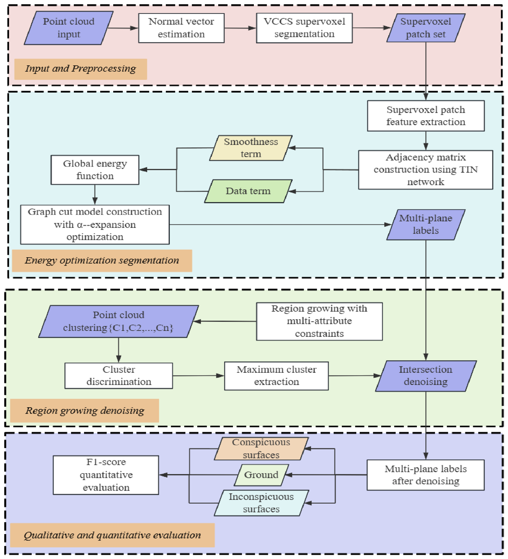
This paper proposes an object-based energy-optimization segmentation method to achieve precise extraction. First, the Voxel Cloud Connectivity Segmentation (VCCS) algorithm is applied to perform supervoxel segmentation on massive point clouds, transforming raw data into semantically consistent point cloud patches. Subsequently, a global energy optimization framework based on graph cut is utilized to achieve a globally optimal segmentation of conspicuous surfaces, inconspicuous surfaces, and the ground via energy minimization. Local refined denoising is then performed via a region-growing algorithm. Finally, the results are evaluated through a combination of qualitative and quantitative assessments. The algorithm flowchart is shown in Figure 1.

2.2. Initial Segmentation Method Based on Supervoxel Clustering

The supervoxel segmentation method [50] converts 3D point clouds into contiguous, semantically coherent regional units. This process transforms massive raw point cloud data into patch structures, reducing the number of processing units and facilitating subsequent energy-optimized segmentation of different planar structures. The specific steps are as follows:

1. Normal Vector Calculation: For any point $p_i$ in the input point cloud $\rho =\left\{p_1,p_2,\dots ,p_N\right\}$, find the $k_{normal}$ nearest neighbors to form the neighborhood ${{\mathcal{N}}_i}^{normal}$, Calculate the centroid $\overline{p_i}$ and construct the covariance matrix $C_i$. Perform eigenvalue decomposition on $C_i$ to obtain three eigenvalues ${\gamma }_0\le {\gamma }_1\le {\gamma }_2$. The eigenvector ${\mathit{\nu }}_{\mathbf{0}}$ corresponding to the smallest eigenvalue ${\gamma }_0$ is the normal vector $n_i$ of $p_i$ where $n_i={\displaystyle \frac{{\mathit{\nu }}_{\mathbf{0}}}{\Vert {\mathit{\nu }}_{\mathbf{0}}\Vert }}$.

$$\{\begin{array}{c}\overline{p_i}={\displaystyle \frac{1}{k_{normal}}}{\sum }_{p\in {{\mathcal{N}}_i}^{normal}}p\\ C_i={\displaystyle \frac{1}{k_{normal}}}{\sum }_{p\in {{\mathcal{N}}_i}^{normal}}(p-\overline{p_i}){(p-\overline{p_i})}^T\end{array}.$$

(1)

2. Supervoxel Grid Construction: For each point $p_i$ with a normal unit $n_i=\left(n_{ix},n_{iy},n_{iz}\right)$ identify the $k_{supervoxel}$ nearest neighbors as its neighborhood ${\mathcal{N}}_i=\left\{p\in \rho |rank\left(\Vert p_i-p\Vert \right)\le k_{supervoxel}\right\}$. Divide the point cloud into uniform 3D voxels using a resolution $R_s$. The grid index for each point is calculated as ${grid}_x\left(p_i\right)$, ${grid}_y\left(p_i\right)$, and ${grid}_z\left(p_i\right)$, where $x_{min}$ is the minimum x-coordinate value of the point cloud, $y_{min}$ is the minimum y-coordinate value of the point cloud, and $z_{min}$ is the minimum z-coordinate value of the point cloud.

$$\{\begin{array}{c}{grid}_x\left(p_i\right)=\lfloor {\displaystyle \frac{x_i-x_{min}}{R_s}}\rfloor \\ {grid}_y\left(p_i\right)=\lfloor {\displaystyle \frac{y_i-y_{min}}{R_s}}\rfloor \\ {grid}_z\left(p_i\right)=\lfloor {\displaystyle \frac{z_i-z_{min}}{R_s}}\rfloor \end{array}.$$

(2)

3. Initial seed point acquisition: Calculate the geometric center of each grid to provide a reference position for subsequent seed point selection. For a grid indexed as $\left(g_x,g_y,g_z\right)$, its center coordinates are $\left(x_c,y_c,z_c\right)$, where $x_c$, $y_c$, and $z_c$. Within each grid, select the real point cloud point closest to the geometric center coordinates $(x_c,y_c,z_c)$ as the initial seed point $r_j$ for the corresponding supervoxel of that grid. Finally, $K$ initial seed points are obtained to form the seed set $\mathcal{R}=\left\{r_1,r_2,\dots ,r_K\right\}$.

4. Supervoxel segmentation: Given two points, $p\left(x_p,y_p,z_p\right)$ and $q(x_q,y_q,z_q)$, the normal vector of point $p$ is $n_p$, and the normal vector of point $q$ is $n_q$. By comprehensively considering the normal dissimilarity and the normalized spatial distance, the final dissimilarity $D\left(p,q\right)$ between the two points is obtained. A smaller dissimilarity value indicates higher similarity between the two points, meaning they are more likely to belong to the same supervoxel:

$$D\left(p,q\right)=1-\left|n_p·n_q\right|+0.4\times {\displaystyle \frac{\Vert p-q\Vert }{R_s}},$$

(3)

$$\Vert p-q\Vert =\sqrt{{(x_p-x_q)}^2+{(y_p-y_q)}^2+{(z_p-z_q)}^2}.$$

(4)

After assigning each point in the point cloud to the nearest seed to obtain the initial segmentation $l_i$, candidate seeds are searched within the point’s KNN neighborhood, collecting all seeds that appear in the neighborhood as ${\mathcal{H}}_i$. The point label is updated to the seed with the minimum neighborhood distance: ${l_i}^{new}$. Based on the new label seeds, the cluster center of each supervoxel is recalculated, its spatial centroid and normal vector are updated, and old visualized points are replaced. Finally, the iteration terminates when the proportion of points with changed labels to the total number of points falls below 0.1%, or when the maximum number of iterations is reached. Consequently, the dense point cloud data is segmented into supervoxel blocks $V=\left\{v_1,v_2,\dots ,v_M\right\}$ with different label values.

$$\{\begin{array}{c}{l}_i={argmin}_{j=1\dots K}D\left(p_i,r_j\right)\\ {\mathcal{H}}_i=\left\{r_j|\exists q{\in \mathcal{N}}_i,l_q=j\right\}\\ {l_i}^{new}={argmin}_{r_j\in {\mathcal{H}}_i}D\left(p_i,r_j\right)\end{array}.$$

(5)

2.3. Accurate Segmentation Method Based on Energy Optimization Model

Following preliminary supervoxel segmentation, the massive raw sonar point cloud is converted into spatially compact and semantically coherent block units, which significantly reduce the computational complexity of subsequent processing. However, due to scattering echo interference in sonar imaging and blurred boundaries between different structural components, the same planar structure is often over-segmented into multiple adjacent supervoxel blocks.

To address this issue, the paper proposes a fine segmentation method based on graph-cut energy optimization [47]. Taking supervoxel blocks as the basic nodes of the graph, the method constructs a global energy function incorporating planar geometric features and minimizes the energy function to achieve a globally optimal aggregation of supervoxels, ultimately obtaining a semantically complete segmentation result for the caisson planes.

2.3.1. The Energy Optimization-Based Segmentation Model

The course of supervoxel segmentation obtains $M$ effective supervoxel blocks, which are mapped to the node set $V=\left\{v_1,v_2,\dots ,v_M\right\}$ of an undirected graph $G=\left(V,\mathrm{ℇ}\right)$. Each node corresponds to a supervoxel block, and each supervoxel block includes a point cloud set $P_i=\left\{p_{i1},p_{i2},\dots ,p_{ini}\right\}$, where $ni$ is the number of points in the supervoxel, and the centroid coordinates are $c_i=\left(x_{ci},y_{ci},z_{ci}\right)$.

The constructed energy function consists of a data term and a smoothness term, and the total energy function is defined as follows:

$$E\left(L\right)=E_{data}\left(L\right)+E_{smooth}\left(L\right),$$

(6)

where $L=\left\{l_1,l_2,\dots ,l_M\right\}$ represents the label assignment of all nodes, and $l_i\in \left\{1,2,\dots ,M\right\}$ indicates the plane category to which node $v_i$ belongs. $E_{data}\left(L\right)$ is the data term, which quantifies the cost of assigning a node to a specific label; $E_{smooth}\left(L\right)$ is the smoothness term, which measures the penalty for label inconsistency between adjacent nodes.

2.3.2. Data Term Construction

The fitted plane parameters are ${\pi }_i=\left(A_i,B_i,C_i,D_i\right)$, which satisfy the plane equation $A_{i}x+B_{i}y+C_{i}z+D_i=0$. The data term $E_{data}\left(L\right)$ is designed to measure the cost of assigning $v_i$ to label $l_i$. This paper constructs the data term by integrating two geometric constraints: plane parallelism and maximum point-to-plane distance.

First, the plane parallelism constraint is established. Supervoxel blocks belonging to the same plane have approximately parallel normal vectors. For planes ${\pi }_i$ and ${\pi }_j$, their unit normal vectors are $n_i$ and $n_j$, and the angle between the normal vectors is ${\theta }_{ij}=arccos\left(\left|n_i\cdot n_j\right|\right)$. Based on the angle, the parallelism cost is defined as follows:

$$C_{parallel}\left(i,j\right)=\{\begin{array}{c}{\displaystyle \frac{{\theta }_{ij}}{{\theta }_{th}}}, {\theta }_{ij}\le {\theta }_{th}\\ 10, {\theta }_{ij}\ge {\theta }_{th}\end{array},$$

(7)

where ${\theta }_{th}$ is the parallelism threshold. When the angle is below the threshold, the parallelism cost is proportional to the angle; when the angle is greater than the threshold, the two planes are considered non-parallel, and a large penalty is imposed.

Then, the maximum distance constraint from the point to the plane is constructed. The formula for the distance from a point to a plane is given by the following:

$$d\left(p,\pi \right)={\displaystyle \frac{\left|Ax+By+Cz+D\right|}{\sqrt{A^2+B^2+C^2}}},$$

(8)

where $p(x,y,z)$ denotes the point coordinates, and $\pi =(A,B,C,D)$ represents the plane parameters.

The maximum distance from supervoxel $v_i$ to plane ${\pi }_j$ is $D_{i\to j}$, and the maximum distance from supervoxel $v_j$ to plane ${\pi }_i$ is $D_{j\to i}$, as given by the following formulas:

$$\{\begin{array}{c}{D}_{i\to j}={\mathrm{m}\mathrm{a}\mathrm{x}}_{p\in P_i}d(p,{\pi }_j)\\ D_{j\to i}={\mathrm{m}\mathrm{a}\mathrm{x}}_{p\in P_j}d(p,{\pi }_i)\end{array}.$$

(9)

Combining the maximum distances in both directions yields the inter-plane distance: $D_{ij}=\mathrm{m}\mathrm{a}\mathrm{x}(D_{i\to j},D_{j\to i})$.

By combining the plane parallelism and the maximum distance from points to the plane, the comprehensive data cost of assigning node $v_i$ to label $l_j$ is obtained:

$$C_{data}\left(i,j\right)=\{\begin{array}{c}{C}_{parallel}\left(i,j\right)\cdot D_{ij}, C_{parallel}\left(i,j\right)<5\\ C_{parallel}\left(i,j\right)\cdot 100, C_{parallel}\left(i,j\right)\ge 5\end{array}.$$

(10)

Finally, the data cost matrix is normalized to the interval [0, 100], and multiplied by the distance weight coefficient ${\alpha }_d$ to obtain the final data term, which balances the relative magnitude between the data term and the smoothness term, ensuring numerical stability during energy minimization.

$$E_{data}\left(L\right)={\alpha }_d{\displaystyle \sum _{i=1}^M}{C}_{data}\left(i,l_i\right).$$

(11)

2.3.3. Adjacency Matrix and Smoothness Term Construction

The edge set $\mathrm{ℇ}$ of the graph is determined by the spatial adjacency relationships between nodes. An adjacency matrix is constructed based on a TIN (Triangulated Irregular Network) network; the adjacency matrix is constructed to generate a spatially continuous adjacency relationship, which conforms to the spatial continuity characteristics of the caisson structure. The smoothness term ensures that spatially adjacent and structurally similar supervoxels are assigned to the same label. This paper adopts the classic Potts model to construct the smoothness term:

$$E_{smooth}\left(L\right)={\sum }_{\left(i,j\right)\in \mathrm{ℇ}}V(l_i,l_j),$$

(12)

$$V\left(l_i,l_j\right)=\{\begin{array}{c}0,l_i=l_j\\ \gamma ,l_i\ne l_j\end{array},$$

(13)

where $V(l_i,l_j)$ is the penalty function for inconsistent labels of adjacent nodes, and $\gamma$ is the penalty weight for label inconsistency between adjacent nodes, which controls the strength of spatial smoothness constraints and balances the relative importance between data fidelity and spatial continuity. A larger weight indicates a stronger tendency for adjacent nodes to be assigned the same label.

2.3.4. The Final Optimization Process

The $\alpha$-expansion algorithm [51] is employed to solve the multi-label energy minimization problem, with the following steps:

1. Initialize the label assignment by setting the initial label of each node to its own index.

2. For each possible label $\alpha$, construct the corresponding binary graph and compute the minimum cut for changing the node label to $\alpha$ or keeping the original label.

3. If the energy corresponding to the minimum cut is less than the current total energy, update the label assignment.

4. Repeat steps 2–3 until the total energy no longer decreases after traversing all labels or the maximum number of iterations is reached; finally, output the final label assignment result $L$ [52].

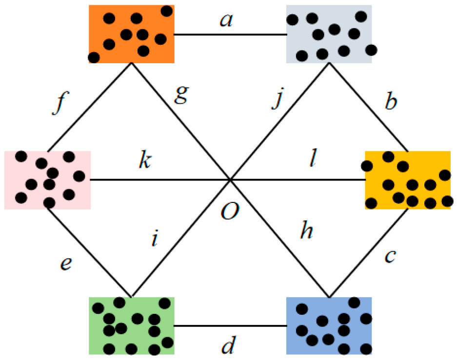
The colored rectangular blocks with point clouds in Figure 2 are semantic units generated via VCCS supervoxel clustering. This step first aggregates massive discrete 3D sonar point clouds into several spatially compact and geometrically consistent supervoxel patches, which significantly reduces the computational complexity of subsequent processing. The connecting lines between the blocks form the topological structure of an undirected graph. Building on this structure, the algorithm constructs a global energy function that integrates a data term and a smoothness term and finally solves for the global minimum of the energy using the α-expansion graph-cut algorithm to assign a globally optimal plane label to each supervoxel. This achieves joint and accurate segmentation of both conspicuous and inconspicuous surfaces, while balancing computational efficiency and the preservation of fine structural details.

2.4. Region-Growing Post-Processing

Suspended particles in water, multipath effect noise, and penetration noise degrade the segmentation performance of 3D sonar point clouds with different labels. To address this issue, this paper proposes a region-growing method [52] with multi-attribute constraints. The method first divides the point cloud into different clusters, and then removes noise clusters by cluster discrimination, extracting the largest point cloud cluster, and intersecting it with the point clouds segmented through energy optimization.

The region-growing algorithm is the process of segmenting the point cloud dataset:

$\rho =\{p_1\left(x_1,y_1,z_1,I_1\right),p_2\left(x_2,y_2,z_2,I_2\right),\dots ,p_m\left(x_m,y_m,z_m,I_m\right)\}$ (where $I_i$ is the intensity value of point $p_i$) into a set of point cloud clusters with different attributes, $Clusters\{C_1,C_2,\dots ,C_n\}$.

The attribute difference $L_{ij}$ between any point $p_i(x_i,y_i,z_i,I_i)$ and $p_j(x_j,y_j,z_j,I_j)$ in A is calculated as follows:

$$L_{ij}=w_x\mid x_i-x_j\mid +w_y\mid y_i-y_j\mid +w_z\mid z_i-z_j\mid +w_I\mid I_i-I_j\mid ,$$

(14)

where $\{w_x$, $w_y$, $w_z$, $w_I\}$ are the weights of each attribute component, with a value range of 0–1.

Based on attribute A, three thresholds are set: $T_d,T_{\theta 1}$, and $T_{\theta 2}$. Specifically, $T_d$ is the distance threshold, $T_{\theta 1}$ is the attribute difference threshold (small), and $T_{\theta 2}$ is the attribute difference threshold (large). The attribute $I$ selected in this paper is the normal vector.

From the unsegmented points in A, point $p$ (the point with the closest plane distance to its own neighborhood of radius r) is included in an empty seed point set $seeds\left\{\right\}$ and a point cloud cluster $C_1\left\{\right\}$, and p is marked as segmented.

Starting from point $p$, all points $P_{nei}\{p_1,p_2,\dots \}$ are found within its neighborhood radius r. For each point $p_i$ in $P_{nei}$, the attribute difference $L_i$ between point $p_i$ and point $p$ satisfies $L_i$ < $T_{\theta 2}$; then, $p_i$ is included in $C_1\left\{\right\}$; if the plane distance $d_i$ from $p_i$ to its own neighborhood of radius r satisfies $d_i$ < $T_d$ and simultaneously $L_i$ < $T_{\theta 1}$, then $p_i$ is also included in $seeds\left\{\right\}$. $p$ is removed from $seeds\left\{\right\}$.

The remaining points in $seeds\left\{\right\}$ are iterated and step 3 is repeated until $seeds\left\{\right\}$ is empty. At this point, the storage of point cloud cluster $C_1$ is complete.

Steps 2–4 are repeated until all points in $\rho$ are segmented. The storage of $Clusters\{C_1,C_2,\dots ,C_n\}$ is complete.

The distance threshold controls the maximum allowed distance from a point to the fitted plane, eliminating outliers while preserving smooth structures. The normal angle thresholds ensure consistency in the surface normal orientations, enabling the differentiation of distinct planes, edges, and noise points. After completing the region-growing denoising method with multi-attribute constraints, the maximum cluster $C_{max}$ is extracted as the main point cloud data. It is then intersected with the point clouds of each label and segmented by energy optimization to accomplish the removal of noise points, resulting in the final denoised outcome of the energy optimization segmentation.

3. Results

3.1. Experimental Data

The hardware of the BV5000 3D sonar system primarily consists of a scanning sonar head, a pan-tilt unit, and a sonar control unit, manufactured by BlueView Technologies, Inc. (now Teledyne BlueView, Inc.), Seattle, Washington, United States. By emitting acoustic waves at a fixed frequency, the system measures the time interval t between the transmission of a pulse signal and the reception of its echo, while simultaneously capturing echo intensity information. The distance L is subsequently calculated based on the travel time t and the velocity of the acoustic waves. In this experiment, seabed data was collected using the BV5000 sonar scanner, resulting in three batches of point cloud data. To provide a detailed account of the experimental process, this paper utilizes the first batch as the primary subject of study. The remaining two batches are employed to verify the generalization capability of the proposed algorithm across different scenarios. All three datasets are used for quantitative evaluation, each with distinct point scales and geometric dimensions. Specifically, Caisson 1 contains 2,359,808 points, with a length of 13.6598 m, a width of 12.6262 m and a height of 10.5340 m. Caisson 2 consists of 2,417,866 points, measuring 13.1451 m in length, 12.8066 m in width and 9.9551 m in height. Caisson 3 has the largest point count of 2,624,672 among the three groups, while its overall size is the smallest, with a length, width and height of 12.3841 m, 11.8867 m and 8.7316 m respectively. 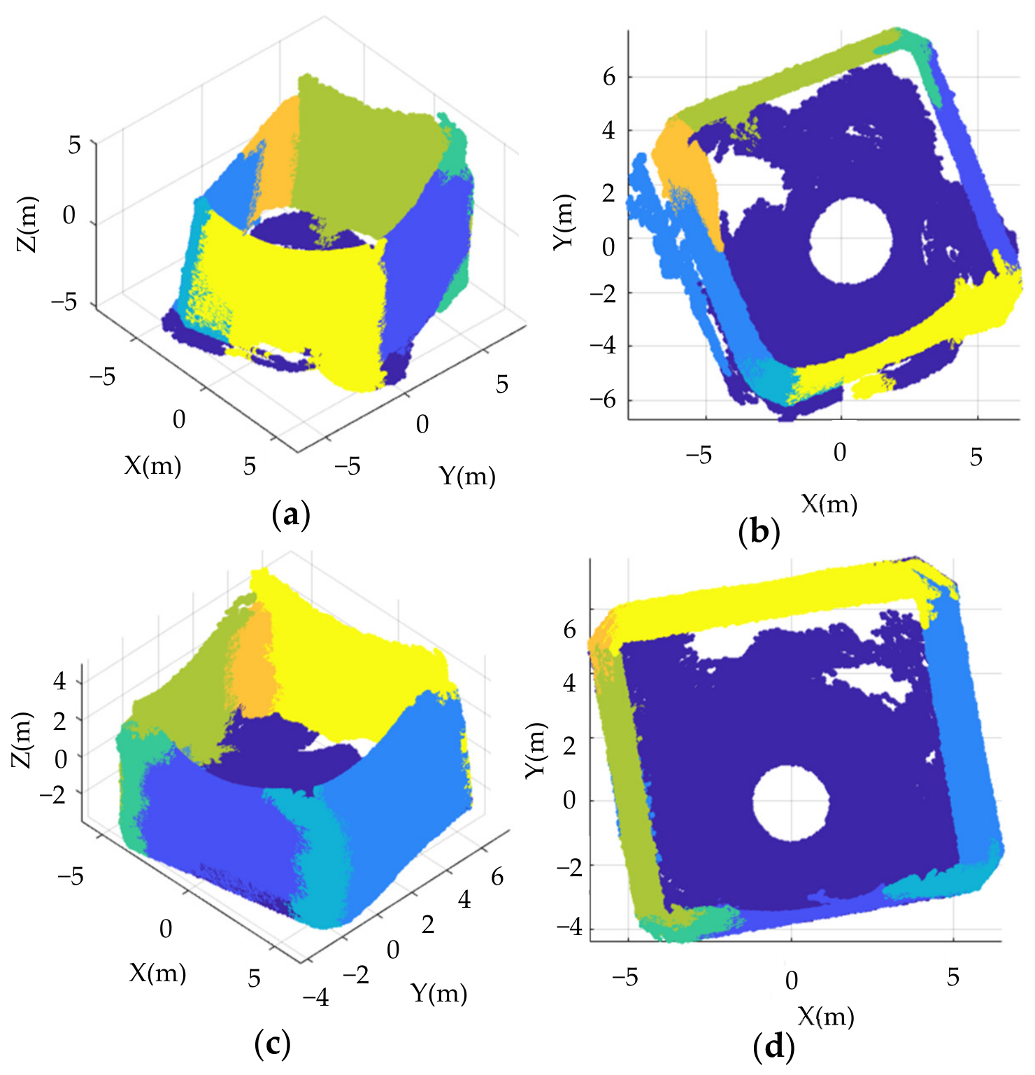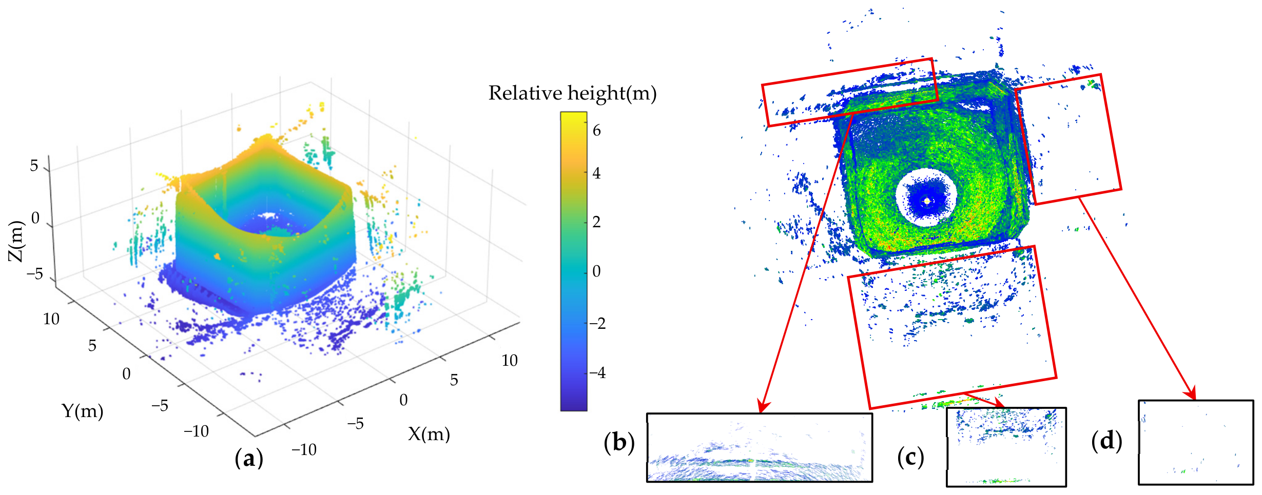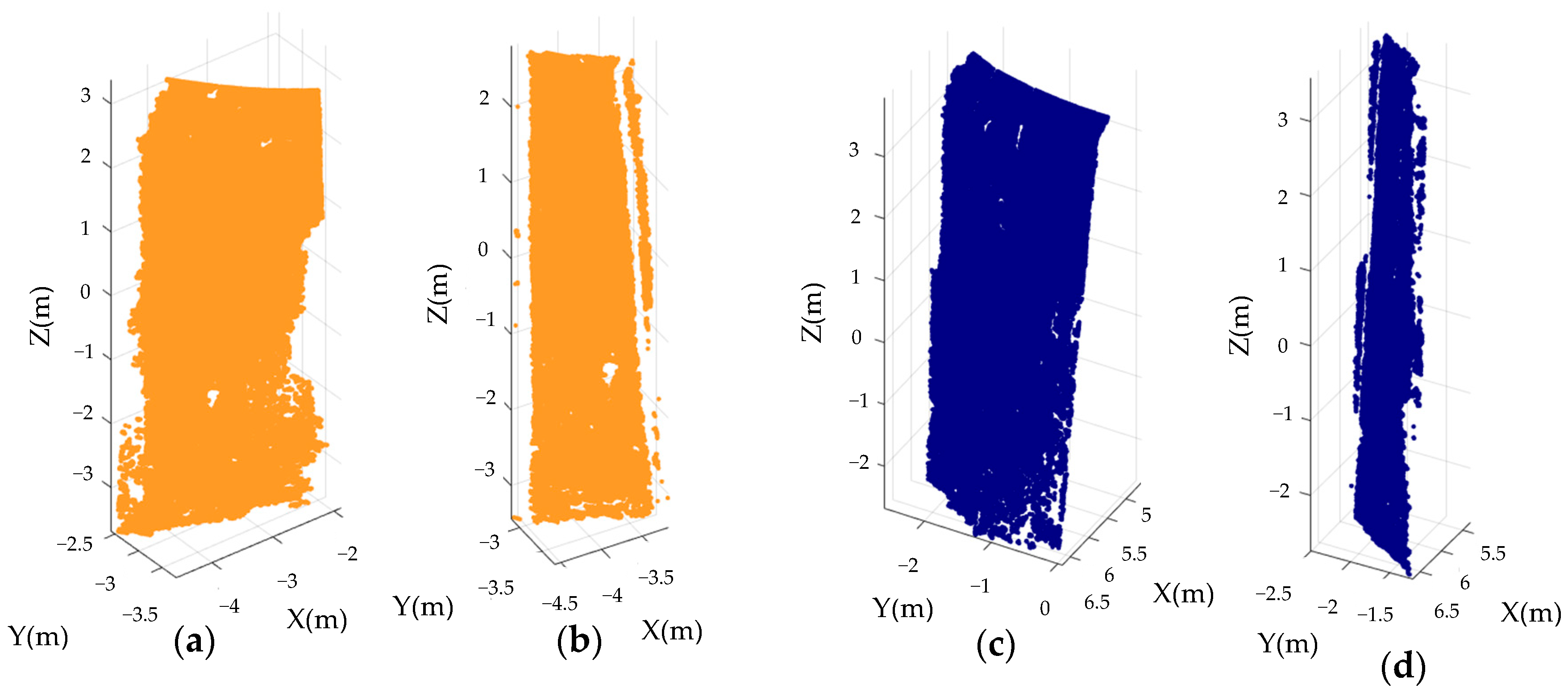Figure 3 below displays the 3D visualization results of the first batch of point cloud data.

Since acoustic waves are received after multiple reflections, the observed distance tends to be overestimated, manifesting as offset or layered sheet-like anomalies within the point cloud. As shown in Figure 3c, sonar possesses a certain degree of penetration capability. As illustrated in Figure 3d, these noise clusters typically exhibit low density.

3.2. Accuracy Assessment Metrics

To ensure the reproducibility and validity of the reported quantitative results, this section explicitly details the construction of the reference ground truth, the matching strategy between predicted and reference regions, and the F1-score calculation procedure. Since no public benchmark dataset with pixel-level annotations exists for underwater 3D sonar point clouds of caisson structures, a high-precision reference ground truth was manually constructed for each dataset. An experienced operator utilized CloudCompare software(v2.14 alpha) to perform semantic annotation on the raw point clouds, carefully delineating the boundaries of conspicuous surfaces, inconspicuous surfaces, and the ground plane based on geometric continuity and structural priors. We manually distinguish between conspicuous and inconspicuous surfaces through visual inspection directly in CloudCompare and determine the segmentation accuracy based on point-wise labels. To minimize subjective bias and annotation artifacts, all manual labels were subsequently verified and refined by a second independent expert.

The reference ground truth consists of manually annotated point-wise semantic labels. The resulting annotated point clouds serve exclusively as the immutable reference standard (ground truth) for evaluating segmentation accuracy and are not treated as a competing algorithmic method in the primary performance comparison.

A point pair was considered a valid match only when each point was the nearest neighbor of the other within 0.01 m, ensuring bidirectional consistency and eliminating ambiguous one-way matches.

Based on the set of matched reciprocal correspondences, True Positives ($tp$) were the number of points in the predicted cloud that had a valid reciprocal correspondence in the reference cloud. False positives ($fp$) were the number of points in the predicted cloud that did not have a valid reciprocal correspondence, and False Negatives ($fn$) were the number of points in the reference cloud that did not have a valid reciprocal correspondence:

$Precision$, $recall$, and $F1\text{-}score$ were then computed as follows [53]:

$$Precision=100\ast {\displaystyle \frac{tp}{tp+fp}}\%,$$

(15)

$$Recall=100\ast {\displaystyle \frac{tp}{tp+fn}}\%,$$

(16)

$$F1\text{-}score={\displaystyle \frac{2\ast Precision\ast Recall}{Precision+Recall}},$$

(17)

3.3. Experimental Results and Quantitative Evaluation

The experiments were conducted on a laptop computing platform with the following hardware specifications: a 13th Gen Intel^® Core™ i9-13980HX processor with a base frequency of 2.20 GHz, 16.0 GB of onboard RAM, a discrete NVIDIA GeForce RTX 4060 Laptop GPU with 8 GB of dedicated video memory, and an integrated Intel^® UHD Graphics with 128 MB of graphics memory.

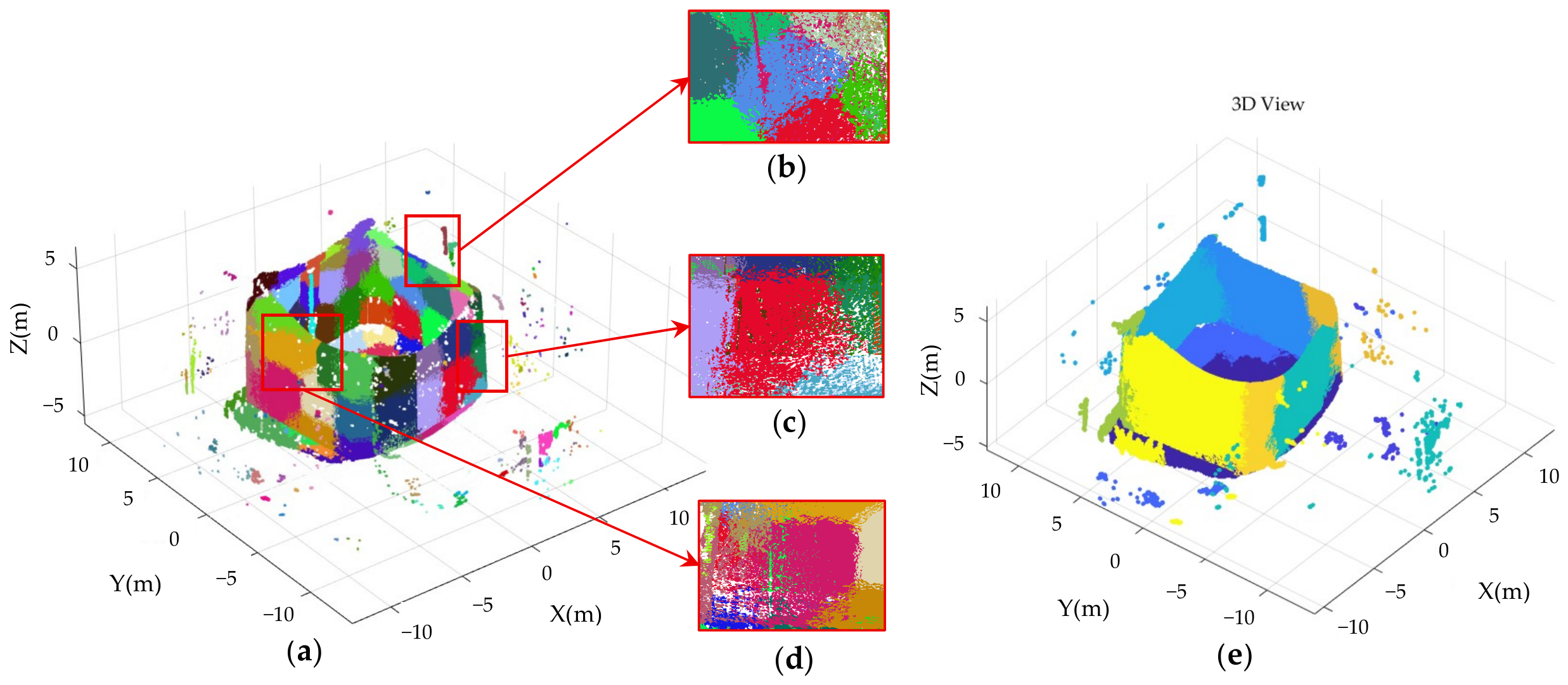
First, supervoxel point cloud segmentation was conducted to reduce the computational load for subsequent processing and transform the point clouds into semantically consistent objects. In the supervoxel segmentation process, considering the high density of the sonar point clouds, the number of nearest neighbors for normal vector estimation $k_{normal}$ was set to 15 to balance noise reduction and precision. Given the large scale of the engineering structures and their planar characteristics, the supervoxel resolution $R_s$ was set to 3.5 to control the size of the supervoxels and prevent the loss of structural details. Furthermore, to accommodate the dense yet potentially non-uniform distribution of points on these planar surfaces. The number of nearest neighbors for supervoxel clustering $k_{supervoxel}$ was set to 20 to ensure connectivity and adapt to the non-uniform density of the sonar point clouds. Based on this coarse segmentation, the massive, high-density point cloud data was divided into spatially compact, internally connected blocks with distinct features. The boundaries of these blocks closely align with the structural edges, and the blocks are more stable than the raw point cloud data.

The supervoxel results are shown in Figure 4, where different colors represent point cloud blocks with different features.

Next, the conspicuous surfaces, inconspicuous surfaces, and the ground were segmented using the energy optimization model. To control the penalty intensity for inconsistent labels between adjacent supervoxels, the smoothness term weight $\gamma$ was set to 150, favoring the merging of adjacent supervoxels to maintain the integrity of the large-area planar structures. The plane parallelism threshold ${\theta }_{th}$ was set to 35°; values exceeding this threshold incurred high penalties, effectively preserving structural details and maintaining the sections between two nearly perpendicular planes. Crucially, due to the high point density and the presence of multiple parallel planar structures in the data, the distance weight coefficient ${\alpha }_d$ was set to 10, providing a strong constraint for plane distance to prevent parallel conspicuous surfaces from being misidentified as the same plane. Finally, fine segmentation was completed using the $\alpha$-expansion algorithm, effectively dividing the point cloud into multiple planar blocks. The parameters were determined through small-scale preliminary tests and subsequently applied to the full datasets. As shown in Figure 4e, the point cloud was divided into eight valid clusters. Due to uneven resolution and confusion at the intersection of the two planes, one inconspicuous surface was not fully recognized; however, because its point count was very low, this did not impact the final quantitative evaluation results.

Due to the influence of multipath reflections, suspended particles in the water, and electronic interference, the data is prone to containing randomly distributed, unstructured noise points. To address this, a region-growing denoising algorithm with multi-attribute constraints was applied to the first batch of data. Since the point cloud density is medium with small point intervals, the search radius for normal estimation K was set to 30 to prevent over-smoothing and the loss of detail inherent in dense planar data. Simultaneously, taking advantage of the tight spatial distribution of points on the planes, the distance threshold $T_d$ was set to 0.01 to filter out outliers caused by acoustic scattering, multipath reflections, or penetration while avoiding the excessive removal of real structural points.

The small normal angle threshold $T_{\theta 1}$ was set to 10°, and the large normal angle threshold $T_{\theta 2}$ was set to 20° to effectively suppress aggregated noise with large normal variations while tolerating reasonable fluctuations caused by sparse sampling, ensuring that the distinct planar features are preserved during denoising. This algorithm divided the point cloud into several clusters; clusters representing distant noise, suspended particles, or multipath interference were removed, and the largest cluster (the structure and terrain) was retained to complete the denoising of the energy-optimized segmentation.

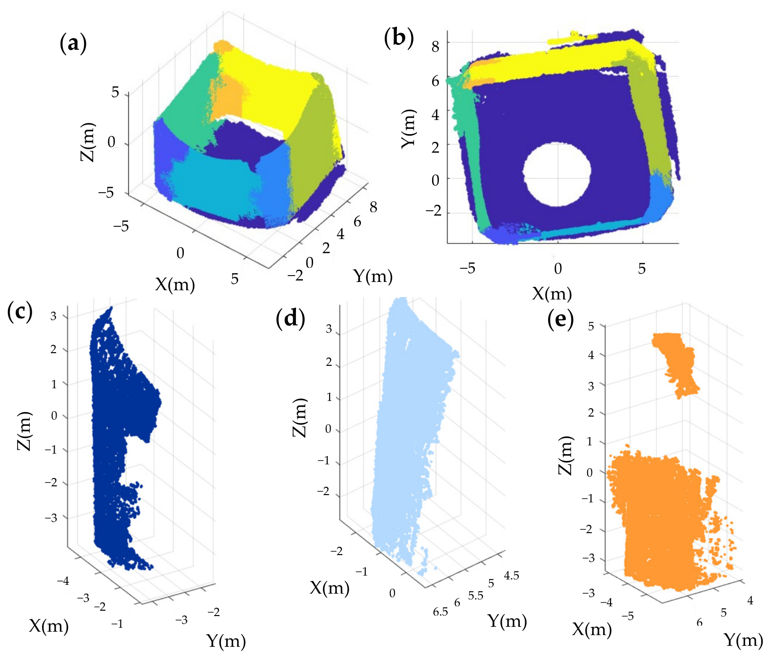
The denoised results are shown in Figure 4, and the energy-optimized segmentation after noise removal is shown in Figure 5.

Following the evaluation method in the literature [53], to verify the generalization and robustness of the algorithm proposed in this paper, data from two additional caissons were introduced. The specific results are shown in Figure 6.

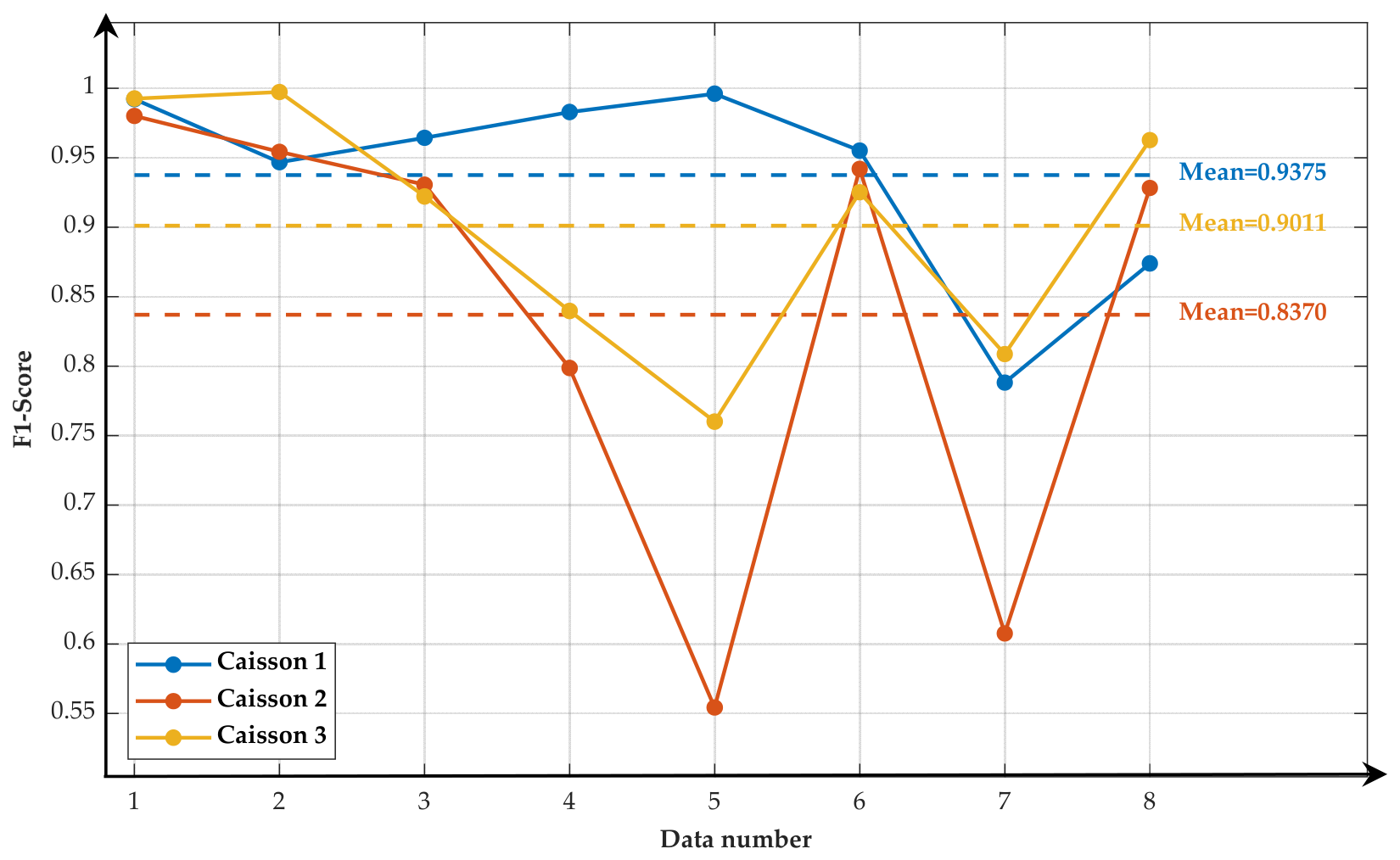
As shown in Figure 7, for the main experimental dataset of Caisson 1, the algorithm in this paper achieved precise segmentation of the eight core planar structures of the caisson. Only one inconspicuous surface, which accounted for an extremely low proportion of the point cloud and was in the boundary region between planes, was not fully recognized; this had no impact on the integrity of the main structure. Quantitative results show that the average F1-score of Caisson 1 reached 0.9375, Caisson 2 reached 0.8370, and Caisson 3 reached 0.9011. The algorithm achieved high F1-scores for the segmentation of typical planar structures such as conspicuous surfaces, inconspicuous surfaces, and the ground. The segmentation accuracy of each target plane was stable, and the overall average F1-score was 0.892, which is at a high level.

This effectively solves the problem of insufficient segmentation accuracy caused by blurred structural boundaries, interlaced planar structures, and acoustic scattering interference in 3D sonar point clouds, accurately restoring the spatial geometric features of the caisson structure. Moreover, the algorithm demonstrates outstanding generalization and robustness against interference. Generalization verification was conducted using two sets of caisson point cloud datasets under different working conditions (Caisson 2 and Caisson 3). The quantitative results indicate that the proposed algorithm maintains stable segmentation performance in test scenarios with varying point cloud densities, noise interference intensities, and structural scales.

The overall average F1-scores of the three sets of test data were all maintained at a high level, proving that the algorithm has strong anti-interference capabilities against three typical types of noise in underwater sonar point clouds (scattering effect noise, multipath reflection noise, and penetration noise), possesses good scenario adaptability for complex caisson structures of different shapes, and satisfies the robustness requirements for practical engineering applications.

Quantitative evaluation is essential for distinguishing performance differences among high-quality segmentation results, as visual inspection alone is insufficient when processing large-scale point clouds with subtle numerical variations, as shown in Figure 4, Figure 5 and Figure 6. Furthermore, the sensitivity analysis of the spatial distance weight parameter indicates that it exerts a negligible influence on the final segmentation accuracy; therefore, its corresponding quantitative results are omitted to maintain conciseness.

3.4. Other Data Validation

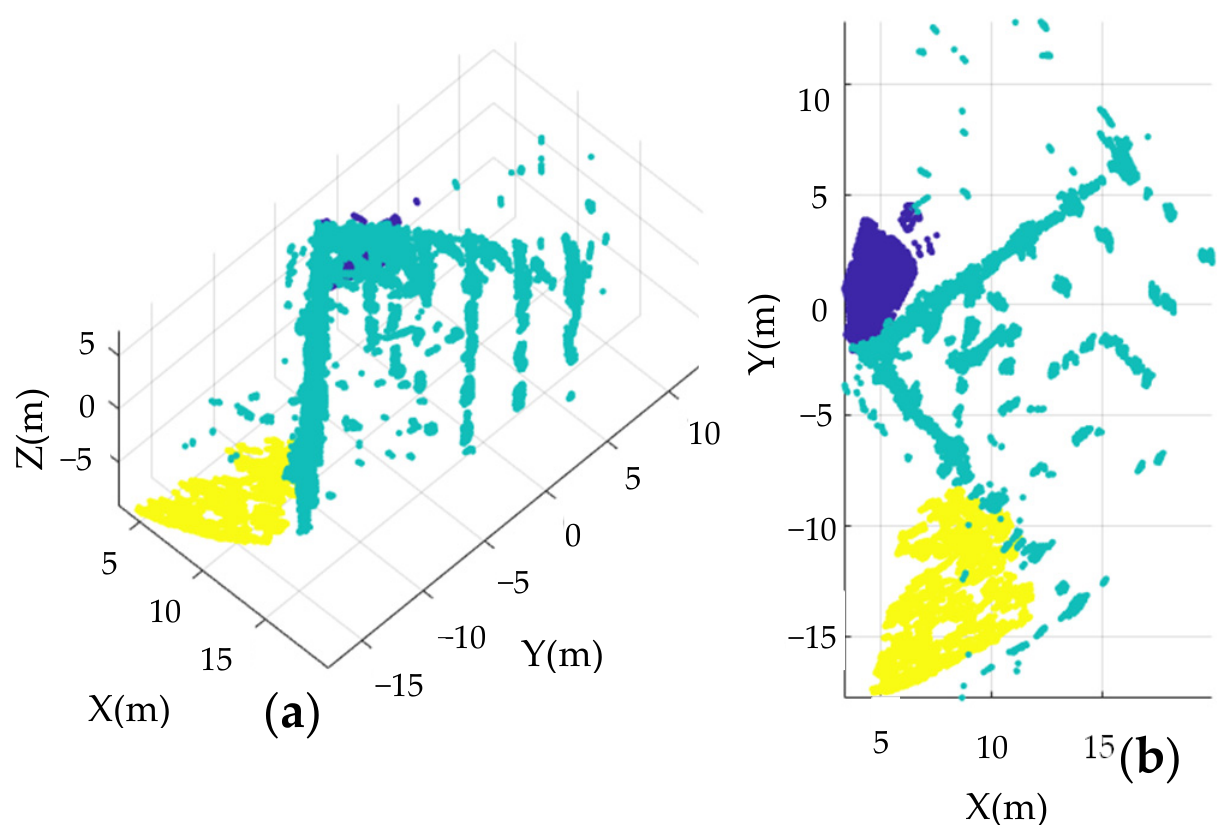
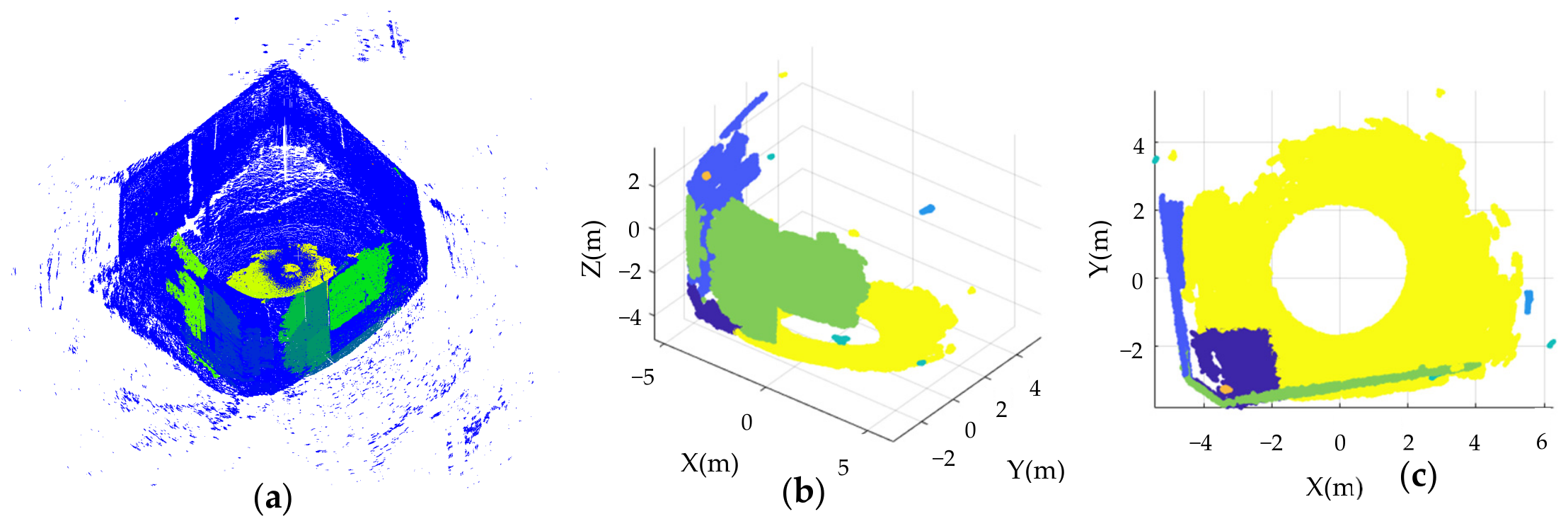
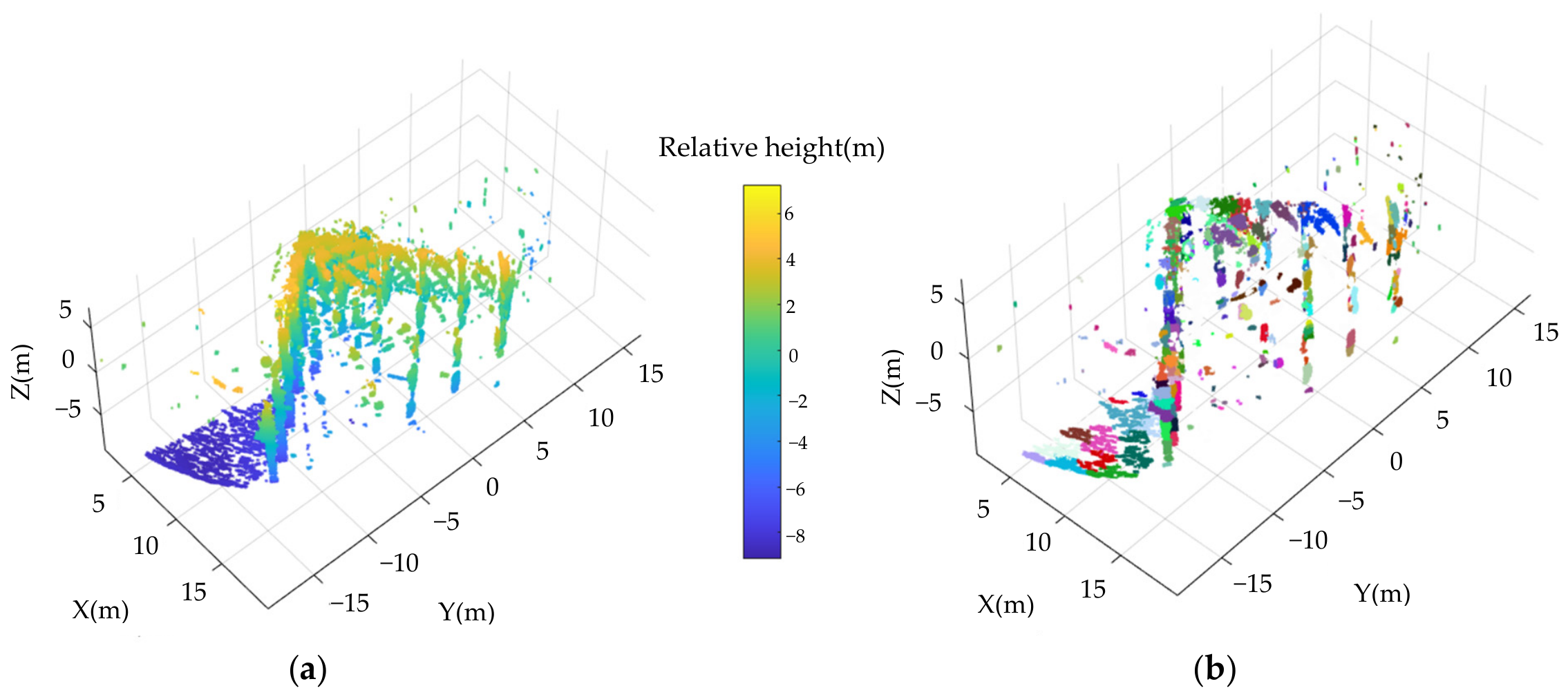
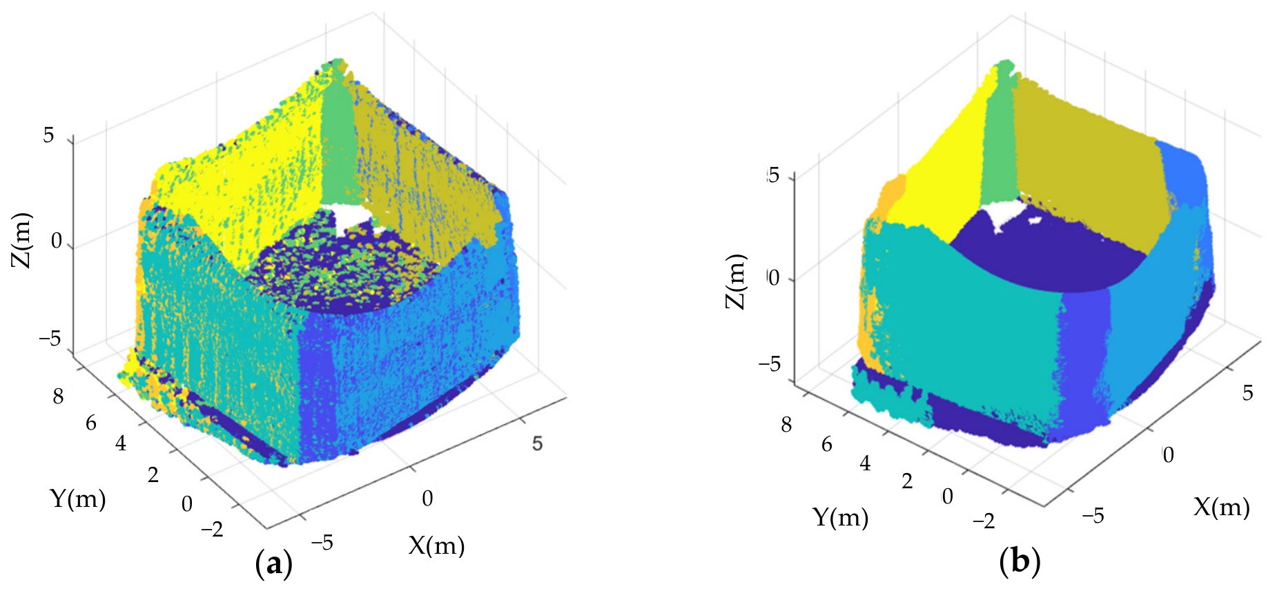
To further verify the generalization and robustness of the proposed algorithm, an additional test set featuring irregular seabed columnar structures was introduced. This dataset comprises large-scale main structures (conspicuous surfaces) coupled with numerous small-scale columnar regions (inconspicuous surfaces) located at structural joints. The point clouds in this batch are characterized by uneven density and blurred boundaries due to intense underwater multipath effects and acoustic scattering, posing a significant challenge for traditional algorithms to preserve local geometric features. The structure is shown in Figure 8a.

The validation process first employed the VCCS supervoxel clustering algorithm to transform the massive discrete point clouds into semantically consistent object patches, significantly reducing computational complexity while preserving geometric micro-details. The structure is shown in Figure 8b. Subsequently, the global energy optimization model was applied for refined segmentation.

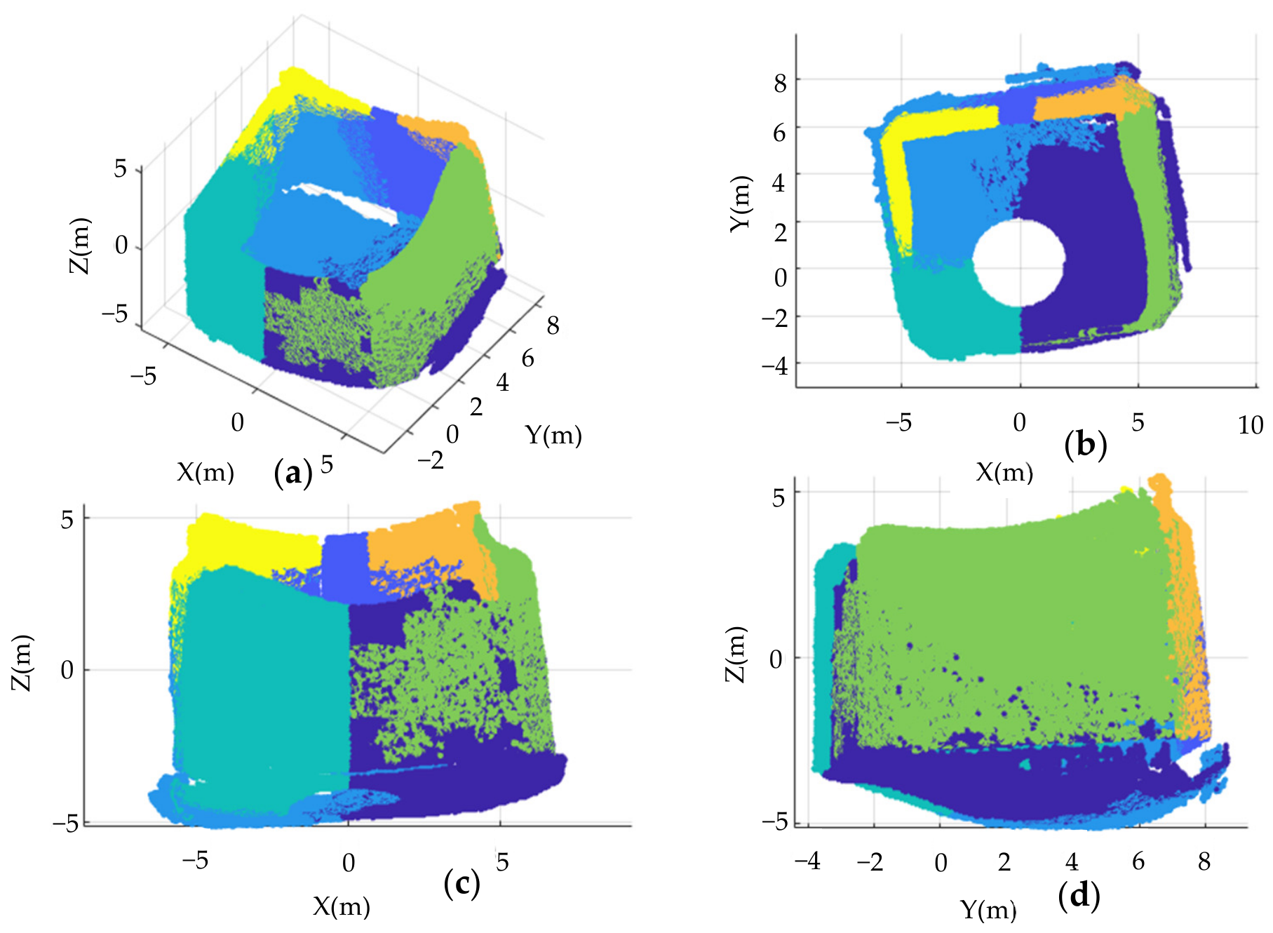
By dynamically balancing the smoothness and data terms, the model ensured the high integrity of large-area planes while accurately extracting the small-scale columnar structures that are typically susceptible to being filtered out as noise or over-merged by traditional methods. The structure is shown in Figure 9.

Quantitative evaluation using the F1-score confirms the high accuracy of the method, with an overall average F1-score of 0.8811. Specifically, the algorithm achieved a robust F1-score of 0.8287 for the challenging columnar inconspicuous surfaces, while the regular planar regions reached accuracies of 0.9661 and 0.8486. These results demonstrate that the proposed method possesses excellent scenario adaptability and maintains stable segmentation performance even when facing complex geometries with sparse and noisy point cloud distributions.

4. Discussion

4.1. Parameter Sensitivity Analysis

To further evaluate the robustness and stability of the proposed algorithm, a parameter sensitivity experiment was conducted. In this experiment, the parameters for initial supervoxel clustering and region-growing denoising remained constant, while only the core hyperparameters within the global energy optimization model were adjusted. Specifically, the adjustments focused on three key variables: smoothness term weight $\gamma$; the plane parallelism threshold ${\theta }_{th}$; and the distance weight coefficient ${\alpha }_d$.

Specifically, the four parameter groups are defined as follows: Parameter Group 1: $\gamma$ = 100, ${\theta }_{th}$ = 35°, and ${\alpha }_d$ = 10; Parameter Group 2: $\gamma$ = 150, ${\theta }_{th}$ = 35°, and ${\alpha }_d$ = 20; Parameter Group 3: $\gamma$ = 150, ${\theta }_{th}$ = 35°, and ${\alpha }_d$ = 30, and Parameter Group 4: $\gamma$ = 200, ${\theta }_{th}$ = 35°, and ${\alpha }_d$ = 10. The segmentation performance of these configurations was thoroughly tested across the three batches of caisson datasets (Caisson 1, Caisson 2, and Caisson 3). In the accompanying visual representation, the same colors are utilized to denote identical parameter configurations across the different caissons, facilitating a direct and intuitive comparison of their extraction effectiveness, as shown in

Table 1. Parameter sensitivity analysis results.

	F1-Score of Caisson 1	F1-Score of Caisson 2	F1-Score of Caisson 3
Parameter Group 1	0.8065	0.8659	0.9011
Parameter Group 2	0.8065	0.8659	0.9011
Parameter Group 3	0.8065	0.8659	0.9011
Parameter Group 4	0.9375	0.8659	0.9011

.

The quantitative evaluation reveals that the final average F1-scores for the four parameter groups are 0.8578, 0.8578, 0.8578, and 0.9015, respectively. These results strongly demonstrate the parameter insensitivity of the proposed method and provide two critical insights: First, despite significant variations in the hyperparameter configurations (such as doubling the smoothness penalty $\gamma$ or tripling the distance weight ${\alpha }_d$), the algorithm’s average F1-score consistently stabilizes at a robust baseline of approximately 0.8578. This illustrates that the overall energy optimization framework possesses strong fault tolerance. It does not rely on meticulous hyperparameter fine-tuning to function effectively; even when parameters deviate from their optimal values, the structural integrity and high-accuracy segmentation of complex transitional boundaries are well-maintained. Second, while the optimal parameter combination (Parameter Group 4) effectively balances the spatial smoothness penalty and the geometric data constraints to yield a peak average F1-score of 0.9015, the performance gap between the different configurations remains remarkably narrow.

In conclusion, the proposed energy optimization segmentation model exhibits remarkable parameter insensitivity. This highly stable characteristic ensures that the algorithm can robustly adapt to varying underwater point cloud densities, noise levels, and structural complexities without demanding stringent and time-consuming manual parameter calibration, thus significantly enhancing its deployment potential in practical underwater engineering applications.

4.2. Method Comparison

To verify the segmentation capability of the algorithm proposed in this paper for different surfaces, a RANSAC algorithm based on Cloth Simulation Filtering (CSF) was introduced, hereafter referred to as CSF-RANSAC. This method first uses CSF to directly separate the ground and structures in the data and then uses RANSAC to fit the planes of the structures, retaining the inliers of all planes as the final RANSAC result. The plane fitting distance threshold $d_{th}$ is set to 0.05 m in this paper. This configuration suppresses the interference of sonar scattering noise while ensuring the fitting integrity of inclined transition wall surfaces. The absolute value threshold of the Z-component of the normal vector $n_{z,max}$ is set to 0.8, which filters out residual horizontal ground points and effectively preserves the geometric details of various inclined surfaces. The minimum number of inliers for valid planes $N_{min}$ is set to 50. While suppressing noise-induced pseudo-planes, this setting also maintains the extraction capability for small-sized non-salient wall surfaces. This algorithm has some flaws regarding point cloud completeness, but the quantity is far less than the total magnitude of the point cloud and can be ignored. 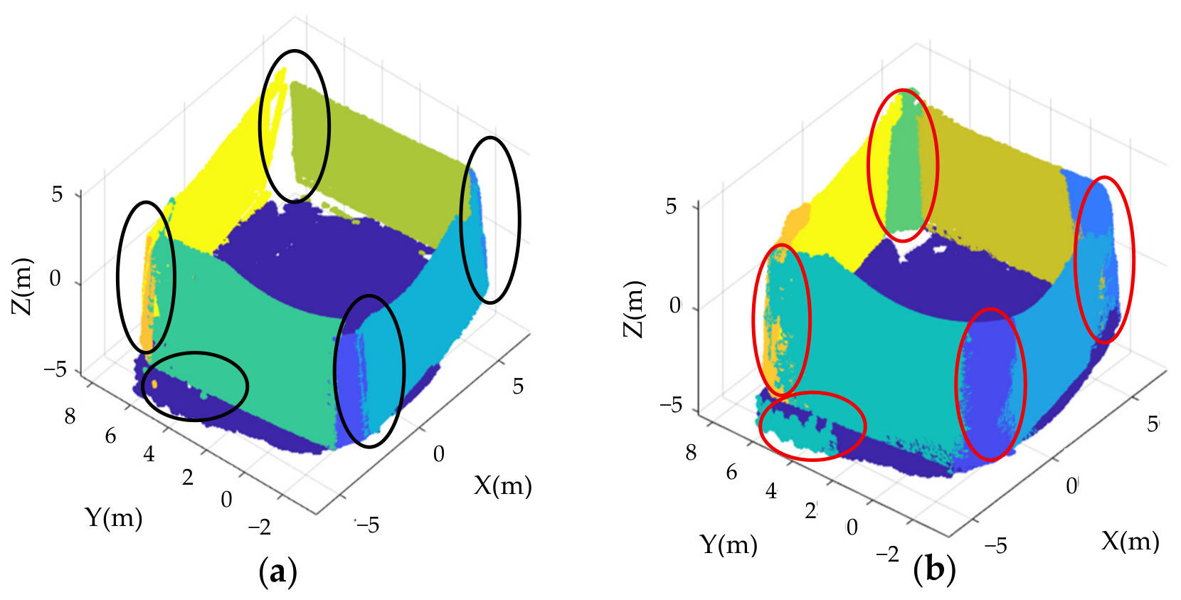At this time, the results are shown in Figure 10 and Figure 11 below. CSF-RANSAC extracts planes very accurately, but inconspicuous surfaces are not just single planes; they are facade structures composed of multiple structures. Furthermore, the inliers retained by CSF-RANSAC suffer from significant point cloud loss, leading to a deficiency in the complete segmentation of conspicuous structural surfaces. From the black-bordered sections in Figure 10a,b, it can be directly seen that CSF-RANSAC is insensitive to small inclined planes, resulting in incomplete plane segmentation.

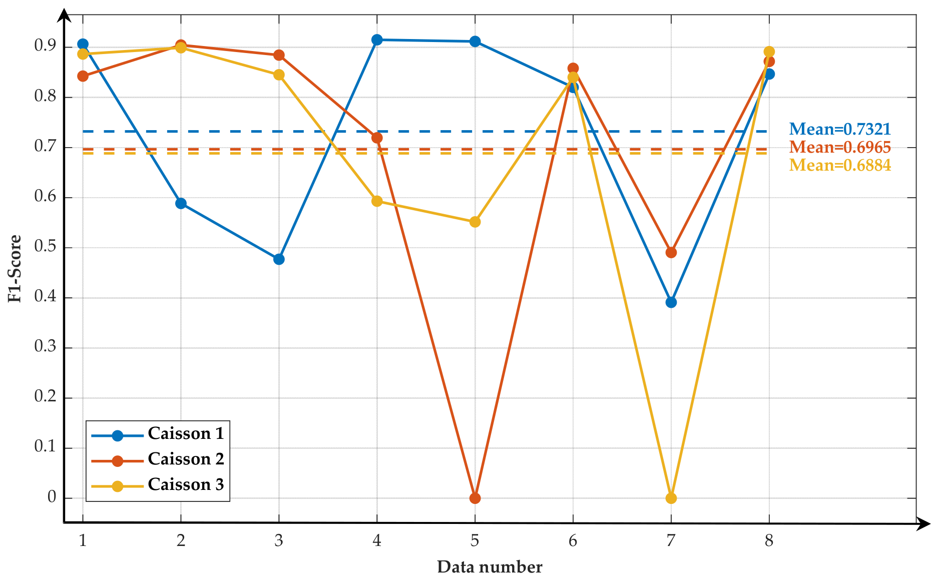
In the quantitative evaluation, the results are shown in Figure 12 below.

As can be seen from the quantitative experiments shown in Figure 12, the CSF-RANSAC algorithm can only filter inliers for a single plane through local sampling and model matching, failing to balance the geometric correlation and global semantic consistency between different planes. When facing complex structures with interlaced multi-planes and blurred boundaries among conspicuous surfaces, inconspicuous surfaces, and the ground, this algorithm frequently mis-merges adjacent planes and under-segments inconspicuous surfaces in plane boundary regions. For inclined transition inconspicuous surfaces between two perpendicular planes, there are large areas that cannot be recognized, and the plane fitting targets have missing point clouds, failing to balance the geometric correlation and global semantic consistency between different planes. The F1-score values for the three batches of data are 0.7321, 0.6965, and 0.6884, respectively, directly reflecting the inaccuracy of the CSF-RANSAC method. The overall average F1-score for the three batches of caisson data is 0.7057, which presents a significant gap compared to the average F1-score of 0.892 achieved by the proposed method across the three datasets. Notably, for the main experimental dataset of Caisson 1, the F1-score of the proposed method improved by 28.06% compared to the baseline algorithm. Even in Caisson 2 data, which has the strongest noise interference and the most complex structure, the improvement reached 20.18%, and as noise intensity and structural complexity increased, the segmentation accuracy of the CSF-RANSAC algorithm dropped significantly. Traditional global energy optimization methods are limited by the plane quantity penalty mechanism of the label cost term and the minimum valid point count threshold for planes, resulting in substantial under-segmentation of inconspicuous surfaces with very few points. In contrast, the proposed method, constrained by the supervoxel neighborhood smoothness term, significantly enhances the recognition capability for small-scale inconspicuous surfaces without increasing the risk of over-segmentation, further demonstrating the accuracy of the proposed method in point cloud segmentation.

In addition to the model-driven CSF-RANSAC approach, traditional normal-based segmentation was also evaluated as a representative feature-driven baseline (Figure 13). While this method exploits local surface orientation for clustering without requiring predefined geometric models, it exhibits fundamental limitations when applied to noisy underwater sonar point clouds of caisson structures. As shown in the subsequent visual results, normal vector segmentation is highly sensitive to noise-induced orientation variations, leading to pervasive missed segmentation and mis-segmentation on ostensibly planar surfaces: continuous planes are frequently fractured into multiple inconsistent clusters, while adjacent distinct planes are erroneously merged due to similar normal estimates in low-resolution or grazing-incidence regions. More critically, fine structural details of inconspicuous surfaces—such as narrow edges, small protrusions, bolt holes, and low-reflectivity transition zones—are systematically omitted because their sparse point distributions and ambiguous geometric signatures fail to form coherent normal-based clusters.

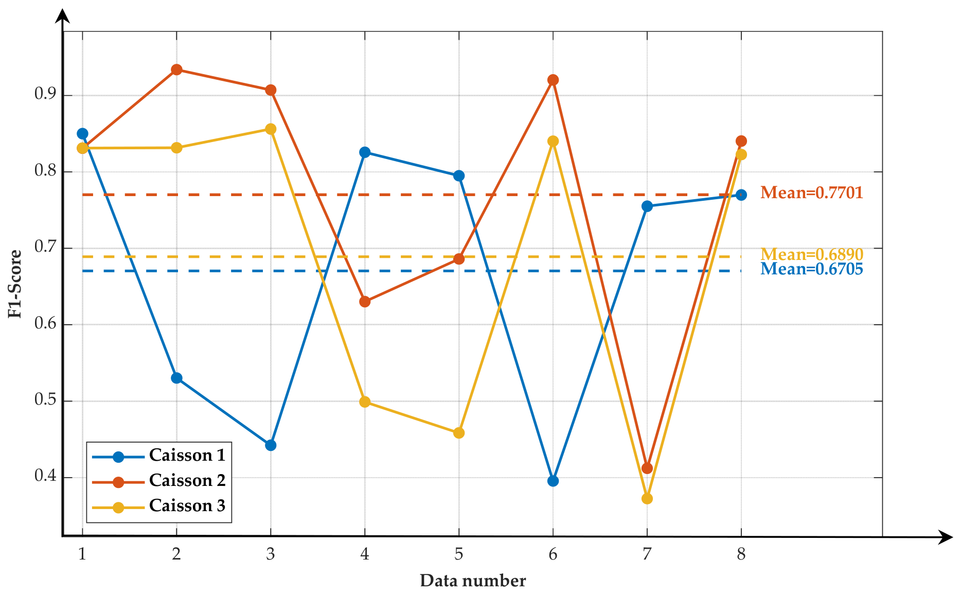
These qualitative deficiencies are corroborated by quantitative evaluation: the average F1-scores for the three batches of caisson data using the normal vector method were only 0.7701, 0.6890, and 0.6705, respectively, with a clear degradation trend across increasingly complex scenes (Figure 14). In stark contrast, the proposed energy optimization method integrates global contextual constraints with local geometric fidelity through a unified minimization framework, enabling robust boundary preservation, noise suppression, and recovery of subtle non-dominant features that purely local feature-based methods inherently miss. The significant performance gap thus confirms that accurate segmentation of both conspicuous and inconspicuous surfaces in real-world underwater environments necessitates a global optimization strategy beyond conventional normal vector clustering.

The main advantage of global energy optimization segmentation lies in its ability to comprehensively consider both neighborhood information and data feature information. Other algorithms, such as region growing, can only consider a single type of neighborhood information; methods like RANSAC can only consider a single type of feature information; and both are unable to accurately and comprehensively depict the overall and local characteristics of underwater structures. The relevant analysis statement has been supplemented.

4.3. Time Efficiency Analysis

To comprehensively evaluate the practical applicability of the proposed method, time efficiency was analyzed alongside segmentation accuracy using the Caisson 1 dataset as a benchmark.

Table 2. Accuracy and time efficiency results.

	Precision	Recall	F1-Score	Time Cost
Energy-based in Caisson 1	0.935339	0.946019	0.937509	645.5566 s
CSF-RANSAC in Caisson 1	0.86703	0.652971	0.732106625	653.582 s
Normal-based in Caisson 1	0.596495	0.696855	0.670464875	938.998 s

presents the quantitative comparison of precision, recall, F1-score, and time cost among the proposed energy-based method, CSF-RANSAC, and normal-based segmentation.

As illustrated in Table 2, the proposed energy optimization method demonstrates superior comprehensive performance by achieving an optimal balance between computational efficiency and segmentation accuracy. In terms of time cost, the proposed method (645.56 s) is slightly faster than the CSF-RANSAC baseline (653.58 s) and significantly outperforms the normal-based method (938.99 s), reducing processing time by approximately 31.3% compared to the latter. This efficiency gain is primarily attributed to the VCCS supervoxel clustering strategy employed in the initial stage, which transforms massive discrete point clouds into semantically consistent patch units, thereby drastically reducing the number of nodes in the subsequent graph-cut optimization and avoiding the computationally expensive point-wise traversal characteristic of traditional feature-driven clustering methods.

More importantly, unlike conventional approaches where higher efficiency often necessitates a compromise in accuracy, the proposed method achieves the highest F1-score (0.9375) while maintaining the lowest time consumption. Although CSF-RANSAC exhibits a comparable processing speed, its F1-score is 20.54% lower than that of the proposed method due to severe under-segmentation of inconspicuous surfaces and point cloud loss. Conversely, while the normal-based method avoids complex model fitting, its reliance on exhaustive local neighborhood searches results in the longest processing time and the lowest segmentation accuracy. Therefore, the quantitative evidence confirms that the proposed object-based energy optimization framework not only ensures high-precision joint extraction of conspicuous and inconspicuous surfaces but also possesses sufficient computational efficiency to meet the timeliness requirements of practical underwater engineering monitoring, demonstrating significant advantages over existing geometric fitting and feature clustering baselines.

4.4. Ablation Experiment

To verify the necessity and effectiveness of each core component in the proposed method, ablation experiments were conducted on the Caisson 1 dataset. The experiments evaluated three variants: (1) replacing VCCS with PCL-based supervoxel segmentation; (2) removing the energy optimization model; and (3) omitting region-growing denoising post-processing. The results demonstrate that all three steps are indispensable for achieving high-precision segmentation of complex underwater structures.

In this experiment, the VCCS algorithm was replaced by the standard supervoxel segmentation method provided in the Point Cloud Library (PCL) to assess the impact of the initial clustering strategy. As shown in Figure 15a, the PCL-based approach failed to generate semantically consistent patches that align with structural boundaries. Due to its insensitivity to the geometric features specific to sonar point clouds, it could not segment out complete structural units. Consequently, the subsequent segmentation pipeline produced fragmented and incomplete results, where both conspicuous and inconspicuous surfaces were severely under-segmented or erroneously merged. This confirms that the VCCS algorithm is superior in preserving structural integrity and providing a reliable object-level foundation for energy optimization in underwater scenarios.

This variant evaluates the contribution of the global energy optimization framework by relying solely on the initial VCCS supervoxel clustering without graph-cut refinement. As illustrated in Figure 16, although VCCS effectively reduces data complexity, the absence of energy optimization leads to excessive over-segmentation. The resulting planes are highly diverse and fragmented, failing to merge adjacent supervoxels belonging to the same physical surface. More critically, this baseline cannot distinguish between significant planar regions and noise-like clusters, nor can it precisely delineate inconspicuous transition surfaces from dominant planes. The inability to enforce spatial smoothness and geometric consistency validates the necessity of the proposed energy optimization model for achieving semantically meaningful and accurate plane extraction.

To quantify the impact of the multi-attribute constrained region-growing denoising step, the full segmentation pipeline was executed without this post-processing stage. Quantitative evaluation reveals that the average F1-score decreased from 0.9375 to 0.9186 when denoising was omitted. Although the energy optimization model possesses inherent robustness, residual scattering noise, multipath artifacts, and suspended particles inevitably persist in the raw sonar data, leading to false positive clusters and boundary inaccuracies. The 1.89% drop in precision demonstrates that the region-growing denoising module is essential for filtering typical sonar-specific noise and refining the final segmentation output to meet high-accuracy engineering requirements.

In summary, the ablation studies conclusively validate the rationality of the proposed three-stage framework. The VCCS supervoxel clustering ensures structurally coherent processing units; the energy optimization model enables precise joint extraction of conspicuous and inconspicuous surfaces; and region-growing denoising guarantees the removal of acoustic interference. Removing any single component significantly degrades either the qualitative completeness or the quantitative accuracy of the segmentation results.

4.5. Denoising Effectiveness

It is imperative to first clarify the distinct role of the “Manual” entry presented in

Table 3. Denoising performance results.

	Precision	Recall	F1-Score
Region-growing	0.935339	0.946019	0.937509
Manual	0.913218	0.944061	0.926749

to preclude any potential misinterpretation regarding evaluation circularity. Within the context of this ablation study, “Manual” denotes a manual denoising operation that serves exclusively as a baseline for assessing the efficacy of the proposed region-growing post-processing step, rather than functioning as the segmentation ground truth. Specifically, this baseline involved an operator that interactively removed noise points from the raw point cloud without performing full semantic plane segmentation. Consequently, the comparison in Table 3 quantifies denoising effectiveness independently of the segmentation accuracy metrics; thus, there exists no methodological circularity between the reference ground truth employed for F1-score computation (as detailed in Section 3.2) and the manual denoising baseline evaluated herein. To verify the practical performance of the region-grow segmentation method proposed in this paper, manual segmentation is selected as the baseline method, and a comparative analysis is carried out from three dimensions of precision, recall and F1-score on the caisson point cloud dataset.

Experimental results show that the proposed method outperforms manual segmentation on all three evaluation metrics. In terms of precision, the proposed method reaches 0.9353, which is significantly higher than 0.9132 for manual segmentation. This indicates that among the target regions output by the proposed method, the proportion of real caisson points is higher; the method can effectively reduce false positive errors where background points are misclassified into the target, and achieves more accurate discrimination of caisson structural boundaries. For recall, both methods maintain a high level above 0.94. The proposed method scores 0.9460, which is slightly higher than the 0.9441 of manual segmentation, demonstrating that both methods can cover the complete caisson target region with few under-segmentation phenomena, and the proposed method still has a marginal advantage in target region integrity. As for the comprehensive evaluation metric F1-score, the proposed method reaches 0.9375, which is approximately 1.1 percentage points higher than the 0.9267 of manual segmentation. This further validates that the region-growing method proposed in this paper has superior comprehensive performance in caisson point cloud segmentation tasks. It can guarantee the integrity of target segmentation while maintaining high segmentation accuracy, providing a reliable segmentation foundation for subsequent work such as dimension calculation and 3D reconstruction.

4.6. Termination Criterion

The termination criteria for each module of the proposed algorithm are of great concern, as discussed and elaborated in this section.

4.6.1. Supervoxel Segmentation

KNN-VCCS (VCCS KNN Supervoxel): This approach is based on convergence-based termination. The algorithm naturally converges and stops when no new points are assigned labels.

4.6.2. Energy Optimization

Iteration Logic: The α-expansion algorithm adopts a round-based iteration scheme. Each round fully traverses all candidate labels and performs one binary graph cut for each label α to update the labels of partial nodes to α, aiming to achieve a monotonic decrease in the total energy (data term cost + smoothness term cost).

Convergence Criterion: After a complete full-round traversal of all labels, if the total energy no longer decreases (i.e., the energy decrement equals zero), it indicates that the result cannot be further optimized via any label expansion operation. The algorithm then reaches a globally optimal solution under the proposed energy framework and terminates the iteration immediately.

The α-expansion algorithm efficiently solves the multi-label energy minimization problem defined in this paper. By iteratively performing binary graph cuts for each candidate label, it monotonically reduces the total energy and finally converges to the global minimum of the constructed energy function, achieving a globally optimal label assignment for all supervoxel nodes.

4.6.3. Region Growing

Initially, all currently unsegmented points are taken as initial seeds and enqueued into the seed queue seeds. Seed points are dequeued sequentially from the head of the queue, and their K-nearest neighbors are retrieved. A hierarchical acceptance judgment is performed on each unsegmented neighboring point. Strong acceptance condition: The plane fitting residual is $T_d$ < 0.01 and the normal vector angle is $T_{\theta 1}$ < 10°. Points meeting this condition are assigned to the current cluster and enqueued as new growth sources for further outward expansion. Weak acceptance condition: Only the normal vector angle is $T_{\theta 2}$ < 20°. Points meeting this condition are assigned to the current cluster but are not enqueued and cannot act as growth sources for continuous expansion. Points failing to satisfy either condition are neither assigned to the current cluster nor added to the seed queue. Each seed point is removed from the seed queue immediately after its processing is completed.

After one full round of processing, when no new points meet the strong acceptance condition and the seed queue is completely emptied, it indicates that the current cluster can no longer expand outward. The growing process is terminated, and the construction of the current cluster is finished.

5. Limitation

Due to the processing of inconspicuous surfaces with an extremely low proportion of point clouds and blurred regions at multi-plane junctions, this study may have missed segmentations of inconspicuous surfaces due to inconsistent point cloud resolution, leaving room for further improvement in segmentation accuracy. Subsequent research will focus on optimizing the constraint term design of the energy function, attempting to integrate geometric models and clustering features to construct multimodal feature constraints, thereby improving the extraction effect of inconspicuous surfaces. Furthermore, future work could explore incorporating deep learning models to achieve complete segmentation of the conspicuous surfaces, inconspicuous surfaces, and the ground of caisson structures, further perfecting and optimizing the point cloud segmentation results.

6. Conclusions

To address the difficulties in fine structural segmentation of inconspicuous surfaces caused by massive data volumes, blurred boundaries, and strong acoustic noise interference in the 3D sonar point cloud segmentation of underwater caisson structures, this paper proposes an energy optimization-based segmentation and extraction method. This method uses VCCS-based supervoxel segmentation to save massive point clouds as semantically consistent point cloud patches. Based on this, an energy optimization model is established, and the graph-cut optimization process realizes the joint extraction of conspicuous and inconspicuous surfaces. The method successfully balances the processing efficiency of massive point clouds with the precise segmentation of conspicuous surfaces, inconspicuous surfaces, and the ground. It is also insensitive to noise and capable of effective segmentation even under noise interference. In future work, more data can be collected to construct a dedicated dataset to support further research on deep-learning-based underwater sonar point cloud segmentation. It may integrate acoustic image priors into the energy optimization framework to refine inconspicuous surface boundaries and improve noise robustness.