Article

Distinguishing High- and Low-Yielding Durum Wheat Genotypes Using UAV Spectral and Textural Data

by
Dessislava Ganeva
1,2,3,
Eugenia Roumenina
1,2,
Rangel Dragov
1,4,
Krasimira Taneva
1,4,
Spasimira Nedyalkova
1,4,
Violeta Bozhanova
4 and
Petar Dimitrov
1,2,*
1
Center of Competence “Agrifood Systems and Bioeconomy”, 4000 Plovdiv, Bulgaria
2
Space Research and Technology Institute, Bulgarian Academy of Sciences, 1113 Sofia, Bulgaria
3
Department of Geography, University of Zurich, 8052 Zurich, Switzerland
4
Field Crops Institute, Agricultural Academy, 1373 Sofia, Bulgaria
*
Author to whom correspondence should be addressed.
Remote Sens. 2026, 18(16), 2664; https://doi.org/10.3390/rs18162664
Submission received: 19 June 2026 / Revised: 3 August 2026 / Accepted: 5 August 2026 / Published: 7 August 2026
(This article belongs to the Section Remote Sensing in Agriculture and Vegetation)

Highlights

What are the main findings?
  • Despite the general temporal instability of relationships between UAV features and agronomic traits, one spectral feature (Normalized Difference Red-Edge Index) and two texture features (MeaGreen3 and MeaRed3) were identified to have a significant correlation (p < 0.05) with yield and protein yield in at least two seasons.
  • Between 50% and 100% of the high- and low-yield and protein-yield genotypes were correctly identified with the two methods; both methods showed relatively low accuracy for grain protein content.
What are the implications of the main findings?
  • The results highlight the need for explicit temporal validation of regression prediction models in multi-season phenotyping studies.
  • Protein yield consistently exhibited higher predictive performance in season-specific analyses compared to yield and grain protein content, suggesting that it may represent a more stable and integrative target variable for modeling in multi-year datasets.

Abstract

Plant breeding trials often involve a large number of genotypes, making field-based evaluation of agronomic traits labor-intensive, expensive, and time-consuming. Pre-harvest identification of superior genotypes using remote sensing could substantially improve breeding efficiency. This study evaluated the potential of unsupervised (clustering) and supervised (regression) methods based on unmanned aerial vehicle (UAV) multispectral imagery to differentiate winter durum wheat genotypes according to yield, grain protein content (GPC), and protein yield (PY). A three-year field experiment involving 26 genotypes was conducted at the Institute of Field Crops (Chirpan, Bulgaria). UAV data acquired at the end of flowering (BBCH 69) and the beginning of grain filling (BBCH 71) with a DJI Phantom 4 Multispectral were used to derive spectral vegetation indices (SVIs) and texture features (TFs). In the supervised approach, machine learning regression models were used to predict the target traits before grouping genotypes into low-, medium-, and high-performance classes, whereas Ward’s hierarchical clustering was applied directly to the UAV-derived features in the unsupervised approach. The resulting genotype groups were compared with genotype groupings based on the means and standard deviations derived from the field measurements. Both approaches successfully identified high- and low-performing genotypes for yield and PY, achieving accuracies of 50–100%. In contrast, both methods showed limited performance for GPC. ANOVA revealed that agronomic traits and the best-performing SVI, the Normalized Difference Red-Edge Index (NDRE), were strongly influenced by environmental variability, whereas TFs appeared to capture more genotype-specific structural characteristics. These findings demonstrate that both supervised and unsupervised UAV-based approaches can support early identification of superior wheat genotypes, with texture features showing particular promise for genotype discrimination across breeding trials.

1. Introduction

Durum wheat, the second-most widely cultivated wheat species worldwide, is a major target of breeding programs aiming to improve grain yield, climate resilience, and grain quality [1,2]. Accurate assessment of these traits is essential for accelerating selection and identifying superior genotypes. However, conventional field and laboratory measurements are labor-intensive, time-consuming, and difficult to scale for high-throughput phenotyping.
UAV multispectral imaging combined with machine learning has become an effective tool for high-throughput crop phenotyping because it enables rapid, non-destructive assessment of breeding materials [3,4,5,6,7]. Agronomic traits are commonly predicted from spectral vegetation indices (SVIs) and texture features (TFs), which capture complementary spectral and spatial information [8,9,10,11,12,13].
Because the predictive value of UAV-derived variables depends on crop development, image acquisition should coincide with phenological stages strongly related to final grain formation. Previous studies have shown that the flowering and grain-filling stages provide optimal conditions for estimating wheat yield and grain quality using UAV-derived SVIs [13,14,15,16,17,18,19,20,21,22,23]. Integrating SVIs with TFs and complementary phenotypic traits, such as LAI, leaf chlorophyll content (LCC), and canopy height, can further improve prediction accuracy [24,25,26,27,28].
Machine learning (ML) has become a key component of remote sensing-based phenotyping. Supervised learning predicts agronomic traits from UAV-derived variables using ground observations for training, whereas unsupervised learning identifies natural data groupings without predefined labels [5,29]. Hierarchical clustering methods, such as Ward’s method, provide a data-driven approach for grouping genotypes according to phenotypic similarity.
Numerous ML algorithms have successfully estimated wheat yield and quality from UAV data [11,24,25,30]. However, prediction accuracy depends on predictor selection, environmental conditions, and genotype, highlighting the need for robust approaches that generalize across multiple growing seasons [19,22,23,31,32,33].
Although quantitative prediction has received considerable attention, breeding programs often require rapid identification of superior genotypes rather than precise estimation of trait values [34]. Consequently, classification and clustering approaches have been increasingly explored for genotype grouping. Previous studies demonstrated the potential of ML classification [8] and clustering methods, including k-means and Ward’s hierarchical clustering, for identifying productivity- and stress-related genotype groups [15,35,36,37,38,39,40]. However, these studies generally relied on one or two growing seasons and primarily used SVIs, leaving the value of multi-year datasets and combined spectral–textural information insufficiently explored.
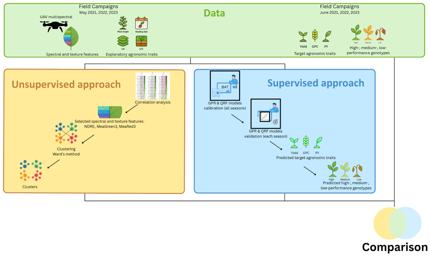
Building on these considerations, this study investigates supervised and unsupervised approaches based on UAV multispectral imagery for characterizing and grouping winter durum wheat genotypes according to grain yield, grain protein content (GPC), and protein yield (PY). In addition to grain yield and grain protein concentration, protein yield was evaluated because it integrates both traits and represents the total protein produced per unit area. As such, it is particularly relevant for breeding programs aiming to identify genotypes that combine high grain productivity with high grain protein production. A three-year field experiment was conducted in a breeding field comprising 26 genotypes, integrating ground measurements of yield and GPC with UAV imagery acquired at the end of flowering (BBCH 69) and the beginning of grain filling (BBCH 71). Two complementary approaches were evaluated. In the supervised approach, ML regression models were developed using UAV-derived SVIs, TFs, and additional phenotypic traits, including LAI, LCC, and canopy height, to predict the target traits. The predicted values were subsequently used to group genotypes into low-, medium-, and high-productivity classes. In the unsupervised approach, Ward’s clustering was applied directly to the UAV-derived SVIs and TFs to identify genotype groups without prior information on measured traits.

2. Materials and Methods

2.1. Test Site and Experimental Design of the Study

For this study, data were collected from a three-year plant breeding field trial at the Field Crops Institute, Chirpan (FCI–Chirpan), Bulgaria (Figure 1). The experimental fields were located in the Upper Thracian Plain on flat terrain with an altitude of 208–209 m a.s.l. The climate is temperate continental, with poorly expressed Mediterranean influence, and the soil is Pellic Vertisol. A competitive variety trial (CVT) with 26 genotypes of winter durum wheat (Triticum turgidum L. var. durum) was set up in the 2020–21, 2021–22 and 2022–23 growing seasons (referred to hereafter as the 2021, 2022, and 2023 seasons, respectively, for brevity). The CVT in 2022 was located approximately 300 m from the position of the CVTs in 2021 and 2023 (Figure 1). The genotypes included 24 breeding lines and the two varieties, Predel and Mirela, representing a standard. The experiment was a complete block design with four replications. Plot size was 13.2 m2 (12 × 1.10 m), the distance between the genotypes was 0.5 m, and between the replications was 2 m. The predecessor in all three seasons was winter peas, and the sowing rate was 550 germinated seeds per m2. The fields were sown on 6 November 2020, 12 November 2021, and 26 October 2022 and harvested on 15 July 2021, 11 July 2022, and 13 July 2023. Before sowing, 92 kg·ha−1 of active substance P2O5 was applied. Plants were supplied with 100 kg·ha−1 of nitrogen in February. The fields were treated with a combination of the herbicides Axial 050 EK (Syngenta, Basel, Switzerland) (900 mL·ha−1) and Biatlon 4 D (BASF, Ludwigshafen, Germany) (50 g·ha−1). No pesticides were employed for disease or pest control. In 2021, brown rust, yellow rust, and leaf spot pathogens caused by Septoria leaf blotch (STB) were observed at very low density on 27 May in genotype Mirela. In 2023, diseases were registered in all plots on 26 May: 23 genotypes were affected by yellow rust, all genotypes were affected by powdery mildew, and 24 genotypes were affected by STB.

2.2. Data Acquisition

2.2.1. Ground-Measured Data

Two field campaigns (FCs) were conducted within each growing season. The first FC for each season was conducted in late May, during the End of Flowering (BBCH 69, [41]) and Watery Ripe (BBCH 71, [41]) phenophases of the winter wheat genotypes—when the first grains have reached half of their final size. The second FC took place in July, at the agronomic maturity phenophase.
During the first FC of each season, measurements of plant height, Leaf Area Index (LAI), and Leaf Chlorophyll Content (LCC) were carried out. Plant height was measured in all 104 plots (26 genotypes in four replications). The height from the soil surface to the end of the spike (without the awns) on the main stem of 20 plants was measured in each plot and averaged. LAI and LCC were measured only in the first and second replications of each genotype (a total of 52 plots). The LAI measurements were carried out using the instrument AccuPAR LP-80 (METER Group, Inc., Pullman, WA, USA). A total of 10 measurements were made, evenly distributed across the plot, providing more representative information about the vegetation canopy. The plants’ LCC was measured using the CCM-300 (Opti-Sciences, Inc., Hudson, NH, USA) instrument. This instrument was used to measure the middle of the flag leaf blade of four representative plants selected in the middle of the plot. These measurements were then averaged at the plot level. The Heading Date (HD), defined as the number of days from 1 January to heading, was recorded when more than 50% of the plants within a plot reached the BBCH 59 growth stage. Before harvest, the number of productive tillers per plant was recorded.
During the second FC of each season, yield (kg per plot) data were collected. Harvesting was performed at the plot level using a standard plot combine harvester. The harvested grain from each plot was weighed under laboratory conditions using an electronic scale to determine yield per plot. To determine the Grain Protein Content (GPC), three randomly selected subsamples were taken from each plot and the results were averaged. Protein content was determined using the Kjeldahl method (N × 5.7) in accordance with BDS EN ISO 20483: 2013 [42], with modifications developed at FCI–Chirpan. A detailed description of this procedure is provided in our previous study [43]. Based on the measured yield (kg per plot) and GPC (%) data, the protein yield (PY, kg protein per plot) was calculated using the following equation:
P Y = ( y i e l d × G P C ) / 100

2.2.2. UAV Data and Spectral and Texture Features

UAV data were collected during the first FC of each growing season (Table 1). High-resolution multispectral imagery of the experimental fields was acquired using a Phantom 4 Multispectral (P4M) quadcopter (SZ DJI Technology Co., Ltd., Shenzhen, China). The system captures five spectral bands: Near-Infrared (NIR, 840 nm ± 26 nm), Red Edge (RE, 730 nm ± 16 nm), Red (R, 650 nm ± 16 nm), Green (G, 560 nm ± 16 nm), and Blue (B, 450 nm ± 16 nm). The UAV is equipped with an integrated sunlight irradiance sensor that records downwelling irradiance at the same wavelengths (https://ag.dji.com/p4-multispectral, accessed on 19 March 2026), enabling the derivation of surface reflectance during post-processing without the need for radiometric calibration targets [44]. Flights were conducted under clear sky conditions at a height of 50 m above ground, resulting in a ground sampling distance of approximately 2.6 cm. Four Ground Control Points (GCPs), located at the corners of the experimental fields, were measured using a GS08 GNSS receiver (Leica, Wetzlar, Germany) in RTK mode and used to improve the georeferencing of the mosaics. Image mosaicking was performed using the Pix4Dmapper v4.10. software (https://pix4d.com, accessed on 19 March 2026).
To achieve the objectives of the study, we selected 22 SVIs from the large number commonly used in precision agriculture and crop breeding (Appendix A: Table A1). These indices were chosen based on their reported strong correlations with the agronomic traits, such as yield [9,16,17,21,23,24,25,45,46,47,48,49,50,51,52], GPC [21,30,43,49,53], and PY [43,53,54], as well as their reliance on blue, green, red, red-edge, and near-infrared spectral bands.
We derived eight Grey Level Co-occurrence Matrix (GLCM)-based TFs [55]: Contrast (Con), Dissimilarity (Dis), Homogeneity (Hom), Angular Second Moment (ASM), Entropy (Ent), Mean (Mea), Variance (Var), and Correlation (Cor). Characterizing image texture using GLCM measures is one of the most widely used approaches for incorporating texture information into remote sensing image analysis. For a detailed description and the corresponding mathematical formulations of these features, the reader is referred to Hall-Beyer’s work [56]. Texture features were computed for each of the five spectral bands using three window sizes (3, 5, and 7 pixels), resulting in a total of 8 × 5 × 3 = 120 features. Before texture extraction, the input bands were quantized to 16 gray levels using an equal probability quantization approach, which generates bins containing approximately equal numbers of samples [55,57]. All texture measures were made directionally invariant by averaging across four orientations (horizontal, vertical, and the two diagonal directions), with a fixed spatial displacement of one pixel. The shifting distance was set to 1 pixel. The analysis was performed using the R package GLCMTextures [57]. For convenience, short names of the TFs were used throughout the manuscript, for example, EntRE3 denotes the entropy texture measure derived from the red-edge (RE) band using a 3-pixel window, where the prefix indicates the texture measure, the band abbreviation specifies the spectral band, and the suffix indicates the window size.
For each plot, the SVIs and TFs were computed by averaging pixel values within manually digitized plot boundaries. A 30 cm buffer was applied to exclude boundary effects and mixed pixels along plot edges. In addition, within-plot heterogeneities, such as gaps in the crop canopy caused by sowing irregularities or weed presence, were removed from the analysis. Finally, the four replications were averaged to obtain representative genotype-level values.

2.3. Data Analysis

This study used two methods, unsupervised and supervised, to group genotypes into three performance groups (low, medium, and high) with respect to the target agronomic traits: yield, GPC, and PY. Both methods used the UAV-based SVIs and TFs for this purpose. The unsupervised method included two steps: first, the best SVIs and TFs were selected based on their correlations with the target traits; second, the genotypes were split into three clusters using cluster analysis applied to the selected SVI, TF, and SVI + TF. To test the eventual positive effect of using additional ground-measured canopy characteristics on the grouping, we performed separate analyses adding four “explanatory” agronomic traits (plant height, HD, LAI, and LCC) to the UAV features. The supervised method employed two ML algorithms to develop models to predict yield, GPC, and PY. All SVIs, TFs, and “explanatory” agronomic traits were used as potential predictors, leaving the ML algorithms to select the most relevant for the final model. The genotypes were then grouped into three performance groups based on the yield, GPC, and PY values predicted by the best model. The groups were defined based on the mean and standard deviation (SD) of the predicted values. The performance groupings of both unsupervised and supervised methods were compared and validated against groups defined based on the mean and SD of the ground-measured yield, GPC, and PY. ANOVA was used to show the significance of the genotype (G), environment (season) (E), and G × E effects on the target agronomic traits and the selected SVIs and TFs. The individual methods are described in the following subsections, and the overall workflow is presented in Figure 2.

2.3.1. Correlation Analysis

The relationships between the agronomic traits (yield, GPC, and PY) and UAV-derived features were assessed using Pearson’s correlation coefficient. A two-sided p-value of <0.05 was considered statistically significant. For each agronomic trait, UAV features showing significant correlation in at least two of the three seasons were identified. When multiple SVIs or TFs met this criterion, the feature with the highest overall correlation across the three seasons was selected. The resulting spectral and texture features were then used as inputs for the ANOVA and cluster analysis (see below).

2.3.2. Analysis of Variance (ANOVA)

The effects of genotype, growing season, and their interaction on the variation in the agronomic traits and the selected UAV features were assessed using a two-way analysis of variance (ANOVA). The total sum of squares (SS) represents the total variability in the data and is partitioned into components attributable to the main effects, their interaction, and residual error. The mean square (MS) is obtained by dividing the SS by its degrees of freedom and provides an estimate of variance for each source of variation. Effect size was quantified using eta-squared (η2), calculated as the ratio of the sum of squares for a given factor to the total sum of squares (SS_factor/SS_total), indicating the proportion of total variance explained by that factor. The ANOVA analysis was performed using Statistica 13.

2.3.3. Unsupervised Method (Cluster Analysis)

Agglomerative hierarchical clustering was used to determine potentially homogeneous groups of genotypes with respect to selected SVIs, TFs, and explanatory agronomic traits. The hierarchical clustering produces a tree-like graphical representation of the observations and their grouping, called a dendrogram [58]. The clustering starts by treating each observation as an individual cluster (a dendrogram “leaf”) and proceeds iteratively, fusing the two most similar clusters at each iteration. This continues until all of the observations belong to one single cluster (the “trunk” of the dendrogram) [58]. The clustering analysis was performed using R 4.1.1 [59]. The data were first centered and scaled by subtracting the mean and dividing by the SD. A distance matrix was computed using the Euclidean distance measure and the dist function. The hclust function was used for clustering, setting the method argument to “ward.D2”, which minimizes the within-group dispersion [60,61]. Three clusters were defined in each dendrogram to facilitate the comparison with high-, medium-, and low-performance categories determined from ground-measured yield, GPC, and PY (see below). The clustering analysis was performed for each season with four datasets—(i) selected SVIs, (ii) selected TFs, (iii) combined SVIs and TFs, and (iv) combined SVIs, TFs—and explanatory agronomic traits (plant height, HD, LAI, and LCC).

2.3.4. Supervised Method (Regression Analysis)

Two machine learning algorithms were employed to retrieve yield, GPC, and PY from UAV-based features and explanatory agronomic traits (plant height, HD, LAI, and LCC): Gaussian Process Regression (GPR) [62] and Quantile Regression Forest (QRF) [63,64]. Both approaches quantify predictive uncertainty, albeit through fundamentally different mechanisms: GPR derives uncertainty analytically from the posterior predictive distribution, whereas QRF estimates it empirically via conditional quantiles from an ensemble of decision trees.
Both models were implemented using the MATLAB version 2024b-based ARTMO v3.3.2 (Automated Radiative Transfer Models Operator) toolbox [65]. The GPR was configured using an Automatic Relevance Determination (ARD) Rational Quadratic kernel. The QRF model was implemented as an ensemble of 200 regression trees (NTrees = 200), each trained on the full training dataset. At each split, all predictor variables were considered for node partitioning (NvarToSample = 100%), and the minimum number of observations per terminal node was set to five (MinLeaf = 5) to control tree complexity and reduce overfitting.
A single model was trained using the combined dataset from all three growing seasons. The dataset was randomly divided into training (70%) and independent validation (30%) subsets. The training subset contained 55 samples, and the independent validation set contained 23 samples. Model calibration was carried out using the training dataset, while the independent validation subset was used for performance assessment. To improve model robustness, bare soil samples were included in the training dataset. These samples were used exclusively for model calibration and were not included in the validation dataset. Model robustness and generalization ability were assessed using a three-fold cross-validation (CV) procedure applied to the training data. A feature selection procedure was carried out using the Band Analysis Tool (BAT) [66] within the ARTMO framework to determine the most informative predictors while reducing input dimensionality. The method assessed the contribution of individual predictors to model performance and identified an optimal subset of features that preserved predictive accuracy with a minimal number of inputs.
Model performance was evaluated on both the training set (with cross-validation) and validation datasets using the coefficient of determination (R2), root mean square error (RMSE), and normalized RMSE (nRMSE). The best-performing model was applied to the complete dataset for each growing season to evaluate its ability to accurately retrieve yield, GPC, and PY under season-specific conditions. These metrics were computed as follows:
R 2 = 1 i = 1 n ( V i o b s V i e s t ) 2 i = 1 n ( V i o b s V ¯ o b s ) 2
R M S E = 1 n i = 1 n ( V i e s t V i o b s ) 2
n R M S E = R M S E R a n g e ( V o b s )
where V i o b s is the observed value, V i e s t is the estimated value, V ¯ o b s is the mean of the observed values, n is the number of samples, and R a n g e ( V o b s ) is the maximal minus the minimal observed value.
As the regression method provides quantitative data rather than genotype groups, the predicted values were classified into low-, medium-, and high-performance groups using the Mean ± 1 Standard Deviation (SD) for each trait. Genotypes with predicted values greater than Mean + 1 SD were classified as high performers, those with values lower than Mean − 1 SD as low performers, and those within the interval Mean ± 1 SD as medium performers.

2.3.5. Methods Evaluation

The performance of the supervised and unsupervised approaches was evaluated by comparing their genotype classifications with those obtained from ground-measured yield, GPC, and PY. The reference groups were generated from the ground measurements using the same Mean ± 1 SD classification scheme described above. We then calculated what percentage of genotypes in each group were correctly identified by both methods. The performance groups from the supervised method could be directly compared with those from the ground-measured data as they were determined based on the same principle. For the unsupervised method, we studied the genotypes in each cluster to identify the best match to the ground-data-based grouping. Results were reported only for the two extreme performance groups—low and high. We tested the significance of the difference in the percent of correctly identified genotypes by the two methods using the exact McNemar test [67]. The exact McNemar test uses the binomial distribution rather than a chi-squared statistic and is more appropriate for small samples as in this study. The mcnemar function from the statsmodels v0.10.1 package [68] in Python v3.7.3 was used to perform the test.

3. Results

3.1. Meteorological Conditions and Agronomic Traits

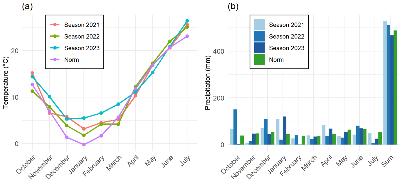
Figure 3 shows the monthly mean air temperature and monthly precipitation for the three seasons, compared with the multi-year norm for the period 1928–2023, for the Chirpan synoptic station of the National Institute of Meteorology and Hydrology located in close proximity to the breeding field. The three growing seasons were significantly warmer than the multi-year norm. The warmest season was 2023, exceeding the multi-year temperature sum by 23 degrees, followed by 2021 and 2022, which exceeded it by 13 and 9 degrees, respectively. The average temperature during the winter months (December to February) was significantly higher than the multi-year norm for all three growing seasons, while temperatures from March to June were generally around the norm. The only exception was March 2023, when the average monthly temperature exceeded the norm by 2.8 °C. In July of all three growing seasons, higher temperatures than the multi-year norm were recorded (Figure 3a).
Annual precipitation was above the multi-year norm in the first two growing seasons, by 42 mm in 2021 and 23 mm in 2022, but below the norm by 20 mm in 2023 (Figure 3b). In all three seasons, monthly precipitation was more unevenly distributed compared to the multi-year norm. In the first two seasons, precipitation in October and December significantly exceeded the norm, while precipitation in November was significantly lower. In the third season, October precipitation was significantly below the multi-year norm, while November and December precipitation were around the norm. January precipitation in 2021 and 2023 exceeded the multi-year norm by approximately 2.5 times, and February 2023 had extremely low precipitation. March precipitation was somewhat consistent with the multi-year norm across the three growing seasons, while April rainfall exceeded the norm in 2021 and 2023. May rainfall was below the multi-year norm across all three seasons, with 2022 having the lowest. June rainfall in 2022 and 2023 was above normal, while July rainfall across all growing seasons was below the multi-year norm for 1928–2023.
The meteorological conditions during the growing seasons of 2021 and 2022 were similar, favorably affecting the development, productivity, and quality of winter durum wheat grain. Optimal grain yield was observed under the meteorological conditions of the first season (2021), whereas protein content was maximized under the meteorological conditions of the second season (2022). Protein yield was similarly high in both seasons. Higher temperatures and lower precipitation characterized the 2023 growing season compared to the multi-year norm. Despite favorable meteorological conditions for biomass development, the resulting yield and protein content were low. This outcome was most likely caused by the severe foliar disease outbreak observed in May.
When observing the condition of winter durum wheat genotypes across the three flight missions (FMs), both similarities and differences are evident, depending on the agronomic traits studied. During all FMs, only minor differences in the phenological development of winter durum wheat genotypes were observed (Table 1). During FM1, the genotypes were distributed across two phenological phases, BBCH 69 and BBCH 71, with 69% at BBCH 69. The same phenological phases were observed during FM3 in May 2023, but with the opposite distribution. In contrast, no differences were recorded during FM2, as all genotypes were at BBCH 71. During FM1, plant diseases were observed at very low density, whereas during FM3, all plots showed symptoms of disease infection. No plant diseases were detected during FM2 in May 2022.
Substantial differences were observed in plant height and LAI among the three growing seasons (Table 2). In 2022, plants were approximately 14–16 cm shorter than in the other two seasons. In contrast, LAI values in 2023 were 1.5–1.8 times higher than those recorded in 2021 and 2022. This increase was likely associated not only with plant height but also with a greater number of productive tillers per plant.
The average LCC values varied within relatively narrow ranges across all three seasons (Table 2). The difference between the lowest measured LCC value (recorded in 2023) and the highest value (recorded in 2021) was only 31 mg·m−2.
The yield, GPC, and PY recorded in 2021 and 2022 showed no substantial difference (Table 2). In contrast, significantly lower values for all three agronomic traits were observed in 2023. Compared with 2021, the yield and PY in 2023 were lower by 3.86 kg/plot and 0.66 kg protein/plot, respectively. In addition, the GPC in 2023 was 2.8% lower than the maximum value recorded in 2022 (Table 2).
Differences in the heading date (HD) among the studied genotypes ranged from 7 to 11 days, depending on the growing season. Mean HD values across all breeding lines exhibited only minor interannual variation, differing by one to three days over the three years. The coefficients of variation for HD were consistently low, indicating that it was the most stable trait across growing seasons compared with the other traits studied. In the first and second seasons, the average HD values differed by only 1 day, with genotype variation ranging from 139 to 146/147 days. The earliest average heading was observed in 2023, when the range among genotypes was wider, varying from 133 to 144 days.
Overall, the results of the field campaigns indicate a general similarity in the measured agronomic traits between the first and second growing seasons, except for plant height. In contrast, the 2023 season was characterized by the lowest yield, GPC, and PY values, despite exhibiting the greatest plant height and the highest number of productive tillers per plant. During the third flight mission (FM3), high LAI values were recorded, and disease symptoms were observed in all plots. In general, the evaluated traits showed relatively low variability among genotypes, as reflected by the low coefficients of variation (CVs) across all three seasons. Slightly higher CV values were observed in 2023 for LAI, yield, and PY, as well as for productive tiller numbers in 2021 and LAI in 2022 (Table 2).

3.2. Yield, GPC, and PY Correlations with UAV Features

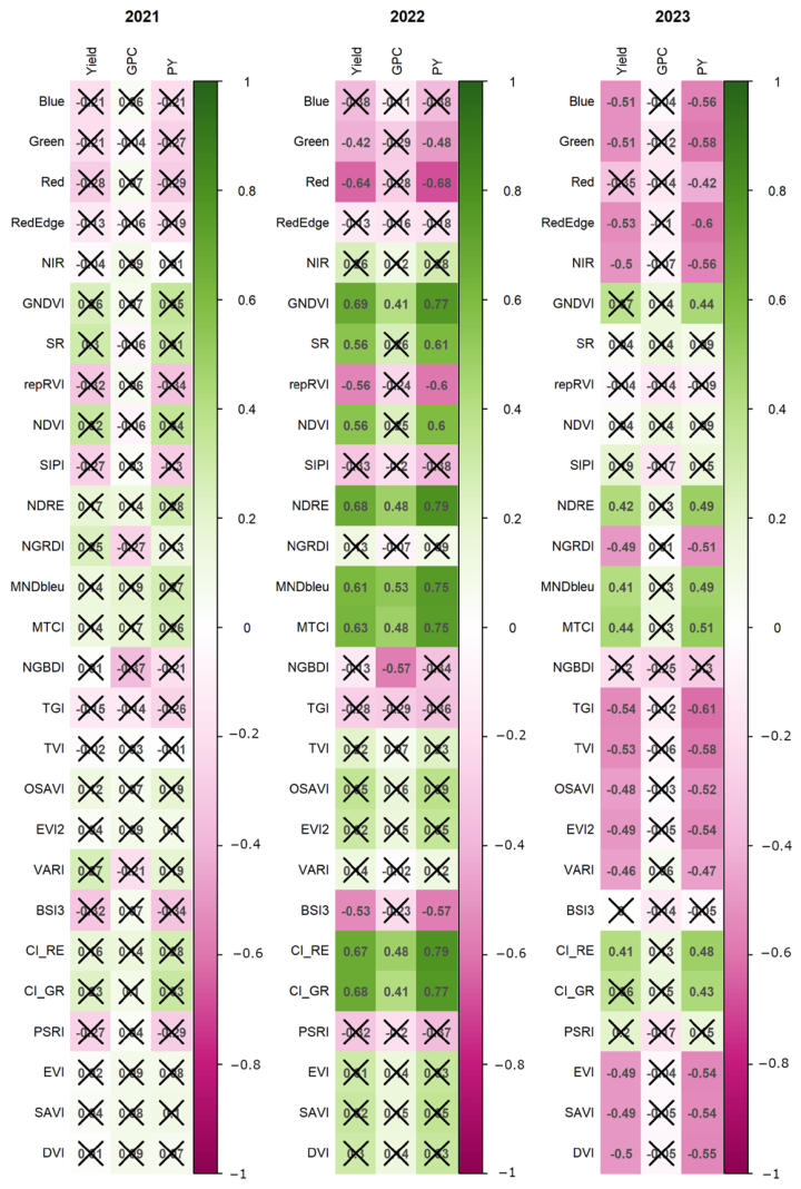
The correlations between spectral bands, SVIs, and agronomic traits (yield, GPC, and PY) are presented in Appendix A, Figure A1. In 2023, yield and PY showed significant correlations with most spectral features, with the strongest relationships observed for TGI (−0.54 and −0.61, respectively). In 2022, most spectral features were not significantly correlated with yield or PY; however, some individual indices, such as GNDVI and NDRE, exhibited relatively strong correlations (0.69 and 0.79, respectively). In 2021, no significant correlations were found between any spectral features and either yield or PY. GPC showed no significant correlation with any spectral features in 2021 and 2023 and was significantly correlated with only a limited number of SVIs in 2022, with NGBDI showing the strongest relationship (−0.57).
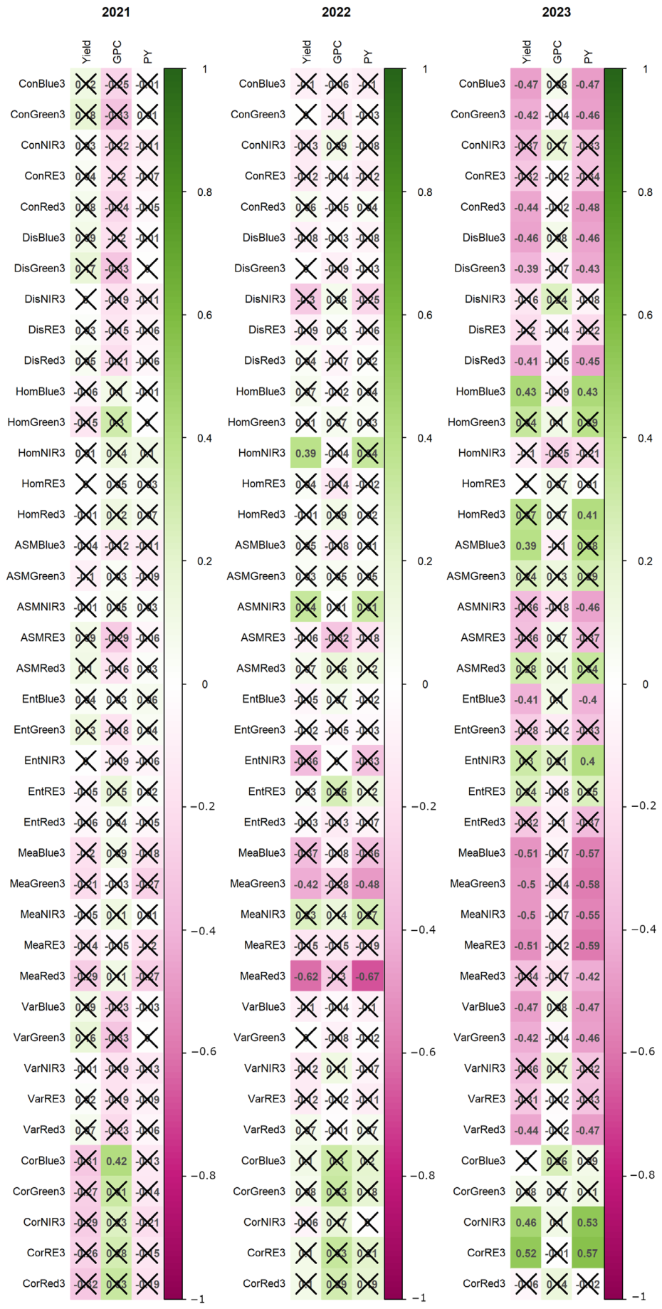
The correlations between TFs and agronomic traits are presented in Appendix A, Figure A2, with results reported for the 3 × 3 window size. Correlation patterns for the 5 × 5 and 7 × 7 window sizes were nearly identical to those obtained with the 3 × 3 window, indicating that the smallest window was sufficient to capture the relevant spatial information. Increasing the window size did not provide additional explanatory value, likely due to the correspondence between the pixel size (2.6 cm) and the scale of canopy elements such as leaves and spikes. In 2023, approximately half of the TFs were significantly correlated with yield and PY, with maximum absolute correlation values comparable to those for SVIs for the same season (|0.52| and |0.59|, respectively). In contrast, no significant correlations were observed in 2021, and only a few were detected in 2022. GPC showed no significant relationship with TFs except for a single case (CorBlue3) in 2021.
Overall, the strength and consistency of relationships between agronomic traits and UAV features were strongly season-dependent, and the performance of most features varied considerably across years. Table 3 summarizes the spectral and texture features that showed significant correlations with each agronomic trait in at least two seasons. No feature met this criterion for GPC, and none of the features were consistently significant across all three seasons for either yield or PY. Among the SVIs, NDRE exhibited the strongest and most consistent correlations with both yield and PY. Among the TFs, MeaGreen3 and MeaRed3 were selected as the most representative for yield and PY, respectively (Table 3).

3.3. ANOVA

Analysis of variance (Table 4) revealed that genotype, environment (growing season), and their interactions had a statistically significant influence on the variation in the studied agronomic traits and the selected UAV features (NDRE, MeaGreen3, and MeaRed3), except for NDRE, which was not significantly influenced by the interaction term. The growing season accounted for the largest proportion of variation in yield (η2 = 82.1%), GPC (η2 = 86.5%), and PY (η2 = 88.8%). Similarly, it was the dominant source of variation in NDRE (η2 = 69.1%). In contrast, genotype exerted a stronger influence on the variation in MeaGreen3 (η2 = 56.3%) and MeaRed3 (η2 = 35.1%).

3.4. Unsupervised Method

We conducted a clustering analysis of the studied genotypes for each season using the selected UAV features (NDRE, MeaGreen3, and MeaRed3), both individually and in combination with the explanatory agronomic traits LAI, LCC, plant height, and HD to identify potentially homogeneous groups of genotypes. We examined the correspondence between the genotype clusters and the performance groupings based on ground-measured data. In particular, we examined whether high- and low-performing genotypes were separated into distinct clusters or whether they were mixed within the same cluster. The results are presented in Appendix A, Table A2.
When comparing the two grouping approaches, we observed that the degree of overlap between genotype groups and clusters varied depending on the agronomic trait, UAV features, their combinations, and the growing season.
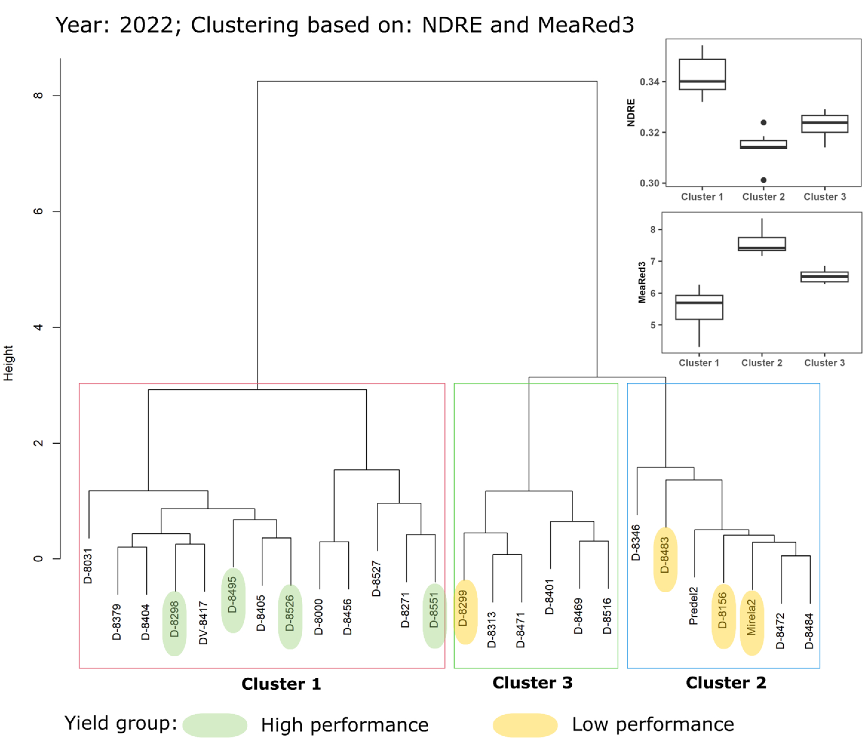
For yield, the highest agreement between performance groups (high- and low-yielding genotypes) and clustering results across all three seasons was obtained when clustering was based on the combined use of the spectral index NDRE and the texture feature MeaRed3. The best performance was achieved in 2022, when 100% of the high-yielding genotypes were assigned to cluster 1, while 75% of the low-yielding genotypes were assigned to cluster 2 (Appendix A: Figure A3). In 2022 and 2023, a relatively high degree of overlap between performance groups and clusters was also observed when using MeaRed3 alone and the combination of NDRE and MeaGreen3. Across all growing seasons, high-yielding genotypes within the same cluster were consistently characterized by higher NDRE and lower MeaRed3 values, whereas low-yielding genotypes exhibited lower NDRE and higher MeaRed3 values.
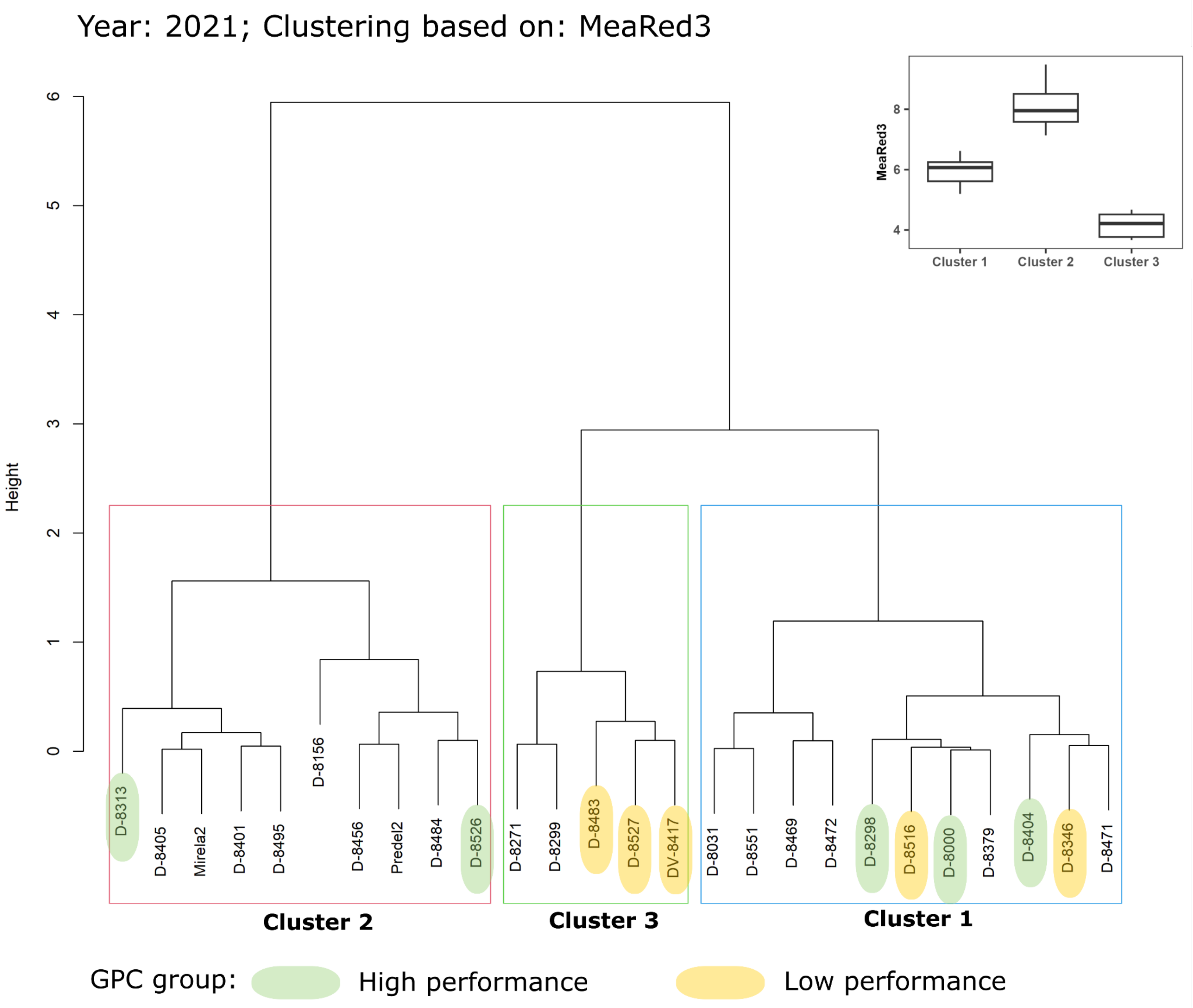
Regarding GPC, separating high- and low-performance genotypes into distinct clusters was most successful when using MeaRed3 across all three seasons. The highest degree of agreement between performance groups and clustering results was observed in 2021 (Appendix A: Figure A4).
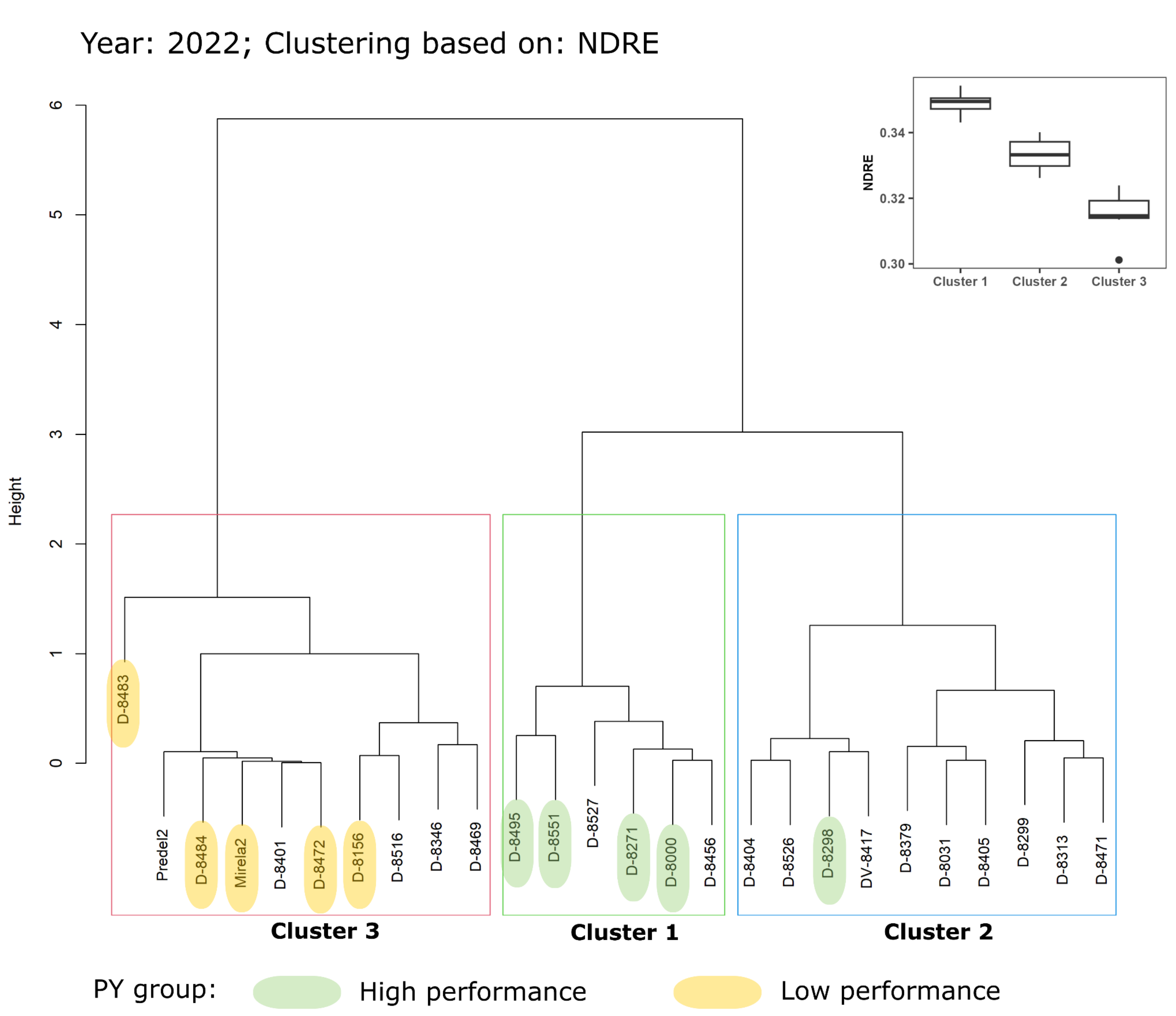
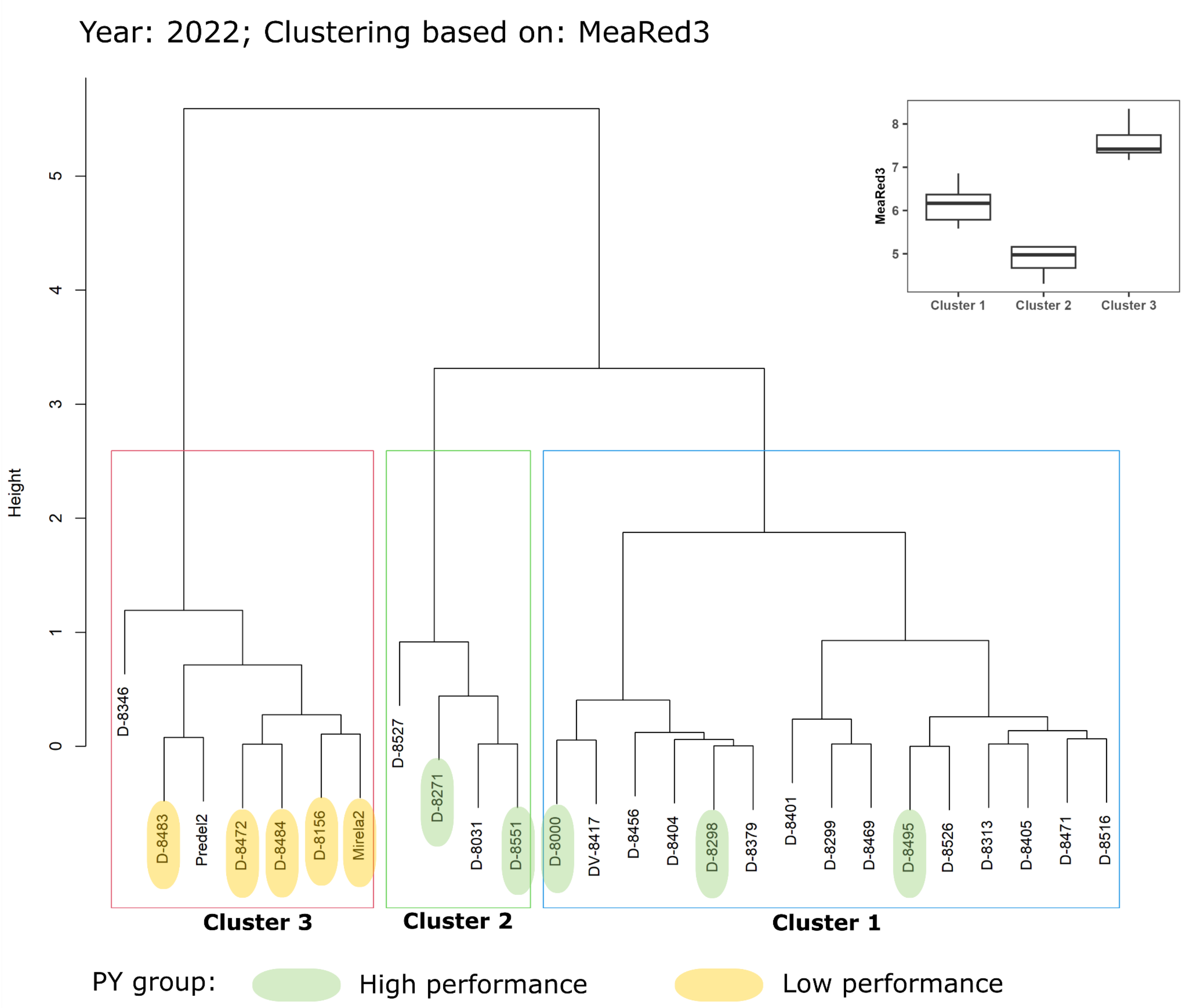
In terms of PY, the highest percentage of genotypes from both groups (high-yielding and low-yielding) in all three seasons fell into two different clusters when clustering was performed based on either NDRE or MeaRed3. The best results were again obtained in 2022: For NDRE, 80% of high-performance genotypes fell into cluster 1 and 100% of low-performance ones into cluster 3 (Appendix A: Figure A5). For MeaRed3, 60% of high-performance genotypes fell into cluster 1 and 100% of low-performance ones into cluster 3 (Appendix A: Figure A6, Table A2). The highest percentage of overlap of genotypes between high- and low-performance groups and clusters was achieved with the combination of NDRE and MeaRed3, but only for one season—2022. Across all growing seasons, high-performance PY genotypes that fall into a single cluster are distinguished by higher NDRE and lower MeaRed3, whereas low-yielding genotypes have lower NDRE and higher MeaRed3.
Overall, the degree of overlap between performance groups and clusters was unsatisfactory for all studied agronomic traits when clustering was based on the combined set of SVIs, TFs, and explanatory agronomic traits. In this case, using six variables for clustering resulted in highly heterogeneous clusters.
Across all seasons, the clusters containing the majority of high- and low-performing genotypes also included a substantial number of genotypes with medium performance, indicating limited separability between the defined groups.

3.5. Supervised Method

The performance metrics of the best-performing models, derived from the training set (n = 55) and independent validation set (n = 23), are reported in Table 5. Relevant predictor features were selected using the Band Analysis tool. Overall, all models demonstrated strong predictive performance, as indicated by the high cross-validation and independent validation R2 values. Among the evaluated algorithms, the QRF model exhibited the most consistent performance between cross-validation and independent validation, suggesting greater robustness and generalization capability.
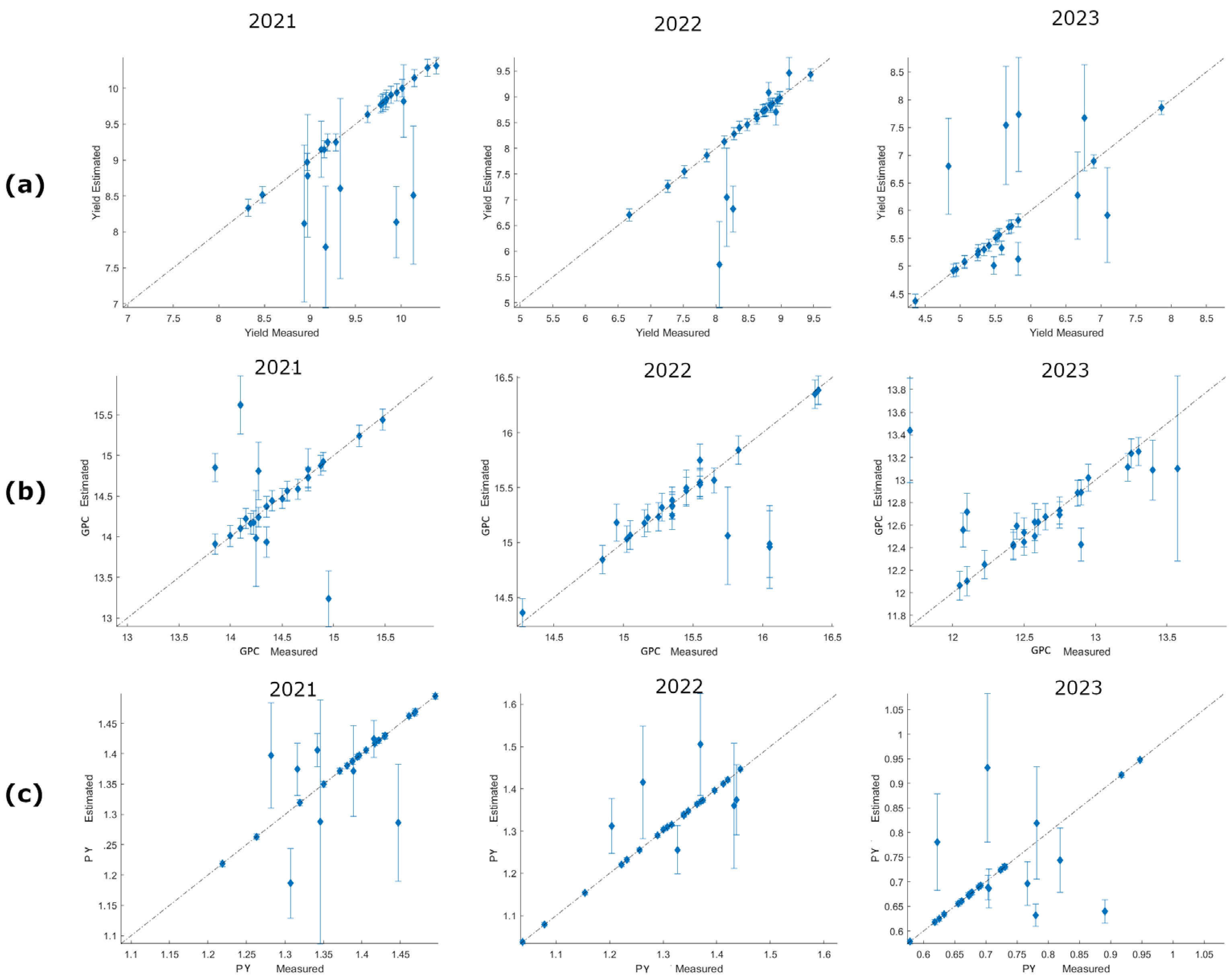
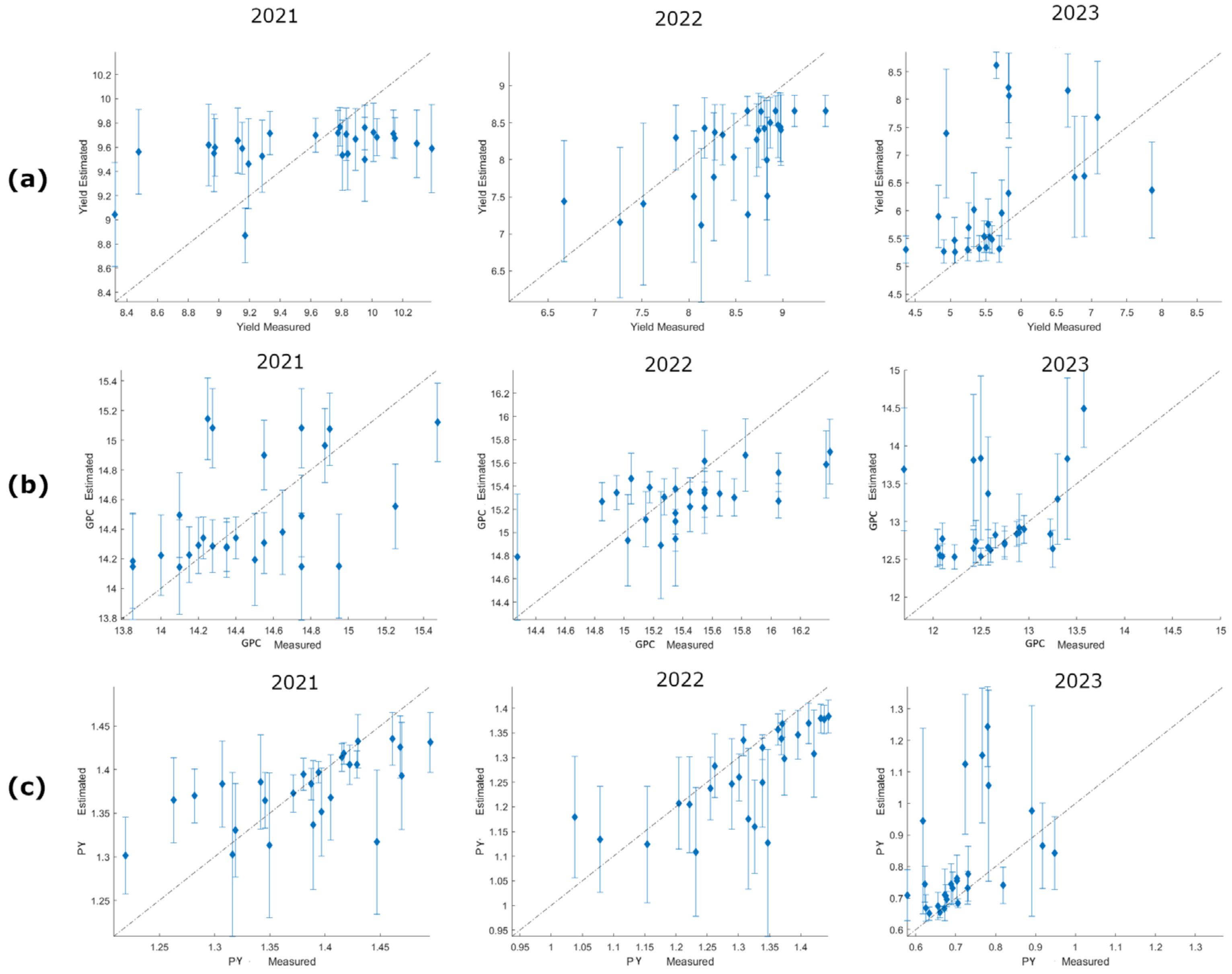
The models reported in Table 5 were applied to the complete dataset for each year to evaluate their robustness and predictive performance across diverse environmental conditions. The resulting year-specific performance metrics are presented in Table 6 and Appendix A (Figure A7 and Figure A8). When the models were applied to the complete dataset on a season-by-season basis, the GPR models generally outperformed the QRF models, despite QRF showing superior performance when evaluated using the combined three-year dataset. Across both modeling algorithms, predictive performance was highest in 2022, whereas lower accuracies were observed in 2021 and 2023.
The performance of the supervised approach was evaluated by comparing genotype classifications derived from the GPR models with those obtained from ground measurements (Appendix A: Table A2 and Table A3). Only GPR models with season-specific predictive performance of R2 ≥ 0.45 (Table 6) were considered for genotype grouping.
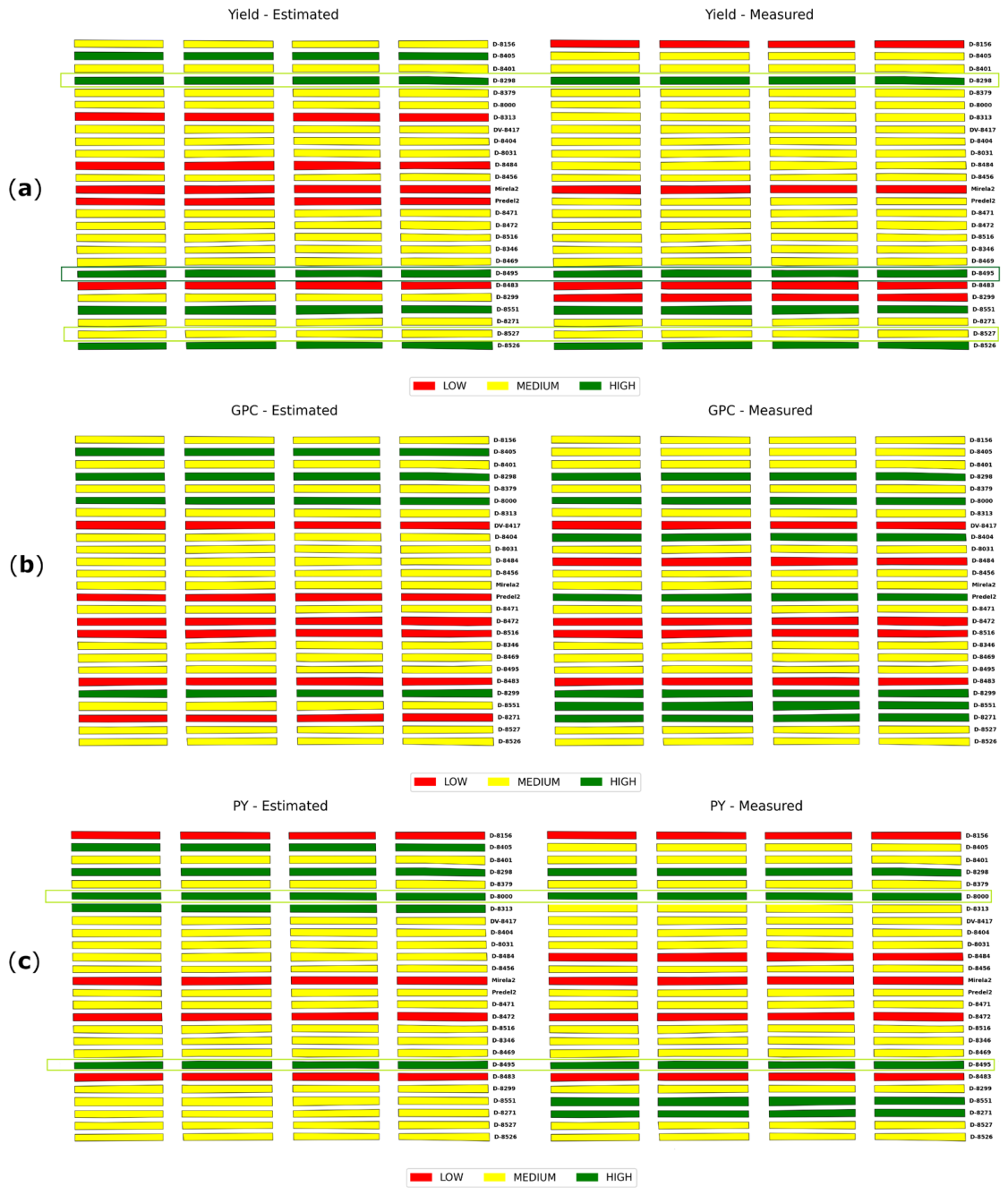
Genotype-level comparison (Appendix A: Table A3, Figure A9) showed good agreement between measured and predicted performance groups. For yield, all four genotypes predicted as high-yielding in 2021 were included in the measured high-yielding group, while four of the seven predicted low-yielding genotypes also belonged to the measured low-yielding group. In 2022, four of the five predicted high-yielding genotypes matched the measured classification, whereas agreement for the low-yielding group was lower, with two common genotypes. Measured data confirmed three of the six genotypes predicted to belong to the high-yielding group and all three genotypes predicted to belong to the low-yielding group in 2023.
For GPC, genotype-level comparison was performed only for 2022. Three of the four predicted high-GPC genotypes were included in the measured high-GPC group, while four of the six predicted low-GPC genotypes were included in the measured low-GPC group.
For PY, strong agreement between measured and predicted classifications was observed in both evaluated seasons. In 2021, field measurements confirmed that all four genotypes predicted to belong to the high-performing group did so, as did all four genotypes predicted to belong to the low-performing group. In 2022, three of the five predicted high-performing genotypes and all four predicted low-performing genotypes agreed with the measured classifications.
Several breeding lines showed stable performance across seasons according to both field measurements and model predictions. Breeding line D-8495 consistently belonged to the high-yielding group in all three seasons, while D-8527 and D-8298 were classified as high-yielding in two seasons. For protein yield, D-8000 and D-8495 were consistently identified as high-performing genotypes across the two growing seasons.
Overall, the supervised approach successfully identified between 43% and 100% of the high- and low-performing genotypes, depending on the agronomic trait, growing season, and performance group (Appendix A: Table A2). The highest classification accuracy was achieved for yield, reaching 100% for the high-yielding group in 2022, whereas the lowest accuracy (43%) was obtained for the high-GPC group in the same season. Classification of PY was generally more consistent than GPC, with accuracies ranging from 60% to 80% for both high- and low-performing groups.

4. Discussion

4.1. Environment and Genotype Influence

The ANOVA results in Table 4 reveal significant, but distinct, influences of genotypes, environments, and their interactions on the variation in the studied agronomic traits and remote-sensing-derived features. Environmental conditions explained the highest percentage of the estimated total variation for yield, GPC, PY, and NDRE, highlighting that environmental conditions across the three growing seasons differed, affecting overall genotype performance. This also explains the significantly smaller effects of genotype and interaction on agronomic traits that we found. The predominant influence of environmental conditions on yield and GPC aligns with results from many previous studies across different durum wheat genotypes and environments/locations. The sensitivity of canopy reflectance and physiological traits to environmental drivers such as temperature and water availability explains the large effect of growing seasons on NDRE variation, which can substantially modify relationships with agronomic traits across years.
In contrast, TFs derived from the green and red bands (MeaGreen3 and MeaRed3) showed a stronger genotype effect, suggesting that these metrics may capture structurally controlled canopy characteristics, such as plant architecture or spatial canopy organization. However, these texture features exhibited high residual error. Further examination indicated that Replicate 4 presented markedly different values compared to the other replicates, substantially increasing the within-genotype variance.
The divergence observed in Replicate 4 may be attributed to localized micro-environmental conditions (e.g., soil heterogeneity or moisture gradients), differences in plant density or lodging, or image-acquisition factors such as illumination, shadowing, or minor geometric misalignment. Because texture metrics rely on spatial pixel relationships, they are inherently more sensitive to small-scale variations than vegetation indices. Consequently, although texture features may better reflect genotype-specific structural traits, their stability appears more susceptible to replicate-level variability and acquisition conditions.
The results of the analysis of variance explain the inconsistency across seasons. The same genotypes, especially high-yielding ones, express their genetic potential differently across the agronomic traits studied in response to the distinct meteorological conditions prevailing in each season. This makes it difficult to conduct an objective breeding assessment using both ground measurements and UAV features in a single season. Nevertheless, genotypes with high and stable yield potential across two or three seasons were identified through both ground measurements and remote-sensing-derived features.

4.2. Temporal Generalization and Season-Dependent Performance of the Regression Models

Although the models trained on the pooled three-season dataset achieved moderate to high cross-validation performance (R2 = 0.71–0.86; Table 5), this did not consistently translate into temporal generalization under season-specific conditions (Table 6). Cross-validation variability also differed among models, with GPR Yield (R2 = 0.76 ± 0.05) and GPR GPC (R2 = 0.86 ± 0.04) showing relatively stable performance across folds, whereas QRF models (R2 SD = 0.20–0.28) and GPR PY (R2 = 0.85 ± 0.14) exhibited greater variability. These findings indicate that mean cross-validation performance alone does not fully describe model robustness and may provide optimistic estimates of predictive ability when samples from contrasting environmental conditions are randomly mixed.
Cross-validation on pooled multi-season data assumes exchangeability among samples, an assumption that is violated by substantial interannual variability in meteorological and phenological conditions. Consequently, the models captured relationships that performed well under mixed-condition sampling but were less transferable across growing seasons. This was reflected by a systematic reduction in predictive performance when the models were applied to individual years, particularly in 2021 and 2023 compared with 2022.
The relatively small number of training samples (n = 55) compared with the initial number of candidate predictors may also have affected the stability of feature selection. To mitigate this risk, feature selection was performed using the Band Analysis Tool (BAT) separately within each cross-validation training fold, thereby preventing information leakage from the validation data and reducing the dimensionality of the predictor space before model calibration. The different feature subsets selected for GPR and QRF are expected, as the two algorithms rely on different learning principles and optimization criteria. Consequently, the selected variables should be interpreted as model-specific predictor combinations rather than universally optimal feature sets.
The 2023 season was characterized by low yield and protein content (Table 2), which were overestimated by the regression models (Appendix A: Figure A7a,c). This indicates that the factors that negatively affected yield did not manifest in the UAV features at the end of the flowering and the beginning of the grain-filling phase. The possible effects of the disease outbreak in 2023 were analyzed in this context. Yellow rust, powdery mildew, and STB-infected wheat typically show reduced NIR reflectance and increased reflectance in the visible region [69,70,71,72]. However, exceptions from the general rule were observed in previous studies. Gui et al. [70] found no significant difference in visible-region reflectance between healthy and yellow rust-infected wheat. They explained this by the localized nature of the chlorosis, which affected only parts of the leaves. Yu et al. [72] found practically no difference in the spectra of STB-infected and healthy wheat in the early stages (end of May). Therefore, the infestation in 2023 may have affected the final yield but was not detectable in BBCH 69–71. Unfortunately, disease assessment was limited to recording disease occurrence (presence/absence), and no quantitative scoring of disease severity or incidence was performed. Therefore, it was not possible to directly analyze or quantify the effects of individual diseases on canopy reflectance or texture features. Disease occurrence and environmental stress are both known to influence canopy reflectance and texture characteristics. Foliar diseases such as yellow rust, powdery mildew, and STB reduce green leaf area and chlorophyll content, thereby increasing reflectance in the visible region and altering vegetation indices. Similarly, heat and drought stress accelerate senescence, reduce canopy water content, and modify canopy structure, resulting in measurable changes in spectral signatures and image texture. Since disease severity and physiological stress indicators were not quantified in the present study, their individual effects could not be separated. Consequently, the observed UAV-derived traits likely reflect the combined influence of genotype, disease occurrence, and environmental stress.
The highest predictive consistency was observed in 2022, when the GPR achieved R2 ≥ 0.53 across all traits, suggesting a more stable relationship between spectral features and genotype responses. In contrast, the lower performance observed in 2021 and 2023 is consistent with genotype × environment interactions altering the spectral–trait relationships. These results highlight the importance of explicit temporal validation and environment-aware modeling strategies for improving the robustness of multi-season phenotyping models.
Several studies have reported nonlinear relationships between UAV-derived features, yield, and GPC [43,73]. However, how these relationships vary across environments and how they influence protein content prediction remain poorly understood [73].
In the present study, PY consistently showed higher predictive performance than yield and GPC in season-specific analyses, suggesting that it may represent a more robust target for multi-year modeling. Because the PY integrates both biomass production and grain protein concentration, it may be less sensitive to year-to-year variability affecting each component individually.

4.3. Performance of the Supervised and Unsupervised Methods

In this study, correlations between agronomic traits and UAV-derived features varied among seasons, highlighting the challenge of predicting crop performance using remote sensing under contrasting environmental conditions. The fluctuating correlations between traits across environments are well-documented in plant breeding, highlighting the complex, polygenic nature of crop adaptation. This instability in trait relationships is mainly due to genotype-by-environment interaction, resulting in distinct phenotypes for the same genotype under specific growing conditions. Nevertheless, the NDRE and the texture features, MeaGreen3 and MeaRed3, showed significant correlations (p < 0.05) with yield and PY in at least two seasons (Table 3; Appendix A: Figure A1 and Figure A2) and were used to identify homogeneous genotype groups through an unsupervised approach. In parallel, measured genotype performance groups for yield, GPC, and PY were defined based on the mean and standard deviation of ground observations. Comparison between UAV-based clustering and ground-based classification revealed substantial overlap among genotype groups, although the agreement depended on the trait, UAV feature combination, and growing season. The selected UAV features were particularly effective for distinguishing high- and low-performing genotypes for yield and PY. High-yielding genotypes generally showed higher NDRE and lower MeaRed3 values at the end of flowering and the beginning of grain filling, whereas low-yielding genotypes exhibited the opposite trend. The positive relationship between NDRE and yield is consistent with NDRE as an indicator of chlorophyll content, nitrogen status, and canopy vigor [74]. Conversely, lower MeaRed3 values are associated with reduced red reflectance caused by chlorophyll absorption in healthy, dense canopies [75].
For GPC, MeaRed3 provided the strongest separation between high- and low-performing genotypes. However, the agreement between UAV-derived clusters and measured GPC groups was weaker than for yield and PY, likely due to the limited correlations between GPC and the evaluated UAV features. This differs from the results of Tan et al. [76], who reported a strong relationship between GPC and NDVI in winter wheat. The discrepancy may be explained by the narrower range of GPC values among the genotypes investigated in the present study (Table 2), which reduced the ability to detect subtle differences among genotypes.
The results support previous findings highlighting the value of texture information for crop phenotyping. Consistent with Kang et al. [12], the GLCM Mean (Mea) texture metric showed a strong association with grain yield. Previous studies [12,13] have also demonstrated that integrating spectral and textural features improves the characterization of wheat phenotypic variability and enhances yield prediction accuracy. The results of the present study further confirm this finding.
The results demonstrate that UAV-derived spectral and texture features acquired at the end of flowering and beginning of grain filling can support the identification of high- and low-performing genotypes in breeding trials, particularly for yield and PY. Although the performance of this approach varied among seasons, UAV-based phenotyping provides a cost-effective strategy for screening large numbers of genotypes and reducing the need for extensive biometric measurements and repeated harvesting.
The supervised method further confirmed the potential of UAV-based phenotyping for genotype evaluation. The agreement between measured and model-derived performance groups varied among traits and seasons, reflecting differences in model predictive ability. The highest agreement was obtained for yield in 2022, when the modeled high-performing genotype group fully matched the measured group, demonstrating the supervised model’s ability to identify superior genotypes under favorable prediction conditions.
The supervised and unsupervised approaches showed comparable performance in distinguishing high- and low-performance genotypes across traits and seasons, with each method outperforming the other in specific cases. However, no consistent superiority of either approach was observed. This was confirmed by McNemar’s test, which detected no statistically significant differences in classification accuracy between the two methods for any trait or growing season (Appendix A: Table A2). However, the unsupervised method provided results in each case. In contrast, the supervised method could not be applied when the regression models had low predictive performance, as was the case with GPC in 2021 and 2023 and PY in 2023. This indicates that when an accurate regression model is missing, the unsupervised method is the only alternative. Apart from accuracy, the utility of the two methods may depend on the use case, as they require different processing steps and may be applied in different situations. The supervised approach provides quantitative predictions of agronomic traits and enables direct genotype ranking; however, it requires a calibrated model developed from representative training data and is therefore dependent on model availability and transferability. The unsupervised method is easier to implement and does not require prior model development, but cluster interpretation requires additional ground information to associate groups with high- or low-performing genotypes. Moreover, it provides only relative performance information within a specific season rather than quantitative estimates of agronomic traits.

4.4. Future Work

The presented results highlight the strong influence of inter-annual variability on the applicability of UAV data and suggest that universal models across growing seasons may be difficult to achieve without explicitly incorporating environmental covariates. Integrating meteorological variables (e.g., temperature, precipitation), soil moisture indicators, or phenology-related parameters may help disentangle season-specific effects and improve model transferability. Alternatively, developing season-specific calibration models or adopting hierarchical or domain-adaptation approaches could enhance robustness in multi-season phenotyping studies. Additionally, future studies should investigate hybrid approaches that combine the complementary strengths of supervised and unsupervised methods, supported by larger multi-environment datasets, to improve the robustness, transferability, and scalability of UAV-based phenotyping for breeding applications. Future studies should also evaluate the stability of the selected predictor subsets across repeated resampling schemes and compare BAT with alternative feature-selection methods that explicitly account for predictor redundancy, using larger multi-environment datasets.

5. Conclusions

Pre-harvest identification of high- and low-yielding genotypes using UAV data has the potential to improve the efficiency of field breeding trials and reduce phenotyping cost. This study evaluated spectral and texture features extracted from multispectral UAV images at the end of flowering and the beginning of grain filling to identify durum wheat genotypes showing high or low yield, GPC, and PY using unsupervised and supervised methods. Both approaches successfully identified high- and low-performing genotypes for yield and PY, achieving accuracies of 50–100%. Relatively low performance was shown for GPC, highlighting the stronger influence of seasonal variability and the limited spectral expression of differences in protein content.
The ANOVA results supported the regression findings by demonstrating the dominant influence of environmental conditions on agronomic traits and NDRE, which contributed to reduced temporal transferability of predictive models. In contrast, texture features showed greater ability to capture genotype-related structural characteristics; however, they require careful interpretation due to their sensitivity to spatial noise and replicate-level anomalies. Future research should consider implementing normalization procedures and replicate-level quality-control diagnostics to enhance the robustness and stability of texture-derived features.
The regression results emphasize that validation across pooled multi-season data may not fully reflect real-world temporal transferability. Explicit consideration of environmental variability is critical when developing operational remote-sensing-based prediction models. Among the evaluated traits, PY showed the most consistent predictability, suggesting that integrated traits combining yield and quality components may provide more robust targets for UAV-based phenotyping across diverse growing conditions.

Author Contributions

Conceptualization, E.R. and V.B.; methodology, V.B., D.G., E.R. and P.D.; formal analysis, D.G., P.D. and R.D.; investigation, R.D., K.T. and S.N.; data curation, D.G., R.D. and P.D.; writing—original draft preparation, D.G., E.R., V.B. and P.D.; writing—review and editing, D.G., E.R., V.B. and P.D.; visualization, P.D. and D.G.; supervision, E.R.; project administration, D.G.; funding acquisition, V.B. and E.R. All authors have read and agreed to the published version of the manuscript.

Funding

This research was funded by project BG16RFPR002-1.014-0012-C01, Establishment and sustainable development of a Center of Competence “Agrifood Systems and Bioeconomy”, financed by the European Regional Development Fund through the “Program for Research, Innovation and Digitalisation for Smart Transformation” (PRIDST).

Data Availability Statement

The raw data supporting the conclusions of this article will be made available by the authors on request.

Acknowledgments

We express our gratitude to the Bulgarian Ministry of Education and Science for the support of the National Research Programme “Smart Crop Production” (approved by the Ministry Council Decision N◦ 866/26 November 2020). The field and UAV data used in this publication were collected under this program. This article is supported by the EU COST (European Cooperation in Science and Technology) Action CA22136 ‘Pan-European Network of Green Deal Agriculture and Forestry Earth Observation Science’ (PANGEOS). The authors used ChatGPT (version GPT-5; OpenAI, San Francisco, CA, USA) to improve the manuscript’s readability, grammar, and clarity. The authors reviewed, edited, and verified all generated text and took full responsibility for the content of the publication.

Conflicts of Interest

The authors declare no conflicts of interest. The funders had no role in the design of the study; in the collection, analyses, or interpretation of data; in the writing of the manuscript; or in the decision to publish the results.

Appendix A

Table A1. Spectral vegetation indices used in the study. In the formulas, ρ_i is the reflectance, and λ_i is the central wavelength (nm) of the spectral band labeled i (see Section 2.2.2 for band names and corresponding central wavelengths).
Vegetation IndexFormulaReference
Simple ratio (SR)ρ_NIR/ρ_R[77]
Normalized difference vegetation index (NDVI)(ρ_NIR − ρ_R)/(ρ_NIR + ρ_R)[78]
Green normalized difference vegetation index (GNDVI)(ρ_NIR − ρ_G)/(ρ_NIR + ρ_G)[79]
Reciprocal ratio vegetation index (repRVI)ρ_R/ρ_NIR[77]
Structure-insensitive pigment index (SIPI)(ρ_NIR − ρ_B)/(ρ_NIR − ρ_R)[80]
Normalized difference red-edge index (NDRE)(ρ_NIR − ρ_RE)/(ρ_NIR + ρ_RE)[81]
Difference vegetation index (DVI)ρ_NIR − ρ_R[82]
Normalized green–red difference index (NGRDI)(ρ_G − ρ_R)/(ρ_G + ρ_R)[82]
Normalized green–blue difference index (NGBDI)(ρ_G − ρ_B)/(ρ_G + ρ_B)[83]
Modified normalized difference blue index (mNDblue)(ρ_B − ρ_RE)/(ρ_B + ρ_NIR)[84]
MERIS terrestrial chlorophyll index (MTCI)(ρ_NIR − ρ_RE)/(ρ_RE − ρ_R)[85]
Triangular greenness index (TGI)−0.5 × [(λ_R − λ_B) × (ρ_R − ρ_G)−(λ_R − λ_G) × (ρ_R − ρ_B)][86]
Triangular vegetation index (TVI)0.5 × [(λ_R − λ_G) × (ρ_NIR − ρ_G)−(λ_NIR − λ_G) × (ρ_R − ρ_G)][87]
Soil adjusted vegetation index (SAVI)1.5 × (ρ_NIR − ρ_R)/(ρ_NIR + ρ_R + 0.5)[88]
Optimized soil adjusted vegetation index (OSAVI)(ρ_NIR − ρ_R)/(ρ_NIR + ρ_R + 0.16)[89]
Enhanced vegetation index (EVI)2.5 × (ρ_NIR − ρ_R)/(ρ_NIR + 6×ρ_R − 7.5 × ρ_B + 1)[90]
2-band enhanced vegetation index (EVI2)2.5 × (ρ_NIR − ρ_R)/(ρ_NIR + 2.4 × ρ_R + 1)[91]
Visible atmospherically resistant index (VARI)(ρ_G − ρ_R)/(ρ_G + ρ_R − ρ_B)[92]
3-band vegetation index (3BSI-Tian)(ρ_R − ρ_NIR − ρ_G)/(ρ_R + ρ_NIR + ρ_G)[17,93]
Plant senescence reflectance index (PSRI)(ρ_R − ρ_B)/ρ_NIR[94]
Green chlorophyll index (CIgreen)ρ_NIR/ρ_G − 1[95]
Red-edge chlorophyll index (CIred-edge)ρ_NIR/ρ_RE − 1[95]
Table A2. Percentages of high- and low-performance genotypes correctly identified using supervised and unsupervised methods. The asterisk indicates unsatisfactory regression model performance for a particular year and trait, preventing the implementation of the supervised method.
TraitYearPerformance GroupCorrectly Identified by Supervised Method (%)Correctly Identified by Unsupervised Method (%)McNemar’s Test Significance 1
Yield2021High66.750ns
Low8080ns
2022High100100ns
Low5075ns
2023High6080ns
Low5050ns
GPC2021High*60-
low*60-
2022High4357ns
Low8060ns
2023High*40-
low*60-
PY2021High8060ns
Low8080ns
2022High6060ns
Low80100ns
2023High*75-
Low*75-
1 ns: not significant at the 0.05 level of significance.
Table A3. Comparison of the measured and predicted high- and low-performing genotype groups based on the GPR models. Accordingly, n represents the number of genotypes included in each performance group.
TraitSeasonPerformance GroupMeasured Genotypes (n; Value Range)Predicted Genotypes (n; Value Range)Common Genotypes (n)Common Genotypes
Yield2021High6;
10.0–10.4
4;
10.0–10.3
4Predel
D-8469
D-8483
D-8495
Yield2021Low5;
8.3–8.98
7;
8.1–8.88
4D-8313
D-8484 Mirela
D-8526
Yield2022High4;
8.98–9.45
5;
8.98–9.46
4D-8298
D-8495
D-8526
D-8551
Yield2022Low4;
6.67–7.52
5;
5.74–7.3
2Mirela2
D-8483
Yield2023High5;
6.67–7.86
6;
6.87–7.86
3D-8031
D-8298
D-8527
Yield2023Low6;
4.36–5.06
3;
4.37–4.9
3D-8484
D-8456
D-8526
GPC2022High7;
15.7–16.4
4;
15.8–16.4
3D-8298
D-8000
D-8299
GPC2022Low5;
14.3–15.05
6;
14.4–15.06
4DV-8417
D-8472
D-8483
D-8516
PY2021High5;
1.45–1.49
4;
1.43–1.5
4D-8000
D-8379
D-8495
Predel
PY2021Low5;
1.22–1.32
6;
1.19–1.3
4D-8156
D-8313
D-8456
D-8484
PY2022High5;
1.41–1.5
5;
1.4–1.51
3D-8000
D-8298
D-8495
PY2022Low5;
1.08–1.22
4;
1.03–1.22
4D-8156
D-8472
D-8483
Mirela2
Figure A1. Pearson’s correlation coefficients of the spectral bands and vegetation indices with the agronomic traits yield, grain protein content (GPC), and protein yield (PY). Insignificant correlations (p > 0.05) are marked with ×.
Remotesensing 18 02664 g0a1
Figure A2. Pearson’s correlation coefficients of the texture features with the agronomic traits yield, grain protein content (GPC), and protein yield (PY). Insignificant correlations (p > 0.05) are marked with ×.
Remotesensing 18 02664 g0a2
Figure A3. Dendrogram of genotypes clustered based on NDRE and MeaRed3 in 2022 showing the distribution of high- and low-yield genotypes within the three clusters. The boxplots show the distribution of NDRE and MeaRed3 in the clusters.
Remotesensing 18 02664 g0a3
Figure A4. Dendrogram of genotypes clustered based on MeaRed3 in 2021 showing the distribution of high- and low-GPC genotypes within the three clusters. The boxplot shows the distribution of MeaRed3 in the clusters.
Remotesensing 18 02664 g0a4
Figure A5. Dendrogram of genotypes clustered based on NDRE in 2022 showing the distribution of high- and low-PY genotypes within the three clusters. The boxplot shows the distribution of NDRE in the clusters.
Remotesensing 18 02664 g0a5
Figure A6. Dendrogram of genotypes clustered based on MeaRed3 in 2022 showing the distribution of high- and low-PY genotypes within the three clusters. The boxplot shows the distribution of MeaRed3 in the clusters.
Remotesensing 18 02664 g0a6
Figure A7. Agreement between the measured and model-predicted agronomic traits across the 2021–2023 growing seasons using the GPR models: (a) Yield; (b) GPC; (c) PY. The dashed line represents the 1:1 line.
Remotesensing 18 02664 g0a7
Figure A8. Agreement between the measured and model-predicted agronomic traits across the 2021–2023 growing seasons using the QRF models: (a) Yield; (b) GPC; (c) PY. The dashed line represents the 1:1 line.
Remotesensing 18 02664 g0a8
Figure A9. Comparison of genotype groupings based on measured and GPR-predicted agronomic traits in 2022: (a) yield, (b) grain protein content (GPC), and (c) protein yield (PY). Genotypes consistently identified as high-performing across all three years are shown in dark green, while those identified as high-performing in two of the three years are shown in light green.
Remotesensing 18 02664 g0a9

References

  1. Grosse-Heilmann, M.; Cristiano, E.; Deidda, R.; Viola, F. Durum Wheat Productivity Today and Tomorrow: A Review of Influencing Factors and Climate Change Effects. Resour. Environ. Sustain. 2024, 17, 100170. [Google Scholar] [CrossRef]
  2. Xynias, I.N.; Mylonas, I.; Korpetis, E.G.; Ninou, E.; Tsaballa, A.; Avdikos, I.D.; Mavromatis, A.G. Durum Wheat Breeding in the Mediterranean Region: Current Status and Future Prospects. Agronomy 2020, 10, 432. [Google Scholar] [CrossRef]
  3. Jeon, D.; Kang, Y.; Lee, S.; Choi, S.; Sung, Y.; Lee, T.-H.; Kim, C. Digitalizing Breeding in Plants: A New Trend of next-Generation Breeding Based on Genomic Prediction. Front. Plant Sci. 2023, 14, 1092584. [Google Scholar] [CrossRef] [PubMed]
  4. Herr, A.W.; Adak, A.; Carroll, M.E.; Elango, D.; Kar, S.; Li, C.; Jones, S.E.; Carter, A.H.; Murray, S.C.; Paterson, A.; et al. Unoccupied Aerial Systems Imagery for Phenotyping in Cotton, Maize, Soybean, and Wheat Breeding. Crop Sci. 2023, 63, 1722–1749. [Google Scholar] [CrossRef]
  5. Gano, B.; Bhadra, S.; Vilbig, J.M.; Ahmed, N.; Sagan, V.; Shakoor, N. Drone-based Imaging Sensors, Techniques, and Applications in Plant Phenotyping for Crop Breeding: A Comprehensive Review. Plant Phenome J. 2024, 7, e20100. [Google Scholar] [CrossRef]
  6. Tanaka, T.S.T.; Wang, S.; Jørgensen, J.R.; Gentili, M.; Vidal, A.Z.; Mortensen, A.K.; Acharya, B.S.; Beck, B.D.; Gislum, R. Review of Crop Phenotyping in Field Plot Experiments Using UAV-Mounted Sensors and Algorithms. Drones 2024, 8, 212. [Google Scholar] [CrossRef]
  7. Reynolds, M.; Chapman, S.; Crespo-Herrera, L.; Molero, G.; Mondal, S.; Pequeno, D.N.L.; Pinto, F.; Pinera-Chavez, F.J.; Poland, J.; Rivera-Amado, C.; et al. Breeder Friendly Phenotyping. Plant Sci. 2020, 295, 110396. [Google Scholar] [CrossRef] [PubMed]
  8. Camenzind, M.P.; Yu, K. Multi Temporal Multispectral UAV Remote Sensing Allows for Yield Assessment across European Wheat Varieties Already before Flowering. Front. Plant Sci. 2024, 14, 1214931. [Google Scholar] [CrossRef] [PubMed]
  9. Zhou, M.; Zheng, H.; He, C.; Liu, P.; Awan, G.M.; Wang, X.; Cheng, T.; Zhu, Y.; Cao, W.; Yao, X. Wheat Phenology Detection with the Methodology of Classification Based on the Time-Series UAV Images. Field Crops Res. 2023, 292, 108798. [Google Scholar] [CrossRef]
  10. Radočaj, D.; Šiljeg, A.; Marinović, R.; Jurišić, M. State of Major Vegetation Indices in Precision Agriculture Studies Indexed in Web of Science: A Review. Agriculture 2023, 13, 707. [Google Scholar] [CrossRef]
  11. Chang-Brahim, I.; Koppensteiner, L.J.; Beltrame, L.; Bodner, G.; Saranti, A.; Salzinger, J.; Fanta-Jende, P.; Sulzbachner, C.; Bruckmüller, F.; Trognitz, F.; et al. Reviewing the Essential Roles of Remote Phenotyping, GWAS and Explainable AI in Practical Marker-Assisted Selection for Drought-Tolerant Winter Wheat Breeding. Front. Plant Sci. 2024, 15, 1319938. [Google Scholar] [CrossRef] [PubMed]
  12. Kang, Y.; Wang, Y.; Fan, Y.; Wu, H.; Zhang, Y.; Yuan, B.; Li, H.; Wang, S.; Li, Z. Wheat Yield Estimation Based on Unmanned Aerial Vehicle Multispectral Images and Texture Feature Indices. Agriculture 2024, 14, 167. [Google Scholar] [CrossRef]
  13. Liu, L.; Zhou, X.; Liu, T.; Liu, D.; Liu, J.; Wang, J.; Yi, Y.; Zhu, X.; Zhang, N.; Zhang, H.; et al. Characterizing Growth and Estimating Yield in Winter Wheat Breeding Lines and Registered Varieties Using Multi-Temporal UAV Data. Agriculture 2025, 15, 2554. [Google Scholar] [CrossRef]
  14. Gracia-Romero, A.; Kefauver, S.C.; Fernandez-Gallego, J.A.; Vergara-Díaz, O.; Nieto-Taladriz, M.T.; Araus, J.L. UAV and Ground Image-Based Phenotyping: A Proof of Concept with Durum Wheat. Remote Sens. 2019, 11, 1244. [Google Scholar] [CrossRef]
  15. Naser, M.; Khosla, R.; Longchamps, L.; Dahal, S. Using NDVI to Differentiate Wheat Genotypes Productivity Under Dryland and Irrigated Conditions. Remote Sens. 2020, 12, 824. [Google Scholar] [CrossRef]
  16. Liu, J.; Zhu, Y.; Tao, X.; Chen, X.; Li, X. Rapid Prediction of Winter Wheat Yield and Nitrogen Use Efficiency Using Consumer-Grade Unmanned Aerial Vehicles Multispectral Imagery. Front. Plant Sci. 2022, 13, 1032170. [Google Scholar] [CrossRef] [PubMed]
  17. Ganeva, D.; Roumenina, E.; Dimitrov, P.; Gikov, A.; Jelev, G.; Dragov, R.; Bozhanova, V.; Taneva, K. Phenotypic Traits Estimation and Preliminary Yield Assessment in Different Phenophases of Wheat Breeding Experiment Based on UAV Multispectral Images. Remote Sens. 2022, 14, 1019. [Google Scholar] [CrossRef]
  18. Li, Z.; Chen, Z.; Cheng, Q.; Duan, F.; Sui, R.; Huang, X.; Xu, H. UAV-Based Hyperspectral and Ensemble Machine Learning for Predicting Yield in Winter Wheat. Agronomy 2022, 12, 202. [Google Scholar] [CrossRef]
  19. Prey, L.; Ramgraber, L.; Seidl-Schulz, J.; Hanemann, A.; Noack, P.O. The Transferability of Spectral Grain Yield Prediction in Wheat Breeding across Years and Trial Locations. Sensors 2023, 23, 4177. [Google Scholar] [CrossRef] [PubMed]
  20. Fei, S.; Hassan, M.A.; Xiao, Y.; Su, X.; Chen, Z.; Cheng, Q.; Duan, F.; Chen, R.; Ma, Y. UAV-Based Multi-Sensor Data Fusion and Machine Learning Algorithm for Yield Prediction in Wheat. Precis. Agric. 2023, 24, 187–212. [Google Scholar] [CrossRef] [PubMed]
  21. Kaushal, S.; Gill, H.S.; Billah, M.M.; Khan, S.N.; Halder, J.; Bernardo, A.; Amand, P.S.; Bai, G.; Glover, K.; Maimaitijiang, M.; et al. Enhancing the Potential of Phenomic and Genomic Prediction in Winter Wheat Breeding Using High-Throughput Phenotyping and Deep Learning. Front. Plant Sci. 2024, 15, 1410249. [Google Scholar] [CrossRef] [PubMed]
  22. Yuan, J.; Zhang, Y.; Zheng, Z.; Yao, W.; Wang, W.; Guo, L. Grain Crop Yield Prediction Using Machine Learning Based on UAV Remote Sensing: A Systematic Literature Review. Drones 2024, 8, 559. [Google Scholar] [CrossRef]
  23. Heinemann, P.; Prey, L.; Hanemann, A.; Ramgraber, L.; Seidl-Schulz, J.; Noack, P.O. Enhancing Model Performance through Date Fusion in Multispectral and RGB Image-Based Field Phenotyping of Wheat Grain Yield. Precis. Agric. 2025, 26, 20. [Google Scholar] [CrossRef]
  24. Rufo, R.; Soriano, J.M.; Villegas, D.; Royo, C.; Bellvert, J. Using Unmanned Aerial Vehicle and Ground-Based RGB Indices to Assess Agronomic Performance of Wheat Landraces and Cultivars in a Mediterranean-Type Environment. Remote Sens. 2021, 13, 1187. [Google Scholar] [CrossRef]
  25. Guo, J.; Zeng, X.; Ma, Q.; Yuan, Y.; Zhang, N.; Lin, Z.; Yin, P.; Yang, H.; Liu, X.; Zhang, F. UAV-Based Yield Prediction Based on LAI Estimation in Winter Wheat (Triticum Aestivum L.) Under Different Nitrogen Fertilizer Types and Rates. Plants 2025, 14, 1986. [Google Scholar] [CrossRef] [PubMed]
  26. Volpato, L.; Pinto, F.; González-Pérez, L.; Thompson, I.G.; Borém, A.; Reynolds, M.; Gérard, B.; Molero, G.; Rodrigues, F.A. High Throughput Field Phenotyping for Plant Height Using UAV-Based RGB Imagery in Wheat Breeding Lines: Feasibility and Validation. Front. Plant Sci. 2021, 12, 591587. [Google Scholar] [CrossRef] [PubMed]
  27. Gracia-Romero, A.; Rufo, R.; Gómez-Candón, D.; Soriano, J.M.; Bellvert, J.; Yannam, V.R.R.; Gulino, D.; Lopes, M.S. Improving In-Season Wheat Yield Prediction Using Remote Sensing and Additional Agronomic Traits as Predictors. Front. Plant Sci. 2023, 14, 1063983. [Google Scholar] [CrossRef] [PubMed]
  28. Zhang, B.; Gu, L.; Dai, M.; Bao, X.; Sun, Q.; Zhang, M.; Qu, X.; Li, Z.; Zhen, W.; Gu, X. Estimation of Grain Filling Rate of Winter Wheat Using Leaf Chlorophyll and LAI Extracted from UAV Images. Field Crops Res. 2024, 306, 109198. [Google Scholar] [CrossRef]
  29. Yan, J.; Wang, X. Unsupervised and Semi-supervised Learning: The next Frontier in Machine Learning for Plant Systems Biology. Plant J. 2022, 111, 1527–1538. [Google Scholar] [CrossRef] [PubMed]
  30. Wolters, S.; Söderström, M.; Piikki, K.; Börjesson, T.; Pettersson, C.-G. Predicting Grain Protein Concentration in Winter Wheat (Triticum Aestivum L.) Based on Unpiloted Aerial Vehicle Multispectral Optical Remote Sensing. Acta Agric. Scand. Sect. B Soil Plant Sci. 2022, 72, 788–802. [Google Scholar] [CrossRef]
  31. Li, Z.; Zhao, Y.; Taylor, J.; Gaulton, R.; Jin, X.; Song, X.; Li, Z.; Meng, Y.; Chen, P.; Feng, H.; et al. Comparison and Transferability of Thermal, Temporal and Phenological-Based in-Season Predictions of above-Ground Biomass in Wheat Crops from Proximal Crop Reflectance Data. Remote Sens. Environ. 2022, 273, 112967. [Google Scholar] [CrossRef]
  32. Zhang, S.; Duan, J.; Qi, X.; Gao, Y.; He, L.; Liu, L.; Guo, T.; Feng, W. Combining Spectrum, Thermal, and Texture Features Using Machine Learning Algorithms for Wheat Nitrogen Nutrient Index Estimation and Model Transferability Analysis. Comput. Electron. Agric. 2024, 222, 109022. [Google Scholar] [CrossRef]
  33. Zheng, H.; Ji, W.; Wang, W.; Lu, J.; Li, D.; Guo, C.; Yao, X.; Tian, Y.; Cao, W.; Zhu, Y.; et al. Transferability of Models for Predicting Rice Grain Yield from Unmanned Aerial Vehicle (UAV) Multispectral Imagery across Years, Cultivars and Sensors. Drones 2022, 6, 423. [Google Scholar] [CrossRef]
  34. Garriga, M.; Romero-Bravo, S.; Estrada, F.; Escobar, A.; Matus, I.A.; Del Pozo, A.; Astudillo, C.A.; Lobos, G.A. Assessing Wheat Traits by Spectral Reflectance: Do We Really Need to Focus on Predicted Trait-Values or Directly Identify the Elite Genotypes Group? Front. Plant Sci. 2017, 8, 280. [Google Scholar] [CrossRef] [PubMed]
  35. Schirrmann, M.; Hamdorf, A.; Garz, A.; Ustyuzhanin, A.; Dammer, K.-H. Estimating Wheat Biomass by Combining Image Clustering with Crop Height. Comput. Electron. Agric. 2016, 121, 374–384. [Google Scholar] [CrossRef]
  36. Qin, W.; Wang, J.; Ma, L.; Wang, F.; Hu, N.; Yang, X.; Xiao, Y.; Zhang, Y.; Sun, Z.; Wang, Z.; et al. UAV-Based Multi-Temporal Thermal Imaging to Evaluate Wheat Drought Resistance in Different Deficit Irrigation Regimes. Remote Sens. 2022, 14, 5608. [Google Scholar] [CrossRef]
  37. Shen, L.; Deakin, G.; Ding, G.; Ali, M.; Dai, J.; Wen, Z.; Pinheiro, F.; Zhou, J.; Jackson, R. The Use of Low-Cost Drone and Multi-Trait Analysis to Identify High Nitrogen Use Lines for Wheat Improvement. Agronomy 2024, 14, 1612. [Google Scholar] [CrossRef]
  38. Marino, S.; Alvino, A. Detection of Homogeneous Wheat Areas Using Multi-Temporal UAS Images and Ground Truth Data Analyzed by Cluster Analysis. Eur. J. Remote Sens. 2018, 51, 266–275. [Google Scholar] [CrossRef]
  39. Marino, S.; Alvino, A. Agronomic Traits Analysis of Ten Winter Wheat Cultivars Clustered by UAV-Derived Vegetation Indices. Remote Sens. 2020, 12, 249. [Google Scholar] [CrossRef]
  40. Marino, S.; Alvino, A. Vegetation Indices Data Clustering for Dynamic Monitoring and Classification of Wheat Yield Crop Traits. Remote Sens. 2021, 13, 541. [Google Scholar] [CrossRef]
  41. Meier, U. Growth Stages of Mono- and Dicotyledonous Plants: BBCH Monograph; Julius Kühn-Institut: Quedlinburg, Germany, 2018. [Google Scholar] [CrossRef]
  42. ISO 20483:2013; Cereals and Pulses—Determination of the Nitrogen Content and Calculation of the Crude Protein Content—Kjeldahl Method. International Organization for Standardization: Geneva, Switzerland, 2013.
  43. Ganeva, D.; Roumenina, E.; Dimitrov, P.; Gikov, A.; Bozhanova, V.; Dragov, R.; Jelev, G.; Taneva, K. Preharvest Durum Wheat Yield, Protein Content, and Protein Yield Estimation Using Unmanned Aerial Vehicle Imagery and Pléiades Satellite Data in Field Breeding Experiments. Remote Sens. 2024, 16, 559. [Google Scholar] [CrossRef]
  44. Cubero-Castan, M.; Schneider-Zapp, K.; Bellomo, M.; Shi, D.; Rehak, M.; Strecha, C. Assessment of the Radiometric Accuracy in a Target Less Work Flow Using Pix4D Software. In Proceedings of the 2018 9th Workshop on Hyperspectral Image and Signal Processing: Evolution in Remote Sensing (WHISPERS); IEEE: Piscataway, NJ, USA, 2018; pp. 1–4. [Google Scholar]
  45. Wang, L.; Tian, Y.; Yao, X.; Zhu, Y.; Cao, W. Predicting Grain Yield and Protein Content in Wheat by Fusing Multi-Sensor and Multi-Temporal Remote-Sensing Images. Field Crops Res. 2014, 164, 178–188. [Google Scholar] [CrossRef]
  46. Kyratzis, A.C.; Skarlatos, D.P.; Menexes, G.C.; Vamvakousis, V.F.; Katsiotis, A. Assessment of Vegetation Indices Derived by UAV Imagery for Durum Wheat Phenotyping under a Water Limited and Heat Stressed Mediterranean Environment. Front. Plant Sci. 2017, 8, 1114. [Google Scholar] [CrossRef] [PubMed]
  47. Serrano, L.; Filella, I.; Peñuelas, J. Remote Sensing of Biomass and Yield of Winter Wheat under Different Nitrogen Supplies. Crop Sci. 2000, 40, 723–731. [Google Scholar] [CrossRef]
  48. Hassan, M.A.; Yang, M.; Rasheed, A.; Yang, G.; Reynolds, M.; Xia, X.; Xiao, Y.; He, Z. A Rapid Monitoring of NDVI across the Wheat Growth Cycle for Grain Yield Prediction Using a Multi-Spectral UAV Platform. Plant Sci. 2019, 282, 95–103. [Google Scholar] [CrossRef] [PubMed]
  49. Walsh, O.S.; Marshall, J.M.; Nambi, E.; Jackson, C.A.; Ansah, E.O.; Lamichhane, R.; McClintick-Chess, J.; Bautista, F. Wheat Yield and Protein Estimation with Handheld and Unmanned Aerial Vehicle-Mounted Sensors. Agronomy 2023, 13, 207. [Google Scholar] [CrossRef]
  50. Hassani, K.; Gholizadeh, H.; Taghvaeian, S.; Natalie, V.; Carpenter, J.; Jacob, J. Application of UAS-Based Remote Sensing in Estimating Winter Wheat Phenotypic Traits and Yield During the Growing Season. PFG—J. Photogramm. Remote Sens. Geoinf. Sci. 2023, 91, 77–90. [Google Scholar] [CrossRef]
  51. Tanabe, R.; Matsui, T.; Tanaka, T.S.T. Winter Wheat Yield Prediction Using Convolutional Neural Networks and UAV-Based Multispectral Imagery. Field Crops Res. 2023, 291, 108786. [Google Scholar] [CrossRef]
  52. Ali, N.; Mohammed, A.; Bais, A.; Berraies, S.; Ruan, Y.; Cuthbert, R.D.; Sangha, J.S. Field-Scale Precision: Predicting Grain Yield of Diverse Wheat Breeding Lines Using High-Throughput UAV Multispectral Imaging. IEEE J. Sel. Top. Appl. Earth Obs. Remote Sens. 2024, 17, 11419–11433. [Google Scholar] [CrossRef]
  53. Xue, L.-H.; Cao, W.-X.; Yang, L.-Z. Predicting Grain Yield and Protein Content in Winter Wheat at Different N Supply Levels Using Canopy Reflectance Spectra. Pedosphere 2007, 17, 646–653. [Google Scholar] [CrossRef]
  54. Dalla Marta, A.; Grifoni, D.; Mancini, M.; Orlando, F.; Guasconi, F.; Orlandini, S. Durum Wheat In-Field Monitoring and Early-Yield Prediction: Assessment of Potential Use of High Resolution Satellite Imagery in a Hilly Area of Tuscany, Central Italy. J. Agric. Sci. 2015, 153, 68–77. [Google Scholar] [CrossRef]
  55. Haralick, R.M.; Shanmugam, K.; Dinstein, I. Textural Features for Image Classification. IEEE Trans. Syst. Man Cybern. 1973, 6, 610–621. [Google Scholar] [CrossRef]
  56. Hall-Beyer, M. GLCM Texture: A Tutorial v. 3; University of Calgary: Calgary, AB, Canada, 2017. [Google Scholar]
  57. Ilich, A. GLCMTextures: GLCM Textures of Raster Layers; Zenodo: Geneva, Switzerland, 2025. [Google Scholar]
  58. James, G.; Witten, D.; Hastie, T.; Tibshirani, R. An Introduction to Statistical Learning with Applications in R, 1st ed.; Springer: Berlin/Heidelberg, Germany, 2013. [Google Scholar]
  59. R Core Team. R: A Language and Environment for Statistical Computing; R Foundation for Statistical Computing: Vienna, Austria, 2021. [Google Scholar]
  60. Ward, J.H. Hierarchical Grouping to Optimize an Objective Function. J. Am. Stat. Assoc. 1963, 58, 236–244. [Google Scholar] [CrossRef]
  61. Murtagh, F.; Legendre, P. Ward’s Hierarchical Agglomerative Clustering Method: Which Algorithms Implement Ward’s Criterion? J. Classif. 2014, 31, 274–295. [Google Scholar] [CrossRef]
  62. Rasmussen, C.E.; Williams, C.K.I. Gaussian Processes for Machine Learning; MIT Press: Cambridge, MA, USA, 2008. [Google Scholar]
  63. Breiman, L. Random Forests. Mach. Learn. 2001, 45, 5–32. [Google Scholar] [CrossRef]
  64. Meinshausen, N. Quantile Regression Forests. J. Mach. Learn. Res. 2006, 7, 983–999. [Google Scholar]
  65. Caicedo, J.P.R.; Verrelst, J.; Muñoz-Marí, J.; Moreno, J.; Camps-Valls, G. Toward a Semiautomatic Machine Learning Retrieval of Biophysical Parameters. IEEE J. Sel. Top. Appl. Earth Obs. Remote Sens. 2014, 7, 1249–1259. [Google Scholar] [CrossRef]
  66. Verrelst, J.; Rivera, J.P.; Gitelson, A.; Delegido, J.; Moreno, J.; Camps-Valls, G. Spectral Band Selection for Vegetation Properties Retrieval Using Gaussian Processes Regression. Int. J. Appl. Earth Obs. Geoinf. 2016, 52, 554–567. [Google Scholar] [CrossRef]
  67. McNemar, Q. Note on the Sampling Error of the Difference Between Correlated Proportions or Percentages. Psychometrika 1947, 12, 153–157. [Google Scholar] [CrossRef] [PubMed]
  68. Seabold, S.; Perktold, J. Statsmodels: Econometric and Statistical Modeling with Python. In Proceedings of the 9th Python in Science Conference (SciPy 2010), Austin, TX, USA, 28 June–3 July 2010; pp. 92–96. [Google Scholar]
  69. Zheng, Q.; Huang, W.; Cui, X.; Dong, Y.; Shi, Y.; Ma, H.; Liu, L. Identification of Wheat Yellow Rust Using Optimal Three-Band Spectral Indices in Different Growth Stages. Sensors 2018, 19, 35. [Google Scholar] [CrossRef] [PubMed]
  70. Gui, Z.; Ma, H.; Zhang, J.; Huang, W.; Yuan, L.; Ren, K. Discriminating Winter Wheat Yellow Rust and Fusarium Head Blight Using Sentinel-2 Imagery at a Regional Scale. Sci. Remote Sens. 2026, 13, 100371. [Google Scholar] [CrossRef]
  71. Feng, W.; Shen, W.; He, L.; Duan, J.; Guo, B.; Li, Y.; Wang, C.; Guo, T. Improved Remote Sensing Detection of Wheat Powdery Mildew Using Dual-Green Vegetation Indices. Precis. Agric. 2016, 17, 608–627. [Google Scholar] [CrossRef]
  72. Yu, K.; Anderegg, J.; Mikaberidze, A.; Karisto, P.; Mascher, F.; McDonald, B.A.; Walter, A.; Hund, A. Hyperspectral Canopy Sensing of Wheat Septoria Tritici Blotch Disease. Front. Plant Sci. 2018, 9, 1195. [Google Scholar] [CrossRef] [PubMed]
  73. Zhou, X.; Kono, Y.; Win, A.; Matsui, T.; Tanaka, T.S.T. Predicting Within-Field Variability in Grain Yield and Protein Content of Winter Wheat Using UAV-Based Multispectral Imagery and Machine Learning Approaches. Plant Prod. Sci. 2021, 24, 137–151. [Google Scholar] [CrossRef]
  74. Choi, H.; Han, K.-H.; Seo, J. Normalized Difference Red-Edge Estimation with Modified DiscoGAN Model. IEEE Access 2024, 12, 191661–191669. [Google Scholar] [CrossRef]
  75. Haboudane, D.; Tremblay, N.; Miller, J.R.; Vigneault, P. Remote Estimation of Crop Chlorophyll Content Using Spectral Indices Derived From Hyperspectral Data. IEEE Trans. Geosci. Remote Sens. 2008, 46, 423–437. [Google Scholar] [CrossRef]
  76. Tan, C.; Zhou, X.; Zhang, P.; Wang, Z.; Wang, D.; Guo, W.; Yun, F. Predicting Grain Protein Content of Field-Grown Winter Wheat with Satellite Images and Partial Least Square Algorithm. PLoS ONE 2020, 15, e0228500. [Google Scholar] [CrossRef] [PubMed]
  77. Jordan, C.F. Derivation of Leaf-Area Index from Quality of Light on the Forest Floor. Ecology 1969, 50, 663–666. [Google Scholar] [CrossRef]
  78. Rouse, J.; Haas, R.; Schell, J.; Deering, D. Monitoring Vegetation Systems in the Great Plains with ERTS. In Proceedings of the Goddard Space Flight Center 3D ERTS-1 Symposium; NASA: Washington, DC, USA, 1974; Volume 1. [Google Scholar]
  79. Gitelson, A.A.; Kaufman, Y.J.; Merzlyak, M.N. Use of a Green Channel in Remote Sensing of Global Vegetation from EOS-MODIS. Remote Sens. Environ. 1996, 58, 289–298. [Google Scholar] [CrossRef]
  80. Penuelas, J.; Baret, F.; Filella, I. Semi-Empirical Indices to Assess Carotenoids/Chlorophyll a Ratio from Leaf Spectral Reflectance. Photosynthetica 1995, 31, 221–230. [Google Scholar]
  81. Barnes, E.M.; Clarke, T.R.; Richards, S.E.; Colaizzi, P.D.; Haberland, J.; Kostrzewski, M.; Waller, P.; Choi, C.; Riley, E.; Thompson, T.; et al. Coincident Detection of Crop Water Stress, Nitrogen Status and Canopy Density Using Ground-Based Multispectral Data. In Proceedings of the 5th International Conference on Precision Agriculture, Bloomington, MN, USA, 16–19 July 2000; Larson, W.E., Robert, P.C., Rust, R.H., Eds.; American Society of Agronomy: Madison, WI, USA, 2000; pp. 1–15. [Google Scholar]
  82. Tucker, C.J. Red and Photographic Infrared Linear Combinations for Monitoring Vegetation. Remote Sens. Environ. 1979, 8, 127–150. [Google Scholar] [CrossRef]
  83. Hunt, E.R.; Cavigelli, M.; Daughtry, C.S.T.; Mcmurtrey, J.E.; Walthall, C.L. Evaluation of Digital Photography from Model Aircraft for Remote Sensing of Crop Biomass and Nitrogen Status. Precis. Agric. 2005, 6, 359–378. [Google Scholar] [CrossRef]
  84. Jay, S.; Maupas, F.; Bendoula, R.; Gorretta, N. Retrieving LAI, Chlorophyll and Nitrogen Contents in Sugar Beet Crops from Multi-Angular Optical Remote Sensing: Comparison of Vegetation Indices and PROSAIL Inversion for Field Phenotyping. Field Crops Res. 2017, 210, 33–46. [Google Scholar] [CrossRef]
  85. Dash, J.; Curran, P.J. The MERIS Terrestrial Chlorophyll Index. Int. J. Remote Sens. 2004, 25, 5403–5413. [Google Scholar] [CrossRef]
  86. Hunt, E.R.; Daughtry, C.S.T.; Eitel, J.U.H.; Long, D.S. Remote Sensing Leaf Chlorophyll Content Using a Visible Band Index. Agron. J. 2011, 103, 1090–1099. [Google Scholar] [CrossRef]
  87. Broge, N.H.; Leblanc, E. Comparing Prediction Power and Stability of Broadband and Hyperspectral Vegetation Indices for Estimation of Green Leaf Area Index and Canopy Chlorophyll Density. Remote Sens. Environ. 2001, 76, 156–172. [Google Scholar] [CrossRef]
  88. Huete, A.R. A Soil-Adjusted Vegetation Index (SAVI). Remote Sens. Environ. 1988, 25, 295–309. [Google Scholar] [CrossRef]
  89. Rondeaux, G.; Steven, M.; Baret, F. Optimization of Soil-Adjusted Vegetation Indices. Remote Sens. Environ. 1996, 55, 95–107. [Google Scholar] [CrossRef]
  90. Huete, A.; Didan, K.; Miura, T.; Rodriguez, E.P.; Gao, X.; Ferreira, L.G. Overview of the Radiometric and Biophysical Performance of the MODIS Vegetation Indices. Remote Sens. Environ. 2002, 83, 195–213. [Google Scholar] [CrossRef]
  91. Jiang, Z.; Huete, A.; Didan, K.; Miura, T. Development of a Two-Band Enhanced Vegetation Index without a Blue Band. Remote Sens. Environ. 2008, 112, 3833–3845. [Google Scholar] [CrossRef]
  92. Gitelson, A.A.; Kaufman, Y.J.; Stark, R.; Rundquist, D. Novel Algorithms for Remote Estimation of Vegetation Fraction. Remote Sens. Environ. 2002, 80, 76–87. [Google Scholar] [CrossRef]
  93. Tian, Y.-C.; Gu, K.-J.; Chu, X.; Yao, X.; Cao, W.-X.; Zhu, Y. Comparison of Different Hyperspectral Vegetation Indices for Canopy Leaf Nitrogen Concentration Estimation in Rice. Plant Soil 2014, 376, 193–209. [Google Scholar] [CrossRef]
  94. Ren, S.; Chen, X.; An, S. Assessing Plant Senescence Reflectance Index-Retrieved Vegetation Phenology and Its Spatiotemporal Response to Climate Change in the Inner Mongolian Grassland. Int. J. Biometeorol. 2017, 61, 601–612. [Google Scholar] [CrossRef] [PubMed]
  95. Gitelson, A.A.; Gritz, Y.; Merzlyak, M.N. Relationships between Leaf Chlorophyll Content and Spectral Reflectance and Algorithms for Non-Destructive Chlorophyll Assessment in Higher Plant Leaves. J. Plant Physiol. 2003, 160, 271–282. [Google Scholar] [CrossRef] [PubMed]
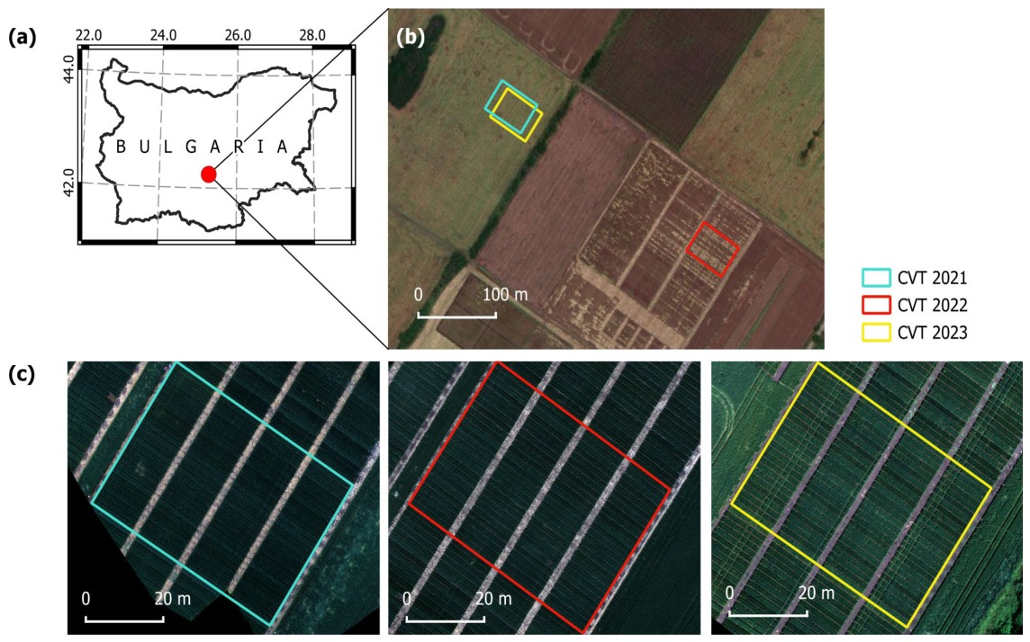
Figure 1. (a) Location of the study area in Bulgaria. (b) Location of the experimental fields for 2021, 2022, and 2023 (Background Image: © 2025 Microsoft Bing Maps, Redmond, WA, USA; © 2025 Maxar, Westminster, CO, USA). (c) Close-up views of the experimental fields showing field outlines and the UAV mosaics generated in this study in the band combination of red, green, and blue.
Remotesensing 18 02664 g001
Figure 2. Overview of data acquisition, processing workflow, and analytical methods for genotype characterization using UAV multispectral data, field traits, and meteorological variables. Abbreviations: GPC—grain protein content; PY—protein yield; LAI—leaf area index; LCC—leaf chlorophyll content; GPR—Gaussian process regression; QRF—quantile regression forest; NDRE—normalized difference red-edge index.
Remotesensing 18 02664 g002
Figure 3. Monthly mean air temperature (a) and precipitation sums (b) for the three growing seasons and for the 1928–2023 multi-year norm. The precipitation sum for the October–July period is also shown in (b).
Remotesensing 18 02664 g003
Table 1. UAV flight missions’ dates, the corresponding phenophases (BBCH code, [41]) of the winter durum wheat genotypes, and the weather conditions during the flights.
Flight Mission IDFlight DateBBCH CodeWeather Conditions
FM127 May 2021BBCH 69 (18 genotypes) and BBCH 71 (8 genotypes)Clear sky
FM226 May 2022BBCH 71 (26 genotypes)Clear sky
FM325 May 2023BBCH 69 (11 genotypes) and BBCH 71 (15 genotypes)Clear sky
Table 2. Descriptive statistics of the ground-measured parameters at the genotype level.
ParameterSeasonDateNumber of MeasurementsMin.Max.MeanStd. Dev.CV %
Yield [kg per plot]/[Mg·ha−1]202115 July1048.32/6.3010.39/7.879.55/7.230.55/0.425.76
202211 July1046.67/5.059.46/7.178.47/6.420.62/0.477.32
202313 July1044.36/3.307.86/5.955.69/4.310.79/0.6013.88
Grain protein content [%]202115 July10413.8515.4814.470.412.83
202211 July10414.2816.4015.450.462.98
202313 July10411.7013.5812.650.463.64
Protein yield [kg protein per plot]202115 July1041.221.501.380.075.07
202211 July1041.041.441.310.118.40
202313 July1040.580.950.720.0912.50
Heading date 12021-1041391471432.571.80
2022-1041391461422.051.45
2023-1041331441393.042.19
Plant height [cm]202127 May10489.7114.5101.95.04.88
202227 May10480.299.187.85.46.11
202326 May10496.1125.8104.06.76.48
Leaf Area Index [m2·m−2]202127–28 May524.46.55.30.59.43
202225–26 May524.06.65.00.816.00
202325–26 May524.88.66.81.217.65
Leaf Chlorophyll Content [mg·m−2]202127–28 May52440.8505.0477.016.73.50
202225–26 May52395.9502.6456.930.66.70
202325–26 May52376.0500.1446.033.97.60
Number of productive tillers202110 July1043540.512.50
20228 July1044540.37.50
202110 July1045650.48.00
1 The days to heading are calculated from 1 January.
Table 3. Spectral and texture features showing significant correlation (p < 0.05) with yield, grain protein content (GPC), and protein yield (PY) in at least two seasons. In each group, the feature with the highest correlation across all seasons is shown in bold.
FeaturesYieldGPCPY
SpectralNDRE, Green, mNDblue, MTCI, CIred-edge-NDRE, Green, Red, GNDVI, mNDblue, MTCI, CIred-edge, CIgreen
TextureMeaGreen3-MeaRed3, MeaGreen3
Table 4. Results of analysis of variance (ANOVA) for the agronomic traits—Yield, Grain Protein Content (GPC), and Protein Yield (PY)—and for the selected UAV features—NDRE, MeaGreen3, and MeaRed3.
Source of VariationSSdfMSSignificantη2 %
Yield
Environment827.822413.91***82.08
Genotype63.69252.55***6.31
E × G67.07501.34***6.65
Error49.902340.21 4.94
GPC
Environment420.072210.03***86.53
Genotype40.44251.62***8.33
E × G19.27500.39***3.96
Error5.672340.02 1.16
PY
Environment27.5469213.7734***88.81
Genotype1.2271250.0491***3.94
ExG1.2161500.0243***3.90
Error1.04642340.0045 3.35
NDRE
Environment0.265120.1325***69.06
Genotype0.0436250.0017***11.37
ExG0.0169500.0003ns4.40
Error0.05832340.0002 15.18
MeaGreen3
Environment40.93220.47***4.72
Genotype488.062519.52***56.34
ExG111.17502.22***12.83
Error225.982340.97 26.09
MeaRed3
Environment74.82237.41***7.73
Genotype339.292513.57***35.07
ExG158.81503.18***16.41
Error394.312341.69 40.76
ns p > 0.05; *** p < 0.001.
Table 5. Performance of regression models predicting agronomic traits from UAV-derived spectral and texture features and explanatory agronomic traits. Cross-validation metrics are presented as value ± standard deviation across folds, while independent validation metrics represent performance on the unseen validation dataset.
ModelCross-Validation Metrics (Value ± SD)Independent Validation MetricsRelevant Features
GPR YieldR2 = 0.76 ± 0.05; RMSE = 0.89 ± 0.04;
nRMSE = 14.76 ± 0.33
R2 = 0.54; RMSE = 1.18;
nRMSE = 22.31
Plant Height, MTCI, NGBDI, DVI, VarBleu3, CorGreen3
GPR GPCR2 = 0.86 ± 0.04; RMSE = 0.45 ± 0.06;
nRMSE = 10.35 ± 2.10
R2 = 0.64; RMSE = 0.78;
nRMSE = 17.85
SR, repRVI, NDVI, SIPI, NGBDI, CIgreen, PSRI, SAVI, DVI, ASMRed3, MeaRed3, VarRE3, CorBlue3, CorGreen3
GPR PYR2= 0.85 ± 0.14; RMSE = 0.12 ± 0.05;
nRMSE = 13.38 ± 5.55
R2 = 0.86, RMSE = 0.12;
nRMSE = 14.02
DVI, CorRE3, CorRed3
QRF YieldR2 = 0.71 ± 0.20; RMSE = 0.97 ± 0.29;
nRMSE = 16.07 ± 4.33
R2 = 0.71; RMSE = 0.95;
nRMSE = 17.91
mNDblue, NGBDI
QRF GPCR2 = 0.76 ± 0.21; RMSE = 0.60 ± 0.22;
nRMSE = 13.88 ± 5.36
R2 = 0.79; RMSE = 0.66;
nRMSE = 15.24
NGBDI, CorBlue3
QRF PYR2 = 0.72 ± 0.28; RMSE = 0.17 ± 0.08;
nRMSE = 18.35 ± 9.37
R2 = 0.76; RMSE = 0.15;
nRMSE = 18.68
Blue, NIR, NDVI, mNDblue, NGBDI, ASMNIR3, EntNIR3
Table 6. Season-specific predictive performance of the best-performing models applied to the complete dataset.
ModelAll Data 2021All Data 2022All Data 2023
GPR YieldR2 = 0.47; RMSE = 0.59;
nRMSE = 28.71
R2 = 0.63; RMSE = 0.59;
nRMSE = 21.08
R2 = 0.45; RMSE = 0.74;
nRMSE = 21.13
GPR GPCR2 = 0.39; RMSE = 0.51;
nRMSE = 31.51
R2 = 0.53; RMSE = 0.34;
nRMSE = 15.79
R2 = 0.29; RMSE = 0.40;
nRMSE = 21.53
GPR PYR2 = 0.58; RMSE = 0.05;
nRMSE = 18.09
R2 = 0.78; RMSE = 0.05;
nRMSE = 12.57
R2 = 0.37; RMSE = 0.08;
nRMSE = 22.24
QRF YieldR2 = 0.24; RMSE = 0.48;
nRMSE = 23.07
R2 = 0.42; RMSE = 0.60;
nRMSE = 21.62
R2 = 0.20; RMSE = 1.14;
nRMSE = 32.71
QRF GPCR2 = 0.21; RMSE = 0.40;
nRMSE = 24.38
R2 = 0.44; RMSE = 0.38;
nRMSE = 17.98
R2 = 0.11; RMSE = 0.66;
nRMSE = 35.25
QRF PYR2 = 0.39; RMSE = 0.05;
nRMSE = 18.97
R2 = 0.54; RMSE = 0.08;
nRMSE = 20.65
R2 = 0.21; RMSE = 0.17;
nRMSE = 47.10
Disclaimer/Publisher’s Note: The statements, opinions and data contained in all publications are solely those of the individual author(s) and contributor(s) and not of MDPI and/or the editor(s). MDPI and/or the editor(s) disclaim responsibility for any injury to people or property resulting from any ideas, methods, instructions or products referred to in the content.