Sensitivity-Constrained Anisotropic Regularization for Two-Track InSAR 3D Landslide Deformation Inversion in the Baihetan Reservoir Area, China

Highlights

What are the main findings?

• A sensitivity-constrained anisotropic regularization framework was developed for 3D landslide deformation inversion from two-track InSAR observations, stabilizing weakly constrained deformation components in complex reservoir-bank terrain.
• The method mapped post-impoundment 3D deformation in the Baihetan Reservoir, revealed localized active landslides with coupled subsidence, horizontal displacement, and downslope creep, and identified rainfall and reservoir-level response lags for the Xiaomidi landslide.

What are the implications of the main findings?

• The proposed framework provides a practical solution for reliable 3D landslide deformation recovery when only two SAR viewing geometries are available, overcoming weak direction instability and the limitations of conventional isotropic regularization in mountainous regions.
• By integrating stable 3D motion decomposition, slope-coordinate interpretation, GNSS validation, field evidence, and hydrological time lag analysis, this study strengthens post-impoundment landslide risk diagnosis and supports more physically interpretable monitoring of reservoir-bank slopes.

Abstract

Interferometric synthetic aperture radar (InSAR) is a key tool for monitoring landslide deformation in reservoir regions. However, when only ascending and descending line-of-sight (LOS) observations are available, 3D deformation inversion over complex hillslopes remains challenging because of slope-geometry priors and the anisotropic observation sensitivity. This study focuses on hillslopes in the Baihetan Reservoir area after impoundment. We use 340 ascending and descending Sentinel-1A images acquired from April 2021 to October 2024, generating LOS displacement time series using the extended small baseline subset (E-SBAS) technique. We propose a two-track InSAR 3D inversion framework centered on sensitivity-constrained anisotropic regularization (SC-Aniso). In this framework, a local-gradient surface-parallel flow model (LGSPFM) serves as a supporting pixel-scale topographic prior for representing local slope geometry. SC-Aniso constitutes the primary methodological innovation by mapping the inverse joint LOS sensitivities of the E, N, and U components to component-wise regularization weights. This design suppresses noise amplification in weakly constrained directions. Results show that the Baihetan Reservoir area is generally stable, with localized anomalies mainly in typical reservoir-bank landslide zones. The inverted 3D fields reveal coupled subsidence, horizontal displacement and downslope creep in the L01–L03 landslides. GNSS validation shows vertical RMSEs below 5.29 mm, mean 3D rate differences below 4 mm/yr, and an average component-wise rate difference of 2.56 mm/yr. At the optimal regularization parameter, SC-Aniso reduces north–south dispersion in stable areas by 41.9% compared with isotropic regularization. Wavelet analysis indicates a 288–384 day seasonal period for nonlinear displacement of the Xiaomidi landslide, with lags of 24 and 90 days relative to precipitation and reservoir water level, respectively. This study provides support for accurately recovering 3D deformation and interpreting movement mechanisms of landslides under limited two-track LOS observations.

1. Introduction

In deep canyon reservoir areas, hillslope instability is not only controlled by lithology, geological structure and topography, but also by the combined effects of cyclic reservoir-level fluctuations and rainfall [1,2,3]. Such hillslope deformation is commonly slow, hidden and spatially heterogeneous. Therefore, a limited number of ground-based monitoring points cannot fully characterize its regional distribution [4,5]. Time-series InSAR can provide millimetre-scale measurements of surface deformation over large areas, and persistent scatterer (PS) and small baseline subset (SBAS) approaches have been widely used for monitoring ground deformation and hillslope activity [6,7]. However, single-track InSAR observations only provide projected displacement in the radar line-of-sight (LOS) direction [8,9]. When hillslope movement includes both horizontal and vertical components, LOS deformation is difficult to directly reflect the true direction of movement [10,11]. Using multi-track or multi-view observations to recover three-dimensional deformation has become an important direction for improving the kinematic interpretation of landslides [12,13].

Currently, multi-track InSAR fusion, 2D deformation visualization, and surface-parallel flow models have been used to interpret unstable hillslope motion [12,14,15,16,17,18]. In the absence of a third independent observation component, the surface-parallel flow model (SPFM) utilizes the physical constraint that hillslope motion is approximately parallel to the slope surface to transform dual-track LOS data into 3D landslide deformation estimation, and has been applied in various landslide scenarios [14,15,16,19,20,21]. Recent studies have further introduced pixel-scale slope and aspect, local parallel flow, or pixel-level surface-parallel flow constraints into landslide motion identification to reduce the overgeneralization of overall average slope parameters for complex terrain [19,20]. These studies indicate that local slope geometric constraints have become an important direction for 3D landslide inversion using dual-track InSAR, but the stability calculation of weakly sensitive directions and the problem of observation geometric imbalance remain unresolved challenges.

Despite these advances, 3D deformation inversion under dual-track InSAR conditions still faces two key limitations. First, the overall average slope and average aspect in traditional SPFM are insufficient to characterize the fragmented terrain and rapidly changing aspect of canyon hillslopes [15,19,20]. Pixel-scale or local slope constraints can improve this averaging problem [19,20], but their primary function remains providing topographical priors. Second, ascending and descending Sentinel-1 LOS observations have uneven sensitivity to different deformation components, with particularly weak constraints on the north–south component. Direct inversion or isotropic regularization can easily lead to amplification of noise in the weakly sensitive directions [10,11,22,23,24]. Therefore, based on existing local slope geometric priors, further constructing a directional stabilization strategy that conforms to the observed geometric characteristics is crucial for improving the reliability of 3D InSAR inversion of reservoir bank landslides.

The Baihetan Hydropower Station is an important component of the giant cascade hydropower project on the lower reaches of the Jinsha River. The reservoir area has steep hillslopes, deep valleys, and complex geological lithology [25,26]. After initial impounding in 2021, the reservoir entered a stage of high-water-level operation and periodic scheduling [27,28,29]. Existing studies have shown that large ancient landslides, bank collapses, and potentially unstable slopes are widely developed in the Baihetan Reservoir area and the adjacent Jinsha River section [25,26,28]. Their spatial distribution is jointly controlled by factors such as valley cutting, fault structures, slope and aspect, and reservoir water level changes [25,27,28]. However, existing studies focus more on landslide identification, spatial distribution, or single LOS deformation characteristics. Comprehensive research on the three-dimensional motion field after impoundment, weakly sensitive directional stability inversion, and landslide hydrological response mechanisms is still relatively insufficient.

To solve the above problems, we focus on post-impoundment reservoir hillslopes in the Baihetan Reservoir area and construct a 3D deformation inversion and mechanism interpretation framework for dual-track InSAR. We use 340 ascending and descending track Sentinel-1A scenes to derive LOS time-series deformation over the reservoir area from 2021 to 2024. Building on existing SPFM and pixel-scale surface-constraint concepts, we introduce a local-gradient surface-parallel flow model (LGSPFM) constraint as a topographic prior in the dual-track inversion, thereby representing pixel-scale surface geometry. We propose the sensitivity-constrained anisotropic regularization (SC-Aniso) strategy to adaptively stabilize the three-dimensional component solution based on the inverse relationship of the observed geometric sensitivity. The accuracy of the method is evaluated by combining GNSS monitoring data. The deformation mechanism of landslides is explained by field investigation and rainfall-reservoir water level time–frequency analysis. Within the proposed framework, LGSPFM provides a supporting pixel-scale topographic prior based on existing SPFM concepts, while SC-Aniso represents the primary methodological advance of this study. SC-Aniso explicitly incorporates the directional sensitivity imbalance of dual-track LOS observations into the regularization design. Its effectiveness is quantitatively evaluated through synthetic experiments, GNSS validation, and a stability–fitting trade-off analysis.

2. Study Area

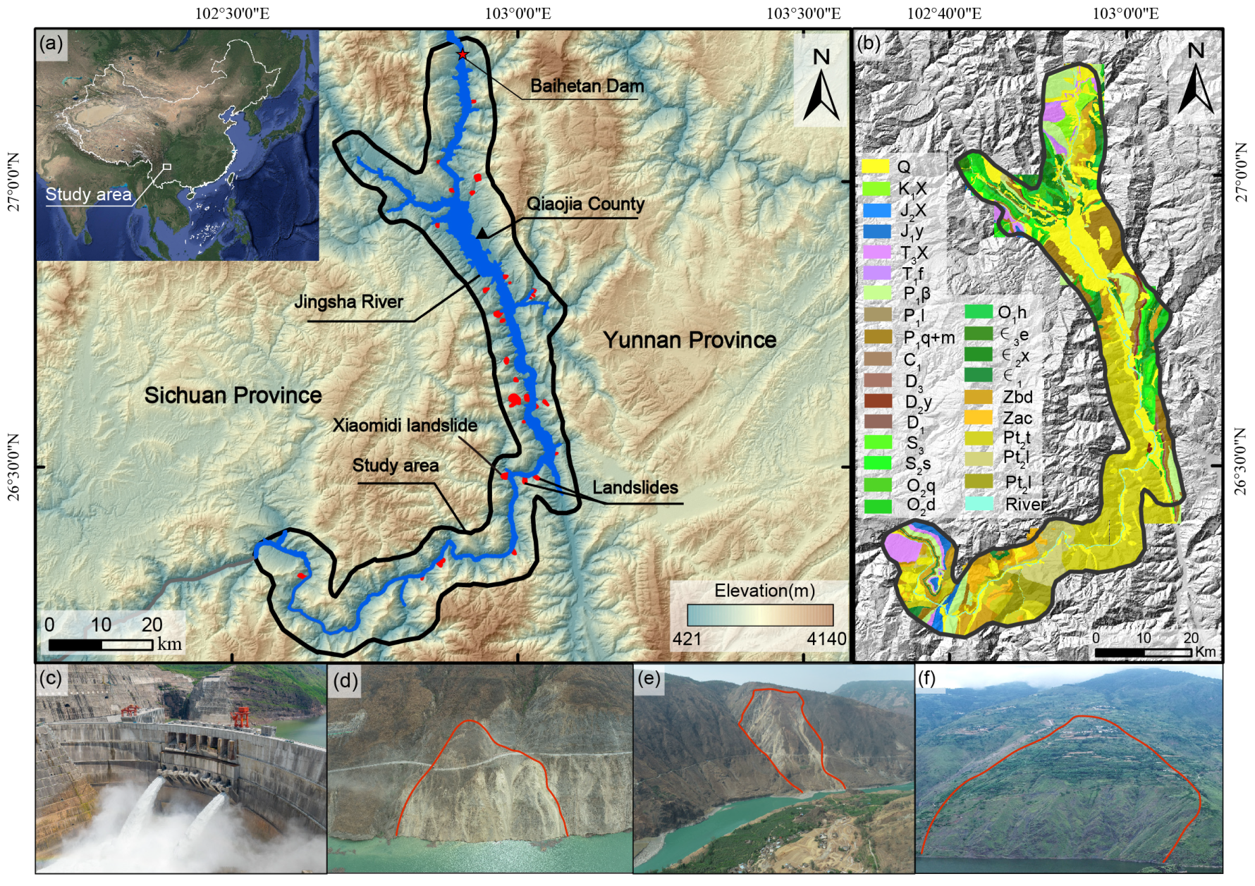
The Baihetan reservoir area is located in the transition zone between the southeastern edge of the Qinghai–Tibet Plateau and the northeastern part of the Hengduan Mountains. The terrain is characterized by large elevation differences, steep slopes, and deep valleys, with intense regional tectonic activity [25,26,29]. The dam site spans Ningnan County in Sichuan Province and Qiaojia County in Yunnan Province (Figure 1a), approximately 182 km upstream from the Wudongde Hydropower Station and approximately 195 km downstream from the Xiluodu Hydropower Station. The study area is approximately 1779.88 km². The Baihetan Reservoir began impounding water on April 6, 2021, and reached its normal impoundment level of 825 m for the first time in late October 2022 [28]. Since then, the reservoir has entered the stage of routine regulation, with the water level fluctuating periodically mainly between approximately 770 and 825 m [28].

The study area is located in the hinterland of southwest China, belonging to the subtropical climate zone. The highest temperature throughout the year is 42.7 °C, the lowest temperature is −0.4 °C, and the average annual temperature is 7.1–21.1 °C [26,28]. Precipitation is strongly seasonal, with rainfall concentrated mainly from May to October each year [26,28]. The study area is situated in the transition zone between the first and second steps of China’s terrain, characterized by complex geological conditions, diverse stratigraphic combinations, and stratigraphic ages ranging from the Precambrian to the Quaternary (Figure 1b). Intense tectonic activity, complex lithology, steep terrain, concentrated seasonal rainfall, and reservoir water level fluctuations all contribute to the high sensitivity of the study area to landslides [25,27,30]. Especially after impoundment, the periodic rise and fall of the reservoir water level significantly altered the hydrogeological conditions of the reservoir hillslopes, providing important external factors for hillslope deformation and landslide development, resulting in numerous deformed hillslopes in the study area (Figure 1d–f) [28,31].

3. Materials and Methods

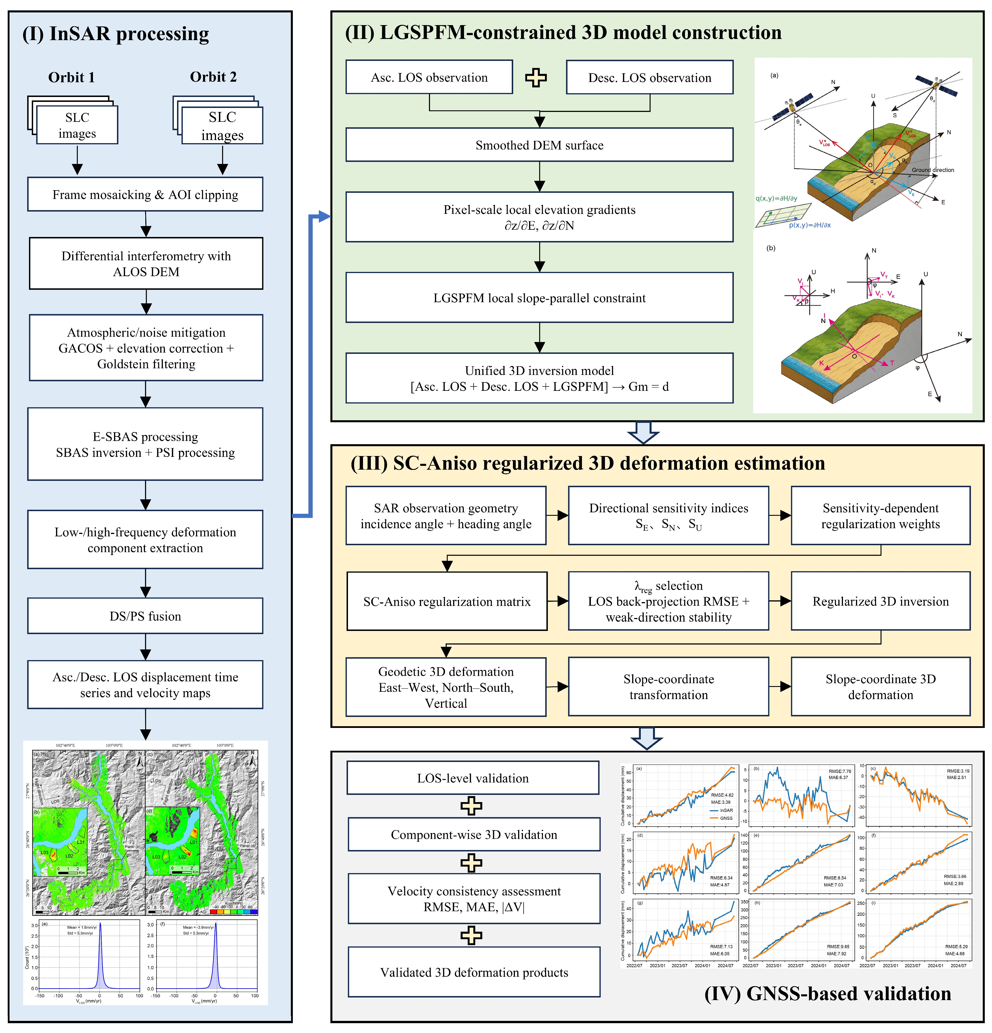
Our methodology consists of four key steps: (i) generating the time-series LOS deformation of the Baihetan Reservoir area after impoundment using ascending and descending orbit Sentinel-1A data; (ii) integrating ascending and descending LOS observations with pixel-scale local elevation gradients derived from the DEM, and introducing a local surface-parallel-flow topographic constraint to establish a three-dimensional deformation inversion model; (iii) constructing the SC-Aniso anisotropic regularization matrix based on the observation sensitivity in different directions, and estimating the 3D deformation components in both the geodetic and slope-coordinate systems; and (iv) validating the inverted 3D deformation using in situ GNSS measurements. The detailed technical workflow is shown in Figure 2.

3.1. Materials

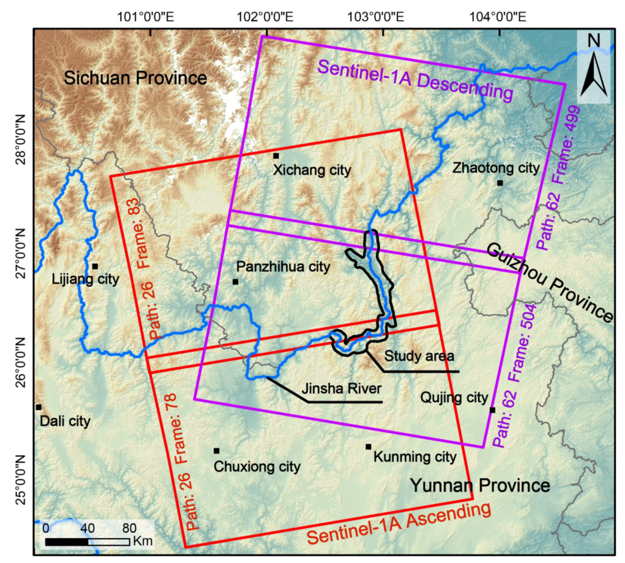
In this study, we collected 340 SAR images, including Sentinel-1A ascending and descending orbit datasets, to reconstruct the historical displacement of the Baihetan Reservoir area over the four years after impoundment, spanning from April 2021 to October 2024. Owing to its particular geographic setting, the study area is located within the overlap zone of two adjacent Sentinel-1A tracks acquired in interferometric wide-swath mode (Figure 3). Sentinel-1 is an Earth observation mission of the European Space Agency (ESA), consisting of two satellites launched in 2014 and 2016. The images have a spatial resolution of approximately 5 m × 20 m and a revisit interval of 12 days [32]. In this study, VV polarization data were used, and detailed information is provided in

Table 1. Specific information on SAR data for the study area.

Satellite	Path	Frame	Polarization	Beam	Orbit	Heading (°)	Incidence Angle (°)	Acquisition Dates (dd/mm/yyyy)	Total Image Number
Sentinel-1A	62	499 (83 images) and 504 (83 images)	VV	IW	Descending	192.5	38.9	11 April 2021–10 April 2024	166
Sentinel-1A	26	78 (87 images) and 83 (87 images)	VV	IW	Ascending	342.5	40.9	9 April 2021–2 October 2024	174

. Sentinel-1 SAR images have been widely applied to ground deformation and landslide monitoring [33]. Notably, the ascending- and descending-track Sentinel-1A datasets have overlapping or closely spaced acquisition dates, which makes 3D deformation inversion in the study area possible.

We also collected precise orbit data time-consistent with the SAR data for orbit correction. In addition, we selected ALOS 12.5 m DEM data [34] as the digital elevation model (DEM) to eliminate terrain errors. To mitigate atmospheric delay errors after reservoir impoundment, we acquired GACOS data (http://www.gacos.net, accessed on 28 March 2026) [35] that was time-consistent with the SAR data. Finally, to verify the accuracy of InSAR 3D deformation, we obtained GNSS measurement data from the Xiaomidi landslide site for verification.

3.2. Methods

3.2.1. InSAR Processing for LOS Deformation

LOS deformation is the basis for inverting three-dimensional deformation. To generate LOS surface deformation over the study area, we used the enhanced SBAS (E-SBAS) method implemented in SARscape 5.7 [7,36,37,38,39]. This method integrates distributed scatterer (DS) and persistent scatterer (PS) information [6,37,39] within the conventional SBAS time-series analysis framework [7,38], allowing more reliable measurement points to be retained in both vegetated mountainous areas and exposed artificial-target areas. DS and PS are used to improve spatial coverage and local precision, respectively. DS information is mainly obtained from SBAS interferograms processed with multi-looking and spatial filtering. It is used to derive a relatively continuous low-frequency deformation field. PS information is extracted from interferograms without strong spatial filtering. Highly coherent and temporally stable scatterers are identified to supplement local high-frequency deformation information. The DS and PS deformation results are then unified using the same reference point, temporal datum, and geographic coordinate system. Finally, they are merged to generate the LOS displacement time series and mean deformation velocity dataset.

Because the study area is covered by two SAR scenes acquired along the same track (Figure 3), the SAR images were first mosaicked and then clipped to the boundary of the study area, following the preprocessing strategy of Cigna and Tapete [36]. To reduce the influence of temporal decorrelation on interferometric quality [40], the temporal baseline threshold was set to 60 days during interferometric pair generation, and valid interferograms were selected by considering spatial baseline and coherence conditions.

The E-SBAS processing consisted of two main stages: standard SBAS inversion and extraction of high-frequency deformation information from highly coherent targets. First, differential interferograms were generated, followed by adaptive Goldstein filtering [41], phase unwrapping and time-series inversion. The topographic phase was estimated and removed using the ALOS DEM, and precise orbit data were used to reduce orbital errors. To mitigate tropospheric delay effects, we applied external atmospheric correction using GACOS products and further reduced residual atmospheric phase using a linear elevation-dependent model [35,42]. The multi-looking factors in the azimuth and range directions were set to 2:8, respectively, and the ratio between the minimum and maximum Goldstein filtering parameters was set to 1:4. These procedures were designed to reduce the influence of noise on the deformation estimates.

After atmospheric correction and residual topographic error removal, the low-frequency components of the deformation field and topographic error were first extracted from the SBAS results. Subsequently, the PSI concept was introduced using interferograms without strong spatial filtering to identify stable PS targets and extract their high-frequency deformation information [6,37,39]. By combining the low-frequency SBAS results with the high-frequency PSI results, DS and PS targets were jointly modelled, thereby balancing spatial coverage with the deformation accuracy of locally coherent targets.

Finally, the time-series displacement results of the two types of scatterers were integrated into a unified dataset, from which ascending- and descending-track LOS displacement time series and mean deformation velocities were obtained for the study area. Compared with the conventional SBAS method, E-SBAS can retain more valid observations in areas with relatively low coherence, such as vegetated and mountainous terrain, and can more comprehensively characterize the spatial distribution of complex surface deformation.

3.2.2. 3D Deformation Field Modeling Using Two-Track Observations and LGSPFM

InSAR observations essentially record the projection of 3D surface deformation onto the radar line-of-sight (LOS) [8,42]. In this study, 3D deformation is represented by the eastward, northward and vertical components in the geodetic coordinate system, where the positive directions of E, N and U are defined as eastward, northward and upward, respectively [10,42]. A negative U value indicates subsidence. The projection relationship between the LOS velocity $V_{LOS}$ and the 3D deformation components [10,42] can be expressed as:

$$V_{LOS}=-\mathrm{s}\mathrm{i}\mathrm{n}\theta \cdot \mathrm{s}\mathrm{i}\mathrm{n}\left(\alpha -{\displaystyle \frac{3\pi }{2}}\right)\cdot V_E-\mathrm{s}\mathrm{i}\mathrm{n}\theta \cdot \mathrm{c}\mathrm{o}\mathrm{s}\left(\alpha -{\displaystyle \frac{3\pi }{2}}\right)\cdot V_N+\mathrm{c}\mathrm{o}\mathrm{s}\theta \cdot V_U$$

(1)

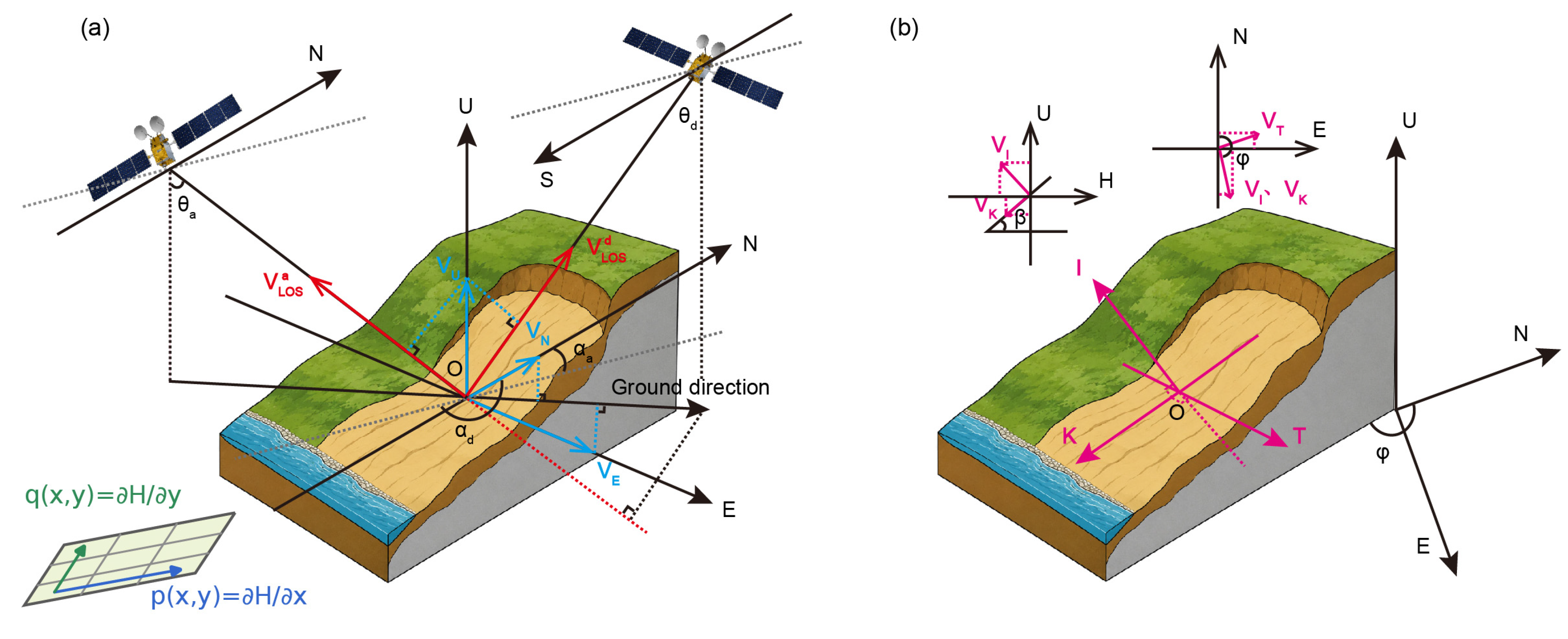
where $V_{LOS}$ is the LOS deformation velocity; $V_E$, $V_N$, and $V_U$ are the eastward, northward, and vertical deformation-velocity components, respectively; $\theta$ is the radar incidence angle; and $\alpha$ is the satellite heading angle. Equation (1) contains three unknown deformation components, whereas a single-track LOS observation provides only one-dimensional projected displacement information, making it difficult to independently recover the full 3D deformation field. In theory, at least three mutually independent observation components with sufficiently distinct viewing geometries are required to invert the complete 3D deformation field without prior constraints [10,11,12]. However, the study area lacks sufficient orbital coverage to satisfy this requirement. To overcome this limitation, we jointly used ascending- and descending-track LOS surface deformation observations, together with the LGSPFM constraint, to solve for the 3D surface deformation. Figure 4 illustrates the schematic principle of 3D deformation inversion based on ascending and descending track LOS observations. Before the 3D inversion, the ascending and descending track LOS datasets were spatially matched. Only locations with valid measurements in both datasets were retained as common valid measurement points.

We improved the SPFM topographic constraint originally proposed by Joughin et al. [14]. The surface-parallel flow model (SPFM) generally assumes that hillslope movement is parallel to the ground surface and uses the mean slope and mean aspect to describe the terrain geometry. This assumption is particularly suitable for gravity-driven hillslope movements, such as landslides, snow avalanches and rock glaciers [14,15,16]. However, in areas with complex topographic relief and pronounced local variations in hillslope morphology, spatially averaged slope parameters often cannot accurately represent the local geometric characteristics at the pixel scale [19,20]. Therefore, we adopted the LGSPFM to improve the conventional SPFM. Instead of using mean slope or mean aspect, the proposed approach calculates the local elevation gradient at the pixel scale from a smoothed DEM and replaces the globally averaged slope surface with a local tangent-plane approximation. In this way, the surface-parallel constraint can respond more precisely to the spatial heterogeneity of the terrain. To better characterize the local geometric properties of complex hillslopes at the pixel scale, the original DEM was first smoothed to obtain a locally smoothed topographic surface:

$$\tilde{H}\left(x,y\right)={\displaystyle \frac{\sum _{(u,vϵN_r(x,y\left)\right)}{\omega }_{uv}\cdot H(u,v)}{\sum _{(u,vϵN_r(x,y\left)\right)}{\omega }_{uv}}}$$

(2)

where $H\left(u,v\right)$ denotes the elevation value of the original DEM, and ${\omega }_{uv}$ is the distance-weighted coefficient of the pixels within the local neighbourhood. In this study, Gaussian low-pass smoothing was applied to reduce the influence of microtopographic noise on the estimation of local surface geometry. We tested multiple Gaussian smoothing scales with standard deviations ranging from 0.1 to 5.0 pixels. We truncated the Gaussian kernel radius at 4σ. We ultimately adopted σ = 1.0 pixel, corresponding to a 9 × 9-pixel Gaussian kernel. This setting provided a conservative balance between reducing local-gradient roughness and limiting changes to the original DEM. Based on the smoothed DEM, the first-order gradients of the local terrain in the east–west and north–south directions were calculated as follows:

$$p\left(x,y\right)={\displaystyle \frac{\partial \tilde{H}}{\partial x}},q\left(x,y\right)={\displaystyle \frac{\partial \tilde{H}}{\partial y}}$$

(3)

where $p(x,y)$ and $q(x,y)$ denote the pixel-scale local elevation gradients of the slope surface in the east–west and north–south directions, respectively. Under the LGSPFM assumption, the 3D deformation vector in the geodetic coordinate system, $V={{[V}_E,V_N,V_U]}^T$ satisfies the following local surface constraint:

$$V_U=p\left(x,y\right)V_E+q\left(x,y\right)V_N$$

(4)

where $V_E,V_N$ and $V_U$ denote the eastward, northward and vertical deformation components, respectively. By combining Equations (1) and (4), the dual-track LOS observations and the LGSPFM topographic constraint can be written in a unified 3D deformation model in the geodetic coordinate system:

$$V_{obs}=G\cdot m$$

(5)

$$V_{obs}=\left[\begin{array}{c}{V}_{LOS}^a\\ V_{LOS}^d\\ 0\end{array}\right]$$

(6)

$$G=\left[\begin{array}{ccc}-sin{\theta }_{a}sin({\alpha }_a-3\pi /2)& -sin{\theta }_{a}cos({\alpha }_a-3\pi /2)& cos{\theta }_a\\ -sin{\theta }_{d}sin({\alpha }_d-3\pi /2)& -sin{\theta }_{d}cos({\alpha }_d-3\pi /2)& cos{\theta }_d\\ -p& -q& 1\end{array}\right]$$

(7)

In Equation (5), $V_{obs}$ denotes the observation vector, $G$ is the design matrix describing the relationship between the dual-track observations, the LGSPFM topographic constraint and the 3D deformation components, and $m$ is the unknown parameter vector to be estimated, defined as $m={[V_E,V_N,V_U]}^T$. In Equation (6), the superscripts (a) and (d) denote the parameters and LOS observations of the ascending and descending tracks, respectively.

After obtaining the 3D deformation in the geodetic coordinate system, we further transformed the results into the slope coordinate system to better characterize the kinematic features of landslide or slope deformation under local slope conditions. This transformation yields the downslope component $V_K$, the cross-slope component $V_T$ and the normal-to-slope component $V_I$. Let the local slope angle and aspect be denoted by $\beta$ and $\phi$, respectively. The coordinate transformation between the geodetic coordinate system and the slope coordinate system can then be expressed as follows:

$$\left[\begin{array}{c}{V}_K\\ V_T\\ V_I\end{array}\right]=\left[\begin{array}{ccc}-cos\beta sin\phi & -\mathit{cos}\beta cos\phi & sin\beta \\ -cos\phi & sin\phi & 0\\ sin\beta sin\phi & sin\beta cos\phi & cos\beta \end{array}\right]\left[\begin{array}{c}{V}_E\\ V_N\\ V_U\end{array}\right]$$

(8)

3.2.3. 3D Deformation Estimation Based on Sensitivity-Constrained Anisotropic Regularization

Although Equation (5) integrates the dual-track LOS observations and the LGSPFM topographic constraint into a unified 3D deformation model, the observability of deformation components in different directions remains uneven because of the limitations imposed by the ascending and descending SAR imaging geometries [10,11,12,22,23]. In particular, the north–south component usually has weak sensitivity to LOS observations and is therefore more susceptible to noise amplification and error propagation during direct inversion [10,11,22,23]. Conventional isotropic Tikhonov regularization [24,43] applies the same constraint strength to all deformation components, and therefore cannot reflect the differences in the sensitivity of the actual observation geometry to different directional components. This is not conducive to the stable recovery of 3D deformation. To address this issue, we constructed a sensitivity-constrained anisotropic regularization (SC-Aniso) strategy, in which the regularization strength is adaptively adjusted according to the observation sensitivity in different directions.

To quantitatively describe the constraining capability of the observation geometry for different directional components, the LOS observation can be expressed as $V_{LOS}=r^T\cdot m$, where $r={[r_E,r_N,r_U]}^T$ is the LOS unit vector. The directional sensitivity of the (i)-th deformation component can then be defined as the absolute value of the first-order partial derivative of the LOS observation with respect to that component. The sensitivities in different directions are calculated as follows:

$$S_E=\left|-\cos \alpha \cdot \sin \theta \right|$$

(9)

$$S_N=|\sin \alpha \cdot \sin \theta |$$

(10)

$$S_U=\left|\cos \theta \right|$$

(11)

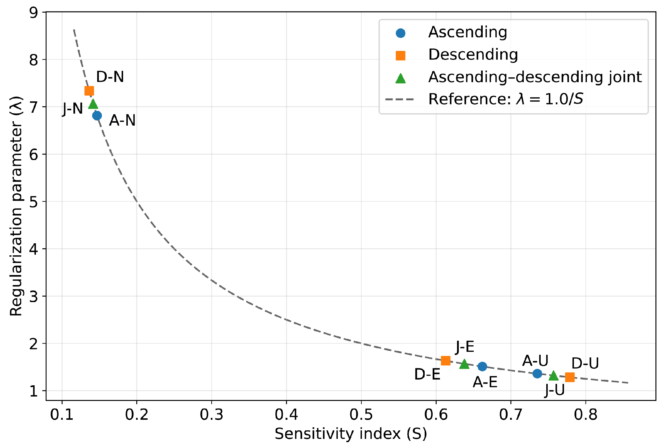
In the above equations, $S_E$, $S_N$ and $S_U$ denote the sensitivities to east–west, north–south and vertical deformation, respectively. $\theta$ represents the incidence angle, and $\alpha$ denotes the heading angle. For the joint ascending and descending track observations, we used the root-mean-square value of the ascending- and descending-track sensitivities to characterize the average observational capability in each direction. The directional regularization parameters, ${\lambda }_i$ ($i \in E, N, U$) were defined according to the inverse relationship with the mean sensitivity in each direction (Figure 5). The resulting regularization-strength ratio among the different directions was set as ${\lambda }_E:{\lambda }_N:{\lambda }_U=1.6:7.1:1.3$. The anisotropic regularization matrix was constructed as follows:

$$W=diag({\mathsf{\lambda }}_E,{\mathsf{\lambda }}_N,{\mathsf{\lambda }}_U)$$

(12)

On this basis, the 3D deformation inversion can be formulated as follows:

$$\widehat{m}=\arg \underset{m}{min} ({\left|\left|G\cdot m-V_{obs}\right|\right|}_2^2+{\mathsf{\lambda }}_{reg}^2\cdot m^T\cdot W\cdot m)$$

(13)

where ${\mathsf{\lambda }}_{reg}$ is the global regularization parameter, which controls the overall balance between the observation-fitting term and the regularization term. $\widehat{m}={[\widehat{V_E},\widehat{V_N,}\widehat{V_U}]}^T$ denotes the estimated 3D deformation components in the geodetic coordinate system obtained using the anisotropic regularization strategy. By differentiating Equation (13) and setting the derivative to zero, the closed-form solution of the 3D deformation can be obtained as follows:

$$\widehat{m}={(G^T\cdot G+{\mathsf{\lambda }}_{reg}^2\cdot W)}^{-1}\cdot G^T\cdot V_{obs}$$

(14)

Mathematically, SC-Aniso is a component-wise, zero-order generalized Tikhonov regularization method. Its anisotropy lies in applying different constraint strengths to the E, N, and U deformation components, rather than in using spatial directional-derivative operators. This differs from weighted least squares. In weighted least squares, weights are applied to the LOS observation residuals to represent differences in error variance or uncertainty among observations [44,45]. In SC-Aniso, the weights are applied in model space through the regularization term to address unequal observability among the deformation components.

Generic weighted or anisotropic Tikhonov regularization allows different penalty strengths to be assigned to different model components or spatial directions [46,47]. Sensitivity-weighted regularization further derives these penalties from the sensitivity of the forward model [47,48]. SC-Aniso belongs to this broad methodological family but adopts an inverse-sensitivity weighting rule tailored to dual-track InSAR.

The relative penalty weight for each of the E, N, and U components is determined by the reciprocal of the corresponding joint root-mean-square sensitivity derived from the actual ascending and descending track LOS geometries. Consequently, more weakly observed deformation components receive stronger damping. Unlike direct sensitivity-weighting schemes [48], which are mainly designed to compensate for sensitivity variations, the inverse-sensitivity weighting used here is intended to suppress noise amplification in weakly observed deformation components. The three directional weights do not need to be tuned independently because their relative proportions are directly determined by the observation geometry. Thus, only a single global regularization parameter ${\mathsf{\lambda }}_{reg}$ needs to be selected during the inversion.

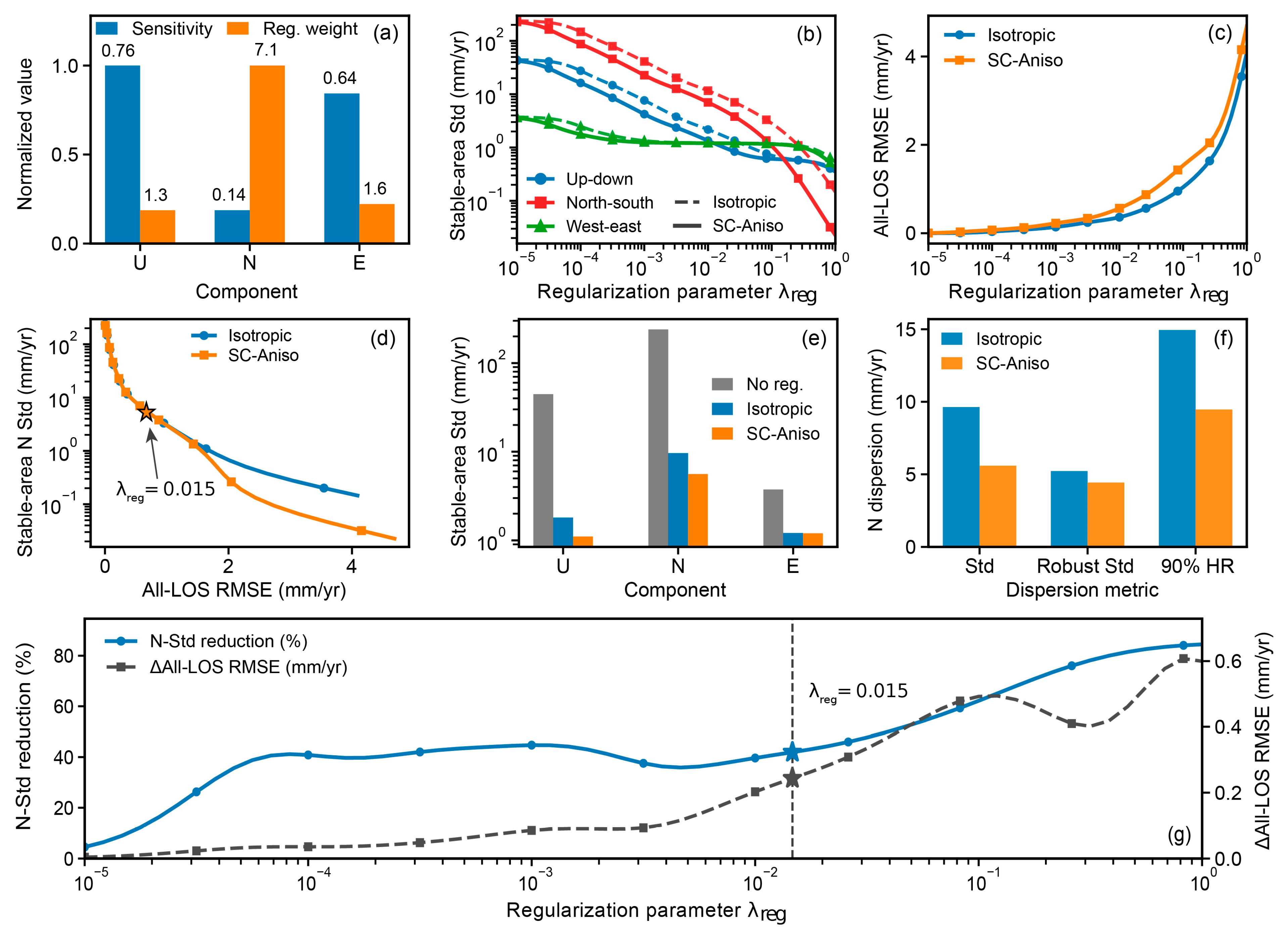
To determine the global regularization parameter objectively, ${\mathsf{\lambda }}_{reg}$ was scanned over a predefined logarithmic grid. The candidate set consisted of 61 logarithmically spaced values from 10⁻⁵ to 10⁰, supplemented by two additional values of 0.015 and 0.02, giving 63 candidate values in total. For each candidate value, we calculated the All-LOS back-projection RMSE and the standard deviation of the north–south component in stable areas. The two metrics were log-transformed and independently normalized to the range of 0–1 to remove scale effects. The objective Pareto knee [49] was defined as the candidate with the maximum perpendicular distance to the chord connecting the two endpoints of the normalized curve. This criterion yielded ${\mathsf{\lambda }}_{reg}$ = 0.015. Section 5.1.2 of the discussion shows the corresponding stability–fitting relationship in the original physical units.

3.2.4. 3D Deformation Accuracy Assessment

To validate the reliability of the inverted 3D deformation, we obtained GNSS monitoring data from the surface of the Xiaomidi landslide in the Baihetan reservoir area and conducted a multi-level accuracy assessment against the InSAR results. This assessment included LOS-direction deformation validation, 3D component-wise deformation validation, and deformation-velocity consistency validation.

For the LOS-direction validation, the east, north and vertical displacement components measured by GNSS were projected onto the satellite line-of-sight direction according to the SAR observation geometry, and then compared with the corresponding InSAR LOS cumulative deformation time series. For the 3D deformation validation, the eastward, northward and vertical cumulative deformation time series inverted from InSAR were compared component by component with the corresponding GNSS displacement series, so as to evaluate the reliability of the 3D decomposition results in different directions. The above accuracy assessments were performed using the mean absolute error (MAE) and root mean square error (RMSE) as evaluation metrics:

$$MAE={\displaystyle \frac{1}{n}}{\displaystyle \sum _{i=1}^n}|X_i^{InSAR}-X_i^{GNSS}|$$

(15)

$$RMSE=\sqrt{{\displaystyle \frac{1}{n}}{\displaystyle \sum _{i=1}^n}{(X_i^{InSAR}-X_i^{GNSS})}^2}$$

(16)

In the above equations, $X_i^{InSAR}$ and $X_i^{GNSS}$ denote the corresponding deformation values from InSAR and GNSS at the (i)-th common observation epoch, respectively. In the LOS validation, $X_i$ represents the cumulative displacement in the LOS direction. In the 3D validation, $X_i$ represents the cumulative displacement in the eastward, northward or vertical direction, respectively. (n) is the number of common valid observation epochs.

To evaluate the consistency of long-term trends, we used the absolute difference between the mean deformation velocities derived from InSAR and GNSS as the evaluation metric, which is expressed as:

$$∆V=|V^{InSAR}-V^{GNSS}|$$

(17)

where $V^{InSAR}$ and $V^{GNSS}$ denote the mean deformation velocities obtained by linear fitting of the InSAR and GNSS time series, respectively. A smaller $∆V$ indicates higher consistency between the InSAR and GNSS results in terms of the long-term deformation trend.

4. Results

4.1. LOS Deformation Velocity Field

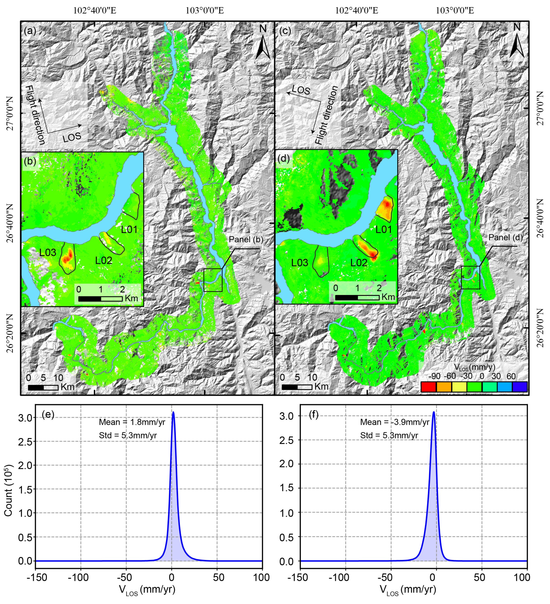
Figure 6 shows the post-impoundment mean LOS deformation velocity fields derived from the ascending and descending tracks, together with enlarged views of the selected landslide areas. Overall, the LOS deformation velocities at most effective InSAR measurement points in the study area are close to a stable state. The frequency distributions of both ascending and descending track velocities exhibit a peak-like distribution centered around 0 mm/yr, indicating good stability of the InSAR processing results at the regional scale. Statistical results show that the mean LOS deformation velocity for ascending tracks is 1.8 mm/yr, with a standard deviation of 5.3 mm/yr; the mean LOS deformation rate for descending tracks is −3.9 mm/yr, also with a standard deviation of 5.3 mm/yr. The relatively small mean values of both tracks indicate that the overall background deformation in the study area is weak, while localized anomalous deformation is mainly concentrated on the reservoir bank slopes and in typical landslide development areas.

Spatially, both the ascending and descending track LOS deformation velocity fields can identify local deformation anomaly zones along the Jinsha River reservoir bank. These anomaly zones are mostly located on bank slopes with significant topographic relief, steep slopes, and proximity to the reservoir water boundary. Compared to the large-scale stable background, L01, L02, and L03 within the typical landslide areas shown in Figure 6b,d all exhibit significant LOS deformation anomalies, indicating that some reservoir bank landslides or potentially unstable slopes remain in a state of continuous activity after impoundment. Although multiple landslides and potentially unstable slopes are distributed in the study area, we primarily selected L01–L03 as test cases based on the InSAR data suitability. All three regions exhibit significant LOS deformation anomalies in both ascending and descending orbit results and possess sufficient common valid measurement points to meet the requirements of subsequent two-orbit 3D deformation inversion. Furthermore, their close spatial proximity provides relatively similar SAR observation geometry, which facilitates the evaluation of the inversion method under comparable observation conditions. Therefore, L01–L03 are mainly used as test cases for method evaluation, rather than representing all landslide types in the Baihetan Reservoir area.

The velocity signs and magnitudes of the same landslide or local deformation zone are not completely consistent between the ascending and descending track LOS results [22,23]. This does not imply a contradiction between the two datasets; rather, it results from differences in the SAR viewing geometries of the ascending and descending tracks. InSAR observations record the projection of 3D ground motion onto the satellite LOS direction. When hillslope movement contains east–west, north–south and vertical components simultaneously, different tracks have different sensitivities to each directional component [10,12,22]. As a result, the same real deformation can exhibit different projected characteristics in the ascending and descending LOS measurements. This effect is particularly evident in complex canyon mountainous areas, where the geometric relationships among the main sliding direction, slope aspect and radar line of sight vary substantially [22,23,26]. Therefore, a single LOS deformation result cannot directly represent the true movement direction of hillslopes.

4.2. 3D Deformation Velocity Field

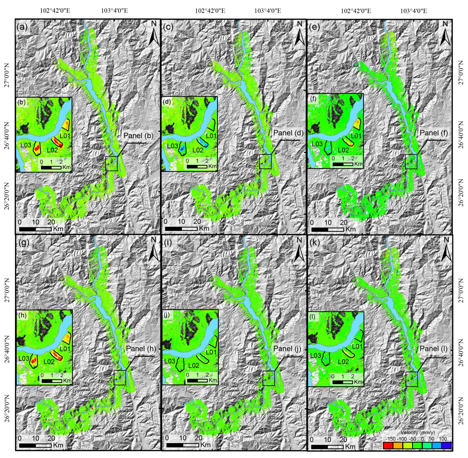
Based on the LOS deformation observation results from the ascending and descending tracks, combined with LGSPFM topographic constraints and the SC-Aniso regularization method, we inverted and obtained the 3D deformation velocity field of the Baihetan Reservoir area after impoundment. Figure 7a–f show the vertical, north–south, and east–west components in the geodetic coordinate system. Positive values indicate upward, northward, and eastward motion, respectively, whereas negative values indicate the opposite directions. Figure 7g–l show the downslope-direction, normal-to-slope, and cross-slope components in the slope-coordinate system. Negative values indicate downslope motion, inward motion toward the local slope surface, and right-lateral motion relative to the local downslope direction, respectively, whereas positive values indicate the opposite directions. Compared with the single LOS results, the 3D deformation results can further reveal the motion components of the reservoir bank landslide in different directions, providing more complete kinematic information for identifying slope deformation patterns.

From the perspective of the 3D deformation components in the geodetic coordinate system, most areas of the study area show relative stability in the vertical, north–south, and east–west directions, with significant anomalies only appearing in local reservoir bank slope areas. Figure 7a,b show that the vertical deformation anomalies are mainly concentrated within and adjacent to the boundaries of typical landslides. Landslides L01–L03 exhibit obvious settlement characteristics, reflecting differential settlement and local unloading processes within the landslide body. Figure 7c,d show that the spatial variation in the north–south deformation component is relatively weak, but certain directional movements can still be identified in the local active areas of typical landslides L02 and L03. Since the Sentinel-1 ascending and descending track LOS observations are generally less sensitive to the north–south component, and the north–south results are more susceptible to noise amplification, the stable recovery of this component also reflects the necessity of sensitivity-constraint regularization. Figure 7e,f show that the east–west deformation component is quite obvious in L01–L03 landslide areas, indicating that there is a significant horizontal movement component in the landslide movement in the study area.

To better interpret the characteristics of hillslope movement, we transformed the 3D deformation components from the geodetic coordinate system into the slope coordinate system. Figure 7g,h show that the downslope deformation velocity more directly highlights the movement of landslides along the slope direction. Compared with the individual vertical, east–west, and north–south components, the downslope component shows a more concentrated response for representative landslides such as L01, L02 and L03, and therefore better reflects the dominant downslope movement tendency of the landslide bodies. Figure 7i,j show that the normal-to-slope deformation mainly represents uplift or subsidence relative to the local slope surface and can be used to identify local compression within landslides. Figure 7j indicates that landslides L01–L03 show relatively weak deformation in this direction. Figure 7k,l show that the cross-slope component reflects lateral differential movement along the slope surface and is useful for identifying secondary deformation units and local lateral shearing within landslides. No obvious deformation signal is observed for landslide L01 in this direction, whereas weak localized deformation signals are present in landslides L02 and L03.

The representative landslides L01, L02 and L03 all exhibit multi-directional compound deformation characteristics, indicating that post-impoundment deformation of reservoir-bank slopes is not a simple process of vertical subsidence or horizontal displacement alone. Instead, it is a 3D movement process jointly controlled by slope geometry, reservoir-level fluctuations, free-face topographic conditions and the internal structure of the slope mass. 3D deformation inversion relies on common valid measurement points from both ascending and descending track LOS observations. Therefore, the spatial coverage of the 3D deformation results in Figure 7 is sparser than that of the single-track LOS results. Quantitative statistics show that the LOS data for ascending and descending tracks contain 6,094,793 and 6,675,626 valid measurement points, respectively. After spatial matching, a total of 5,211,051 common valid measurement points were retained for 3D inversion. Compared with the ascending and descending track results, the number of points in the 3D inversion was reduced by 14.50% and 21.94%, respectively. This is determined by the overlap of valid measurement points between the two tracks, differences in coherence and the requirements of joint inversion. Accordingly, areas without valid 3D measurement points should not be interpreted as stable, because the absence of measurements may result from decorrelation, phase-unwrapping failure, or insufficient common valid observations between the ascending and descending tracks. Nevertheless, these 3D deformation points are jointly constrained by ascending and descending track LOS observations as well as local topographic information, and can therefore characterize the true movement direction and deformation intensity of slopes more reliably than single track LOS results.

4.3. Accuracy Assessment

4.3.1. LOS Time-Series Displacement Validation

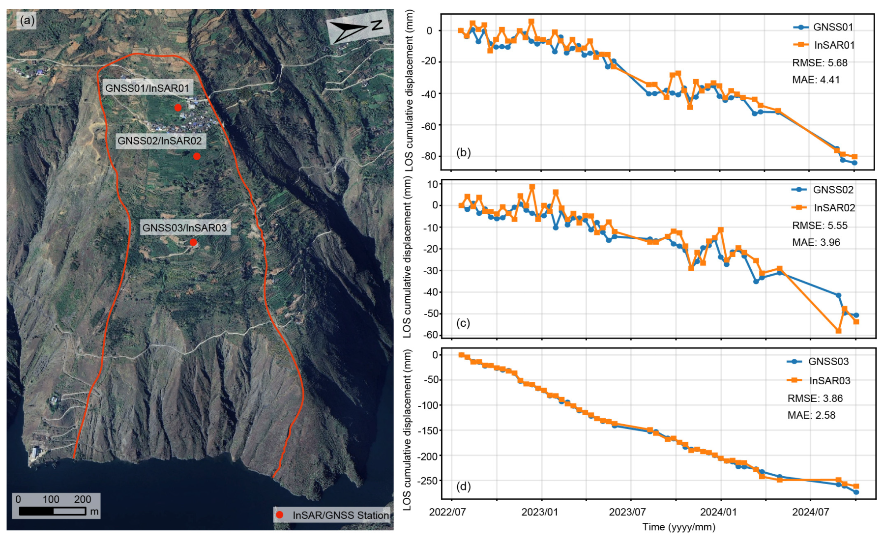
To evaluate the reliability of the 3D deformation inversion results, GNSS monitoring data from the Xiaomidi landslide in the Baihetan reservoir area were selected as independent validation data. Figure 8a shows the spatial distribution of the GNSS monitoring points and the corresponding InSAR measurement points at the Xiaomidi landslide. We selected the nearest valid InSAR measurement point within a 50 m search radius around each GNSS monitoring point, ensuring that the selected InSAR point was located within the same deformation zone. To ensure comparability between the two datasets, the east–west, north–south and vertical displacement components measured by GNSS were first projected onto the LOS direction according to the imaging geometries of the ascending and descending SAR tracks, and then resampled to the Sentinel-1 acquisition dates. Subsequently, the GNSS and InSAR time-series displacements were referenced to the same initial date, and the displacement at the initial epoch was set to zero, thereby eliminating the influence of differences in reference datum on the accuracy assessment. Because GNSS provides point-scale measurements, whereas InSAR represents the average displacement within a resolution cell, differences in observation scale, temporal sampling, and imperfect spatial collocation may contribute to local validation errors.

Figure 8b–d show the comparison results of the cumulative InSAR LOS displacement and the GNSS projected LOS displacement at the three monitoring points, respectively. Overall, the InSAR and GNSS time-series curves at the three monitoring points show good consistency in terms of variation trend and cumulative displacement amplitude, indicating that the InSAR LOS results can reliably reflect the continuous deformation process of the Xiaomidi landslide after impoundment. Among them, the LOS cumulative displacement at the GNSS01/InSAR01 points showed a gradually negative cumulative trend, with both types of data remaining consistent during the main deformation stage, and RMSE and MAE values of 5.68 mm and 4.41 mm, respectively. The GNSS02/InSAR02 points also exhibited continuous negative cumulative deformation characteristics. The InSAR results effectively captured the long-term trend of GNSS displacement, with RMSE and MAE values of 5.55 mm and 3.96 mm, respectively. The GNSS03/InSAR03 points had the largest cumulative displacement amplitude, indicating that this area was a region of strong deformation within the landslide. Meanwhile, the InSAR and GNSS curves at this point showed the best agreement, with RMSE and MAE values of 3.86 mm and 2.58 mm, respectively.

The LOS verification results show that the InSAR time-series displacements of the three monitoring points can well reflect the deformation trends observed by GNSS, and the errors are generally controlled within the millimeter to centimeter range, indicating that the LOS deformation results obtained by InSAR processing have high reliability. However, some differences still exist between the InSAR and GNSS curves in local time periods. This may be related to the different observation scales of the two technologies: GNSS reflects the 3D displacement of the monitoring pier location, while the InSAR measurement point represents the average LOS displacement within a certain spatial resolution pixel. Furthermore, atmospheric residual errors, coherence variations, temporal sampling differences, and the fact that the InSAR measurement points and GNSS points are not completely spatially aligned may also lead to slight deviations between the two types of results.

4.3.2. 3D Time-Series Displacement and Average Velocity Verification

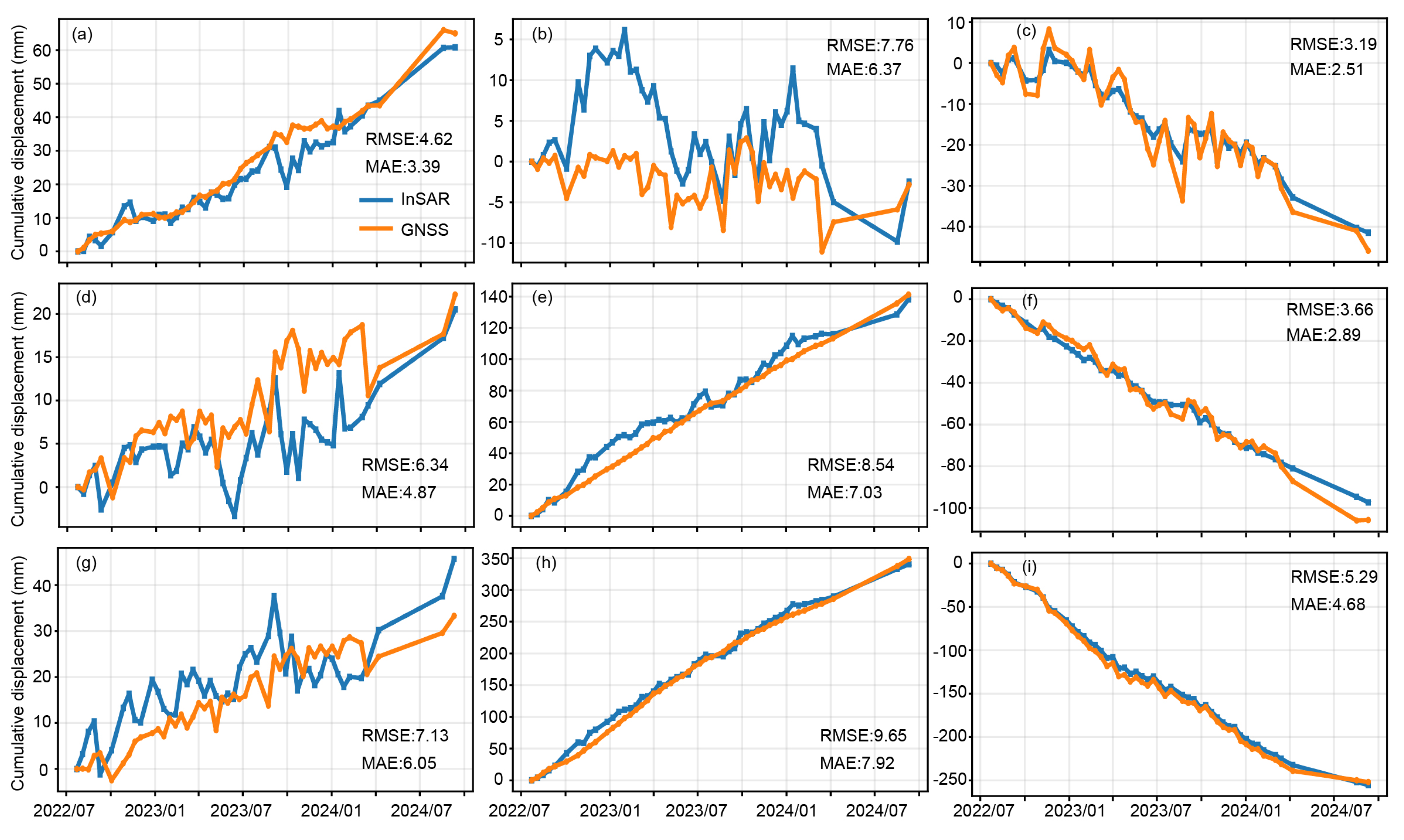
On the basis of validating the reliability of the LOS deformation results, we compared the 3D deformation components inverted by InSAR in the geodetic coordinate system with the GNSS displacement time series in the east–west, north–south and vertical directions. Figure 9 shows the component-wise validation results of the cumulative InSAR and GNSS displacements in the E, N and U directions at the three monitoring points.

For the GNSS01/InSAR01 point, the east–west and vertical components show good agreement, with RMSE/MAE values of 4.62/3.39 mm and 3.19/2.51 mm, respectively. For the GNSS02/InSAR02 point, the vertical component achieves high accuracy, with RMSE and MAE values of 3.66 mm and 2.89 mm, respectively. For the GNSS03/InSAR03 point, good consistency in temporal trend is maintained even under relatively large cumulative deformation, with vertical RMSE and MAE values of 5.29 mm and 4.68 mm, respectively. Overall, the vertical component shows the best validation performance, with RMSE values at the three monitoring points all below 5.29 mm and MAE values all below 4.68 mm. For the north–south component, which is more strongly affected by the limited geometric sensitivity of ascending and descending track LOS observations. Figure 9b,e,h show that the InSAR results can still reproduce the long-term displacement trends observed by GNSS. This indicates that the sensitivity-constrained regularization can enhance the inversion stability in weakly sensitive directions to some extent, thereby improving the overall reliability of the 3D deformation inversion results. The component-wise validation results show that the InSAR and GNSS time series curves at the three monitoring points are generally consistent in the east–west, north–south and vertical directions, demonstrating that the proposed method can effectively recover the 3D motion characteristics of the landslide.

Table 2. Comparison of 3D Deformation Velocity of GNSS and InSAR.

Monitoring Point Pair	Component	InSAR Velocity (mm/yr)	GNSS Velocity (mm/yr)	∆V (mm/yr)
GNSS01/InSAR01	E	25.59	28.47	2.88
	N	−4.13	−2.14	1.99
	U	−19.35	−20.86	1.52
GNSS02/InSAR02	E	5.97	9.52	3.55
	N	64.03	66.59	2.56
	U	−46.26	−48.70	2.44
GNSS03/InSAR03	E	13.15	16.87	3.73
	N	168.07	171.54	3.47
	U	−128.51	−129.40	0.88

shows the comparison results of the 3D average deformation velocities from GNSS and InSAR. The velocity differences in the E, N, and U directions at the three monitoring point pairs are all less than 4 mm/yr; the smallest difference is 0.88 mm/yr, occurring in the vertical component at the GNSS03/InSAR03 pair; the smallest difference in the north–south component is 1.99 mm/yr, occurring at the GNSS01/InSAR01 pair. The average value of the above nine sets of 3D velocity differences is approximately 2.56 mm/yr, indicating that the InSAR inversion results can not only reconstruct the 3D temporal displacement process well, but also accurately estimate the long-term average deformation velocity.

The validation results for the representative Xiaomidi landslide, including LOS time-series validation, 3D component-wise time-series validation and mean deformation velocity comparison, demonstrate that the proposed 3D deformation inversion method based on sensitivity-constrained regularization is reliable. Under dual-track InSAR observation conditions, the method can effectively recover 3D landslide motion information and can particularly characterize the vertical and dominant horizontal cumulative deformation features. For the weakly sensitive north–south component, the anisotropic regularization substantially improves the stability of the inversion.

5. Discussion

5.1. Evaluation of SC-Aniso Regularization Performance

5.1.1. Synthetic Validation of Recovery Accuracy in Weakly Sensitive Directions

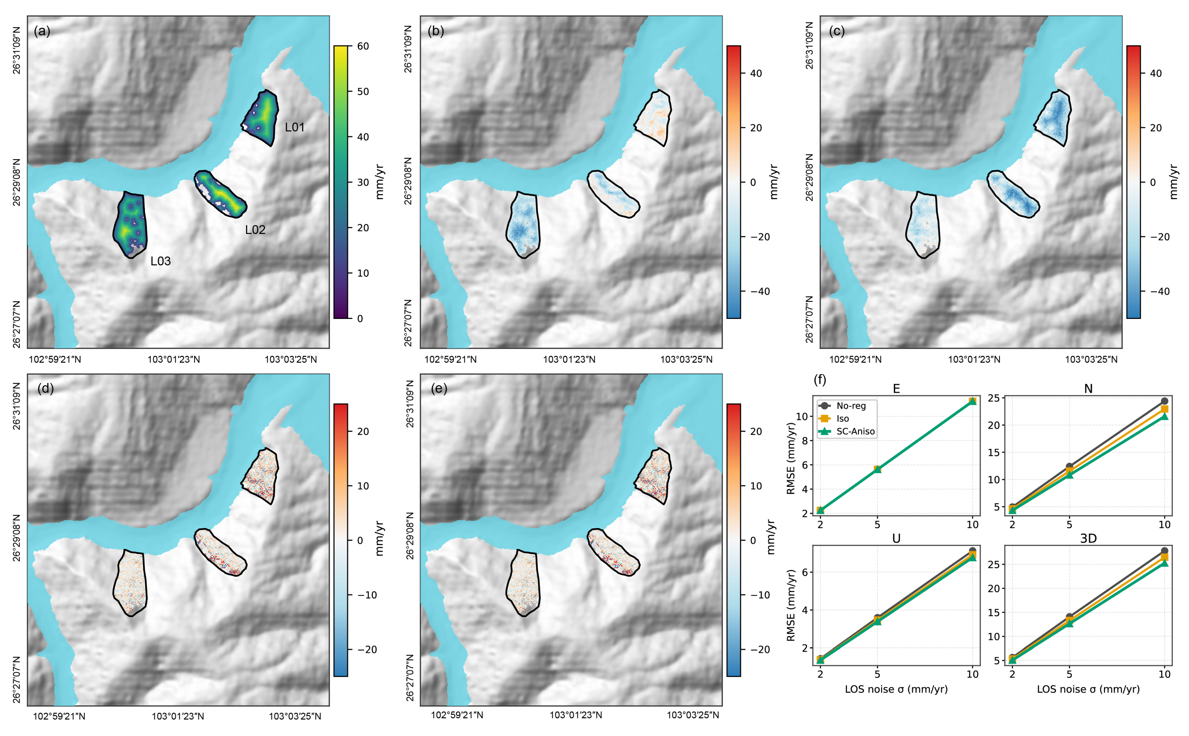
To verify whether our proposed SC-Aniso regularization method can improve the recovery accuracy of weakly sensitive directions, rather than simply reducing the discreteness of the inversion results, we conducted a synthetic experiment based on real terrain and Sentinel-1 ascending and descending track observation geometry. We selected three typical landslides, L01, L02, and L03, as shown in Figure 6. We selected landslides L01–L03 for testing the synthetic experiment. As described in Section 4.1, these areas were selected because they exhibit clear deformation signals in both ascending and descending track LOS results, and contain a sufficient number of common effective measurement points for two-track 3D inversion. We artificially constructed known slope direction velocity fields within the boundaries of the three landslides and converted them into a 3D ground truth field in geodetic coordinates using the local slope gradient of the DEM. We further projected this known 3D ground truth onto simulated ascending and descending track LOS observations using the ascending and descending track LOS unit vector, and superimposed Gaussian noise with standard deviations of 2, 5, and 10 mm/yr, respectively. We performed 3D inversion using three schemes: unregularized inversion, isotropic regularized, and SC-Aniso, and compared the inversion results with the known ground truth.

Figure 10 shows that the synthetic ascending and descending track LOS results exhibit clear differences in orbital geometry within the three landslides, indicating that the same 3D motion produces different projected responses along different LOS directions. Compared with isotropic regularization, SC-Aniso achieves lower north–south RMSE and overall 3D RMSE under all noise levels. Under LOS noise levels of 2–10 mm/yr, SC-Aniso reduces the north–south RMSE by approximately 5.91–6.27% and the overall 3D RMSE by approximately 4.58–4.87%. Although the magnitude of improvement is relatively modest, the improvement remains consistent across all three noise levels. This indicates that the enhancement of the weakly sensitive north–south component by SC-Aniso is stable, rather than being caused by a single noise level or by local anomalous pixels.

The purpose of this synthetic experiment is not to pursue a large reduction in RMSEs. Instead, under conditions of known ground truth and controlled noise, it aims to test whether SC-Aniso can provide a direction-selective stabilizing constraint for weakly sensitive directions. The consistent improvement observed under different noise levels indicates that the method enhances the robustness of dual-track 3D inversion, rather than simply compressing the numerical error. These results demonstrate that SC-Aniso not only suppresses unstable amplification in the north–south component, but also improves the recovery accuracy of both the weakly sensitive direction and the overall 3D deformation estimate under known ground truth conditions.

5.1.2. Effects of Different Regularization Strengths on 3D Deformation Stability

To evaluate the improvement effect of our proposed SC-Aniso method on the stability of 3D deformation inversion, we compared and analyzed the methods of unregularized inversion, traditional isotropic regularization, and the SC-Aniso method. Figure 11a shows that there are significant differences in the observation sensitivity of the ascending and descending track LOS geometry to different deformation components, with the north–south component showing the lowest sensitivity. This indicates that under direct solution or uniform constraint conditions, the north–south deformation is more susceptible to noise amplification and error propagation. The SC-Aniso method sets the direction regularization weights according to the inverse relationship of the observation geometry sensitivity, giving stronger constraints to the weakly sensitive north–south component, while imposing relatively weaker constraints on the vertical and east–west components. Therefore, our proposed method does not simply increase the overall regularization intensity, but rather utilizes the differences in SAR observation geometry to perform targeted stabilization processing on different directional components.

Figure 11b,c show the changes in 3D component stability and LOS fitting cost under different regularization intensities, respectively. As ${\lambda }_{reg}$ increases, the standard deviation of all directions within the stable LOS deformation region decreases overall, with the north–south component showing the most significant decrease, indicating that regularization effectively suppresses the amplification of instability in weakly sensitive directions. Compared with traditional isotropic regularization, the SC-Aniso method has a stronger stabilizing effect on the north–south component under the same regularization parameters, while the vertical and east–west components remain relatively stable. Meanwhile, Figure 11c shows that the all ascending and descending line-of-sight observations (All-LOS) RMSE gradually increases with ${\lambda }_{reg}$, which is a normal manifestation of the trade-off between observational fitting ability and solution stability in regularized inversion. Therefore, we did not use the minimum LOS RMSE or the minimum north–south standard deviation as the sole criterion, but instead considered both the LOS fitting cost and the stability of weakly sensitive directions.

To avoid subjective parameter selection, we applied the objective Pareto-knee criterion described in Section 3.2.3. For each candidate value, the All-LOS back-projection RMSE and the stable-area north–south standard deviation were log-transformed and independently normalized. We then selected the candidate with the maximum perpendicular distance to the chord connecting the two endpoints of the normalized curve. As shown in Figure 11d, this criterion yielded ${\mathsf{\lambda }}_{reg}$ = 0.015. At this value, the stability of the north–south component was substantially improved, while the All-LOS back-projection RMSE remained low.

Figure 11e compares the standard deviations of the three-dimensional components obtained using the unregularized inversion, isotropic regularization and SC-Aniso at ${\mathsf{\lambda }}_{reg}$. The results show that, under unregularized conditions, the standard deviation of the north–south component is significantly higher than those of the other components, indicating clear unstable amplification in the weakly sensitive direction. Although isotropic regularization reduces the overall dispersion, the north–south component remains relatively high. In contrast, the SC-Aniso method further reduces the north–south standard deviation without causing abnormal increases in the vertical or east–west components.

Figure 11f validates the stabilization effect of the SC-Aniso method on the north–south component from the perspective of discreteness indices. Compared with isotropic regularization, the SC-Aniso method not only reduces the ordinary standard deviation of the north–south direction, but also reduces the robust standard deviation based on the interquartile range and the 90% half-range, indicating that the method does not only weaken a few outliers, but also compresses the main range and tail dispersion of the north–south velocity distribution. Figure 11g summarizes the improvement of the SC-Aniso method compared with isotropic regularization and the corresponding LOS fitting cost. Around ${\mathsf{\lambda }}_{reg}$ = 0.015, the SC-Aniso method reduces the north–south standard deviation by about 41.9%, while the All-LOS RMSE only produces a small increment. This result shows that our proposed method can significantly improve the stability of the weakly sensitive north–south component with a small LOS fitting cost, thereby effectively improving the directional instability problem caused by observation geometric imbalance in dual-track InSAR 3D deformation inversion and improving the reliability of the 3D deformation solution.

5.2. 3D Deformation Characteristics and Field Evidence of Typical Landslide

The Xiaomidi landslide is located on the left-bank slope of the Jinsha River in the Baihetan reservoir area. The elevation of its rear scarp is approximately 1300–1360 m, and its front edge extends to the Jinsha River bank, with a relative elevation difference of approximately 710 m between the rear and front margins. The landslide is approximately 1100 m long in the longitudinal direction and 350–680 m wide in the transverse direction, with a projected area of approximately 55 × 104 m², indicating that it is a large reservoir-bank landslide. The upper and lower parts of the landslide are generally steep, whereas the middle part is relatively gentle.

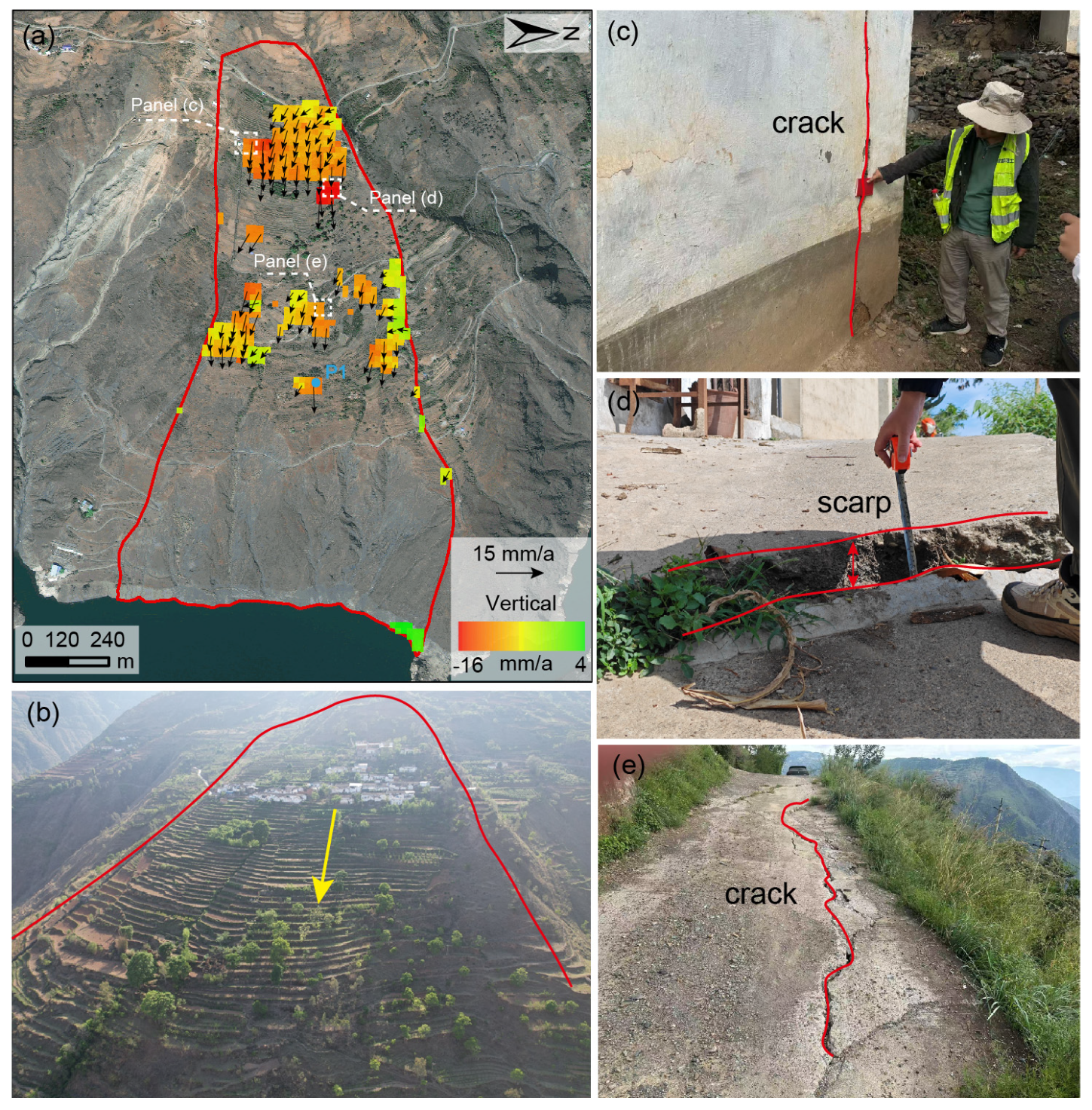
Figure 12a shows the 3D deformation inversion results of the Xiaomidi landslide, where colors represent vertical deformation rates, and black arrows represent horizontal deformation vectors synthesized from east–west and north–south deformation components. The results indicate that deformation within the landslide is not uniformly distributed but exhibits distinct regionalized concentrated activity characteristics. The vertical deformation is predominantly negative, with a maximum settlement rate of approximately −16 mm/yr, mainly concentrated in the upper and middle parts of the landslide and near the central terrace.

Figure 12a shows that the horizontal deformation vector of the landslide generally points towards the leading edge of the slope and the direction of the Jinsha River, which is largely consistent with the field-investigation result that the overall slope aspect of the landslide is approximately 95°. Locally, the upper and middle parts of the landslide are the main active area, with dense and long arrows indicating strong horizontal movement rates in this area. The vector of the active patch on the west side of the central part is slightly deflected to the southeast, while the active patch on the east side of the central part shows a certain eastward or east-northeast component, indicating the existence of differential movement and secondary deformation units within the landslide. The 3D deformation inversion relies on the common effective pixels from the ascending and descending track LOS observations. Due to differences in spatial coverage, coherence, and effective observation point distribution between the two-track data, the number of pixels satisfying the dual-track joint inversion conditions is relatively limited. Therefore, the spatial distribution of the 3D deformation results in Figure 12a is sparser than that of the single-track LOS results. However, these pixels are constrained by both ascending and descending track observations, and their inversion results can more robustly characterize the 3D movement direction and deformation intensity of the landslide.

Figure 12b shows that the main sliding direction identified in the field is generally consistent with the overall horizontal movement direction indicated by the 3D deformation vectors, suggesting that the inverted horizontal deformation vectors can effectively reflect the actual movement tendency of the landslide. The near-vertical cracks in building walls shown in Figure 12c, the surface scarps shown in Figure 12d, and the road cracks shown in Figure 12e all indicate ongoing tensile deformation, shearing and differential displacement within the landslide body. These field deformation features are mainly located within or near the active deformation zones identified in Figure 12a, further supporting the reliability of the 3D InSAR inversion results. Combining the vertical deformation velocity, horizontal deformation vectors and field deformation evidence, the Xiaomidi landslide is still in an active state. Its dominant deformation mode can be interpreted as a slow creeping process jointly controlled by settlement deformation in the middle–upper part and downslope movement towards the front edge.

5.3. Triggering Factors of the Typical Landslide

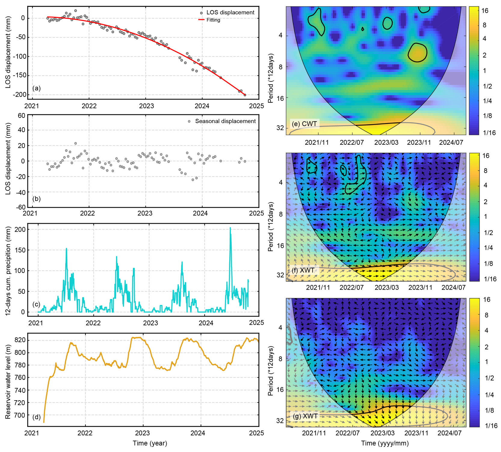
The motion of reservoir landslides is highly susceptible to precipitation and reservoir level fluctuations, because these factors can alter pore-water pressure within the slope and thereby affect slope stability [50,51,52]. To quantitatively investigate the relationship between the long-term displacement of the Xiaomidi landslide and precipitation and reservoir water level, we applied continuous wavelet transform (CWT) and cross-wavelet transform (XWT) techniques to identify periodic characteristics in the deformation time series. XWT was further used to reveal the common periodicity and time-lag effects between displacement and precipitation or reservoir water level. Specifically, we selected the LOS cumulative displacement series at point P1 in Figure 12a and combined it with 12-day cumulative precipitation and Baihetan reservoir water-level data for CWT and XWT analyses [53,54]. Daily precipitation data were obtained from the Climate Hazards Group InfraRed Precipitation with Station data (CHIRPS) [55], whereas daily reservoir-level data were derived from real-time water-level monitoring in the reservoir area.

To clarify the basis for calculating the lag times, we used phase difference analysis based on the XWT to determine the response lags of landslide displacement relative to precipitation and reservoir water level. The CWT was mainly used to identify the dominant period of the nonlinear displacement series. This procedure follows the continuous wavelet analysis and significance testing framework of Torrence and Compo [53], as well as the cross-wavelet and wavelet-coherence phase relationship analysis method of Grinsted et al. [54], and has been applied in analyses of InSAR landslide time series and their responses to hydrological factors [56]. Specifically, we first used a second-order polynomial to remove the long-term trend from the LOS cumulative displacement at point P1 and extracted the nonlinear seasonal displacement component. Daily precipitation data were then accumulated into a 12-day cumulative precipitation series consistent with the Sentinel-1 observation interval, and the reservoir water level series was resampled to the InSAR observation epochs. Lag estimation was performed only outside the cone of influence and within the 95% significant common power regions marked by the closed black contours. The phase arrows were used to indicate the leading or lagging relationship between two sets of sequences. The lag time was converted into actual time according to the proportion of the XWT phase difference within the significant common period band relative to the corresponding period. Since the sampling interval of the InSAR time series is 12 days, the temporal uncertainty of the lag estimates was considered to be on the order of one observation interval. The corresponding period was multiplied by 12 days during the conversion. Therefore, these values should be interpreted as approximate response times rather than exact daily scale values.

Figure 13a shows that the LOS displacement at point P1 exhibited a continuous negative cumulative trend from 2021 to 2024, indicating that the area at this point was in a state of continuous deformation after impoundment. After removing the long-term trend through second-order polynomial fitting, the nonlinear displacement component in Figure 13b showed significant seasonal fluctuations, indicating that the landslide deformation was controlled not only by long-term gravity creep but also by periodic external environmental factors. Figure 13c,d show that precipitation during the study period was mainly concentrated in the flood season, whereas the reservoir water level exhibited a distinct periodic rise-and-fall pattern. These two hydrological factors provide the basis for analysing the hydrological driving mechanism of landslide deformation.

The CWT result in Figure 13e shows that the detrended LOS displacement at point P1 has a strong energy distribution at approximately 24–32 Sentinel-1 observation cycles, corresponding to a time scale of about 288–384 days. This indicates that the deformation of the Xiaomidi landslide has significant seasonal to near-annual periodic characteristics. The periodic signal close to the annual scale is particularly prominent, suggesting that the nonlinear displacement of the landslide is mainly controlled by the annual hydrological cycle. XWT results show common high-energy regions between displacement and both precipitation and reservoir water level, indicating that both factors have potential driving effects on landslide deformation. In Figure 13f, the nonlinear displacement and 12-day cumulative precipitation exhibit a 95% significant common power region in the seasonal period band. Based on XWT phase difference analysis within this region, the average response lag of landslide deformation to precipitation is approximately 24 days, which is roughly equivalent to two Sentinel-1 observation intervals. Figure 13g shows that the nonlinear displacement and reservoir water level variations also exhibit a significant common power region in the longer seasonal to near-annual period band, but with a larger phase difference, corresponding to an average response lag of approximately 90 days. Because of the 12-day sampling interval of the InSAR time series, these two lag times should be interpreted as approximate response times rather than exact daily scale values. This time-lag effect suggests that precipitation and reservoir-level changes do not immediately enhance hillslope displacement; instead, their influence requires processes such as precipitation infiltration, groundwater recharge, pore-water pressure variation and internal stress redistribution within the hillslope.

Overall, Figure 13 indicates that the deformation process of the Xiaomidi landslide can be interpreted as a hydrologically controlled response under the background of long-term gravitational forcing, jointly regulated by precipitation infiltration and reservoir-level fluctuations. The response to precipitation is relatively rapid. Precipitation can infiltrate into the landslide body through cracks, loose deposits and fractured rock masses, increasing water content and pore-water pressure, reducing the shear strength of the sliding mass and promoting slow creep deformation. Periodic reservoir-level rise and fall alter the seepage field and hydraulic boundary conditions near the slope toe, and affect landslide stability through groundwater recharge and internal pore-pressure adjustment. In particular, during rapid reservoir-level fluctuations, pore-water pressure adjustment within the hillslope often lags behind external water-level changes, resulting in a longer time-lag effect of reservoir-level variation on landslide deformation [51,52,57].

5.4. Methodological Discussion

3D InSAR deformation monitoring generally requires three independent observation components with substantially different viewing geometries [10,11,12]. However, in studies of landslides in mountainous areas, the available observations are often limited to ascending and descending track LOS measurements because of Sentinel-1 orbital coverage, coherence loss and topographic shadowing. The surface-parallel flow assumption provides an important physical constraint for 3D inversion under dual-track conditions [14,15,16,19,20,21,58]. Its central premise is that landslide motion is primarily gravity-driven and occurs approximately along the local slope surface. It should be emphasized that pixel-scale or local-gradient surface-parallel flow concepts have already been explored in previous studies [15,16,19,20,58]. In this study, the local surface-parallel flow constraint is used as a topographic prior, rather than being presented as a completely independent new theory beyond existing SPFM or pixel-wise SPFM approaches. On this basis, the core methodological contribution of this study is SC-Aniso, which explicitly incorporates the directional sensitivity of ascending and descending track LOS observations into the design of regularization weights, thereby constraining the instability of weakly sensitive directions under dual-track viewing geometry.

Although LGSPFM serves as a supporting topographic prior in this study, its implementation depends on local gradients derived from the smoothed DEM. We tested eight Gaussian smoothing scales, with σ values ranging from 0.1 to 5.0 pixels and kernel sizes ranging from 3 × 3 to 41 × 41 pixels. This analysis evaluated whether changes in the smoothing scale propagated into the final 3D inversion. As shown in

Table 3. Sensitivity of the LGSPFM-constrained 3D inversion to Gaussian DEM smoothing parameters.

Gaussian Standard Deviation, σ (pixel)	Kernel Size (pixel)	DEM Smoothing Deviation RMSE (m)	Gradient Roughness, Rpq	All-LOS Back-Projection RMSE (mm/yr)
0.1	3 × 3	0.000	0.239	0.734
0.5	5 × 5	1.798	0.181	0.751
1.0	9 × 9	4.965	0.098	0.791
1.5	13 × 13	6.569	0.068	0.806
2.0	17 × 17	8.058	0.052	0.810
3.0	25 × 25	11.176	0.035	0.813
4.0	33 × 33	14.477	0.027	0.807
5.0	41 × 41	17.888	0.022	0.796

, local-gradient roughness gradually decreased as σ increased, whereas the modification of the original DEM increased. When σ increased from 0.1 to 1.0 pixels, R_pq decreased from 0.239 to 0.098, representing a reduction of approximately 58.8%. At this scale, the DEM smoothing deviation RMSE was 4.965 m. Further increases in σ continued to reduce gradient roughness but caused greater modification of the DEM. They did not produce a consistent improvement in the All-LOS back-projection RMSE. We therefore adopted σ = 1.0 pixel and the corresponding 9 × 9-pixel kernel as a conservative compromise between suppressing pixel-scale gradient fluctuations and preserving local terrain variations. Across all tested scales, the All-LOS back-projection RMSE ranged from 0.734 to 0.813 mm/yr. This range indicates that the overall fit of the 3D inversion remained relatively stable.

In addition to the topographic constraint, dual-track InSAR 3D inversion is affected by directional imbalance in the observation geometry. Ascending and descending track Sentinel-1 LOS observations are much less sensitive to the north–south component than to the east–west and vertical components [10,11,12,22,23]. Therefore, direct inversion or isotropic regularization may amplify noise in the weakly observed direction. This may hinder the stable interpretation of 3D motion vectors. SC-Aniso addresses this problem within a generalized anisotropic Tikhonov framework. It maps the inverse joint root-mean-square sensitivities of the actual two-track observation geometry to the relative penalty weights for the E, N, and U components. These weights are neither empirically prescribed nor independently tuned. Only one global regularization parameter needs to be selected during the inversion. The main innovation is that LOS sensitivity is converted from a diagnostic measure of observational capability into an active model-space constraint. This constraint is further coupled with LGSPFM. In this framework, SAR viewing geometry determines the numerical stabilization strength for each deformation component. Meanwhile, pixel-scale DEM geometry provides a physically meaningful surface-parallel motion prior. The proposed method therefore better represents the inherent imbalance in the sensitivity of SAR observation geometry to different 3D deformation components. Figure 10 and Figure 11 show that this design selectively stabilizes the weakly observed north–south component. It also improves the recovery accuracy of this component while causing only a small increase in the LOS back-projection error.

Despite these improvements, the physical reliability of the recovered north–south component requires careful qualification. It is jointly inferred from ascending and descending track LOS observations and the LGSPFM prior. Therefore, it should be regarded as a model-constrained estimate rather than an independent direct observation. SC-Aniso improves the numerical stability of this component. However, it does not increase the intrinsic sensitivity of the dual-track observation geometry to north–south motion or eliminate the geometric blind spot. Stronger damping suppresses noise amplification and reduces solution variance. It may also attenuate some local deformation amplitudes because of regularization-induced shrinkage. In the synthetic experiments, the north–south RMSE decreased by 5.91–6.27% relative to isotropic regularization. In the real-data analysis, the stable-area north–south standard deviation decreased by 41.9%. The north–south rate differences at the three GNSS sites ranged from 1.99 to 3.47 mm/yr. These results support the physical interpretation of the deformation sign, coherent spatial pattern, long-term trend, and mean rate of the recovered north–south component. However, isolated pixels, short-term fluctuations, local extrema, and exact local amplitudes should still be interpreted with caution.

The advantages of the proposed method are also reflected in the interpretation of the results. By transforming the 3D deformation components from the geodetic coordinate system into the slope coordinate system, the downslope, normal-to-slope and cross-slope components can be used to characterize hillslope movement, local compression or settlement, and lateral shearing, respectively. This provides a more intuitive kinematic basis for identifying landslide activity zones and deformation patterns. The GNSS validation, field evidence of cracks and surface scarps, and rainfall–reservoir-level time–frequency analysis of the Xiaomidi landslide jointly demonstrate that the dual-track inversion framework, centered on SC-Aniso and combined with local surface constraints, can not only recover the 3D landslide deformation field but also support mechanistic interpretation of representative landslides. Compared with previous InSAR based landslide studies that mainly focused on LOS monitoring [4,5,59,60,61,62,63,64,65], 2D identification [17,18] and time series interpretation [56,57,61,62,66], the proposed framework further strengthens the connection between landslide 3D motion decomposition and observation-sensitivity constraints, thereby improving the physical consistency and stability of the inversion.

In this study, another limitation arises from the phase-based LOS inputs. They have incomplete spatial coverage and limited data quality. In the E-SBAS processing, we integrated DS and PS observations and set a 60-day temporal baseline threshold to improve measurement point coverage, but decorrelation could not be completely eliminated in areas with dense vegetation, steep terrain, or rapid local deformation [40]. Therefore, phase-based InSAR results preferentially reflect the relatively coherent parts of the landslide body, and the deformation range or local maximum deformation of the landslide may be underestimated in areas of low coherence or failed phase unwrapping. This limitation is even more pronounced in 3D results because 3D inversion can only use pixels that are valid for both ascending and descending tracks. Therefore, the lack of valid measurement points cannot be interpreted as the absence of deformation. We did not employ amplitude or pixel offset tracking (POT) primarily because landslides in the study area are mainly characterized by slow deformation, and the displacement between adjacent Sentinel-1 images is much smaller than the image resolution. POT generally has lower measurement accuracy than phase-based InSAR. It is more suitable for large or rapid deformations with clear and temporally stable intensity characteristics [67].

6. Conclusions

This study addresses the core challenge of stably recovering three-dimensional deformation of complex reservoir-bank landslides under dual-track InSAR conditions. We developed a 3D deformation inversion framework centered on SC-Aniso and incorporating LGSPFM as a topographic prior. Using 340 ascending and descending Sentinel-1A images, we derived post-impoundment LOS time-series deformation and 3D deformation velocity fields for the Baihetan Reservoir area during 2021–2024. The results show weak background deformation across the reservoir area, with anomalies mainly concentrated on local steep slopes along both banks of the Jinsha River and in representative reservoir-bank landslide zones. The inverted 3D fields reveal compound motion in landslides L01–L03, including subsidence, horizontal displacement, and downslope creep.

The primary methodological contribution of this study is SC-Aniso, which adaptively assigns directional regularization weights according to the sensitivity of ascending and descending LOS track observations to vertical, east–west, and north–south deformation components. This strategy mitigates the instability of the weakly sensitive north–south component, while the LGSPFM constraint helps represent complex and non-uniform local slope geometry in deep canyon reservoir areas. Synthetic experiments show that SC-Aniso reduces the north–south RMSE by 5.91–6.27% and the overall 3D RMSE by 4.58–4.87% compared with isotropic regularization. At the objectively selected parameter, ${\mathsf{\lambda }}_{reg}$ = 0.015, the north–south standard deviation decreases by 41.9%, with only a slight increase in LOS fitting cost. GNSS validation shows vertical RMSEs below 5.29 mm and average E, N, and U rate differences below 4 mm/yr. These results demonstrate that the proposed method can reliably recover 3D landslide motion under limited two-track observations.

The Xiaomidi landslide remained active after impoundment, showing slow creep controlled by middle–upper subsidence, horizontal displacement, and downslope movement toward the front edge. CWT and XWT analyses reveal a 288–384-day seasonal period in nonlinear displacement, with lags of approximately 24 and 90 days relative to rainfall and reservoir water-level variation, respectively. This indicates that the landslide is a hydrologically responsive reservoir-bank landslide regulated by rainfall infiltration and reservoir-level fluctuations under long-term gravitational creep.

In summary, the proposed dual-track 3D InSAR inversion framework centered on SC-Aniso can provide technical support for stable recovery of 3D deformation, reliable estimation of weakly sensitive directions, interpretation of movement mechanisms and post-impoundment risk diagnosis of complex reservoir-bank landslides.

References

1. Yin, Y.; Huang, B.; Wang, W.; Wei, Y.; Ma, X.; Ma, F.; Zhao, C. Reservoir-induced landslides and risk control in Three Gorges Project on Yangtze River, China. J. Rock. Mech. Geotech. Eng. 2016, 8, 577–595. [Google Scholar] [CrossRef]
2. Wang, F.; Zhang, Y.; Huo, Z.; Peng, X.; Araiba, K.; Wang, G. Movement of the Shuping landslide in the first four years after the initial impoundment of the Three Gorges Dam Reservoir, China. Landslides 2008, 5, 321–329. [Google Scholar] [CrossRef]
3. Huang, X.; Guo, F.; Deng, M.; Yi, W.; Huang, H. Understanding the deformation mechanism and threshold reservoir level of the floating weight-reducing landslide in the Three Gorges Reservoir Area, China. Landslides 2020, 17, 2879–2894. [Google Scholar] [CrossRef]
4. Hilley, G.E.; Buergmann, R.; Ferretti, A.; Novali, F.; Rocca, F. Dynamics of slow-moving landslides from permanent scatterer analysis. Science 2004, 304, 1952–1955. [Google Scholar] [CrossRef] [PubMed]
5. Cascini, L.; Fornaro, G.; Peduto, D. Analysis at medium scale of low-resolution DInSAR data in slow-moving landslide-affected areas. ISPRS J. Photogramm. Remote Sens. 2009, 64, 598–611. [Google Scholar] [CrossRef]
6. Ferretti, A.; Prati, C.; Rocca, F. Permanent scatterers in SAR interferometry. IEEE Trans. Geosci. Remote Sens. 2001, 39, 8–20. [Google Scholar] [CrossRef]
7. Berardino, P.; Fornaro, G.; Lanari, R.; Sansosti, E. A new algorithm for surface deformation monitoring based on small baseline differential SAR interferograms. IEEE Trans. Geosci. Remote Sens. 2002, 40, 2375–2383. [Google Scholar] [CrossRef]
8. Rosen, P.A.; Hensley, S.; Joughin, I.R.; Li, F.K.; Madsen, S.N.; Rodriguez, E.; Goldstein, R.M. Synthetic aperture radar interferometry. Proc. IEEE 2000, 88, 333–382. [Google Scholar] [CrossRef]
9. Massonnet, D.; Feigl, K.L. Radar interferometry and its application to changes in the Earth’s surface. Rev. Geophys. 1998, 36, 441–500. [Google Scholar] [CrossRef]
10. Hu, J.; Li, Z.W.; Ding, X.L.; Zhu, J.J.; Zhang, L.; Sun, Q. Resolving three-dimensional surface displacements from InSAR measurements: A review. Earth Sci. Rev. 2014, 133, 1–17. [Google Scholar] [CrossRef]
11. Wright, T.J.; Parsons, B.E.; Lu, Z. Toward mapping surface deformation in three dimensions using InSAR. Geophys. Res. Lett. 2004, 31, L01607. [Google Scholar] [CrossRef]
12. Fuhrmann, T.; Garthwaite, M.C. Resolving Three-Dimensional Surface Motion with InSAR: Constraints from Multi-Geometry Data Fusion. Remote Sens. 2019, 11, 241. [Google Scholar] [CrossRef]
13. Samsonov, S.; D’Oreye, N. Multidimensional time-series analysis of ground deformation from multiple InSAR data sets applied to Virunga Volcanic Province. Geophys. J. Int. 2012, 191, 1095–1108. [Google Scholar] [CrossRef]
14. Joughin, I.R.; Kwok, R.; Fahnestock, M.A. Interferometric estimation of three-dimensional ice-flow using ascending and descending passes. IEEE Trans. Geosci. Remote Sens. 1998, 36, 25–37. [Google Scholar] [CrossRef]
15. Ao, M.; Zhang, L.; Shi, X.; Liao, M.; Dong, J. Measurement of the three-dimensional surface deformation of the Jiaju landslide using a surface-parallel flow model. Remote Sens. Lett. 2019, 10, 776–785. [Google Scholar] [CrossRef]
16. Liu, X.; Zhao, C.; Zhang, Q.; Yin, Y.; Lu, Z.; Samsonov, S.; Yang, C.; Wang, M.; Tomas, R. Three-dimensional and long-term landslide displacement estimation by fusing C- and L-band SAR observations: A case study in Gongjue County, Tibet, China. Remote Sens. Environ. 2021, 267, 112745. [Google Scholar] [CrossRef]
17. Eriksen, H.Ø.; Lauknes, T.R.; Larsen, Y.; Corner, G.D.; Bergh, S.G.; Dehls, J.; Kierulf, H.P. Visualizing and interpreting surface displacement patterns on unstable slopes using multi-geometry satellite SAR interferometry (2D InSAR). Remote Sens. Environ. 2017, 191, 297–312. [Google Scholar] [CrossRef]
18. Meng, Q.; Confuorto, P.; Peng, Y.; Raspini, F.; Bianchini, S.; Han, S.; Liu, H.; Casagli, N. Regional Recognition and Classification of Active Loess Landslides Using Two-Dimensional Deformation Derived from Sentinel-1 Interferometric Radar Data. Remote Sens. 2020, 12, 1541. [Google Scholar] [CrossRef]
19. Liu, D.; Zeng, B.; Xu, H.; Yuan, J. Three-dimensional deformation monitoring of landslides based on combination of two-track InSAR observations and pixel-level surface-parallel flow model. Int. J. Remote Sens. 2024, 45, 8380–8404. [Google Scholar] [CrossRef]
20. Zheng, W.; Hu, J.; Lu, Z.; Hu, X.; Sun, Q.; Liu, J.; Zhu, J.; Li, Z. Enhanced Kinematic Inversion of 3-D Displacements, Geometry, and Hydraulic Properties of a North-South Slow-Moving Landslide in Three Gorges Reservoir. J. Geophys. Res. Solid Earth 2023, 128, e2022JB026232. [Google Scholar] [CrossRef]
21. Ren, K.; Yao, X.; Li, R.; Zhou, Z.; Yao, C.; Jiang, S. 3D displacement and deformation mechanism of deep-seated gravitational slope deformation revealed by InSAR: A case study in Wudongde Reservoir, Jinsha River. Landslides 2022, 19, 2159–2175. [Google Scholar] [CrossRef]
22. Dai, K.; Deng, J.; Xu, Q.; Li, Z.; Shi, X.; Hancock, C.; Wen, N.; Zhang, L.; Zhuo, G. Interpretation and sensitivity analysis of the InSAR line of sight displacements in landslide measurements. GISci. Remote Sens. 2022, 59, 1226–1242. [Google Scholar] [CrossRef]
23. Van Natijne, A.L.; Bogaard, T.A.; van Leijen, F.J.; Hanssen, R.F.; Lindenbergh, R.C. World-wide InSAR sensitivity index for landslide deformation tracking. Int. J. Appl. Earth Obs. Geoinf. 2022, 111, 102829. [Google Scholar] [CrossRef]
24. Tikhonov, A.N.; Arsenin, V.Y. Solutions of Ill-Posed Problems; Winston: Washington, DC, USA; Wiley: New York, NY, USA, 1977. [Google Scholar]
25. Li, L.; Xu, C.; Yao, X.; Shao, B.; Ouyang, J.; Zhang, Z.; Huang, Y. Large-scale landslides around the reservoir area of Baihetan Hydropower Station in Southwest China: Analysis of the spatial distribution. Nat. Hazards Res. 2022, 2, 218–229. [Google Scholar] [CrossRef]
26. Zhang, R.; Zhao, X.; Dong, X.; Dai, K.; Deng, J.; Zhuo, G.; Yu, B.; Wu, T.; Xiang, J. Potential Landslide Identification in Baihetan Reservoir Area Based on C-/L-Band Synthetic Aperture Radar Data and Applicability Analysis. Remote Sens. 2024, 16, 1591. [Google Scholar] [CrossRef]
27. Yao, J.; Wang, T.; Yao, X. Spatial-temporal evolution of landslides spanning the impoundment of Baihetan mega hydropower project revealed by satellite radar interferometry. Remote Sens. Environ. 2025, 321, 114668. [Google Scholar] [CrossRef]
28. Yao, C.; Li, L.; Yao, X.; Li, R.; Ren, K.; Jiang, S.; Chen, X.; Ma, L. Study on the Identification, Failure Mode, and Spatial Distribution of Bank Collapses after the Initial Impoundment in the Head Section of Baihetan Reservoir in Jinsha River, China. Remote Sens. 2024, 16, 2253. [Google Scholar] [CrossRef]
29. Fu, G.; She, Y.; Zhang, G.; Wang, Y.; Gao, S.; Liu, T. Lithospheric Equilibrium, Environmental Changes, and Potential Induced-Earthquake Risk around the Newly Impounded Baihetan Reservoir, China. Remote Sens. 2021, 13, 3895. [Google Scholar] [CrossRef]
30. Zhou, Z.K.; Yao, X.; Li, R.J.; Jiang, S.; Zhao, X.M.; Ren, K.Y.; Zhu, Y.F. Deformation characteristics and mechanism of an impoundment-induced toppling landslide in Baihetan Reservoir based on multi-source remote sensing. J. Mt. Sci. 2023, 20, 3614–3630. [Google Scholar] [CrossRef]
31. Yi, X.; Feng, W.; Wu, M.; Ye, Z.; Fang, Y.; Wang, P.; Li, R.; Dun, J. The initial impoundment of the Baihetan Reservoir region (China) exacerbated the deformation of the Wangjiashan landslide: Characteristics and mechanism. Landslides 2022, 19, 1897–1912. [Google Scholar] [CrossRef]
32. Torres, R.; Snoeij, P.; Geudtner, D.; Bibby, D.; Davidson, M.; Attema, E.; Potin, P.; Rommen, B.; Floury, N.; Brown, M.; et al. GMES Sentinel-1 mission. Remote Sens. Environ. 2012, 120, 9–24. [Google Scholar] [CrossRef]
33. Reyes-Carmona, C.; Barra, A.; Galve, J.P.; Monserrat, O.; Perez-Pena, J.V.; Mateos, R.M.; Notti, D.; Ruano, P.; Millares, A.; Lopez-Vinielles, J.; et al. Sentinel-1 DInSAR for Monitoring Active Landslides in Critical Infrastructures: The Case of the Rules Reservoir (Southern Spain). Remote Sens. 2020, 12, 809. [Google Scholar] [CrossRef]
34. Alaska Satellite Facility. ALOS PALSAR High Resolution Radiometric Terrain Corrected Product; NASA Alaska Satellite Facility Distributed Active Archive Center: Fairbanks, AK, USA, 2015. [Google Scholar] [CrossRef]
35. Yu, C.; Li, Z.; Penna, N.T.; Crippa, P. Generic Atmospheric Correction Model for Interferometric Synthetic Aperture Radar Observations. J. Geophys. Res. Solid Earth 2018, 123, 9202–9222. [Google Scholar] [CrossRef]
36. Cigna, F.; Tapete, D. Sentinel-1 Big Data Processing with P-SBAS InSAR in the Geohazards Exploitation Platform: An Experiment on Coastal Land Subsidence and Landslides in Italy. Remote Sens. 2021, 13, 885. [Google Scholar] [CrossRef]
37. Hooper, A.; Zebker, H.; Segall, P.; Kampes, B. A new method for measuring deformation on volcanoes and other natural terrains using InSAR persistent scatterers. Geophys. Res. Lett. 2004, 31, L23611. [Google Scholar] [CrossRef]
38. Lanari, R.; Mora, O.; Manunta, M.; Mallorqui, J.J.; Berardino, P.; Sansosti, E. A small-baseline approach for investigating deformations on full-resolution differential SAR interferograms. IEEE Trans. Geosci. Remote Sens. 2004, 42, 1377–1386. [Google Scholar] [CrossRef]
39. Ferretti, A.; Fumagalli, A.; Novali, F.; Prati, C.; Rocca, F.; Rucci, A. A new algorithm for processing interferometric data-stacks: SqueeSAR. IEEE Trans. Geosci. Remote Sens. 2011, 49, 3460–3470. [Google Scholar] [CrossRef]
40. Zebker, H.A.; Villasenor, J. Decorrelation in interferometric radar echoes. IEEE Trans. Geosci. Remote Sens. 1992, 30, 950–959. [Google Scholar] [CrossRef]
41. Goldstein, R.M.; Werner, C.L. Radar interferogram filtering for geophysical applications. Geophys. Res. Lett. 1998, 25, 4035–4038. [Google Scholar] [CrossRef]
42. Hanssen, R.F. Radar Interferometry: Data Interpretation and Error Analysis; Kluwer Academic Publishers: Dordrecht, The Netherlands, 2001. [Google Scholar] [CrossRef]
43. Hansen, P.C. Analysis of discrete ill-posed problems by means of the L-curve. SIAM Rev. 1992, 34, 561–580. [Google Scholar] [CrossRef] [PubMed]
44. Mehrabi, H.; Voosoghi, B.; Motagh, M.; Hanssen, R.F. Three-Dimensional Displacement Fields from InSAR through Tikhonov Regularization and Least-Squares Variance Component Estimation. J. Surv. Eng. 2019, 145, 04019011. [Google Scholar] [CrossRef]
45. Wang, Z.; Liu, G.; Hu, L.; Tao, Q.; Yu, S. Method for Determining Weight Matrix for Resolving Three-Dimensional Surface Deformation Using Multi-LOS D-InSAR Technology. Int. J. Appl. Earth Obs. Geoinf. 2020, 88, 102062. [Google Scholar] [CrossRef]
46. Gholami, A.; Gazzola, S. Robust Estimation of Structural Orientation Parameters and 2D/3D Local Anisotropic Tikhonov Regularization. Geophysics 2024, 89, V521–V536. [Google Scholar] [CrossRef]
47. Calvetti, D.; Somersalo, E. Distributed Tikhonov Regularization for Ill-Posed Inverse Problems from a Bayesian Perspective. Comput. Optim. Appl. 2025, 91, 541–572. [Google Scholar] [CrossRef]
48. Schier, P.; Liebl, M.; Steinhoff, U.; Handler, M.; Wiekhorst, F.; Baumgarten, D. Optimizing Excitation Coil Currents for Advanced Magnetorelaxometry Imaging. J. Math. Imaging Vis. 2020, 62, 238–252. [Google Scholar] [CrossRef]
49. Das, I. On Characterizing the “Knee” of the Pareto Curve Based on Normal-Boundary Intersection. Struct. Optim. 1999, 18, 107–115. [Google Scholar] [CrossRef]
50. Zhao, S.; Zeng, R.; Zhang, H.; Meng, X.; Zhang, Z.; Meng, X.; Wang, H.; Zhang, Y.; Liu, J. Impact of Water Level Fluctuations on Landslide Deformation at Longyangxia Reservoir, Qinghai Province, China. Remote Sens. 2022, 14, 212. [Google Scholar] [CrossRef]
51. Yang, Z.; Li, Z.; Zhu, J.; Yi, H.; Hu, J.; Feng, G. Time-lag response of landslide to reservoir water level variation during the impoundment of the Baihetan Reservoir area. Water 2023, 15, 2732. [Google Scholar] [CrossRef]
52. Huang, F.; Huang, J.; Jiang, S.; Zhou, C. Stability analysis of hydrodynamic pressure landslides with different permeability coefficients affected by reservoir water level fluctuations and rainstorms. Water 2017, 9, 450. [Google Scholar] [CrossRef]
53. Torrence, C.; Compo, G.P. A practical guide to wavelet analysis. Bull. Am. Meteorol. Soc. 1998, 79, 61–78. [Google Scholar] [CrossRef]
54. Grinsted, A.; Moore, J.C.; Jevrejeva, S. Application of the cross wavelet transform and wavelet coherence to geophysical time series. Nonlinear Processes Geophys. 2004, 11, 561–566. [Google Scholar] [CrossRef]
55. Funk, C.; Peterson, P.; Landsfeld, M.; Pedreros, D.; Verdin, J.; Shukla, S.; Husak, G.; Rowland, J.; Harrison, L.; Hoell, A.; et al. The climate hazards infrared precipitation with stations-a new environmental record for monitoring extremes. Sci. Data 2015, 2, 150066. [Google Scholar] [CrossRef] [PubMed]
56. Tomás, R.; Li, Z.; Lopez-Sanchez, J.M.; Liu, P.; Singleton, A. Using wavelet tools to analyse seasonal variations from InSAR time-series data: A case study of the Huangtupo landslide. Landslides 2016, 13, 437–450. [Google Scholar] [CrossRef]
57. Shi, X.; Hu, X.; Buergmann, R.; Yu, C.; Lu, Z.; Liu, J.; Qu, F. Hydrological control shift from river level to rainfall in the reactivated Guobu slope beside the Laxiwa hydropower station, China. Remote Sens. Environ. 2021, 265, 112664. [Google Scholar] [CrossRef]
58. Jia, H.; Wang, Y.; Ge, D.; Deng, Y.; Wang, R. InSAR Study of Landslides: Early Detection, Three-Dimensional, and Long-Term Surface Displacement Estimation-A Case of Xiaojiang River Basin, China. Remote Sens. 2022, 14, 1759. [Google Scholar] [CrossRef]
59. Herrera, G.; Gutierrez, F.; Garcia-Davalillo, J.C.; Guerrero, J.; Notti, D.; Galve, J.P.; Cooksley, G. Multi-sensor advanced DInSAR monitoring of very slow landslides: The Tena Valley case study (central Spanish Pyrenees). Remote Sens. Environ. 2013, 128, 31–43. [Google Scholar] [CrossRef]
60. Frattini, P.; Crosta, G.B.; Rossini, M.; Allievi, J. Activity and kinematic behaviour of deep-seated landslides from PS-InSAR displacement rate measurements. Landslides 2018, 15, 1053–1070. [Google Scholar] [CrossRef]
61. Xie, M.; Zhao, W.; Ju, N.; He, C.; Huang, H.; Cui, Q. Landslide evolution assessment based on InSAR and real-time monitoring of a large reactivated landslide, Wenchuan, China. Eng. Geol. 2020, 277, 105781. [Google Scholar] [CrossRef]
62. Dong, J.; Zhang, L.; Tang, M.; Liao, M.; Xu, Q.; Gong, J.; Ao, M. Mapping landslide surface displacements with time series SAR interferometry by combining persistent and distributed scatterers: A case study of Jiaju landslide in Danba, China. Remote Sens. Environ. 2018, 205, 180–198. [Google Scholar] [CrossRef]
63. Colesanti, C.; Wasowski, J. Investigating landslides with space-borne Synthetic Aperture Radar (SAR) interferometry. Eng. Geol. 2006, 88, 173–199. [Google Scholar] [CrossRef]
64. Wasowski, J.; Bovenga, F. Investigating landslides and unstable slopes with satellite Multi Temporal Interferometry: Current issues and future perspectives. Eng. Geol. 2014, 174, 103–138. [Google Scholar] [CrossRef]
65. Bekaert, D.P.S.; Handwerger, A.L.; Agram, P.; Kirschbaum, D.B. InSAR-based detection method for mapping and monitoring slow-moving landslides in remote regions with steep and mountainous terrain: An application to Nepal. Remote Sens. Environ. 2020, 249, 111983. [Google Scholar] [CrossRef]
66. Kang, Y.; Lu, Z.; Zhao, C.; Xu, Y.; Kim, J.-W.; Gallegos, A.J. InSAR monitoring of creeping landslides in mountainous regions: A case study in Eldorado National Forest, California. Remote Sens. Environ. 2021, 258, 112400. [Google Scholar] [CrossRef]
67. Shi, X.; Zhang, L.; Balz, T.; Liao, M. Landslide Deformation Monitoring Using Point-Like Target Offset Tracking with Multi-Mode High-Resolution TerraSAR-X Data. ISPRS J. Photogramm. Remote Sens. 2015, 105, 128–140. [Google Scholar] [CrossRef]
Figure 1. Panels showing: (a) Geographical location of the study area. (b) Stratigraphic lithology of the study area. (c) Overall view of the Baihetan Dam site. (d) Wulipo landslide. (e) Changdi landslide. (f) Xiaomidi landslide.
Remotesensing 18 02525 g001
Figure 2. Flowchart of the proposed sensitivity-constrained 3D deformation inversion method.
Remotesensing 18 02525 g002
Figure 3. Sentinel-1A SAR data coverage over the study area (ascending track: Path 26, Frames 78 and 83; descending track: Path 62, Frames 504 and 499).
Remotesensing 18 02525 g003
Figure 4. Schematic diagram of 3D deformation projection and slope-coordinate transformation based on two-track InSAR observations and LGSPFM constraints: (a) LOS projection of 3D deformation in the geodetic coordinate frame with pixel-scale DEM-derived elevation gradients. (b) Transformation of 3D deformation components into the slope coordinate frame.
Remotesensing 18 02525 g004
Figure 5. Relationship between sensitivity index and directional regularization parameter.
Remotesensing 18 02525 g005
Figure 6. LOS deformation velocity after impoundment. (a) Ascending track LOS deformation velocity; (b) enlarged view of the ascending track LOS deformation velocity in the selected landslide areas; (c) descending track LOS deformation velocity; (d) enlarged view of the descending-track LOS deformation velocity in the selected landslide areas; (e) frequency distribution of ascending track LOS deformation velocities; (f) frequency distribution of descending track LOS deformation velocities.
Remotesensing 18 02525 g006
Figure 7. Post-impoundment 3D deformation velocity fields in the geodetic and local slope coordinates. Panels (a,b), (c,d), and (e,f) show the vertical, north–south, and east–west components, respectively; the first panel in each pair is regional, and the second enlarges landslides L01–L03. Panels (g,h), (i,j), and (k,l) show the downslope, normal-to-slope, and cross-slope components, respectively. Positive geodetic values indicate upward, northward, and eastward motion, respectively. Negative slope-coordinate values indicate downslope motion, motion toward the slope surface, and right-lateral cross-slope motion, respectively.
Remotesensing 18 02525 g007
Figure 8. Comparison of InSAR LOS time-series deformation and GNSS monitoring accuracy for the Xiaomidi landslide. (a) Distribution map of landslide monitoring points. (b) Time-series comparison of GNSS01 and InSAR01. (c) Time-series comparison of GNSS02 and InSAR02. (d) Time-series comparison of GNSS03 and InSAR03.
Remotesensing 18 02525 g008
Figure 9. Validation of time-series comparisons of 3D deformation components between GNSS and InSAR. (ac) Time-series verification of GNSS01 and InSAR01 in the E, N, and U directions, respectively. (df) Time-series verification of GNSS02 and InSAR02 in the E, N, and U directions, respectively. (gi) Time-series verification of GNSS03 and InSAR03 in the E, N, and U directions, respectively.
Remotesensing 18 02525 g009
Figure 10. Synthetic validation of SC-Aniso regularization based on representative landslide boundaries. (ac) Prescribed downslope velocity and synthetic ascending/descending LOS velocities; (d,e) north–south component errors under isotropic and SC-Aniso regularization; (f) mean RMSE under different LOS noise levels.
Remotesensing 18 02525 g010
Figure 11. Panels showing: (a) LOS geometric sensitivity and directional regularization weights; (b,c) 3D-component standard deviations in stable LOS areas and All-LOS back-projection RMSE under different regularization strengths; (d) stability–fitting Pareto curve displayed in the original physical units, with the optimal SC-Aniso parameter selected using the maximum-distance criterion in normalized log–log space; (e) component standard deviations under different methods at the selected regularization parameter; (f,g) north–south dispersion metrics and stability improvement relative to isotropic regularization.
Remotesensing 18 02525 g011
Figure 12. Panels showing: (a) 3D deformation inversion results and deformation vector distribution of the Xiaomidi landslide; (b) overall geomorphic view of the representative landslide and its main sliding direction; (c) tensile cracking in building walls; (d) surface scarp deformation; (e) development of road cracks.
Remotesensing 18 02525 g012
Figure 13. Time frequency response and lag relationship between deformation of the Xiaomidi landslide and precipitation–reservoir water level driving factors. (a) LOS cumulative displacement and fitted trend; (b) detrended seasonal LOS displacement; (c) 12-day cumulative precipitation; (d) reservoir water level; (e) CWT of the InSAR deformation series; (f,g) XWT between InSAR deformation and precipitation/reservoir water level. The black contours indicate regions significant at the 95% confidence level, and the curved boundary denotes the cone of influence. The phase arrows indicate the relative phase relationship.
Remotesensing 18 02525 g013